This document discusses Python and its use for scientific computing and solar physics. It provides a brief introduction to Python and key scientific Python packages like NumPy, Matplotlib, and SciPy. It then discusses how Python is used for tasks in solar physics, including reading solar data files and working with spatially aware maps. The document encourages the use of Python and participation in the SunPy community.

1. Steven Christe1,, Matt Earnshaw2, Keith Hughitt1, Jack Ireland1, Florian Mayer3,
Albert Shih1, Alex Young1
1 NASA GSFC
2 Imperial College London
3 Vienna University of Technology
Florian Mayer

2.  What is Python?
 Introduction to Python
 Scientific Python
 NumPy
 Matplotlib
 SciPy
 Python in solar physics

3.  General-purpose
 Object-oriented (disputed)
 Cross-platform
 Windows
 Mac OS
 Linux
 Other Unices (FreeBSD, Solaris, etc.)
 High-level

4.  Internet companies
 Google
 Rackspace
 Games
 Battlefield 2
 Civilization 4
 Graphics
 Walt Disney
 Science
 NASA
 ESRI

5.  Easy
 Comprehensive standard library (“batteries
included”)
Quality does vary, though.
 Good support for scientific tasks
 Permissive open-source license
On the downside:
 Slower, but ways to speed up

6. PYTHON IDL
 Free open-source software  Proprietary software
 Without cost  License cost
 General purpose  Small community
 Good plotting  Cumbersome plotting
 No solar software  Solar software

7.  Implementation started 1989 by Guido van
Rossum (BDFL)
 2.0 appeared 2000
 Garbage collection
 Unicode
 3.0 appeared 2008

8.  Astronomy
 Artificial intelligence & machine learning
 Bayesian Statistics
 Biology (including Neuroscience)
 Dynamical systems
 Economics and Econometrics
 Electromagnetics
 Electrical Engineering
 Geosciences
 Molecular modeling
 Signal processing
 Symbolic math, number theory

9.  pyFITS – read FITS files
 pyRAF – run IRAF tasks
 pywcs
 pyephem – compute positions of objects in
space
 spacepy (space sciences, just released)
 Planned standard library AstroPy

10.  Beautiful is better than ugly.
 Explicit is better than implicit.
 Simple is better than complex.
 Readability counts.
 There should be one – and preferably only
one – obvious way to do it.
 Although that way may not be obvious at first
unless you're Dutch.
 >>> import this

11. Brief introduction into Python

12.  Infix notation operations
 Python 2 defaults to floor division
 More mathematical operations in math
 Complex math in cmath

13.  Integers are arbitrary size.
 Floats are platform doubles.
 decimal module for arbitrary precision
decimal numbers
 fractions module for fractions

14. STRINGS / BYTES UNICODE
 "foo"  u"foo"
 Store bytes  Store unicode codepoints
 Useful for binary data  Useful for text
 Behave as expected for
multibyte characters

15.  [1, 2, 3, 4]  (1, u"foo")
 Mutable  Immutable
 Multiple records  Different objects
describing one record

16.  if/elif/else
 for-loop
 break
 continue
 else
 while-loop
 pass

17.  Default arguments are evaluated once at
compile time!
 lambda alternative syntax for definition of
trivial functions
 Functions are objects, too!

18.  Unordered key-value mappings
 Approx. O(1) lookup and storage
 Keys must be immutable (hashable)

19.  Unordered collection of unique objects
 Approx. O(1) membership test
 Members must be immutable (hashable)

20.  Classes
 Explicit self
 Multiple inheritance
 Also in IDL 8; no escaping it

21.  try / except / else
 raise
 Exceptions inherit from Exception

22. PYTHON 2.7 PYTHON 3.2
 Print statement  Print function
 String / Unicode  Bytes / String
 Floor division  Float Division
 Relative imports  Absolute imports
 Lists  Views
Tons of other changes
http://bit.ly/newpy3

23.  Fundamental package for science in Python
 Multidimensional fixed-size, homogenous
arrays
 Derived objects: e.g. matrices
 More efficient
 Less code

24.  Python list
 arange
 linspace / logspace
 ones / zeros / eye / diag
 random

25.  Absence of explicit looping
 Conciseness – less bugs
 Closer to mathematical notation
 More pythonic.
 Also possible for user functions

26.  Expansion of multidimensional arrays
 Implicit element-by-element behavior

33.  Boolean area
 Integer area

34. Type Remarks Character code
byte compatible: C char 'b'
short compatible: C short 'h'
intc compatible: C int 'i'
int_ compatible: Python int 'l'
longlong compatible: C long long 'q'
large enough to fit a
intp 'p'
pointer
int8 8 bits
int16 16 bits
int32 32 bits
int64 64 bits

35. Type Remarks Character code
ubyte compatible: C u. char 'B'
ushort compatible: C u. short 'H'
uintc compatible: C unsigned int 'I'
uint compatible: Python int 'L'
ulonglong compatible: C long long 'Q'
large enough to fit a
uintp 'P'
pointer
uint8 8 bits
uint16 16 bits
uint32 32 bits
uint64 64 bits

36. Type Remarks Character code
half 'e'
single compatible: C float 'f'
double compatible: C double
float_ compatible: Python float 'd'
longfloat compatible: C long float 'g'
float16 16 bits
float32 32 bits
float64 64 bits
float96 96 bits, platform?
float128 128 bits, platform?

37. Type Remarks Character code
csingle 'F'
compatible: Python
complex_ 'D'
complex
clongfloat 'G'
complex64 two 32-bit floats
complex128 two 64-bit floats
two 96-bit floats,
complex192
platform?
two 128-bit floats,
complex256
platform?

38.  NumPy: weave.blitz (fast NumPy
expressions)
 NumPy: weave.inline (inline C/C++)
 f2py (interface Fortran)
 Pyrex/Cython (python-like compiled
language)

39.  2D plotting library
 Some 3D support
 Publication-quality
figures
 “Make easy things easy
and hard things
possible”
 Configurable using
matplotlibrc

40. import numpy as np
from matplotlib import pyplot as plt
t = np.linspace(0, 2, 200)
s = np.sin(2*pi*t)
plt.plot(t, s, linewidth=1.0)
plt.xlabel('time (s)')
plt.ylabel('voltage (mV)')
plt.title('About as simple as it gets, folks')
plt.grid(True)
plt.show()

41. import numpy as np
from matplotlib import pyplot as plt
def f(t):
s1 = np.cos(2*pi*t)
e1 = np.exp(-t)
return np.multiply(s1,e1)
t1 = np.arange(0.0, 5.0, 0.1)
t2 = np.arange(0.0, 5.0, 0.02)
t3 = np.arange(0.0, 2.0, 0.01)
plt.subplot(211)
l = plot(t1, f(t1), 'bo', t2, f(t2), 'k--',
markerfacecolor='green')
plt.grid(True)
plt.title('A tale of 2 subplots')
plt.ylabel('Damped oscillation')
plt.subplot(212)
plt.plot(t3, np.cos(2*pi*t3), 'r.')
plt.grid(True)
plt.xlabel('time (s)')
plt.ylabel('Undamped')
plt.show()

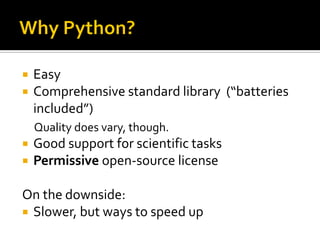
42. import numpy as np
import matplotlib.path as mpath
import matplotlib.patches as mpatches
import matplotlib.pyplot as plt
Path = mpath.Path
fig = plt.figure()
ax = fig.add_subplot(111)
pathdata = [
(Path.MOVETO, (1.58, -2.57)),
(Path.CURVE4, (0.35, -1.1)),
(Path.CURVE4, (-1.75, 2.0)),
(Path.CURVE4, (0.375, 2.0)),
(Path.LINETO, (0.85, 1.15)),
(Path.CURVE4, (2.2, 3.2)),
(Path.CURVE4, (3, 0.05)),
(Path.CURVE4, (2.0, -0.5)),
(Path.CLOSEPOLY, (1.58, -2.57)),
]
codes, verts = zip(*pathdata)
path = mpath.Path(verts, codes)
patch = mpatches.PathPatch(path, facecolor='red',
edgecolor='yellow', alpha=0.5)
ax.add_patch(patch)
x, y = zip(*path.vertices)
line, = ax.plot(x, y, 'go-')
ax.grid()
ax.set_xlim(-3,4)
ax.set_ylim(-3,4)
ax.set_title('spline paths')
plt.show()

43. from mpl_toolkits.mplot3d import Axes3D
from matplotlib import cm
from matplotlib.ticker import (LinearLocator, FixedLocator,
FormatStrFormatter)
import matplotlib.pyplot as plt
import numpy as np
fig = plt.figure()
ax = fig.gca(projection='3d')
X = np.arange(-5, 5, 0.25)
Y = np.arange(-5, 5, 0.25)
X, Y = np.meshgrid(X, Y)
R = np.sqrt(X**2 + Y**2)
Z = np.sin(R)
surf = ax.plot_surface(X, Y, Z, rstride=1, cstride=1,
cmap=cm.jet,
linewidth=0, antialiased=False)
ax.set_zlim3d(-1.01, 1.01)
ax.w_zaxis.set_major_locator(LinearLocator(10))
ax.w_zaxis.set_major_formatter(FormatStrFormatter('%.03f'))
fig.colorbar(surf, shrink=0.5, aspect=5)
plt.show()

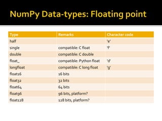
44. import numpy as np
from matplotlib import pyplot as plt
from matplotlib.patches import Ellipse
NUM = 250
ells = [
Ellipse(xy=rand(2)*10, width=np.rand(),
height=np.rand(), angle=np.rand()*360)
for i in xrange(NUM)]
fig = plt.figure()
ax = fig.add_subplot(111, aspect='equal')
for e in ells:
ax.add_artist(e)
e.set_clip_box(ax.bbox)
e.set_alpha(rand())
e.set_facecolor(rand(3))
ax.set_xlim(0, 10)
ax.set_ylim(0, 10)
plt.show()

47.  Statistics
 Optimization
 Numerical integration
 Linear algebra
 Fourier transforms
 Signal processing
 Image processing
 ODE solvers
 Special functions
 And more.

48.  Three phases
 Glass sample – light grey
 Bubbles – black
 Sand grains – dark grey
 Determine
 Fraction of the sample
covered by these
 Typical size of sand
grains or bubbles

49. 1. Open image and examine it
2. Crop away panel at bottom
 Examine histogram
3. Apply median filter
4. Determine thresholds
5. Display colored image
6. Use mathematical morphology to clean the
different phases
7. Attribute labels to all bubbles and sand grains
 Remove from the sand mask grains that are smaller
than 10 pixels
8. Compute the mean size of bubbles.

50.  Spatially aware maps
 Read FITS files
 RHESSI
 SDO/AIA
 EIT
 TRACE
 LASCO
 standard color tables and hist equalization
 basic image coalignment
 VSO
 HEK

51.  Spatially aware array
 NumPy array
 Based on SolarSoft Map.
 MapCube

52.  Two APIs
 Legacy API (tries to mimic IDL vso_search)
 New API based on boolean operations

53.  Create VSO queries from HER responses
 WIP: Plot HER events over images

55.  Use it!
 File feature requests
 Express opinion on the mailing list / in IRC
 File bug reports
 Contribute documentation
 Contribute code

56.  Website: http://sunpy.org
 Mailing list: http://bit.ly/sunpy-forum
 IRC: #sunpy on irc.freenode.net
 Git code repository:
https://github.com/sunpy/sunpy

57.  Email: florian.mayer@bitsrc.org
 IRC: __name__ in #sunpy on freenode
 XMPP: segfaulthunter@jabber.ccc.de

58.  SciPy: http://scipy.org
 Astronomical modules: http://bit.ly/astropy
 Science modules: http://bit.ly/sciencepy
 NumPy/IDL: http://hvrd.me/numpy-idl
 Python for interactive data analysis:
http://bit.ly/pydatatut
 SciPy lecture notes: http://bit.ly/scipylec
 This talk: http://graz-talk.bitsrc.org
 SunPy doc: http://sunpy.org/doc/

59.  Steven Christe1,
 Matt Earnshaw2
 Keith Hughitt1
 Jack Ireland1 Thanks to
 Florian Mayer3
 Albert Shih1
 Alex Young1
1 NASA GSFC
2 Imperial College London
3 Vienna University of Technology