Programming And Scientific Computing In Python 60 Jm Hoekstra
Programming And Scientific Computing In Python 60 Jm Hoekstra
Programming And Scientific Computing In Python 60 Jm Hoekstra
Programming And Scientific Computing In Python 60 Jm Hoekstra
Programming And Scientific Computing In Python 60 Jm Hoekstra
1.
Programming And ScientificComputing In Python
60 Jm Hoekstra download
https://ebookbell.com/product/programming-and-scientific-
computing-in-python-60-jm-hoekstra-51055746
Explore and download more ebooks at ebookbell.com
2.
Here are somerecommended products that we believe you will be
interested in. You can click the link to download.
Ocaml Scientific Computing Functional Programming In Data Science And
Artificial Intelligence Liang Wang
https://ebookbell.com/product/ocaml-scientific-computing-functional-
programming-in-data-science-and-artificial-intelligence-liang-
wang-43400394
Matlab And Simulink In Action Programming Scientific Computing And
Simulation Dingy Xue
https://ebookbell.com/product/matlab-and-simulink-in-action-
programming-scientific-computing-and-simulation-dingy-xue-57087372
Python Programming Versatile Highlevel Language For Rapid Development
And Scientific Computing Mastering Programming Languages Series Edet
https://ebookbell.com/product/python-programming-versatile-highlevel-
language-for-rapid-development-and-scientific-computing-mastering-
programming-languages-series-edet-71592228
Principles Of Parallel Scientific Computing A First Guide To Numerical
Concepts And Programming Methods Tobias Weinzierl
https://ebookbell.com/product/principles-of-parallel-scientific-
computing-a-first-guide-to-numerical-concepts-and-programming-methods-
tobias-weinzierl-38376354
3.
Scientific Programming NumericSymbolic And Graphical Computing With
Maxima 1st Edition Jorge Alberto Calvo
https://ebookbell.com/product/scientific-programming-numeric-symbolic-
and-graphical-computing-with-maxima-1st-edition-jorge-alberto-
calvo-34588190
Introduction To Scientific Programming And Simulation Using R 1st
Edition Owen Jones
https://ebookbell.com/product/introduction-to-scientific-programming-
and-simulation-using-r-1st-edition-owen-jones-55441006
Introduction To Scientific Programming And Simulation Using R 2nd
Edition Owen Jones
https://ebookbell.com/product/introduction-to-scientific-programming-
and-simulation-using-r-2nd-edition-owen-jones-5066656
Introduction To Modern Scientific Programming And Numerical Methods
Lubos Brieda Joseph Wang Robert Martin
https://ebookbell.com/product/introduction-to-modern-scientific-
programming-and-numerical-methods-lubos-brieda-joseph-wang-robert-
martin-59715628
Classical Fortran Programming For Engineering And Scientific
Applications 2nd Edition Kupferschmid
https://ebookbell.com/product/classical-fortran-programming-for-
engineering-and-scientific-applications-2nd-edition-
kupferschmid-5066472
Preface
The first versionof this reader was developed for, and during the pilot of, the Programming course in
the first year of the BSc program Aerospace Engineering at the Delft University of Technology in 2012.
Originally it was written for Python 2 and then converted to Python 3.
The goal of the Python programming course is to enable the student to:
• write a program for scientific computing
• develop models
• analyse behaviour of the models, for instance using plots
• visualise models by animating graphics
The course assumes some mathematical skills, but no programming experience whatsoever.
This document is provided as a reference for the elaboration of the assignments. The reader is en-
couraged to read through the relevant chapters applicable to a particular problem. For later reference,
many tables, as well as some appendices with quick reference guides, have been included. These
encompass the most often used functions and methods. For a complete overview, there is the excel-
lent documentation as provided with Python in the IDLE Help menu, as well as the downloadable and
on-line documentation for the Python modules NumPy, SciPy, Matplotlib and Pygame.
Also, the set-up of the present course is to show the appeal of programming. Having this powerful tool
at hand allows the reader to use the computer as a ‘mathematical slave’. And by making models, one
basically has the universe in a sandbox at one’s disposal: Any complex problem can be programmed
and displayed, from molecular behaviour to the motion in a complex gravity field in space.
An important ingredient at the beginning of the course is the ability to solve mathematical puzzles and
numerical problems. Also the very easy to use graphics module Pygame module has been included in
this reader. This allows, next to the simulation of a physical problem, a real-time visualization and some
control (mouse and keyboard) for the user, which also adds some fun for the beginning and struggling
programmer in the form of visual feedback.
Next to the mathematical puzzles, challenges (like Project Euler and the Python challenge) and simu-
lations and games, there is a programming contest included in the last module of the course for which
there is a prize for the winners. Often students surprise me with their skills and creativity in such a
contest by submitting impressive simulations and games.
Also check out the accompanying videos: Search for “AE1205” on Youtube.
Many thanks to the students and teaching assistants, whose questions, input and feedback formed the
foundation for this reader.
J.M. Hoekstra and J. Ellerbroek
Delft, March 2022
iii
9.
Reading guide
This readeris intended to be used as reference material during the course, as well as during the exams.
To guide you through the reader, the following is useful to know:
Throughout the reader, most material counts as exam material. Some parts, however, are optional.
You can recognise optional parts as follows:
• Within chapters, small optional parts (that for instance dive deeper into a concept, or provide an
alternative approach) are encapsulated in blue boxes that are marked extra:
Extra: The explanation in this box isn’t exam material
Very deep contemplations go here!
• When an entire chapter is optional, its chapter number will be marked with a red asterisk: ∗
.
Coloured boxes are also used to mark or reiterate something that is important:
NB: An important remark
Make sure not to skip these boxes!
In each chapter, several sections have exercises related to the presented material. The answers to
these numbered exercises can be found in several places:
• In Appendix A.
• As Python files on https://github.com/TUDelft-AE-Python/ae1205-exercises/ in
the folder pyfiles.
• As Jupyter notebooks on https://github.com/TUDelft-AE-Python/ae1205-exercises/
in the folder notebooks.
The exam of the Python course is an open-book exam: you are allowed to use an original bound copy
of the reader during the entire exam. Sometimes it’s useful to read something back in detail in one of
the chapters, but often just a quick reminder will be enough. In the latter case you can use the course
cheat sheet in Appendix C.
v
1
Getting started
1.1. Whatis programming?
Ask a random individual what programming is and you will get a variety of answers. Some love it. Some
hate it. Some call it mathematics, others philosophy, and making models in Python is mostly a part of
physics. More interestingly, many different opinions exist on how a program should be written. Many
experienced programmers tend to believe they see the right solution in a flash, while others say it always
has to follow a strict phased design process, starting with thoroughly analysing the requirements (the
‘bookkeeper’ style). It definitely is a skill and personally I think a well written, easy to read and effective
piece of code with a brilliant algorithm, is also a piece of art. Programming does not require a lot of
knowledge, it is a way of thinking and it becomes an intuition after a lot of experience.
This also means that learning to program is very different from the learning you do in most other courses.
In the beginning, there is a very steep learning curve, but once you have taken the first big step, it will
become much easier and a lot of fun. But how and when you take that first hurdle is very personal.
Of course, you first need to achieve the right rate of success over failure, something you can achieve
by testing small parts during the development. For me, there aren’t many things that give me more
pleasure than to see my program (finally) work. The instant, often visual, feedback makes it a very
rewarding activity.
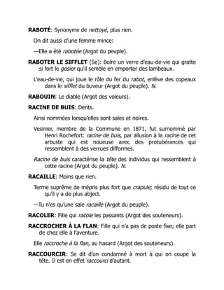
start
Switch on heating
?
Get desired
temperature
Measure room
temperature
Switch off heating
True
False
Figure 1.1: Flow chart of ‘thermostat’ algorithm
And even though at some stage you will also see
the right solution method in a flash, at the same time
your program will almost certainly not work the first
time you run it. A lot of time is spent understanding
why it will not work and fixing this. Therefore some
people call the art of programming: “solving puzzles
created by your own stupidity”!
While solving these puzzles, you will learn about
logic, you will learn to think about thinking.
The first step towards a program is always to decom-
pose a problem into smaller steps, into ever smaller
building blocks to describe the so-called algorithm.
An algorithm is a list of actions and decisions that a
computer (or a person) has to go through chronolog-
ically to solve a problem.
This is often schematically presented in the form of
a flow chart. For instance, the algorithm of a ther-
mostat that has to control the room temperature is
shown in Figure 1.1.
1
16.
2 1. Gettingstarted
Another way to design and represent algorithms is using simplified natural language. Let’s take as an
example the algorithm to “find the maximum value of four numbers”. We can detail this algorithm as a
number of steps:
Algorithm: Find the maximum of four numbers
Let's call the 4 numbers a, b, c and d
if a > b then make x equal to a, else make x equal to b
if c < d then make y equal to c, else make y equal to d
if x < y then make x equal to y
show result x on screen
Going through these steps, the result will always be that the maximum value of the four numbers is
shown on the screen. This kind of description in natural language is called “pseudo-code”.
This pseudo-code is already very close to how Python looks, as this was one the goals of Python:
it should read just as clear as pseudo-code. But before we can look at some real Python code, we
need to know what Python is and how you can install it. After that, we will have a look at some simple
programs in Python, which you can try out in your freshly installed Python environment.
1.2. What is Python?
Python is a general purpose programming language. And even though until a few years ago Python
was used more in the USA than in Europe, it has been developed by a Dutchman, Guido van Rossum.
It all started as a hobby project, which he pursued in his spare time while still employed at the so-called
Centrum Wiskunde & Informatica (CWI) in Amsterdam in 1990. Python was named after Monty Python
and references to Monty Python in comments and examples are still appreciated. The goals of Python,
as Guido van Rossum has formulated them in a 1999 DARPA proposal, are:
• an easy and intuitive language just as powerful as major competitors
• open source, so anyone can contribute to its development
• code that is as understandable as plain English
• suitable for everyday tasks, allowing for short development times
Guido van Rossum was employed by Google for many years, as this is one of the many companies
that use Python. He briefly retired in 2019, only to return back from retirement to join the Development
Division at Microsoft. As moderator of the Python language he used to be called the “benevolent dictator
for life” until he stepped down from the position in July 2018.
A practical advantage of Python is that it supports many platforms (Windows, Apple, Linux) and that it
is free, and so are all add-ons. Many add-ons have been developed by the large (academic) Python
community. Some have become standards of their own, such as the scientific package NumPy/SciPy/-
Matplotlib. These scientific libraries (or modules as they are called in Python), in syntax(grammar)
heavily inspired by the software package MATLAB, are now the standard libraries for scientific com-
puting in Python. IEEE has named Python as the de facto standard programming language for data
analysis.
Up to Python 3 all versions were downwards compatible. So all past programs and libraries will still
work in a newer Python 2.x versions. However, at some point, Guido van Rossum, being the BDFL
(Benevolent Dictator For Life) of Python, wanted to correct some fundamental issues, which could only
be done by breaking the downward compatibility. This started the development of Python 3.0. For a
long time Python 2.x was also still maintained and updated. This has stopped around 2018.
An example of a difference between the two versions is the syntax of the print-function, which shows
a text or a number on the screen during runtime of the program:
17.
1.3. Installing Python3
Python 2 vs. Python 3
# Python 2.x:
print ”Hello world”
# Python 3.x:
print(”Hello World”)
(Other major differences relate to integer division and the input() function. You will learn more about
these concepts during the course).
Python is called a scripting language. This means that the Python source is interpreted when you run
the program as opposed to needing to compile all program files first, then link them together with the
correct libraries to make an executable and then run this. This is very user-friendly: there is no need to
compile or link files before you can run the same program on any operating system: Windows, Apple’s
macOS or Linux. While many Python libraries are platform dependent, most are available on all three
supported platforms.
The penalty for this is, depending on your program structure, sometimes some execution speed. Some
runtime, often seconds or milliseconds, are traded for shorter development times, which saves time in
the order of days or weeks. Note that Python libraries like NumPy and Scipy use very fast low-level
modules, resulting in extremely fast execution times for scientific computing. By using a similar syntax,
this is replacing MATLAB (which also uses a small scripting language) worldwide. Using vectorised
programming and the NumPy library makes runtimes comparable with optimised C++ and Fortran for
the scientific computing. The same mechanism allows fast graphics. For example for 2D graphics the
Pygame graphics library, which is a layer over the very fast and famous SDL library, is also extremely
fast.
Using an interpreter instead of a compiler, means you need to have Python, with its interpreter, installed
on the computer where you run the Python program. Would you ever want to make an executable to
avoid this requirement, there are modules, like distutils, or add-ons, like called Py2exe creating self-
contained application which does not need Python installed. Such an executable will only run on the
OS under which it was compiled. How this should be done, is covered by a separate chapter of the
reader, called ‘Distributing your Python program’. Using the Inno Setup tool, you can make a installer
for your application on Windows for example. This tool converts the complete folder with data and the
program into one setup executable file, which is also covered in this chapter.
1.3. Installing Python
For each platform there are several ways to install Python. In this reader we’ll give instructions for Win-
dows, macOS, and Linux for which we’ve found that they result in the least number of problems.
1.3.1. Windows
In Windows there are three main ways to install Python; starting out with a plain package from the official
distributor, using a bundle like Anaconda, and installing python through the Microsoft Store.
We’ve found that the most robust way to install Python is by starting out with a plain installation of
Python, from the official python website. Go to Python.org and download the latest version of Python 3
64-bits. (You can also check out the steps at Youtube: https://youtu.be/-P7dVLJPows)
If you’re installing Python a second time, then make sure you have uninstalled/removed any other
versions of Python, using the Add/Remove Apps/Programs from the Settings/Configuration panel of
Windows.
Once you’ve downloaded the installer, run it, and:
18.
4 1. Gettingstarted
1. During the installation, when you get the dialog indicated below, make sure you tick the box ‘Add
Python 3.X to PATH’! (otherwise the Python package installer pip will not work)
2. Choose ‘Customize installation’
3. In the dialog that follows, check all options, especially ‘install for all users’
4. Click ‘Install’ to start a full installation of Python
When the installation finishes you’ll not only have Python, but also the Python package manager pip
installed, which makes it relatively simple to install the other packages. Pip makes sure to download
the exactly right version for your installation of Python and OS and will install it.
The next step is to install the Python packages you’ll need during the course. In the Windows Start
Menu, search for command prompt:
Right-click on the result, and click ‘Run as Administrator’.
In the command window that has opened, type
pip3 install numpy scipy matplotlib pygame
19.
1.3. Installing Python5
1.3.2. macOS
By default, macOS already has Python installed, on recent macOS versions even Python 3.8. However,
these preinstalled versions have some issues, specifically with the installation of packages needed for
the course. It is therefore required to install an additional version of Python on your Mac. The currently
recommended method for this is to use the official Python installer from python.org:
1. In your browser, navigate to python.org, and in the ‘Downloads’ menu, click on the download
link of the current Python version for macOS.
2. Once downloaded, open the installer, which will give you the following dialog:
Follow the dialog steps. Unless you want a different installation location (not recommended),
there’s no need to make any changes to the default settings.
3. Once the installation is finished, a finder window is opened, showing the results of the Python
installation.
4. To install the packages required for this course, you need to open a terminal. Simultaneously
press the ‘command’ and space keys, type the word terminal, and press enter:
5. In the terminal that has opened, type
pip3 install numpy scipy matplotlib pygame A dialog will open, requesting you to
provide your user password (required to execute a command as Administrator).
20.
6 1. Gettingstarted
1.3.3. Linux
Python is usually installed by default on modern Linux distributions. To ensure that you have all the
required packages, execute the following installation command:
• For debian-based distributions (Debian, Ubuntu, Mint Linux, ...):
sudo apt-get install python3 python3-numpy python3-scipy
python3-matplotlib python-pygame
• For RedHat-based distributions (RedHat, openSUSE, Fedora, CentOS, ...):
sudo zypper install python3 python3-numpy python3-scipy
python3-matplotlib python-pygame
1.3.4. Explanation of the installed modules
The description above installs a number of modules:
• SciPy and NumPy, which give you many tools for scientific calculations, also with large table or
matrices.
• Matplotlib is a very useful plotter, which contains an interactive plot window from which you can
save image to be used in your publications
• Pygame is a 2D graphics library, which allows you to make real-time animations using both shapes
and image file, read individual keys from the keyboard, process mouse input, generate sound and
play music files. It is compatible with NumPy, and many other packages. It is easy to use and
uses graphics acceleration hardware if available, but will also work without.
• Spyder is a working environment mainly used for interactively doing scientific computing (iPython).
If you ever want to install a package which is not found by pip, it might be useful to download the .whl
(wheel file) which is used by pip, yourself from this site: https://www.lfd.uci.edu/~gohlke/
pythonlibs/. Download the correct wheel file yourself, open a Command prompt, go to the down-
loads folder (with cd command) and type “pip3 install” in the folder with this file followed by the filename,
for example:
pip3 install example-py39-x64-filename.whl
1.3.5. Configuring the IDLE editor
The IDLE file editor is provided with all Python installations by default, and is therefore also the default
editor for the course. There are a couple of settings that make using IDLE easier and safer:
• Change Working Folder to My DocumentsPython
In Windows, IDLE will by default start in the Python program directory (folder) and this will there-
fore also be your default working directory. This is dangerous because you may overwrite parts of
Python when you save your own programs. Therefore make a shortcut on your Desktop in which
we change the working folder to a more appropriate one. Right-click in the Start Menu on IDLE,
select Copy and then Paste it on to your Desktop. Then right click Properties of this Shortcut and
change the working directory to the folder where you want to keep your Python code (e.g.
My DocumentsPython).
• Add links to your documentation of the Help menu
Start IDLE. Then if you have not already done so, select in the menu of the IDLE window, Op-
tions>Configure IDLE > General to add additional Help sources in the lower part of the property
21.
1.3. Installing Python7
sheet. Download the documentation for Scipy (CHM files) and use the link to the pygame/docs
site as well as the Matplotlib gallery.
• Using IDLE: your first program
In the IDLE window, named Python Shell, select File > New Window. This creates a second
window in which you can edit your first program. You will see that this window has a different
pull-down menu. It contains “Run”, indicating this is a Program window, still called Untitled at
first. Enter the following lines in this window:
print(”Hello World”)
print(”This is my first Python program”)
Note: Python is case sensitive, so it matters that you use lower case for the print command.
Now select Run > Run Module. You will get a dialog box telling you that you have to Save it
and then asking whether it is Ok to Save this, so you click Ok. Then you enter a name for your
program like hello.py and save the file. The extension .py is important for Python, the name is
only important for you. Then you will see the text being printed by the program which runs in the
Python Shell window.
• Switching off the dialog box “Ok to Save?”
By default, IDLE will ask confirmation for Saving the file every time you run it. To have this
dialog box only the first time, goto Options>Configure IDLE>General and Select “No Prompt” in
the line: At Start of Run (F5). Now you can run your programs by pressing the function key F5.
Now only the first time you run your program, it will prompt you for a locations and filename to
save it, the next time it will use the same name automatically.
Note: Be careful not to use program names which are identical to modules that you import. So
avoid calling your program “python.py”, “numpy.py”, “math.py”, or any other name that also refers
to an existing module. Also for every new assignment or set of exercises make a new folder to
keep your files well organised.
1.3.6. Working environments: IDLE, PyCharm, Spyder, and others
A working environment, in which you edit and run a program is called an IDE, which stands for Integrated
Development Environment. Which one you use, is very much a matter of taste. In the course we will
use as an editor and working environment the IDLE program, because of its simplicity. This is provided
with Python and it is easy to use for beginners and advanced programmers. Since it comes with Python,
it is hence also available in both distributions.
For more larger projects, there are many other IDEs, for example PyCharm. You try any of these. At
the exam IDLE will be sufficient and Spyder is also available. So it is advised to learn how to use IDLE
for the exam.
Though IDLE is a very useful IDE (Interactive Development Environment), there are some limita-
tions:
• With large projects and many files it can become cumbersome to switch between different files
• Debugging facilities are limited
For this reason often other IDEs are used for larger projects. There are many on the web.
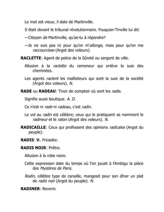
The screenshot in Figure 1.2 shows PyCharm, a popular IDE, aimed specifically at Python. The com-
munity version, which we use, is freely available from Jetbrains: https://www.jetbrains.com/
pycharm/download/. Other options are, e.g., VS Code and Atom, which support multiple program-
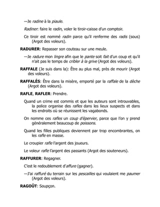
ming and typesetting languages either directly or through plugins. For scientific purposes a very popular
one is Spyder (see Figure 1.3), as it reminds many older users of the Matlab tool for scientific comput-
ing which they used before. Other features of Spyder include inspecting data arrays, plotting them and
many other advanced debugging tools.
22.
8 1. Gettingstarted
Figure 1.2: The PyCharm editor.
Figure 1.3: The Spyder editor.
Make sure to change the settings of file in the dialog box which will pop up the first time you run the file
to allow interaction with the Shell. Then you have similar features to which IDLE allows: checking your
variables in the shell after running your program or simply to testing a few lines of code.
Spyder has chosen to stop offering a standard Python console, so they only have an iPython console.
By tweaking the run setting per file, it is still possible to run your script in an external Python console.
But this would still be a reason to prefer PyCharm as it is more versatile and focused on Standard
Python applications not just the interactive iPython.
My advice would be to first keep it simple and use IDLE for the basics. Use the print() function and
the shell (to inspect variables) as debugger and occasionally www.pythontutor.com. Then later,
and only for larger or more complex problems switch to PyCharm or one of the multi-language IDE’s
(or optionally Spyder).
On the exam, only IDLE and Spyder will be available, unless specified otherwise in the course an-
nouncements.
A different environment especially for Scientific Computing, using iPython is Jupyter, which creates
23.
1.3. Installing Python9
Python Notebooks, a beautiful blend between a (LaTeX) document, spreadsheet and Python.
1.3.7. Documentation
IDLE, our default editor supplied with Python, has an option to Configure IDLE and add items to the
Help menu. Here a link to a file or a URL can be added as an item in the Help pull down menu.
The Python language documentation is already included,select them with F1, on-line they can be found
at
https://docs.python.org/3/
For Scipy and NumPy, downloading the .HTML files of the reference guides onto your hard disk and
linking to these files is recommended. They are available for download at:
http://docs.scipy.org/doc/
For Matplotlib both an online manual as well as a pdf is available at:
http://matplotlib.sourceforge.net/contents.html
Also check out the Gallery for examples but most important: with the accompanying source code for
plotting with Matplotlib:
http://matplotlib.sourceforge.net/gallery.html
For Pygame, use the online documentation, with the URL:
http://www.pygame.org/docs/
Another useful help option is entering ‘python’ in your favourite search engine, followed by what you
want to do. Since there is a large Python user community, you will easily find answers to your questions
as well as example source codes.
Other useful resources:
Search on Youtube for the course code AE1205 for some videos or the Python 3 playlist:
https://www.youtube.com/results?search_query=ae1205
Stackoverflow contains many answers and will often show up in your Google results: https://
stackoverflow.com/questions/tagged/python-3.x
A nice tutorial and reference can also be found at:
https://www.tutorialspoint.com/python3/index.htm
24.
10 1. Gettingstarted
1.4. Sneak preview: Try the Python language yourself
In the IDLE window, named Python Shell, select File > New Window to create a window in which you
can edit your program. You will see that this window has a different pull-down menu. It contains “Run”,
indicating this is a Program window, still called Untitled at first.
Enter (or copy) the following four lines in this window and follow the example literally.
Temperature conversion tool
print(”Temperature conversion tool”)
tempf = float(input(”Enter temperature in degrees Fahrenheit: ”))
tempc = (tempf - 32.0) * 5.0 / 9.0
print(tempf, ”degrees Fahrenheit is about”, round(tempc), ”degrees
Celsius”)
↪
Now select Run > Run Module. Depending on your settings, you might get a dialog box telling you
that you have to Save it and then asking whether it is Ok to Save this, so you click Ok. Then you enter
a name for your program like temperature.py and save the file. The extension .py is important for
Python, the name is only important for you. Then you will see the text being printed by the program,
which runs in the window named “Python Shell”:
Python shell output
>>>
Temperature conversion tool
Enter temperature in degrees Fahrenheit: 72
72.0 degrees Fahrenheit is about 22 degrees Celsius
>>>
Let’s have a closer look at this program. It is important to remember that the computer will step through
the program line by line. So the first line says:
print(”Temperature conversion tool”)
The computer sees a print() function, which means it will have to output anything that is entered
between the brackets, separated by commas, to the screen. In this case it is a string of characters,
marked by a ” at the beginning and the end. Such a string of characters is called a text string or just
string. When the computer prints this to the screen, it will also automatically add a newline character to
25.
1.5. Variables andthe assignment statement 11
jump to the next line for any next print statement (unless you specify otherwise, which will be explained
later).
This is all that the first line does. The next line is slightly more complicated, and will be analysed in the
next section.
Exercises section 1.4
Exercise 1.4.1: If you want to make it a bit more interesting, and harder for yourself, you could
make a variation on this program. In much the same fashion, you could try to make a saving/debt
interest calculator where you enter start amount, interest rate in percentage and number of years.
To raise x to the power y, you use x**y)
Exercise 1.4.2: Make a program that computes the overall resistance for the circuit shown below,
where your inputs are the three resistances (𝑅𝐴, 𝑅𝐵, 𝑅𝐶).
(Solutions to all exercises can be found in Appendix A)
1.5. Variables and the assignment statement
The second line in our temperature convertor is:
tempf = float(input(”Enter temperature in degrees Fahrenheit:”))
Different things are happening in this statement. The first part of the line, tempf =, is a so called
Assignment statement, indicated by the equals sign (=). It should be read as: “let tempf be”. In
general it has the following structure:
variablename = expression
In our example it tells the computer that in the computer’s memory a variable has to be created with
the name tempf. (If the variable name already exists, it will be just be overwritten by the result of the
expression at the end.)
To be able to do this, the computer first evaluates the expression on the other side of the “=” sign to
see what the type of this variable has to be. It could for example be a floating point value (float type)
or a round number (integer type), a series of characters (string) or a switch (boolean or logical). It then
reserves the required number of bytes, stores the type and the name. If the name already exists, then
this old value and type are cleared after the expression is evaluated.
The computer evaluates the expression. The outcome is stored in memory and can be used later
in other expressions by using the variable name on the left side of the equals sign. To do this, the
computer saves the name in a table associated with this module. This table contains information on
the type of variable and points to a computer memory address where the value is stored.
For the assignment statement a = 2, this table would look something like:
26.
12 1. Gettingstarted
name ’a’
type 4 byte Integer
memory address 1625981072
⋯ ⋯
Address Byte value
1625981072 0
1625981073 0
1625981074 0
1625981075 2
For numbers, three basic types of variables exist, each stored binary in a different way:
• Integers: 2
• Floats: 2.0
• Complex: 2.0+0j
Integers are whole numbers, used to count something or as an index in a table or grid. Floats are
numbers with a floating point and can have any real value. Complex numbers refer to the mathematical
definition of ‘complex’, which have a real part and an imaginary part. They are like floats but can have
an imaginary part next to the real part. Each type is stored in a different way.
Python looks at the expression to determine the type:
2 => integer type
-4 => integer type
3 * 4 => integer type
2.0 => float type
0. => float type
1e6 => float type
3 * 4.0 => float type
3 + 4j => complex type
In chapter 2 the assignment statement, as well as the different types of variables are discussed in
detail.
Now let us have a look at the expression in our example program. This is not a simple one. The
expression in our example has a combination of twice the following structure:
functionname(argument)
Python knows this is a function because of the parentheses. In our example case, there are two
functions: float() and input(). As the result of the input-function is needed as input of the float-
function, the input function is called first. In general, when functions are called in a nested way (a
function is placed inside of the parentheses of another function), the order of execution is from inside to
outside. Both float() and input() are standard functions included in the Python language. (Later
we will also use functions which we have defined ourselves!)
Most functions do some calculations and yield a value. For example, the abs(x) function returns the
absolute value (modulus) of x, and the function int(x) will try to convert the variable x to an integer
number. The int() function is one of the type conversion functions:
int(3.4) => integer with value 3
int(-4.315) => integer with value -4
float(2) => float with value 2.0
float(0) => float with value 0.0
But some functions are complete little programs in themselves. The input() function for example
does several things: it can be called with one argument (you can pass it a string with some text), which
will be printed on the screen, before the user is prompted to enter a value. When the user presses
enter, the value entered by the user is read, and this is returned in a string variable as the result by the
input function. So in our case, the text Enter temperature in degrees Fahrenheit: is printed, and the
27.
1.6. Finding yourway around: many ways in which you can get help 13
user enters something (hopefully a number). The text entered by the user is returned by input() as a
string, which in our example gets passed on to the float() function which tries to convert this string
to a floating-point value, to be stored in a memory location. We call this variable tempf.
The next line is again an assignment statement as the computer sees from the equal sign “=”:
tempc = (tempf - 32.0) * 5.0 / 9.0
Here a variable with the name tempc is created. The value is deduced from the result of the expression.
Because the numbers in the expression on the left side of the equals sign are spelled like “5.0” and
“32.0”, the computer sees we have to use floating point calculations. We could also have left out the
zero as long as we use the decimal point: 5. / 9. would have been sufficient to indicate that we want
to use floating point values.
Extra: Regular division and Integer division
When performing a division, we could also use only integers, so using 5 / 9. In Python 3, the
result of a division is always a float (this didn’t use to be the case in Python 2). Note that integer
division is available in Python: in this case two slashes are needed: 5 // 9 will return an integer.
Integer arithmetic always rounds down, so in this case the result would be zero. (See sections 2.4
and 2.5 for a detailed discussion on the difference between integers and floats).
When this expression has been evaluated, a variable of the right type (float) has been created and
named tempc, the computer can continue with the next line:
print(tempf,”degrees Fahrenheit is”,round(tempc),”degrees Celsius”)
This line prints four things: a variable value, a text string, an expression which needs to be evaluated
and another text string, which are all printed on the same line as with each comma a space character
is automatically inserted as well. The round() function means the result will be rounded off.
Try running the program a few times. See what happens if you enter your name instead of a value.
1.6. Finding your way around: many ways in which you can get
help
1.6.1. Method 1: Using help(”text”) or interactive help()
If you wonder how you could ever find all these Python-functions and function modules, here is how to
do that.
There are many ways to get help. For instance if you need help on the range function, in the Python
shell, you can type:
help(”range”)
Which calls the help-function and uses the string to find appropriate help-information. You can also
directly pass a function or other object to help:
help(list)
You can also use help interactively by typing help(), without arguments, and then type the keywords
at the “help>” prompt to get help, e.g. to see which modules are currently installed.
>>>help()
help>math
And you will see an overview of all methods in the math module. There are some limitations to this
help. When you will type append, you will not get any results because this is not a separate function
but a part of the list object, so you should have typed
28.
14 1. Gettingstarted
>>> help(list.append)
Help on method_descriptor in list:
list.append = append(...)
L.append(object) -- append object to end
1.6.2. Method 2: Python documentation in Help Pull-down menu
Another way to get help in Python is to use the supplied CHM-file, (compiled HMTL) via the Help-menu
of the IDLE-windows: Select Help>Python Docs and you will find a good set of documentation, which
you search in the “Index” or do a full text search (“Search”), see the following screenshots:
1.6.3. Method 3: Get help from the huge Python community
Python has a very large user community: conservative estimates say there are 3 to 5 million Python
users and it’s growing fast as MIT, Stanford and many others use Python in their programming courses
and exercises. It is also the most popular language among PhDs. IEEE calls it the standard language
for scientific computing and data analysis.
So simply Googling a question (or error message) with the keyword Python (or later NumPy) in front
of it as an extra search term will quickly bring you to a page with an example or an answer. For basic
questions this might bring you to the same documentation as in the Help-menu which is at https://
docs.python.org. You will also see that https://www.stackoverflow.com is a site that often
pops up, and where most questions you might have, have already been posed and answered:
29.
1.6. Finding yourway around: many ways in which you can get help 15
For instance, for the search query “python append to a list” you will find: https://stackoverflow.
com/questions/252703/python-append-vs-extend (Which shows that next to append()
there apparently is another method called extend() available, which works with a list as an argu-
ment and apparently appends each element to the list.)
In general, thanks to the interactive Python Shell window, simply trying statements or program lines in
the Python shell is a way to try what works as you intended. Or to check the value of variables after
your still incomplete program has run.
To find bugs in your program, for small programs https://www.pythontutor.com can be helpful
to see what is going on inside the computer when your program runs. And of course using the print
statement to see what a variable is, or where the computer gets stuck in your program, is always the
first thing to try.
Be prepared that in the beginning the level of frustration might be high, but so is the reward when your
program runs. And when you get experience, you will see how fast you can make working programs,
not because you won’t create bugs, but because you will immediately recognise what went wrong. The
nice thing of software is that it can always be fixed, so “trial and error” is an accepted way to develop
programs. So do not be afraid to try things and play around with Python to get acquainted with the way
it works.
Appendix C gives an overview of all of the Python statements and most important functions that are
covered in this course, with a short example for each item. Having a copy of these pages at hand may
be handy when starting Python. It will provide the keywords for you to look into the help-functions of
Google searches.
Although we already touched upon most basic elements of the Python language, we have not seen all
statements and types yet, so first go through the next chapters (discover the very useful while-loop, the
string type and its methods and the Boolean/logical and slicing of strings and lists etc.). Just glance over
these chapters to get the essence and then start making simple programs and study the paragraphs in
more detail when you (think you) need them. Programming has a steep learning curve at the beginning,
so good luck with making it through this first phase. Once you have passed this, things will be a lot
easier and more rewarding. Good luck!
31.
2
Variable assignment andtypes
In this chapter we describe the building blocks which you need to write a program. First we have a look
at variables, which represent the way in which a computer stores data. But there are different types
of data: numbers or bits of text for instance. There are also different kinds of numbers, and of course
there are more data types than just text and numbers, like switches (called “booleans” or “logicals”)
and tables (“lists”). The type of variable is defined by the assignment statement; the programming line
giving the variable its name, type and value. Therefore we first concentrate the assignment statement
and then the different data types are discussed.
In this reader we’ll often use examples to introduce and explain programming concepts. The example
we’ll start out with in this chapter is a program to solve a second order polynomial equation. We will
use this example to discuss the use of variables in systematic fashion.
ABC solver
import math
print(”To solve ax2 + bx + c = 0 :”)
a = float(input(”Enter the value of a: ”))
b = float(input(”Enter the value of b: ”))
c = float(input(”Enter the value of c: ”))
D = b ** 2 - 4.0 * a * c
x1 = (-b - math.sqrt(D)) / (2.0 * a)
x2 = (-b + math.sqrt(D)) / (2.0 * a)
print(”x1 =”, x1)
print(”x2 =”, x2)
Before we start some notes about this program. Run this program and you will see the effect.
• note how ** is used to indicate the power function. So 5 ** 2 will yield 25, and 16 ** 0.5
will yield 4.
• the program uses a function called sqrt(); the square root function. This function is not a
standard Python function. It is part of the math module, supplied with Python. When you need
functionality of such external modules in your code, you can use the import statement at the
beginning of your code to make these modules accessible. The expression math.sqrt() tells
Python that the sqrt() function should be obtained from the imported math module. You’ll learn
more about using modules in chapter 5.
17
32.
18 2. Variableassignment and types
• After you have run the program, you can type D in the shell to see the value of the discriminant.
All variables can be checked this way.
• Note the difference between text input and output. There is no resulting value returned by the
print function, while the input function does return a value, which is then stored in a variable.
The argument of the input-function calls is between the brackets: it’s a prompt text, which will be
shown to the user before he enters his input.
2.1. Assignment and implicit type declaration
A variable is a reference by name to a memory location with a value and a type. You define a variable
when you assign a value or expression to it. This expression also determines the type. The assignment
statement is very straightforward:
variablename = expression
Example assignment statements for the four main types (which will be discussed in detail in the following
sections):
Integers, only whole numbers, using digits and the sign:
Integers
i = 200
a = -5
Floats, contain a decimal point or “e” to indicate the exponent of the power of 10:
Floating point values
inch = 2.54
ft = .3048
lbs = 0.453592
spd = 4.
alt = 1e5
Logicals:
Logicals
swfound = True
alive = False
forward = (v > 0.0)
onground = h <= 0.0 and abs(v) < eps
running = (forward or alive) and not onground
Strings (starting and ending with single or double quotes):
Strings
name = ”Ian ” + ”McEwan”
txt = ”I'm afraid I can't do that, Dave.”
s = 'HAL'
Python even allows multiple assignments in a single line, when the values are separated by a comma:
a, b, c = 1.0 , 3.0 , 5
a, b = b, a # swap two variables
What really happens is that the expression first becomes a type of list (a tuple to be exact) which is
then unpacked. The example below shows that this principle also works with a list, which is defined by
a series of variables within square brackets:
33.
2.2. Short-hand whenusing original value with an operator 19
lst = [9 , 2 , 5]
a, b, c = lst
2.2. Short-hand when using original value with an operator
The “=” in an assignment means: “make equal to”. To increase the integer variable i with one, we
normally type:
i = i + 1 # increase i with one
Mathematically speaking this statement would be nonsense if we would read the equal sign as ‘being
equal to’. But as an assignment statement, this simply evaluates the expression on the right side, which
is the content of variable i to which one is added, and the result is stored in the variable i again. The
effect is thus that i is increased with 1. Here are a few other example with the same logic:
j = j - 1 # decrease j with one
n = n * 2 # doubles n
x = x / 2 # halves x
a = a * k # a will be multiplied by k
As especially the increase or decreases with one occurs often, there is a shorthand notation for things:
i = i + => i +=
So the examples above can also be coded like this:
i += 1 # increase i with one
j -= 1 # decrease j with one
n *= 2 # doubles n
x /= 2 # halves x
a *= k # a will be multiplied by k
This short-hand is the same as in the programming language C (and C++), a language which is well
known for how short code can be written (often with an adverse effect on the readability). Also in this
example, the benefit is mainly for the programmer who saves a few keystrokes, (in Python) there is
no execution time benefit as the operations done are the same. This short-hand hence increases the
distance from pseudo-code. Whether you use it is a matter of personal preference.
2.3. Number operations in Python
For the number types float, integer (and complex) the following operators can be used
+ Addition
- Subtraction
* Multiplication
/ Division
// Floored or integer division (rounded off to lower round number)
% Modulo, remainder of division
** Power operator x**y is x to power y, so x**2 is x2
-x Negated value of x
+x Value of x with sign unchanged
As well as the following standard functions:
abs(x) Absolute value of x; |x|
pow(x, y) Power function, same as x ** y
divmod(x, y) Returns both x // y and x % y
34.
20 2. Variableassignment and types
2.4. Float: variable type for floating point values
Floating point variables, commonly referred to as floats, are used for real numbers with decimals. These
are the numbers as you know them from your calculator. Operations are similar to what you use on a
calculator. For power you should use the asterisk twice, so 𝑥𝑦
would be x ** y.
They are stored in a binary exponential way with base 2 (binary). This means that values which are
round values in a decimal systems sometimes need to be approximated. For instance if you try typing
in the shell:
>>> 0.1 + 0.2
The result will be:
>>> 0.1 + 0.2
0.30000000000000004
Often this is not a problem, but it should be kept in mind, that float are always approximations!
One special rule with floats in programming is that you never test for equality with floats. So never
use the condition “when x is equal to y” with floats, because a minute difference in how the float is
stored can result an inaccuracy, making this condition False when you expected otherwise. This may
not even be visible when you print it, but can still cause two variables to be different according to
the computer while you expected them to be the same. For example: adding 0.1 several times and
then checking whether it is equal to 10.0 might fail because the actual result is approximated by the
computer as 9.99999999 when it passes the 10. So always test for smaller than (<) or larger than (>).
You can also use “smaller or equal to” (<=) and “larger or equal to” (<=), but do not forget that a floating
point variable is always an approximation due to the binary storage limitations (which is different from
a decimal notation), so it may be off by a small value. A way to avoid it is to test for closeness:
Closeness test of a float
# Test for equality with floats
eps = 1e-7 #value depends on scale you’re looking at
if abs(x - y) < eps:
print(”x is equal to y”)
Floating point values can also be rounded off using the round(x) or round(x, n) function. With
the second argument n, you can specify the number of decimals. When the second argument is not
used, the result will be rounded off to the nearest whole number and converted to the type integer
automatically.
>>> round(10 / 3)
3
>>> round(10 / 3, 4)
3.3333
>>> round(10 / 3, 0) # Explicitly specify zero decimals lets round
return a float
↪
3.0
Extra: Try for yourself
Try adding 0.1 to a variable for more than 1000 times (use a for-loop or while-loop) and check the
variable value to see this effect.
2.5. Int: variable type for round numbers like counter or index)
Integers are variables used for whole numbers. They are used for example as counters, loop variables
and indices in lists and strings. They work similar to floats but division results will be of the type float.
35.
2.5. Int: variabletype for round numbers like counter or index) 21
For example:
a = 4
b = 5
c = a / b
d = a // b
print(c)
print(d)
In this example, the first print statement will print 0.8, but the second statement prints 0. The difference,
as mentioned before, is the difference between regular division (/) and integer division (//). The former
returns a float, whereas the latter returns an integer. Note also that with integer division, the result is
always rounded down.
A useful operator, commonly used with integers, is the ‘%’ operator. This operator is called the modulo
function, and calculates the remainder of a division. For example:
27 % 4 = 3
4 % 5 = 4
32 % 10 = 2
128 % 100 = 28
So to check whether a number is divisible by another, checking for a remainder of zero is sufficient:
if a % b == 0:
print(”a is a multiple of b”)
You can convert integers to floats and vice versa (since they are both numbers) with the functions
int() and float():
a = float(i)
j = int(b) # Conversion cuts of behind decimal point
k = int(round(x)) # Rounded off to nearest whole number
# ..and then converted to an integer type
The int() function will cut off anything behind the decimal point, so int(b) will give the largest integer
not greater than b (in other words, it rounds down). These functions int() and float() can also
take strings (variables containing text) as an argument, so you can also use them to convert text to a
number like this:
txt = ”100”
i = int(txt)
a = float(txt)
Note the different functions related to division in the example below:
n = 20
i = 3
a = n / i
print(”a =”,a)
j = n // i # floor division
k = int(n / i) # rounded down and converted to int
m = round(n / i) # rounded to nearest integer value
print(”j,k,m =”, j, k, m)
The output of this program will be:
36.
22 2. Variableassignment and types
a = 6.666666666666667
j,k,m = 6 6 7
As we can see from the missing decimal points in the second output line, the variable j, k, m all are
integers. This can also be verified in the shell using the type() function, which prints the type of a
variable:
>>> type(m)
<class 'int'>
2.6. Complex numbers
Python has complex numbers built-in as a standard type. In many other languages one would have to
treat this as two float numbers, the real part and the imaginary part, but in Python the j directly after a
number signals an imaginary art and will change the resulting type to complex.
c = 3 + 4j
print (”Length of”, c, ”is”, abs(c))
Will give the following output:
Length of (3+4j) is 5.0
To access the different components, use the following method:
c = 3 + 0j
a = c.real
b = c.imag
print(”c has”, a, ”as real part and”, b, ”as imaginary part”)
Will give the following output:
c has 3.0 as real part and 0.0 as imaginary part
All other operations work as expected:
>>> e = 2.718281828459045
>>> pi = 3.141592653589793
>>> e ** (1j * pi)
(-1+1.2246467991473532e-16j)
Which demonstrates Euler’s equation, and also shows the rounding off problems in the imaginary part,
which is practically zero. Both e and pi were binary approximations, as are all floats and complex
numbers.
2.7. String operations
Strings are variables used to store text. They contain a string of characters (and often work similar to
a list of characters). They are defined by a text surrounded by quotes. These quotes can be single
quotes or double quotes, as long as you use the same quote-character to start and end the string. It
also means you can use the other type of quote-symbol inside the text. A useful operator on strings is
the “+” which glues them together. This can be very useful, e.g., in functions which expect one string
variable (like the input function). Example string assignments:
txt = ”abc”
s = ””
37.
2.8. Booleans andlogical expressions 23
name = ”Graham” + ”Chapman” # (so the + concatenates strings)
words = 'def ghi'
a = input(”Give value at row” + str(i))
Some useful basic functions for strings are:
len(txt) returns the length of a string
str(a) converts an integer or float to a string
eval(str) evaluates the expression in the string and returns the number
chr(i) converts ASCII code i to corresponding character (see table 2.1)
ord(ch) returns ASCII code of the character variable named ch
Using indices in square brackets [ ] allows you to take out parts of a string. This is called slicing. You
cannot change a part of string but you can concatenate substrings to form a new string yielding the
same effect:
c = ”hello world”
c[0] is then ”h” (indices start with zero)
c[1:4] is then ”ell” (so when 4 is end, it means until and not including 4)
c[:4] is then ”hell”
c[4:1:-1] is then ”oll” so from index 4 until 1 with step -1
c[::2] is then ”hlowrd”
c[-1] will return last character ”d”
c[-2] will give one but last character ”l”
c = c[:3] + c[-1] will change c into ”hel” + ”d” = ”held”
The string variable also has many functions built-in, the so-called string methods. See some examples
below (more on this in chapter 8).
a = c.upper() returns copy of the string but then in upper case
a = c.lower() returns copy of the string but then in lower case
a = c.strip() returns copy of the string with leading and trailing spaces removed
sw = c.isalpha() returns True if all characters are alphabetic
sw = c.isdigit() returns True if all characters are digits
i = c.index(”b”) returns index for substring in this case “b”
For more methods see chapter 8, or section 5.6.1 of the Python supplied reference documentation in
the Help file.
Strings are stored as lists of characters. Internally, Characters are stored by the computer as numbers,
using the Unicode encoding. This encoding is an extension of the ASCII codes. See table 2.1:
ASCII codes can be derived from the corresponding character using the ord(char) function. Similarly,
the character for a given ASCII code i can be retrieved using the chr(i) function. As you may
have noticed in table 2.1, the first 31 and the last entry are ‘special’ characters. Most of these special
characters you will likely never need. Exceptions to this are the newline character, and the tab character.
These special can be easily entered into a string using an ‘escape character’: a backslash followed
by a character. In this way, you can add a newline to a string by adding 'n', and a tab by adding
't'. When you start reading text files from disk (see chapter 8), you might notice that newlines can
also be indicated with other characters: In Windows/DOS text files the newline is indicated by both
a Carriage Return and a Line Feed: chr(13) + chr(10). On Linux and Apple systems only the
newline character chr(10) is used.
2.8. Booleans and logical expressions
Booleans (or logicals) are two names for the variable type in which we store conditions. You can see
them as switches inside your program. Conditions can be either True or False, so these are the only
two possible values of a logical. Mind the capitals at the beginning of True and False when you use
these words: Python is case sensitive. Examples of assignments are given below:
38.
24 2. Variableassignment and types
0 NUL (Null) 32 SP 64 @ 96 ‘
1 SOH (Start of Header) 33 ! 65 A 97 a
2 STX (Start of Text) 34 ” 66 B 98 b
3 ETX (End of Text) 35 # 67 C 99 c
4 EOT (End of Transmission) 36 $ 68 D 100 d
5 ENQ (Enquiry) 37 % 69 E 101 e
6 ACK (Acknowledgement) 38 & 70 F 102 f
7 BEL (Bell) 39 ' 71 G 103 g
8 BS (Backspace) 40 ( 72 H 104 h
9 HT (Horizontal Tab) 41 ) 73 I 105 i
10 LF (Line Feed) 42 * 74 J 106 j
11 VT (Vertical Tab) 43 + 75 K 107 k
12 FF (Form Feed) 44 , 76 L 108 l
13 CR (Carriage Return) 45 - 77 M 109 m
14 SO (Shift Out) 46 . 78 N 110 n
15 SI (Shift In) 47 / 79 O 111 o
16 DLE (Data Link Escape) 48 0 80 P 112 p
17 DC1 (Device Control 1 (XON)) 49 1 81 Q 113 q
18 DC2 (Device Control 2) 50 2 82 R 114 r
19 DC3 (Device Control 3 (XOFF)) 51 3 83 S 115 s
20 DC4 (Device Control 4) 52 4 84 T 116 t
21 NAK (Negative Acknowledgement) 53 5 85 U 117 u
22 SYN (Synchronous Idle) 54 6 86 V 118 v
23 ETB (End of Transmission Block) 55 7 87 W 119 w
24 CAN (Cancel) 56 8 88 X 120 x
25 EM (End of Medium) 57 9 89 Y 121 y
26 SUB (Substitute) 58 : 90 Z 122 z
27 ESC (Escape) 59 ; 91 [ 123 {
28 FS (File Separator) 60 < 92 124 |
29 GS (Group Separator) 61 = 93 ] 125 }
30 RS (Record Separator) 62 > 94 ^ 126 ~
31 US (Unit Separator) 63 ? 95 _ 127 DEL
Table 2.1: The ASCII table.
found = False
prime = True
swlow = a < b
outside = a >= b
swfound = a == b
notfound = a != b # ( != means: not equal to)
outside = x < xmin or x > xmax or y < ymin or y > ymax
inside = not outside
out = outside and (abs(vx) > vmax or abs(vy) > vmax)
inbetween = 6.0 < x <= 10.0
Conditions are a special kind of expression used in statements like if and while to control the flow
of the execution of the program. In the above statements, often brackets are used to indicate that it is
a logical expression.
NB: Testing equality vs assignment
To test whether two variables are the same, you have to use two equals signs (==). This is easily
confused with the assignment statement, which uses a single equals sign (=)! In most cases, when
you confuse these two, your program will still run, but the results will obviously not be what you
39.
2.9. The listtype: an ordered collection of items 25
expect! So remember: Two equals signs will check the condition and one equals sign assigns an
expression to a variable name.
Extra: Alternative syntax for ‘not equal to’
For “is not equal to” both != as well as <> can be used, but != is preferred.
With combined conditions with many “and”, “or” and “not” statements use brackets to avoid confu-
sion:
not((x > xmin and x < xmax) or (y > ymin and y < ymax))
You can use logicals as conditions in if and while statements:
if inside:
print(”(x,y) is inside rectangle”)
while not found:
i = i + 1
found = (a == lst[i])
Note that if inside basically means: if inside == True and similarly while not found
means while found == False. This is why Booleans are never compared with True or False as
this serves no function (for more information on if-statements, see section 3.4, for while-statements,
see section 3.6).
2.9. The list type: an ordered collection of items
2.9.1. What are lists?
Lists are a way to group variables together. This allows you to repeat something for all elements of a list
by using an index as a counter or by iterating through the list with the for-statement (see section 3.5).
This could be a repetitive operation, but also a search or a sorting action. Often it is useful to have a
series of variables that are grouped together. You can therefore look at a list as if it is a table. Each
element of a list can be of any type: it can be an integer, float, logical, string or even a list! Special for
Python is that you can even use different types in one list; in most programming languages this would
not be possible. Both to define a list, as well as to specify an index, square brackets are used as in
strings:
Creating lists
a = [2.3 , 4.5 , -1.0, .005, 2200.]
b = [20, 45, 100, 1, -4, 5]
c = [”Adama”, ”Roslin”, ”Starbuck”, ”Apollo”]
d =[[”Frederik”,152000.0], [”Alexander”,193000.0],
[”Victor”,110000.0]]
e = []
This would make the variable a a list of floats, b a list of integers, and c a list of strings. A list of lists
as defined in d is basically a way to create a two-dimensional list. Finally e is an empty list. Accessing
elements from the list is done as indicated below. Another way to make a list of numbers is using the
so-called range function. This is a so-called iterator function used primarily in loops, but it can also be
converted to a list. The range function can contain one two or even three arguments:
range(stop)
range(start, stop))
range(start, stop, step))
40.
26 2. Variableassignment and types
In all these cases start is the start value (included), stop is the value for which the block is not
executed because for will stop when this value is reached. So it is an inclusive start but excludes stop.
Another option is to enter a third argument, to indicate a stepsize. The default start is 0, the default
step is 1. Note that range() only works with integers as arguments:
list(range(5)) gives [0, 1, 2, 3, 4]
list(range(5,11)) gives [5, 6, 7, 8, 9, 10]
list(range(5,11,2)) gives [5, 7, 9]
2.9.2. Indexing and slicing, list functions and delete
Let’s use the following list:
lst = [1, 2, 3, 4, 5, 6, 7, 8, 9, 10]
If we now print elements we can use the indices in many ways. Using one index, indicating a single
element:
lst[0] which holds value 1
lst[1] which holds value 2
lst[9] which holds value 10
lst[-1] last element, which holds the value 10
lst[-2] one but last element which holds the value 9
Here it can be seen that indices start at 0, just as with strings. And similar to strings, the function len()
will give the length of a list and thus the not to reach maximum index for the list. Slicing lists with indices
works in the same way as it does for strings, with three possible arguments: start, stop and step. Only
one index refers to one single element. Two arguments separated by a colon refer to start and stop. A
third can be used as step. If you look at the lists that were made in the previous paragraph about lists
you can see that:
a[1] will return a float 4.5
b[1:4] will return a list [45, 100, 1]
d[1][0] will return ”Alexander” (do you see the logic of the order of the in-
dices for the different dimensions: second element of main list, then first
element of that list?)
Adding and removing elements to a list can be done in two ways: the “+” operator, or the append and
extend functions:
a = a + [3300.0] will add 3300.0 at the end of the list
a = a[:-2] will remove the last two elements of the list (by first copying
the complete list without the last two elements, so not very
efficient for large lists)
a = a[:i]+a[i+1:] will remove element i from the list, when it’s not the last one
in the list
a = b + c will concatenate (glue together) two lists if b and c are lists
Another way is to use the del (delete command) and/or functions which are a part of the list class.
You call these functions using the dot notation: variablename.functionname() so a period be-
tween variablename and functionname. Some examples:
a.append(x) add x as a list element at the end of the list named a, equiva-
lent to a = a + [x]
a.extend(b) extend the list with another list b, equivalent to a = a + b
a.remove(3300.0) removes the first element with value 3300.0
del a[-1] removes the last element of a list named a
del a[3:5] removes the 4th till the 6th element of a list named a
a = a[:3] + a[4:] will remove the 4th element of the list named a
Slicing
41.
2.9. The listtype: an ordered collection of items 27
The last example line uses the slicing notation (which can also be used on strings!). Slicing, or cutting
out parts of a list is done with the colon notation. Slicing notation is similar to the range arguments:
start:stop and optionally a step can be added as third argument: start:stop:step. If no value
is entered as start, the default value is zero. If no value is added as end the default value is the last
element. The default step size is 1. Negative values can be used to point to the end (-1 = last element,
-2 is the one-but-last, etc.).
Using the original definition of the lst variable: lst = [1, 2, 3, 4, 5, 6, 7, 8, 9, 10],
this will give:
lst[:3] first three element index 0,1,2: [1,2,3]
lst[:-2] all except last two elements
lst[4:] all elements except the first four: except elements nr 0,1,2,3
lst[::2] every second element so with index 0,2,4, until the end
Other useful functions for lists:
b.index(45) will return the index of the first element with value 45
len(d) will return the length of the list
min(a) will return the smallest element of the list variable a
max(a) will return the largest element of the list variable a
sum(a) will return the sum of the elements in the list variable a
2.9.3. Quick creation of lists with repeating values
If you need to create a one-dimensional list with multiple times the same value, Python offers the
following short-hand:
a = 5 * [0]
print(a) # Would print [0, 0, 0, 0, 0]
a[1] = 1
print(a) # Would print [0, 1, 0, 0, 0]
This notation, however, does not work for nested (two-dimensional) lists. When you need this, you can
use a loop to construct your list:
a=[]
for i in range(3):
a.append(3*[0])
a[0][1] = 1
print(a) # Would print [[0, 1, 0], [0, 0, 0], [0, 0, 0]]
This is a safe way of constructing nested lists, as each new element of a is constructed from scratch.
The following would also work:
# if your list is small, just do it entirely by hand
a = [[0, 0], [0, 0], [0, 0]]
# You can also initialise your list with dummy values, which you replace
afterwards:
↪
a = [0, 0, 0]
for i in range (3):
a[i] = [0, 0]
If you are not sure, test a simple example by constructing your nested list, changing one of its elements,
and see the effect by printing the entire list. You can also use www.pythontutor.com to visualise
what is going on in the computer’s memory. In the above example we use a for-loop to execute a line
of code a fixed (in this case 3) number of times. You’ll learn more about for-loops in section 3.5.
42.
28 2. Variableassignment and types
Extra: The tricky nature of mutable types
Although the short-hand notation described above doesn’t give you what you’d expect, it doesn’t
return an error either. What happens is the following:
a = 3 * [3 * [0]]
print(a) # Would print [[0, 0, 0], [0, 0, 0], [0, 0, 0]]
a[0][1] = 1
print(a) # Would print [[0, 1, 0], [0, 1, 0], [0, 1, 0]]
The result of the second print statement is probably not what you expected! In line 3 we only
change the second element of the first row, but surprisingly all rows (all lists) have their second
element changed into 1!
What happens is related to the fact that some types are mutable (lit. ‘can be changed’), and others
immutable (lit. ‘cannot be changed’). In Python, all basic types, like floats, integers, and booleans
are immutable. So in the following, variable a is copied into b:
a = 1 # Create an integer variable in memory, with value 1
b = [a, a, a] # Create a list, with three copies of a as content
However, aggregate types (i.e., combinations of multiple data, such as a list) are mutable, which
in Python means that they are passed by reference. This results in the following:
a = [0, 0] # Create a list
b = [a, a, a] # Create a second list, with three references to a as
content
↪
Here, b literally contains three times the original variable a. Changing the contents of a therefore
results in the same behaviour as the short-hand construction of nested lists:
a[0] = 1
print(b) # Would print [[1, 0], [1, 0], [1, 0]]
Have a look at this Python-tutor example for a visualisation of such construction and referencing!
2.9.4. List methods
Another powerful attribute of Python’s list is the number of methods that come with it. Methods are
functions which you call with the dot-notation, as you already saw in section 2.9.2, and in the previous
section with the append() method. An example of this is the sort method:
a = [2, 10, 1, 0, 8, 7]
a.sort()
print(a) # Would print [0, 1, 2, 7, 8, 10]
As we can see the method sort() (you can recognise functions and methods by the presence of
parentheses) sorts the list a. This is a special function in that it changes the actual source list instead
of creating a sorted copy (this is called an in-place operation). Most methods will return the result of
the function as a new variable, and leave the original intact. Examples are the methods index and
count. Index will give the index of the first occurrence of the given value. Count will give the total
number of occurrences:
>>> a = [3,1,8,0,1,7]
>>> a.count(1)
2
>>> a.index(1)
1
43.
2.10. Some usefulbuilt-in functions 29
>>> a.index(9)
Traceback (most recent call last):
File ”<pyshell#23>”, line 1
a.index(9)
ValueError: 9 is not in list
>>>
How would you make a program which will print the index of the first occurrence but also avoids the
error message if it is not found by simply printing -1?
Exercises section 2.9
Exercise 2.9.1: Make a program which calculates effect of a yearly interest rate (entered by the
user) on start sum (also entered by the user). Print the amount after each year (ask the user how
many years).
Exercise 2.9.2: Make a list of words input by the user (e.g. aeroplane company names) by using
the append() function, then print them below each other with the length of each word.
Exercise 2.9.3: You can also make a list which consists of different lists, each with a different
length, as shown here:
values = [[10, 20], [30, 40, 50, 60, 70]]
Print the length of each list and all the values it contains.
Exercise 2.9.4: We can also go in the other direction, and construct a list of lists from a list of
values and a list of lengths:
values = [10, 20, 30, 40, 50, 60, 70] lengths = [2, 2, 3]
Construct a list of lists, with each list i containing lengths[i] values from values. Print the
constructed list.
2.10. Some useful built-in functions
As we have already seen in the examples, Python has a number of built-in functions which you can
use in the right side of assignment statements on any expression using values and variables:
float(i) converts an integer or string(text) to a float
int(x) converts a float to an integer (whole number rounded to
lowest integer)
round(x) rounds off to nearest round number and converts to in-
teger
round(x,n) rounds off a float n decimals, result is still float
str(x) converts a number into a string (text)
eval(txt) converts a text to a number
bool(x) convert x to a Boolean (typically non zero is True)
repr(x) generates a string with a printable content of x
list(txt) converts x to a list type (e.g. splits string in single char-
acters)
chr(i) gives character for ascii code i (look up ascii table to see
codes)
ord(c) gives acsii code of character c (a string with length one)
len(txt) gives length of the string txt
len(lst) gives length of the list lst
abs(x) absolute value of x (modulo/length for complex numbers)
range(stop) give a list [0,1,...stop-1] so stop is not included
44.
30 2. Variableassignment and types
range(start,stop) give a list [start, start+1,...,stop-1] so start is included!
range(start,stop,step) give a list [start, start+step,...] stop is not included
sum(a,b,c,d,...) total sum of variables a,b,c,d,...
sum(lst) total sum of the list elements in lst
max(a,b,c,d,...) maximum value of a,b,c,d,...
max(lst) maximum value in the list lst
min(a,b,c,d,...) minimum value of a,b,c,d,...
min(lst) minimum value in the list lst
input(txt) prints txt, asks user for input, returns user input as a text
string
help(txt) for use in shell: prints help on Python or installed
function, module or statement, e.g. help(’math’) or
help(’input’)
45.
3
Python syntax: Statements
3.1.Assignment
In this chapter we discuss the basic Python statements: commands that you use in a program which
often do something with the data. A summary of all of the basic python statements covered in this
course can be found in Appendix C.
We already discussed the assignment statement at the beginning of the previous chapter. The assign-
ment statement is one of the simplest statements in Python:
Ë Ê
variablename = expression
This general statement is executed in the following order:
1. Evaluate expression, and store the result in memory
2. Point variablename to the area of memory created in step 1.
The type and value of the variable variablename is determined by the expression.
Note that it is possible to overwrite a variable, even when it is used in the expression on the right-hand
side of the equals sign. This is because the computer first evaluates the expression and only then
stores the result in the variable, overwriting anything that was previously stored in that variable.
Some examples of how you can use the assignment are given below:
a = 4.5 will: (1) create a float with value 4.5, and (2) point variable
name a to it
i = 100 will: (1) create an integer with value 100, and (2) point variable
name i to it
total = 0 will: (1) create an integer with value 0, and (2) point variable
name total to it
i = i + 1 will: (1) calculate the result of i + 1, store it in a new integer,
and (2) point variable name i to it
i += 1 equal to previous line
total = total + i will: (1) calculate the result of total + i, store it in a new
integer, and (2) point variable name i to it
total += i equal to previous line
txt = ”ea” will: (1) create a string containing ”ea”, and (2) point variable
name txt to it
31
46.
32 3. Pythonsyntax: Statements
txt = txt + ”sy” will: (1) evaluate the expression txt + ”sy”, store the result
(”easy”) in a new string, and (2) point variable name txt to
it
series = [] will: (1) create an empty list, and (2) point variable name se-
ries to it
series = series + [i] will: (1) create a new list, containing the contents of series,
appended with an additional element i, and (2) point variable
name series to it
Here it should be noted that a statement such as i = i + 1 may seem mathematically incorrect,
but in programming this simply means that the expression i + 1 is evaluated with the old value of
i, after which the variable i is updated to point to the result of the expression. This order of actions
basically means that ‘=’ means ‘will become’ instead of ‘is equal to’ (remember that for the ‘is equal
to’ comparison ‘==’ in Python). Also note the short-hand notation “+=”, which has been discussed
extensively in section 2.1 already.
Adapting our example program from the previous chapter, we add some logic. Edit the program to
match this example precisely, note the margin jumps (use TAB-key) in the if statement, which is
called indentation. Having the same margin, or indentation level, is what Python uses to mark blocks
of code that belong together, for example because they are part of an if-branch or a loop (see later
sections on for and while loops).
ABC solver with discriminant check
from math import sqrt
print(”To solve ax2 + bx + c = 0 :”)
a = float(input(”Enter the value of a: ”))
b = float(input(”Enter the value of b: ”))
c = float(input(”Enter the value of c: ”))
D = b ** 2 - 4.0 * a * c
if D < 0.0:
print(”This equation has no solutions”)
else:
x1 = (-b - sqrt(D)) / (2.0 * a)
x2 = (-b + sqrt(D)) / (2.0 * a)
print(”x1 =”, x1)
print(”x2 =”, x2)
Now the program first checks whether D is negative. If so, it will tell you that there are no solu-
tions.
• Note the structure and syntax(=grammar) of the if-else statement. A colon ( : ) indicates that
a block of code will be given, so it acts as a ‘then’. The block is marked by the increased level of
indentation of the code.
• When it jumps back to the margin of the beginning to indicate the end of this block of code, an
‘else’ follows, again with a colon and an indented block of code.
• It also uses a different way to import the sqrt function from the math module. Note the dif-
ference in syntax in both the line with the import statement as well as the line where the sqrt
function is used. Chapter 5 will explain the different ways to import modules.
47.
3.2. The printstatement 33
Exercises section 3.1
Exercise 3.1.1: Adapt the program so that it calculates the hypotenuse c of a rectangular triangle
for rectangular sides a and b as entered by the user, using Pythagoras formula.
Exercise 3.1.2: Using the flow chart depicted below, make a program that determines the
maximum value of given numbers a, b, c and d as entered by the user, using a number of if-
else-statements to find the maximum value of these four variables.
start
Enter values
a, b, c, d
a > b?
max1 = a max1 = b
c > d?
max2 = c max2 = d
max1 > max2?
end
print max1 print max2
Exercise 3.1.3: Write a program that clamps a float input by the user to [-10, 10] and prints it.
Additionally, if the input is negative, the program should print a warning message.
3.2. The print statement
The print function generates text output in the console. It can print text, variables and (the result
of) expressions. To print several things on one line, pass them to the print function, separated by
commas. In the resulting printed line of text, a space will automatically be inserted between each
argument. The space is the default so-called ‘separator’ symbol. After each call to print automatically
a newline character is printed, so the next print call will start at a new line. A print-statement without
any arguments, prints an empty line, or a newline character to be exact.
3.2.1. Using print
Below is an example of four different ways of using the print command, which will result in exactly
the same output (printing the text ‘Hello world’ to the console, followed by a newline):
# Method 1
print(”Hello world”)
# Method 2
print(”Hello”, ”world”, sep=” ”)
# Method 3
48.
34 3. Pythonsyntax: Statements
print(”Hello”, ”world”, end=”n”)
# Method 4 (using two print statements)
print(”Hello”,end=” ”)
print(”world”)
The above examples also use the use of the ‘sep’ and ‘end’ keyword, which can be used to use a
different separator character or a different end of line. Note how the hash symbol (#), indicates the
start of a comment: this symbol and everything after it is ignored by the Python interpreter when the
program is executed.
The print statement can print one or more texts, variables expressions and the outcome of functions.
Basically anything can be printed. Apart from generating output for the user, print is also very useful
when trying to find bugs in your program. Experienced programmers often put temporary print state-
ments after every so many lines of code to check if everything works as intended. These are then later
deleted or commented out with the hash symbol.
Other examples of valid print statements with other arguments than strings:
print(”Program to solve 2nd order equations. ”)
print(”The solutions are”, x1, ”and”, x2)
print(”Discriminant is”, b * b - 4.0 * a * c)
print(”List of names”, lst)
print()
print(”Ready. ”)
Extra: Using print to output to a file
Next to ‘sep=’ and ‘end=’, there is also the keyword ‘file=’, which can be used to print to a file
instead of to the screen (see chapter 8 for more information on how to read and write text files).
This file needs to be opened first with the open function. This function returns a file-object. The
next example shows how this can be used to print to:
# Open file for writing (see ch 8)
fout = open('test.dat','w')
print(”abc”, file=fout)
print(”def”, file=fout)
f.close() # Close file
3.2.2. Formatting your output
Sometimes more control is needed over how data is printed, or stored in a string of text. For instance
how many decimals are printed or to line up a series of numbers using the decimal point in a more
table-like fashion. Or when you want to right-align a number of integers, or add leading zeros. For that
you can use the format function of shorter, the f-string. Let’s first look at the f-string as this has become
the easiest and most commonly-used method ever,since it was introduced for the first time in Python
3.6:
Formatting using f-strings
from math import sqrt
i = 5
j = 10
x = sqrt(7)
txt = ”Hello”
49.
3.3. The inputfunction 35
#--------- Default method since Python 3.6: f-strings --------------
print(f”An example of a float is: {x}”)
print(f”An example of a formatted float is: {x:5.2f}”) # 5 places, 2
decimals
↪
print(f”An example of formatted floats is: {x:.2f}”) # 2 decimals
print(f”An example of a formatted integer is: {i:3d}”) # 3 places
print(f”A formatted integer with leading zeros is: {i:03d}”) # leading
zeros
↪
print(f”And a string stays the same: {txt}”)
When executed, this code generates the following output:
An example of float is: 2.6457513110645907
An example of formatted float is: 2.65
An example of formatted floats is: 2.65
An example of a formatted integer is: 5
An example of a formatted integer with leading zeros is: 005
And a string stays the same: Hello
The above syntax is actually a short-hand version for using the format function which you can also use.
See the example below, using the same data:
#--------- Method 1: Format-function (value, formatstring)
# ”5.2f” means: length = 5 characters, 2 decimals, floating point
# (so for x=1.2 there will be one leading space, as it is right aligned)
y = sqrt(3)
print(”Result is”, format(x, ”5.2f”))
print(”Position is (” + format(x, ”5.2f”) + ”,” + format(y, ”7.4f”) +
”).”)
↪
print(”Number of iterations:”, format(j, ”5d”))# Length 5 so 2 leading
spaces
↪
#--------- Method 2: Format string method: ” ...{:f7.3}....”.format(y)
print(”i is{:>2d}”.format(i)) # Adds space on left side: i is 5
print(f”i is{i:>2d}”) # Adds space on left side: i is 5
print(”j is {:04d}”.format(j)) # Add zeros on left side: j is 0010
# Floating point: number of digits (optionally: dot number of decimals)
print(”x is {:4.2f}”.format(x)) # x is 2.65
print(”x,y is {:3.2f},{:3.2f}”.format(x, y)) # x,y is 2.65 , 1.7
# Strings
print(”Look at this: {}”.format(txt))
print(”Look {} times at this:{}”.format(i, txt))
# Format can also use names to refer to variables:
print(”x,y is {xcoor:3.2f},{ycoor:3.2f}”.format(xcoor=x, ycoor=y))
3.3. The input function
With the function input() the user can be asked to input values during runtime of the program. Input
is not really a statement, but a function in an assignment line. It returns the text as entered by the user
during runtime. The input function takes one argument; a string, which is used as the prompt by the
function: it will print this text just before the user can give the input. Some examples:
50.
36 3. Pythonsyntax: Statements
Using the input function to get data from the user
name = input(” What is your name: ”)
ans = input(” Do you want to continue? (Y/N) ”)
The input function will always return a string. When another type of variable is needed as input, the
converter functions can be used to get the right type:
x = float(input(”Give value for x: ”))
i = int(input(”Give number of values: ”))
In some cases this might not work, for instance when we want to enter an expression (maybe even
using variable names). It will also not work when a list of values is entered by the user. In both cases
successful conversion can be achieved by using an alternative method, the evaluation function eval()
can be used for the conversion of the string. A call to eval() will evaluate any expression as an actual
Python expression, and determine the type in the same as the assignment function would do it:
The eval function
xlst = list(eval(input(”Give values for x: ”)))
a, b, c = eval(input(”Enter a,b,c: ”))
The eval function could also be used in the examples above, but there is a risk of the type ending up
different from what you expected. Users will not always add a decimal point when entering a float for
instance.
Note the difference between print and input, in terms of the arguments they accept. While print
takes any number of arguments, which it combines together in a single printed output, separated by
spaces, input only takes one argument. There are different ways to get around this. The first is to
use print in combination with input:
print(”Enter the value of coordinate”, i, ”:”, end=” ”)
x[i] = input()
Another approach would be to generate a single string of text before passing it to input:
# Join strings together with +
x[i] = input(”Enter the value of coordinate” + str(i) + ”: ”)
# Or create a combined string using f-strings
x[i] = input(f”Enter the value of coordinate {i} : ”)
The second option in the box above uses f-strings, see the previous section on formatting your print
output. This method is even more powerful than joining strings with the ‘+’ operator.
3.4. Checking conditions: the if-statement
Almost any program relies at some point on the ability to test a certain condition: have we reached the
end of a list?, has our simulated Mars lander hit the ground? and so on. Such condition checking is
done using the if-statement. This statement has the following syntax:
Ê Ë
if condition:
Ì
# Execute only when condition is true
statements
Here, the elements are:
1. The statement keyword if
51.
3.4. Checking conditions:the if-statement 37
2. The condition to be checked
3. The code to execute only when condition is true
An example:
Condition checking using if
if condition:
statement 1
statement 2
...
statement 3
In this example above, only if the condition is True, the statements statement 1 and statement 2
are executed. If the condition is False it will automatically jump to statement 3 without executing
statement 1 and statement 2. The conditional lines of code are marked by increasing the margin,
which is called indenting the lines after the colon. Lines with the same indentation level, so the same
margin, are together called a block of code. In Python a code block is marked only by this same margin.
One indentation step is set to four spaces by default in IDLE but in principle any number of spaces will
do, as long as all statements in one block have the same indentation.
Extra: Code blocks in other languages
Note that Python is relatively unique in its use of indentation levels to distinguish related blocks of
code. Many other languages, such as Java, C, and C++, use curly braces around a block of code
to mark the beginning and end of each block.
Because statement 3 starts at the beginning of the line, at the previous level of indentation again,
Python knows that this is the end of the conditional block. Note that one of the statements inside
the if-statement could be another if-statement, which would mean that another set of conditional
statements would be indented one more time (nested if-statements).
Optionally the if-statement can be expanded with an else-branch or one or more else-ifs which are
spelled as elif in Python. As many elif-branches can be added as necessary. Only one else can
be added, always at the end of the if/elif branch(es):
if condition:
# Execute only when condition is true
statements
elif condition2:
# Execute only when condition2 is true
statements
else:
# Execute only when all conditions are false
statements
An example:
If/elif/else branching
if x < xmin:
x = xmin
vx = -vx
print(” Ball left via left side of screen. ”)
52.
38 3. Pythonsyntax: Statements
elif x > xmax:
x = xmax
vx = -vx
print(”Ball left via right side of screen.”)
else:
print(”Ball still on screen.”)
x = x + vx * dt
In this example the condition x > xmax is only checked if x < xmin is False. Which probably is not
a problem in this case. In the above example the assignment statement to update the variable x is
always executed because it is not indented.
3.5. Iteration using a for-loop
The for loop is a very convenient loop, and is often used in combination with the range() function.
For example:
The for loop
for i in range(10):
print(i)
print(”Ready. ”)
If you try this code, you will see that it prints the numbers 0 to 9.
Ê Ë
for i in range(10):
Ì
# Print Hello!
print(”Hello!”)
A for-loop statement consists of three elements:
1. The statement keyword for
2. An iterable (often a counter)
3. Code to execute iteratively
The for keyword is how Python recognises that a for-loop is being specified. The iterable determines
how often the loop should run, and gives the current position of the iteration in the iterator i (variable
name i is often used when iterating over a range of integers, but any variable name is possible!).
Finally, the indented code block that comes after the colon (:) will be called on each iteration of the
loop.
The example above uses the range(10) function as an iterable. This function generates a sequence
of numbers (in this case 0-9), through which the variable i is iterated. This means that the indented
block of code (one statement in this case) is executed ten times, once for each value of i. When using
the range function, the variable i can therefore be seen as the counter of the for-loop.
Another example:
total = 0
for i in range(1,11):
print(i)
total = total + i * i
53.
3.5. Iteration usinga for-loop 39
print(total)
In this example, a variable total is initialised as zero just before the loop. Then, in every iteration of
the loop i * i is added to total. Since i runs from 1 until but, not including, 11 in this code, the result
is that total will be equal to 1*1 + 2*2 +3*3+ ... + 9*9 + 10*10.
Instead of using range() to generate a range of integers, you can also use a for-loop to iterate
directly over the contents of a list:
Iterating directly over a list
fellowship = [”Frodo”, ”Sam”, ”Merry”, ”Pippin”, ”Gandalf”,
”Legolas”, ”Gimli”, ”Aragorn”, ”Boromir”]
for name in fellowship:
print(name)
If you need to iterate over a range of floats, e.g., from 0.0 to 10.0, with a step of 0.1, you can also use
the following construction. This example will print these values:
for i in range(101):
x = i * 0.1
print(x)
Tip: When setting up loops (while or for), use print statements first (e.g. with a small number of
iterations) to see whether your loop does what you intend it to do.
3.5.1. Additional tools for for-loops: itertools
The module itertools has a lot of iteration tools which are very useful in combination with a for-
loop. It for instance provides functions to get any permutation or combination of elements in a loop. This
can save a lot of programming time compared to when you would have to make that yourself.
For example, this bit of code uses the permutations iterator function, which takes a list as input:
Using itertools’ permutations
from itertools import permutations
lst = [1, 2, 3]
for a in permutations(lst):
print (a, end=” ”)
When executed, this code will generate the following output:
(1, 2, 3) (1, 3, 2) (2, 1, 3) (2, 3, 1) (3, 1, 2) (3, 2, 1)
The combinations(lst, n) function can be used to generate all n-sized combinations from the
values provided in lst:
from itertools import combinations
lst = [1, 2, 3, 4, 5]
for a in combinations(lst, 2):
print (a, end=” ”)
When run, this code will print:
54.
40 3. Pythonsyntax: Statements
(1, 2) (1, 3) (1, 4) (1, 5) (2, 3) (2, 4) (2, 5) (3, 4) (3, 5) (4, 5)
There are many more useful functions in itertools, such as cycle, product, etc. In the python shell,
type help(”itertools”) to see a complete overview.
Exercises section 3.5
Exercise 3.5.1: Make a program that prints all the prime numbers until a certain value, (recall
that a prime number is not divisible by any number except itself and 1).
Exercise 3.5.2: Write a Python program to construct the pattern shown below:
*
* *
* * *
* * * *
* * * * *
* * * *
* * *
* *
*
Exercise 3.5.3: Write a Python program that accepts a string and counts the number of digits
and letters in the string.
3.6. Iteration using a while-loop
A more versatile loop is the while-loop. It is a sort of a combination between an if-statement and
a for-loop. A block of statements is executed for as long as a given condition is True. The block is
repeated until the condition becomes False. The syntax of such a while-loop is:
Syntax of the while loop
while condition:
statement 1
statement 2
statement 3
Because it evaluates a condition, while is just like if: it is used to control the flow of a program
based on a condition. The difference with if is that the condition checking in the case of while is
automatically repeated, until the condition becomes False.
Below is an example of a while-loop:
h0 = [0.0, 11000.0, 20000.0, 32000.0, 47000.0, 51000.0, 71000.0]
hmax = h0[-1]
h = float(input(”Enter altitude”))
h = min(h, hmax)
i = 0
while h > h0[i + 1]:
i = i + 1
When you use this as a sort of “repeat until”, you have to prepare the condition which is tested by
while in such a way that the first time it will be True, so the loop is entered at least once. You can see
this in the second example below, where found is set to False first.
Another example:
C’est absolument, toutle contraire; un poisse est un agent de la
sûreté.
La poix du cordonnier s’attache aux mains en poissant le fil;
l’agent s’attache au voleur, il le poisse.
Il le fait bon pour Poissy.
Nous sommes poissés: nous sommes pris (Argot des voleurs). N.
POISSÉ SUR LE TAS: Être pris en flagrant délit de vol.
Poissé de poisse, agent; tas, terrain (Argot des voleurs). N.
POISSER DES PHILIPPES: Poisser, voler; philippes, pièces de
cinq francs.
Mot à mot: voler des pièces de cinq francs (Argot du peuple).
POISSON SOUFFLEUR: Rendre par les narines, comme le font
certains fumeurs de cigarettes, ce qui est aspiré par la bouche.
Se prend dans deux sens (Argot du peuple).
POITOU: Non. A. D.
Poitou: Public. A. D.
Poitou: Nulle chose. L. L.
C’est assez difficile à accorder. Qui a raison des deux auteurs?
Moi, je crois que poitou veut dire silence, prenez garde, car ce mot
est employé dans les prisons à l’arrivée d’un surveillant (Argot
des voleurs). N.
POIVRE ET SEL: Cheveux qui commencent à grisonner.
L’allusion est claire (Argot du peuple).
POIVRER: Quand la cuisinière poivre trop ses mots, elle met le feu
au palais des convives.
57.
Quand une femmepoivre un homme, le poivré maudit Christophe
Colomb comme François Ier
la belle Ferronnière (Argot du
peuple).
POIVRIER: Voleur qui dévalise les ivrognes qui s’endorment sur les
bancs ou sur l’herbe des fortifications.
Ce vol est connu sous le nom de vol au poivrier (Argot des
voleurs).
POIVROT: Ivrogne qui se colle des bitures à tout casser.
Poivrot vient sûrement de ce que dans les assommoirs, on débite
de l’eau-de-vie qui ressemble à une décoction de poivre long.
Il est saoûl, il est poivré, de là poivrot (Argot du peuple).
POLOCHON: Le traversin qui complète la fourniture du troupier à la
caserne.
Quand on a bu un coup de trop, on a reçu un coup de polochon.
Allusion à la farce qui se fait dans les chambrées aux jeunes
conscrits: on les étourdit à coups de polochon (Argot des
troupiers).
POMMADEUR: Réparateur de vieux meubles à qui il donne
l’apparence du neuf en les truquant avec de la cire et de la
gomme laque (Argot du peuple).
POMMADEUR: Flatteur.
Passer de la pommade à quelqu’un, lui trouver toutes les qualités
possibles.
Dire à un bossu, par exemple, qu’il est droit comme un cierge. On
en a fait ce calembour: la louange comme le tonnerre fout
droit (Argot du peuple). N.
58.
POMMADIN: Individu infatuéde lui-même, qui ne songe qu’à
soigner sa tête.
Mot à mot: qui ressemble à une poupée de coiffeur (Argot du
peuple).
POMPER: Boire comme un trou.
Dialogue devant le comptoir d’un marchand de vins:
—Voulez-vous, en buvant, ressembler à deux empereurs romains?
—Comment?
—Soyez César et pompez (Argot des bourgeois facétieux). N.
POMPER: Travailler ferme.
Quand le travail se ralentit, le metteur en pages dit:
—Allons, les amis, encore un petit coup de pompe (Argot des
typographes).
POMPEZ, SEIGNEUR, POUR LES BIENS DE LA TERRE ET LE
REPOS DU PAUVRE MILITAIRE.
Pomper signifie pleuvoir; alors le soldat coupe à la corvée ou à la
revue (Argot des troupiers).
POMPON (Vieux): Se dit d’un vieux soldat:
Le soldat est comme son pompon
Plus il devient vieux, plus il devient... melon.
(Argot des troupiers).
POMPON (En avoir un): Être abominablement gris.
Avoir la face rouge comme une pivoine.
Allusion à la couleur rouge du pompon des grenadiers (Argot du
peuple).
59.
PONTES POUR L’AFF:Ponte doit être pris dans le sens de bailleur
de fonds assemblés pour lancer une affaire plus ou moins
véreuse.
On sait que le ponte (joueur) est généralement peu scrupuleux
(Argot des boursiers).
PONANTE: Fille publique.
On dit également ponette quand elle est jeune (Argot des
voleurs). N.
PONIFLE: Raccrocheuse de bas étage.
Ponifle est le diminutif de ponifler, aimer (Argot des souteneurs).
PORC-ÉPIC: L’ostensoir.
Allusion aux rayons qui l’entourent (Argot des voleurs).
PORTE-BONHEUR: Le cabriolet que les agents passent aux
poignets des prisonniers.
Allusion de forme (Argot des voleurs). N.
PORTE-EFFETS, PORTE-TURBIN: Porte-turbin est une expression
heureuse; elle désigne à merveille les épaules du coltineur
(Argot des voleurs). V. Bascules. N.
PORTEFEUILLE: Le lit.
—Je vais me fourrer dans mon portefeuille.
Allusion de forme (Argot du peuple).
PORTER LE BÉGUIN: Pâlir, perdre sa fraîcheur.
Celui des deux jeunes mariés qui est le moins robuste ou le plus
gourmand, porte le béguin le premier (Argot du peuple).
PORTER LES CULOTTES: Virago qui traite son mari comme un
petit garçon (Argot du peuple). V. Déculotté.
60.
PORTE-MORNIFLE: Porte-monnaie (Argotdes voleurs). V.
Morlingue.
PORTION: Fille publique.
Allusion à l’heure de la soupe.
Quand le soldat a faim, il tombe sur la bidoche (Argot des
troupiers).
POSE TA CHIQUE ET FAIS LE MORT: Reste tranquille et ne parle
pas (Argot du peuple).
POSER UN GLUAU: Ce ne sont pas les oiseaux qui se prennent
dans ce gluau-là, mais le plus souvent les pieds (Argot du
peuple).
POSTICHE: Quand, dans un atelier de composition, un compagnon
raconte une histoire à dormir debout, on lui crie:
—À Chaillot le posticheur.
Postiche: faire un boniment sur la voie publique pour amasser le
trèpe (la foule).
Les saltimbanques qui font des tours de cartes ou jonglent avec
des poids sur les places publiques, font une postiche.
Postiche: travail (Argots divers). N.
POSTILLON: Baver en parlant, c’est lancer des postillons (Argot du
peuple).
POSTILLON: Boulette de mie de pain dans laquelle est un billet
laconique.
Cette boulette est lancée dans la cour où se trouve le prisonnier
que l’on veut prévenir qu’un de ses complices s’est mis à
table.
61.
La postillon estaussitôt ramassé, et ouvert; le billet est collé sur la
muraille; quand les gardiens s’aperçoivent du coup, il est trop
tard (Argot des voleurs).
POSTILLON D’EAU CHAUDE: Infirmier (Argot du peuple). V.
Canonnier de la pièce humide.
POT À COLLE: Ouvrier menuisier (Argot du peuple).
POT À TABAC: Homme énormément gros et court, par analogie
avec le cochon gras.
On dit aussi dans le peuple: bon à tuer (Argot du peuple).
POT DE VIN: Argent donné pour obtenir un privilège, un monopole,
une adjudication en dehors des voies légales.
Un maître maçon donne un pot de vin à un architecte pour obtenir
des travaux (Argot du peuple).
POT DE VINARD: Qui accepte le pot devin.
Nous en avons eu un triste exemple dans l’affaire du Panama
(Argot du peuple).
POTEAU: Ami.
La figure en juste; un poteau soutient.
Poteau veut dire aussi complice (Argot des voleurs).
POTEAUX: Jambes énormes, comme disent les voyous: grosses du
bas et énormes du haut (Argot du peuple).
POUBELLE (La): Boîte à ordures qui tire son nom du préfet de la
Seine qui en a ordonné l’usage.
Avant, les ordures étaient jetées en tas dans la rue (Argot du
peuple). N.
POUFFIACE: Fille publique avariée.
62.
On dit aussi:chameau, chiasse, camelotte (Argot des souteneurs).
POULE D’EAU: Blanchisseuse.
Elle est bien nommée, puisqu’elle passe sa vie à l’eau (Argot du
peuple).
POULET DE CARÊME: Hareng saur.
C’est un triste poulet qui pourtant fait le bonheur d’un tas de
pauvres gens. Le hareng se nomme aussi un gendarme
(Argot du peuple).
POUSSAH: Homme gros, ventripotent, qui a peine à traîner son
corps difforme sur ses jambes courtes (Argot du peuple).
POUSSE-MOULIN: Eau.
Allusion à ce que l’eau sert de moteur pour faire tourner la roue
du moulin (Argot du peuple).
POUSSE-FAUTEUIL: Valet (Argot du peuple).
POUSSE-MOU: Homme mou qui travaille avec mollesse, sans
courage (Argot du peuple).
POUSSER SA MOULURE: Faire ses besoins.
Allusion à la moulure ronde qu’il faut pousser avec effort sous le
fer du rabot (Argot du peuple).
POUSSER À LA PEAU: Femme de feu, amoureuse, chaude comme
braise dont l’ensemble parle aux sens.
Elle pousse à la peau (Argot du peuple).
POUSSIER: Lit malpropre.
Poussier, chambre pauvre, en désordre.
—Comment peux-tu vivre dans un pareil poussier?
63.
Synonyme de taudis(Argot du peuple).
PRÉ AU DAB COURT TOUJOURS: Prison de Mazas (Argot des
voleurs).
PRÉFECTANCE: La Préfecture.
Quelques-uns écrivent: Préfectanche (Argot du peuple).
PRENDRE LE COLLIER DE MISÈRE: Aller travailler.
L’établi est bien un collier de misère, c’est même un collier de
force, car l’ouvrier ne peut le lâcher, il subit ce carcan jusqu’à
la tombe.
Ce qui fait dire quand l’un d’eux meurt:
—Il a quitté le collier de misère (Argot du peuple).
PRENDRE LA VACHE PAR LES ..... (ce que porte le taureau
entier): Prendre les choses au rebours, commencer quelque
chose par la fin (Argot du peuple).
PRENDRE UN PLAT: V. Rouscailler.
PRÊTER LOCHE: Prête moi ton oreille.
Écoute bien ce que je vais te dire (Argot des voleurs).
PRINCESSE: Vivre pour rien. Vivre aux frais de la princesse (Argot
du peuple).
PROBLOQUE: Propriétaire (Argot du peuple). N.
PROCUREUSE: Ancienne fille publique qui fait métier de procurer
sur commande des jeunes filles aux vieux cochons.
Elle alimente les maisons clandestines.
Souvent, c’est une marchande à la toilette qui masque sa
honteuse profession sous les apparences de son commerce
(Argot du peuple).
64.
PRODUISANTE: La terre.
L’allusionest juste: la terre produit (Argot des voleurs).
PROFONDES: Poches.
Elles sont, hélas! parfois si profondes; que l’on ne peut parvenir à
y trouver le moindre maravédis (Argot du peuple).
PROLO: Abréviation de prolétaire.
Travailleur de n’importe quel métier qui n’a d’autres ressources
que ses dix doigts pour vivre (Argot du peuple). N.
PROPRIO: Abréviation de propriétaire (Argot du peuple).
PROUTER: Marronner, ne pas être content (Argot du peuple). V. À
cran.
PROXÉNÈTE: Ou maquerelle; c’est la même chose.
La proxénète est à l’affût de toutes les misères pour livrer les
malheureuses à la prostitution.
Celle-là ne connaît pas la grève des mineures.
Elle revêt toutes les formes, depuis la grande dame qui a «eu des
malheurs», qui tient une agence dramatique, jusqu’à
l’ancienne cuisinière qui tient un bureau de placement (Argot
du peuple).
PRUNEAU: Tabac en carotte qui se nomme grosse ou petite ficelle;
il se chique. Comme le morceau, une fois mâché, est noir et
juteux, on le nomme un pruneau (Argot du peuple).
PRUSSIEN: Le derrière.
—Je vais te fourrer un coup de pied dans le prussien (Argot du
peuple).
PUCE DE MEUNIER: V. Pégoce.
65.
PUCE TRAVAILLEUSE: C’estl’ancienne expression pour désigner
les femmes pour femmes.
C’est dans les maisons de rendez-vous, où il y a des voyeurs
(voyez ce mot), que ce travail s’accomplit, à la grande
satisfaction des vieux érotomanes qui viennent là, chercher
par les yeux un spectacle écœurant pour émoustiller ce qui
leur reste de sens.
Les femmes qui opèrent dans ces maisons sont payées à la séance
(Argot du peuple).
PUCELAGE: Petit oiseau qui s’envole quand il lui pousse une queue.
On sait que les petits sortent du nid quand cet appendice caudal
arrive à point (Argot du peuple). N.
PUNAISE: Cette expression date de 1862; elle est due à un voyou.
Sur le boulevard Montmartre, une fille hèle un cocher.
—Au Bois, lui dit-elle.
—Au bois de lit, punaise, fait le gamin.
Le mot est resté (Argot du peuple).
PURÉE (Être dans la): V. Mélasse.
PURÉE: Absinthe.
Quand elle est forte, la liqueur épaisse ressemble, en effet, à une
purée de pois cassés (Argot du peuple).
PURGATION: Quand un avocat plaide en cour d’assises ou en
police correctionnelle, les voleurs de profession appellent sa
plaidoirie une purgation.
—As-tu entendu mon blanchisseur; ce qu’il a assis l’avocat
bêcheur et les nonneurs. Quelle purgation! (Argot des
voleurs).
66.
PUROTAIN: Qui estdans la purée (Argot du peuple) V. Mélasse.
PUTAIN: Femme qui va à tous, soit à l’œil, soit par métier.
La putain est vieille comme le monde; depuis le lupanar antique
elle existe.
Malgré la brutalité de cette expression, on la retrouve chez tous
les poètes anciens.
Le Dict des rues de Paris, par Guillot (1270), publié en 1754 par
l’abbé Fleury.
‧ ‧ ‧ ‧ ‧ ‧ ‧ ‧ ‧ ‧
Y entrai dans la maison Luce
Qui maint en la rue Tyron.
Des Dames hymnes vous diron,
Une femme vi destrecié
Pour toi pignier qui me donna
Au bon vin ma voix a donné
Où l’on trouve bien por denier
Femmes, par son cors solacier
Où il a maintes tencheresses
Qui ont maint homme pris au brai.
(Argot du peuple).
67.
Q
QUANTÈS?: Bienvenue quepaie un ouvrier nouvellement
embauché dans un atelier.
Tant qu’il n’a pas satisfait à cette vieille coutume, qui date du
compagnonnage, les camarades lui crient: quantès? (Argot du
peuple). N.
QUART D’ŒIL: Commissaire de police (Argot du peuple). V.
Moissonneur.
QUART DE MARQUÉ: Semaine.
Le quart du mois (marqué) (Argot des voleurs).
QUATRE-VINGT-DIX: Truc, secret de métier.
Vendre le quatre-vingt-dix: révéler le secret. A. D.
Le quatre-vingt-dix est une loterie composée de quatre-vingt-dix
billets qui sont, contenus dans un sac; le 90 gagne le gros lot.
Les 90 numéros sont divisés par 30 cartons qui sont placés
dans le public, deux compères (engayeurs) prennent deux
cartons; le tenancier du jeu s’arrange de façon à les faire
gagner par un truc ingénieux; le public volé n’y voit que du
feu (Argot des saltimbanques). N.
QUATRE-COINS: Mouchoir.
La figure coule de source.
Il y a aussi un jeu qui se nomme les quatre-coins, il faut être cinq
pour le jouer.
68.
Chaque joueur seplace à l’angle du carré, le cinquième au milieu
fait le pot de chambre, et essaye de prendre un des coins; s’il
y arrive, celui qui a perdu sa place prend la sienne (Argot du
peuple).
QUELPOIQUE: Rien (Argot des voleurs).
QUEUE: Faire une queue à sa femme: la tromper avec une autre et
réciproquement.
On fait également une queue à un fournisseur, en achetant chez
son concurrent.
Laisser une queue: ne donner qu’un acompte sur une dette.
Se tirer la queue, se... battre (Argot du peuple).
QUEUE DE CERVELAS (Faire la): Promenade dans les promenoirs
des prisons (Argot des voleurs). V. Dévidage.
QUI A DU ONZE CORPS-BEAU?: Quand un curé entre dans un
atelier de composition, cette question salue son apparition.
On répond en chœur: —Ache (Argot d’imprimerie).
QUIMPER: Tomber (Argot des voleurs).
QUINTE ET QUATORZE ET LE POINT: V. Plombé.
QUI-QUI: Rognures de viandes ramassées par les chiffonniers dans
les ordures.
Ils les revendent aux Borgias à 1 fr. 15 qui en font des potages
(Argot du peuple).
QUI-QUI: Le col.
—Si tu rebiffes, je vais te serrer le qui-qui. (Argot du peuple).
QUINQUET: Les yeux. La marmotte allume le pante du quinquet
(Argot des souteneurs). V. Chasses.
69.
QUOQUANTE: Armoire àglace (Argot des voleurs). N.
QUOQUARD: Arbre.
—J’ai planqué la gallouze sous le premier quoquard à gauche de la
garnaffe (Argot des voleurs). N.
QUOQUERET: Rideau (Argot des voleurs). V. Gueusard.
70.
R
RABATTEURS: Individus quifont le métier de rabattre les filles
pour les hommes et les hommes pour les filles.
On peut lire la monographie curieuse de cette catégorie d’individus
dans Trottoirs et Lupanars (Argot des souteneurs). N.
RABATTEURS À LA SORGUE: Voleurs qui opèrent la nuit.
C’est un redoublement de syllabe; ils ne rabattent pas, ils
s’abattent sur les maisons à dévaliser.
Les rabatteurs sont les complices qui nourrissent le poupard
(Argot des voleurs).
RABIAGE: En avoir, c’est posséder des rentes (Argot des voleurs).
RABIBOCHER: Quand un ménage est en désaccord et qu’un
raccomodage a lieu, il est rabiboché.
Le rabibochage n’est le plus souvent qu’un replâtrage.
Quand les enfants jouent aux billes, ceux qui ont perdu disent au
gagnant:
—Veux-tu nous rabibocher?
C’est-à-dire nous rendre quelques billes (Argot du peuple).
RABIOT: Faire plus de temps qu’il n’a été convenu.
Au régiment, un homme puni fait autant de jours de présence en
plus qu’il a eu de jours de punition.
Avoir du rabiot: avoir du bon, toucher un reliquat sur lequel on ne
comptait pas (Argot du peuple).
É
71.
RABOTÉ: Synonyme denettoyé, plus rien.
On dit aussi d’une femme mince:
—Elle a été rabotée (Argot du peuple).
RABOTER LE SIFFLET (Se): Boire un verre d’eau-de-vie qui gratte
si fort le gosier qu’il semble en emporter des lambeaux.
L’eau-de-vie, qui joue le rôle du fer du rabot, enlève des copeaux
dans le sifflet du buveur (Argot du peuple). N.
RABOUIN: Le diable (Argot des voleurs).
RACINE DE BUIS: Dents.
Ainsi nommées lorsqu’elles sont sales et noires.
Vesinier, membre de la Commune en 1871, fut surnommé par
Henri Rochefort: racine de buis, par allusion à la racine de cet
arbuste qui est noueuse avec des protubérances qui
ressemblent à des verrues difformes.
Racine de buis caractérise la tête des individus qui ressemblent à
cette racine (Argot du peuple). N.
RACAILLE: Moins que rien.
Terme suprême de mépris plus fort que crapule; résidu de tout ce
qu’il y a de plus abject.
—Tu n’es qu’une sale racaille (Argot du peuple).
RACOLER: Fille qui racole les passants (Argot des souteneurs).
RACCROCHER À LA FLAN: Fille qui n’a pas de poste fixe; elle part
de chez elle à l’aventure.
Elle raccroche à la flan, au hasard (Argot des souteneurs).
RACCOURCIR: Se dit d’un condamné à mort à qui on coupe la
tête. Il est en effet raccourci d’autant.
72.
Le mot estvieux; il date de Martinville.
Il était devant le tribunal révolutionnaire. Fouquier-Tinville lui dit:
—Citoyen de Martinville, qu’as-tu à répondre?
—Je ne suis pas ici pour qu’on m’allonge, mais pour qu’on me
raccourcisse (Argot des voleurs).
RACLETTE: Agent de police de la Sûreté ou sergent de ville.
Allusion à la raclette du ramoneur qui enlève la suie des
cheminées.
Les agents raclent les malfaiteurs qui sont la suie de la société
(Argot des voleurs). N.
RADE ou RADEAU: Tiroir de comptoir où sont les radis.
Signifie aussi boutique. A. D.
Ce n’est ni rade ni radeau, c’est radin.
Le vol au radin est célèbre; ceux qui le pratiquent se nomment le
radineur et le raton (Argot des voleurs). N.
RADICAILLE: Ceux qui professent des opinions radicales (Argot du
peuple).
RADIS: V. Fricadier.
RADIS NOIR: Prêtre.
Allusion à la robe noire.
Cette expression date du temps où l’on jouait à l’Ambigu la pièce
des Mystères de Paris.
Rodin, célèbre type de canaille, mangeait pour son dîner un plat
de radis noir (Argot du peuple). N.
RADINER: Revenir.
73.
—Je radine àla piaule.
Radiner: faire le radin, voler le tiroir-caisse d’un comptoir.
Ce tiroir est nommé radin parce qu’il renferme des radis (sous)
(Argot des voleurs).
RADURER: Repasser son couteau sur une meule.
—Je radure mon lingre afin que le pante soit fait d’un coup et qu’il
n’ait pas le temps de cribler à la grive (Argot des voleurs).
RAFFALE (Je suis dans la): Être au plus mal, près de mourir (Argot
des voleurs).
RAFFALÉS: Être dans la misère, emporté par la raffale de la dèche
(Argot des voleurs).
RAFLE, RAFLER: Prendre.
Quand un crime est commis et que les auteurs sont introuvables,
la police organise des rafles dans les lieux suspects et dans
les endroits où se réunissent les vagabonds.
On nomme ces rafles un coup d’épervier, parce que l’on y prend
généralement beaucoup de poissons.
Quand les filles publiques deviennent par trop encombrantes, on
les rafle en masse.
Le croupier rafle l’argent des joueurs.
Le voleur rafle l’argent des passants (Argot des souteneurs).
RAFFURER: Regagner.
C’est le redoublement d’affure (gagner).
—J’ai raffuré du terrain sur les pescailles qui voulaient me paumer
(Argot des voleurs).
RAGOÛT: Soupçon.
74.
—J’ai du ragoûtsur sézières, il s’est mis à table sur mon orgue.
—Fais attention de ne pas faire de ragoût, le quart nous a au
chasse (Argot des voleurs).
RAGOUT DE POITRINE: Femme ragoûtante qui a sur la poitrine
des tétons volumineux (Argot du peuple). V. Capitonnée.
RAIDIR: Mourir (Argot des voleurs).
RAILLE: Cette expression est ancienne, elle se trouve dans les
Mystères de Paris (Argot des voleurs). V. Arnaque.
RAIGUISÉ: Avoir tout perdu.
Mot à mot: il est réguisé, il va mourir (Argot du peuple).
RAISINÉ: Sang.
—J’ai lingré le gonce, il a répandu son raisiné sur le trimard (Argot
des voleurs).
RAMASSER: Se faire ramasser, c’est se faire arrêter.
Quand un individu tient un langage imprudent ou qu’il dit des
bêtises, il se fait ramasser (rappeler à l’ordre).
Dans le peuple, on dit:
—Nous l’avons relevé du péché de paresse.
On dit également à une femme qui vous embête:
—Allons, ramasse tes cliques et tes claques et fous le camp (Argot
du peuple). N.
RAMASSEUR DE MÉGOTS: Ramasseur de bouts de cigares et de
débris de cigarettes.
Ces mégots sont séchés, triés, hachés, puis vendus par paquets
aux ouvriers.
75.
La bourse auxmégots se tient place Maubert, au pied de la statue
d’Étienne Dolet (Argot du peuple).
RAMASSER UNE PELLE: Être certain de réussir une affaire et la
rater.
Faire la cour six mois à une femme au bout desquels elle vous
envoie promener.
Ramasser une pelle, se dit de tout ce qui manque (Argot du
peuple). N.
RAMASTIQUEUR: Désigne le genre de vol qui consiste à ramasser
à terre un bijou faux qu’un compère a préalablement laissé
tomber (Argot des voleurs). V. Trouveurs.
RAMENEUR: Homme qui n’a que quelques cheveux et les ramène
en avant sur son front pour faire croire à une chevelure
abondante (Argot du peuple).
RAMENEUSE: Fille publique qui ramène les hommes qu’elle
raccroche à son garni.
—J’ai une chouette gosse, hier elle a ramené dix fois (Argot des
souteneurs).
RAMOLLOT: Homme ramolli, sans consistance, qui rabâche vingt
fois la même chose.
Le capitaine Ramollot a fait rire tout Paris.
L’expression est récente (Argot du peuple). N.
RANCARD ou RANCART. Mettre quelque chose ou quelqu’un dont
on ne veut plus au rancart de côté.
Un coup de rancart est aussi une chose imprévue, comme le fait
par exemple de raccrocher une femme dans un lieu public
(Argot des souteneurs).
76.
RANCARD: Renseignements.
—J’ai besoind’un rancard sur un tel.
—Le rancard du probloque est tout ce qu’il y a de plus mouche.
Le rancard est un terme convenu pour la correspondance des
tenanciers de claquedents avec les placiers qui les alimentent
de camelottes (Argot des souteneurs).
RAPAPILLOTER: Un ménage désuni se rapapillotte.
Mot à mot: se raccommode.
La chanson populaire dit:
Je me rapapillote
Avec Charlotte.
(Argot du peuple). N.
RAPE: Le dos.
Rape, avare.
—Il est dur comme la rape du menuisier.
C’est de rape qu’on a fait rapiat, pour désigner les auvergnats, qui,
comme on le sait, n’attachent pas leur chien avec des
saucisses (Argot des voleurs et du peuple). N.
RAPER: Chanter.
Vieille expression de goguette pour qualifier un chanteur qui
écorchait les oreilles de ses auditeurs.
Mot à mot: il rapait sa chanson (Argot du peuple). N.
RAPPLIQUER: Revenir.
—Depuis huit jornes que je suis en bordée, je rapplique à la
piaule, mince de suif à la clé (Argot du peuple).
77.
Welcome to ourwebsite – the perfect destination for book lovers and
knowledge seekers. We believe that every book holds a new world,
offering opportunities for learning, discovery, and personal growth.
That’s why we are dedicated to bringing you a diverse collection of
books, ranging from classic literature and specialized publications to
self-development guides and children's books.
More than just a book-buying platform, we strive to be a bridge
connecting you with timeless cultural and intellectual values. With an
elegant, user-friendly interface and a smart search system, you can
quickly find the books that best suit your interests. Additionally,
our special promotions and home delivery services help you save time
and fully enjoy the joy of reading.
Join us on a journey of knowledge exploration, passion nurturing, and
personal growth every day!
ebookbell.com


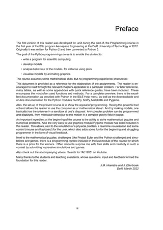


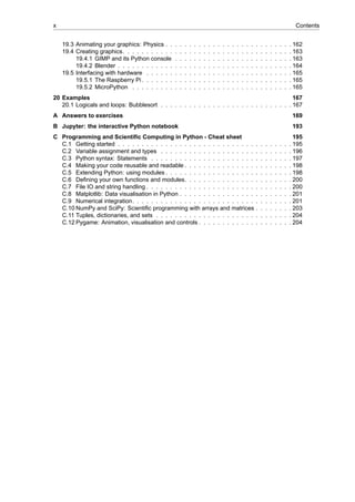
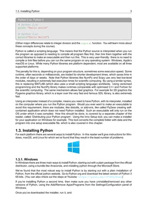
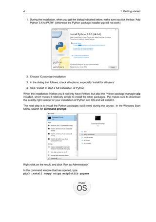
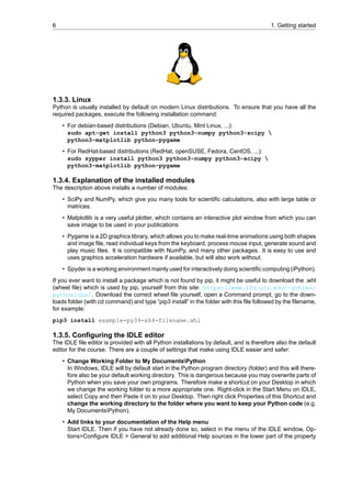
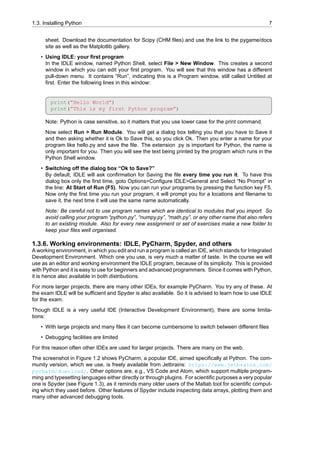
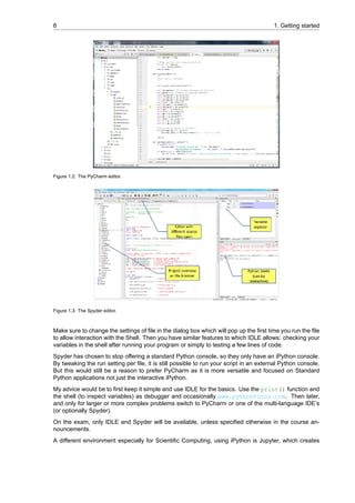
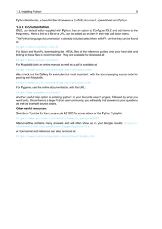
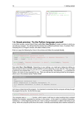
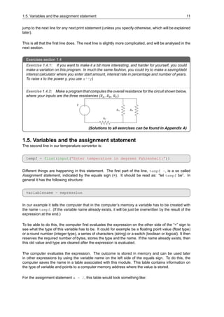
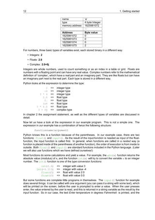
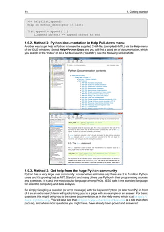
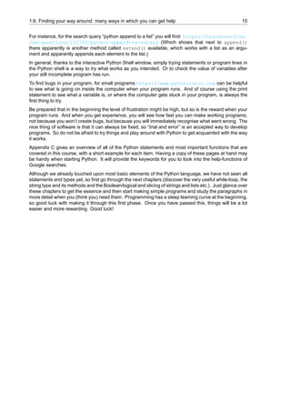

![2.2. Short-hand when using original value with an operator 19
lst = [9 , 2 , 5]
a, b, c = lst
2.2. Short-hand when using original value with an operator
The “=” in an assignment means: “make equal to”. To increase the integer variable i with one, we
normally type:
i = i + 1 # increase i with one
Mathematically speaking this statement would be nonsense if we would read the equal sign as ‘being
equal to’. But as an assignment statement, this simply evaluates the expression on the right side, which
is the content of variable i to which one is added, and the result is stored in the variable i again. The
effect is thus that i is increased with 1. Here are a few other example with the same logic:
j = j - 1 # decrease j with one
n = n * 2 # doubles n
x = x / 2 # halves x
a = a * k # a will be multiplied by k
As especially the increase or decreases with one occurs often, there is a shorthand notation for things:
i = i + => i +=
So the examples above can also be coded like this:
i += 1 # increase i with one
j -= 1 # decrease j with one
n *= 2 # doubles n
x /= 2 # halves x
a *= k # a will be multiplied by k
This short-hand is the same as in the programming language C (and C++), a language which is well
known for how short code can be written (often with an adverse effect on the readability). Also in this
example, the benefit is mainly for the programmer who saves a few keystrokes, (in Python) there is
no execution time benefit as the operations done are the same. This short-hand hence increases the
distance from pseudo-code. Whether you use it is a matter of personal preference.
2.3. Number operations in Python
For the number types float, integer (and complex) the following operators can be used
+ Addition
- Subtraction
* Multiplication
/ Division
// Floored or integer division (rounded off to lower round number)
% Modulo, remainder of division
** Power operator x**y is x to power y, so x**2 is x2
-x Negated value of x
+x Value of x with sign unchanged
As well as the following standard functions:
abs(x) Absolute value of x; |x|
pow(x, y) Power function, same as x ** y
divmod(x, y) Returns both x // y and x % y](https://image.slidesharecdn.com/25527873-250512225116-1392be49/85/Programming-And-Scientific-Computing-In-Python-60-Jm-Hoekstra-33-320.jpg)
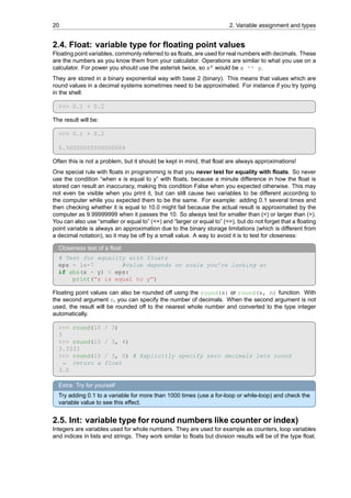
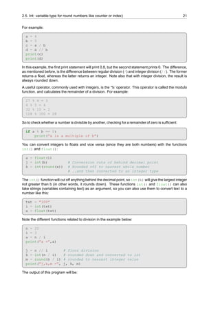
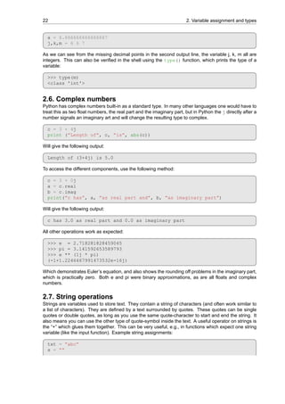
![2.8. Booleans and logical expressions 23
name = ”Graham” + ”Chapman” # (so the + concatenates strings)
words = 'def ghi'
a = input(”Give value at row” + str(i))
Some useful basic functions for strings are:
len(txt) returns the length of a string
str(a) converts an integer or float to a string
eval(str) evaluates the expression in the string and returns the number
chr(i) converts ASCII code i to corresponding character (see table 2.1)
ord(ch) returns ASCII code of the character variable named ch
Using indices in square brackets [ ] allows you to take out parts of a string. This is called slicing. You
cannot change a part of string but you can concatenate substrings to form a new string yielding the
same effect:
c = ”hello world”
c[0] is then ”h” (indices start with zero)
c[1:4] is then ”ell” (so when 4 is end, it means until and not including 4)
c[:4] is then ”hell”
c[4:1:-1] is then ”oll” so from index 4 until 1 with step -1
c[::2] is then ”hlowrd”
c[-1] will return last character ”d”
c[-2] will give one but last character ”l”
c = c[:3] + c[-1] will change c into ”hel” + ”d” = ”held”
The string variable also has many functions built-in, the so-called string methods. See some examples
below (more on this in chapter 8).
a = c.upper() returns copy of the string but then in upper case
a = c.lower() returns copy of the string but then in lower case
a = c.strip() returns copy of the string with leading and trailing spaces removed
sw = c.isalpha() returns True if all characters are alphabetic
sw = c.isdigit() returns True if all characters are digits
i = c.index(”b”) returns index for substring in this case “b”
For more methods see chapter 8, or section 5.6.1 of the Python supplied reference documentation in
the Help file.
Strings are stored as lists of characters. Internally, Characters are stored by the computer as numbers,
using the Unicode encoding. This encoding is an extension of the ASCII codes. See table 2.1:
ASCII codes can be derived from the corresponding character using the ord(char) function. Similarly,
the character for a given ASCII code i can be retrieved using the chr(i) function. As you may
have noticed in table 2.1, the first 31 and the last entry are ‘special’ characters. Most of these special
characters you will likely never need. Exceptions to this are the newline character, and the tab character.
These special can be easily entered into a string using an ‘escape character’: a backslash followed
by a character. In this way, you can add a newline to a string by adding 'n', and a tab by adding
't'. When you start reading text files from disk (see chapter 8), you might notice that newlines can
also be indicated with other characters: In Windows/DOS text files the newline is indicated by both
a Carriage Return and a Line Feed: chr(13) + chr(10). On Linux and Apple systems only the
newline character chr(10) is used.
2.8. Booleans and logical expressions
Booleans (or logicals) are two names for the variable type in which we store conditions. You can see
them as switches inside your program. Conditions can be either True or False, so these are the only
two possible values of a logical. Mind the capitals at the beginning of True and False when you use
these words: Python is case sensitive. Examples of assignments are given below:](https://image.slidesharecdn.com/25527873-250512225116-1392be49/85/Programming-And-Scientific-Computing-In-Python-60-Jm-Hoekstra-37-320.jpg)
![24 2. Variable assignment and types
0 NUL (Null) 32 SP 64 @ 96 ‘
1 SOH (Start of Header) 33 ! 65 A 97 a
2 STX (Start of Text) 34 ” 66 B 98 b
3 ETX (End of Text) 35 # 67 C 99 c
4 EOT (End of Transmission) 36 $ 68 D 100 d
5 ENQ (Enquiry) 37 % 69 E 101 e
6 ACK (Acknowledgement) 38 & 70 F 102 f
7 BEL (Bell) 39 ' 71 G 103 g
8 BS (Backspace) 40 ( 72 H 104 h
9 HT (Horizontal Tab) 41 ) 73 I 105 i
10 LF (Line Feed) 42 * 74 J 106 j
11 VT (Vertical Tab) 43 + 75 K 107 k
12 FF (Form Feed) 44 , 76 L 108 l
13 CR (Carriage Return) 45 - 77 M 109 m
14 SO (Shift Out) 46 . 78 N 110 n
15 SI (Shift In) 47 / 79 O 111 o
16 DLE (Data Link Escape) 48 0 80 P 112 p
17 DC1 (Device Control 1 (XON)) 49 1 81 Q 113 q
18 DC2 (Device Control 2) 50 2 82 R 114 r
19 DC3 (Device Control 3 (XOFF)) 51 3 83 S 115 s
20 DC4 (Device Control 4) 52 4 84 T 116 t
21 NAK (Negative Acknowledgement) 53 5 85 U 117 u
22 SYN (Synchronous Idle) 54 6 86 V 118 v
23 ETB (End of Transmission Block) 55 7 87 W 119 w
24 CAN (Cancel) 56 8 88 X 120 x
25 EM (End of Medium) 57 9 89 Y 121 y
26 SUB (Substitute) 58 : 90 Z 122 z
27 ESC (Escape) 59 ; 91 [ 123 {
28 FS (File Separator) 60 < 92 124 |
29 GS (Group Separator) 61 = 93 ] 125 }
30 RS (Record Separator) 62 > 94 ^ 126 ~
31 US (Unit Separator) 63 ? 95 _ 127 DEL
Table 2.1: The ASCII table.
found = False
prime = True
swlow = a < b
outside = a >= b
swfound = a == b
notfound = a != b # ( != means: not equal to)
outside = x < xmin or x > xmax or y < ymin or y > ymax
inside = not outside
out = outside and (abs(vx) > vmax or abs(vy) > vmax)
inbetween = 6.0 < x <= 10.0
Conditions are a special kind of expression used in statements like if and while to control the flow
of the execution of the program. In the above statements, often brackets are used to indicate that it is
a logical expression.
NB: Testing equality vs assignment
To test whether two variables are the same, you have to use two equals signs (==). This is easily
confused with the assignment statement, which uses a single equals sign (=)! In most cases, when
you confuse these two, your program will still run, but the results will obviously not be what you](https://image.slidesharecdn.com/25527873-250512225116-1392be49/85/Programming-And-Scientific-Computing-In-Python-60-Jm-Hoekstra-38-320.jpg)
![2.9. The list type: an ordered collection of items 25
expect! So remember: Two equals signs will check the condition and one equals sign assigns an
expression to a variable name.
Extra: Alternative syntax for ‘not equal to’
For “is not equal to” both != as well as <> can be used, but != is preferred.
With combined conditions with many “and”, “or” and “not” statements use brackets to avoid confu-
sion:
not((x > xmin and x < xmax) or (y > ymin and y < ymax))
You can use logicals as conditions in if and while statements:
if inside:
print(”(x,y) is inside rectangle”)
while not found:
i = i + 1
found = (a == lst[i])
Note that if inside basically means: if inside == True and similarly while not found
means while found == False. This is why Booleans are never compared with True or False as
this serves no function (for more information on if-statements, see section 3.4, for while-statements,
see section 3.6).
2.9. The list type: an ordered collection of items
2.9.1. What are lists?
Lists are a way to group variables together. This allows you to repeat something for all elements of a list
by using an index as a counter or by iterating through the list with the for-statement (see section 3.5).
This could be a repetitive operation, but also a search or a sorting action. Often it is useful to have a
series of variables that are grouped together. You can therefore look at a list as if it is a table. Each
element of a list can be of any type: it can be an integer, float, logical, string or even a list! Special for
Python is that you can even use different types in one list; in most programming languages this would
not be possible. Both to define a list, as well as to specify an index, square brackets are used as in
strings:
Creating lists
a = [2.3 , 4.5 , -1.0, .005, 2200.]
b = [20, 45, 100, 1, -4, 5]
c = [”Adama”, ”Roslin”, ”Starbuck”, ”Apollo”]
d =[[”Frederik”,152000.0], [”Alexander”,193000.0],
[”Victor”,110000.0]]
e = []
This would make the variable a a list of floats, b a list of integers, and c a list of strings. A list of lists
as defined in d is basically a way to create a two-dimensional list. Finally e is an empty list. Accessing
elements from the list is done as indicated below. Another way to make a list of numbers is using the
so-called range function. This is a so-called iterator function used primarily in loops, but it can also be
converted to a list. The range function can contain one two or even three arguments:
range(stop)
range(start, stop))
range(start, stop, step))](https://image.slidesharecdn.com/25527873-250512225116-1392be49/85/Programming-And-Scientific-Computing-In-Python-60-Jm-Hoekstra-39-320.jpg)
![26 2. Variable assignment and types
In all these cases start is the start value (included), stop is the value for which the block is not
executed because for will stop when this value is reached. So it is an inclusive start but excludes stop.
Another option is to enter a third argument, to indicate a stepsize. The default start is 0, the default
step is 1. Note that range() only works with integers as arguments:
list(range(5)) gives [0, 1, 2, 3, 4]
list(range(5,11)) gives [5, 6, 7, 8, 9, 10]
list(range(5,11,2)) gives [5, 7, 9]
2.9.2. Indexing and slicing, list functions and delete
Let’s use the following list:
lst = [1, 2, 3, 4, 5, 6, 7, 8, 9, 10]
If we now print elements we can use the indices in many ways. Using one index, indicating a single
element:
lst[0] which holds value 1
lst[1] which holds value 2
lst[9] which holds value 10
lst[-1] last element, which holds the value 10
lst[-2] one but last element which holds the value 9
Here it can be seen that indices start at 0, just as with strings. And similar to strings, the function len()
will give the length of a list and thus the not to reach maximum index for the list. Slicing lists with indices
works in the same way as it does for strings, with three possible arguments: start, stop and step. Only
one index refers to one single element. Two arguments separated by a colon refer to start and stop. A
third can be used as step. If you look at the lists that were made in the previous paragraph about lists
you can see that:
a[1] will return a float 4.5
b[1:4] will return a list [45, 100, 1]
d[1][0] will return ”Alexander” (do you see the logic of the order of the in-
dices for the different dimensions: second element of main list, then first
element of that list?)
Adding and removing elements to a list can be done in two ways: the “+” operator, or the append and
extend functions:
a = a + [3300.0] will add 3300.0 at the end of the list
a = a[:-2] will remove the last two elements of the list (by first copying
the complete list without the last two elements, so not very
efficient for large lists)
a = a[:i]+a[i+1:] will remove element i from the list, when it’s not the last one
in the list
a = b + c will concatenate (glue together) two lists if b and c are lists
Another way is to use the del (delete command) and/or functions which are a part of the list class.
You call these functions using the dot notation: variablename.functionname() so a period be-
tween variablename and functionname. Some examples:
a.append(x) add x as a list element at the end of the list named a, equiva-
lent to a = a + [x]
a.extend(b) extend the list with another list b, equivalent to a = a + b
a.remove(3300.0) removes the first element with value 3300.0
del a[-1] removes the last element of a list named a
del a[3:5] removes the 4th till the 6th element of a list named a
a = a[:3] + a[4:] will remove the 4th element of the list named a
Slicing](https://image.slidesharecdn.com/25527873-250512225116-1392be49/85/Programming-And-Scientific-Computing-In-Python-60-Jm-Hoekstra-40-320.jpg)
![2.9. The list type: an ordered collection of items 27
The last example line uses the slicing notation (which can also be used on strings!). Slicing, or cutting
out parts of a list is done with the colon notation. Slicing notation is similar to the range arguments:
start:stop and optionally a step can be added as third argument: start:stop:step. If no value
is entered as start, the default value is zero. If no value is added as end the default value is the last
element. The default step size is 1. Negative values can be used to point to the end (-1 = last element,
-2 is the one-but-last, etc.).
Using the original definition of the lst variable: lst = [1, 2, 3, 4, 5, 6, 7, 8, 9, 10],
this will give:
lst[:3] first three element index 0,1,2: [1,2,3]
lst[:-2] all except last two elements
lst[4:] all elements except the first four: except elements nr 0,1,2,3
lst[::2] every second element so with index 0,2,4, until the end
Other useful functions for lists:
b.index(45) will return the index of the first element with value 45
len(d) will return the length of the list
min(a) will return the smallest element of the list variable a
max(a) will return the largest element of the list variable a
sum(a) will return the sum of the elements in the list variable a
2.9.3. Quick creation of lists with repeating values
If you need to create a one-dimensional list with multiple times the same value, Python offers the
following short-hand:
a = 5 * [0]
print(a) # Would print [0, 0, 0, 0, 0]
a[1] = 1
print(a) # Would print [0, 1, 0, 0, 0]
This notation, however, does not work for nested (two-dimensional) lists. When you need this, you can
use a loop to construct your list:
a=[]
for i in range(3):
a.append(3*[0])
a[0][1] = 1
print(a) # Would print [[0, 1, 0], [0, 0, 0], [0, 0, 0]]
This is a safe way of constructing nested lists, as each new element of a is constructed from scratch.
The following would also work:
# if your list is small, just do it entirely by hand
a = [[0, 0], [0, 0], [0, 0]]
# You can also initialise your list with dummy values, which you replace
afterwards:
↪
a = [0, 0, 0]
for i in range (3):
a[i] = [0, 0]
If you are not sure, test a simple example by constructing your nested list, changing one of its elements,
and see the effect by printing the entire list. You can also use www.pythontutor.com to visualise
what is going on in the computer’s memory. In the above example we use a for-loop to execute a line
of code a fixed (in this case 3) number of times. You’ll learn more about for-loops in section 3.5.](https://image.slidesharecdn.com/25527873-250512225116-1392be49/85/Programming-And-Scientific-Computing-In-Python-60-Jm-Hoekstra-41-320.jpg)
![28 2. Variable assignment and types
Extra: The tricky nature of mutable types
Although the short-hand notation described above doesn’t give you what you’d expect, it doesn’t
return an error either. What happens is the following:
a = 3 * [3 * [0]]
print(a) # Would print [[0, 0, 0], [0, 0, 0], [0, 0, 0]]
a[0][1] = 1
print(a) # Would print [[0, 1, 0], [0, 1, 0], [0, 1, 0]]
The result of the second print statement is probably not what you expected! In line 3 we only
change the second element of the first row, but surprisingly all rows (all lists) have their second
element changed into 1!
What happens is related to the fact that some types are mutable (lit. ‘can be changed’), and others
immutable (lit. ‘cannot be changed’). In Python, all basic types, like floats, integers, and booleans
are immutable. So in the following, variable a is copied into b:
a = 1 # Create an integer variable in memory, with value 1
b = [a, a, a] # Create a list, with three copies of a as content
However, aggregate types (i.e., combinations of multiple data, such as a list) are mutable, which
in Python means that they are passed by reference. This results in the following:
a = [0, 0] # Create a list
b = [a, a, a] # Create a second list, with three references to a as
content
↪
Here, b literally contains three times the original variable a. Changing the contents of a therefore
results in the same behaviour as the short-hand construction of nested lists:
a[0] = 1
print(b) # Would print [[1, 0], [1, 0], [1, 0]]
Have a look at this Python-tutor example for a visualisation of such construction and referencing!
2.9.4. List methods
Another powerful attribute of Python’s list is the number of methods that come with it. Methods are
functions which you call with the dot-notation, as you already saw in section 2.9.2, and in the previous
section with the append() method. An example of this is the sort method:
a = [2, 10, 1, 0, 8, 7]
a.sort()
print(a) # Would print [0, 1, 2, 7, 8, 10]
As we can see the method sort() (you can recognise functions and methods by the presence of
parentheses) sorts the list a. This is a special function in that it changes the actual source list instead
of creating a sorted copy (this is called an in-place operation). Most methods will return the result of
the function as a new variable, and leave the original intact. Examples are the methods index and
count. Index will give the index of the first occurrence of the given value. Count will give the total
number of occurrences:
>>> a = [3,1,8,0,1,7]
>>> a.count(1)
2
>>> a.index(1)
1](https://image.slidesharecdn.com/25527873-250512225116-1392be49/85/Programming-And-Scientific-Computing-In-Python-60-Jm-Hoekstra-42-320.jpg)
![2.10. Some useful built-in functions 29
>>> a.index(9)
Traceback (most recent call last):
File ”<pyshell#23>”, line 1
a.index(9)
ValueError: 9 is not in list
>>>
How would you make a program which will print the index of the first occurrence but also avoids the
error message if it is not found by simply printing -1?
Exercises section 2.9
Exercise 2.9.1: Make a program which calculates effect of a yearly interest rate (entered by the
user) on start sum (also entered by the user). Print the amount after each year (ask the user how
many years).
Exercise 2.9.2: Make a list of words input by the user (e.g. aeroplane company names) by using
the append() function, then print them below each other with the length of each word.
Exercise 2.9.3: You can also make a list which consists of different lists, each with a different
length, as shown here:
values = [[10, 20], [30, 40, 50, 60, 70]]
Print the length of each list and all the values it contains.
Exercise 2.9.4: We can also go in the other direction, and construct a list of lists from a list of
values and a list of lengths:
values = [10, 20, 30, 40, 50, 60, 70] lengths = [2, 2, 3]
Construct a list of lists, with each list i containing lengths[i] values from values. Print the
constructed list.
2.10. Some useful built-in functions
As we have already seen in the examples, Python has a number of built-in functions which you can
use in the right side of assignment statements on any expression using values and variables:
float(i) converts an integer or string(text) to a float
int(x) converts a float to an integer (whole number rounded to
lowest integer)
round(x) rounds off to nearest round number and converts to in-
teger
round(x,n) rounds off a float n decimals, result is still float
str(x) converts a number into a string (text)
eval(txt) converts a text to a number
bool(x) convert x to a Boolean (typically non zero is True)
repr(x) generates a string with a printable content of x
list(txt) converts x to a list type (e.g. splits string in single char-
acters)
chr(i) gives character for ascii code i (look up ascii table to see
codes)
ord(c) gives acsii code of character c (a string with length one)
len(txt) gives length of the string txt
len(lst) gives length of the list lst
abs(x) absolute value of x (modulo/length for complex numbers)
range(stop) give a list [0,1,...stop-1] so stop is not included](https://image.slidesharecdn.com/25527873-250512225116-1392be49/85/Programming-And-Scientific-Computing-In-Python-60-Jm-Hoekstra-43-320.jpg)
![30 2. Variable assignment and types
range(start,stop) give a list [start, start+1,...,stop-1] so start is included!
range(start,stop,step) give a list [start, start+step,...] stop is not included
sum(a,b,c,d,...) total sum of variables a,b,c,d,...
sum(lst) total sum of the list elements in lst
max(a,b,c,d,...) maximum value of a,b,c,d,...
max(lst) maximum value in the list lst
min(a,b,c,d,...) minimum value of a,b,c,d,...
min(lst) minimum value in the list lst
input(txt) prints txt, asks user for input, returns user input as a text
string
help(txt) for use in shell: prints help on Python or installed
function, module or statement, e.g. help(’math’) or
help(’input’)](https://image.slidesharecdn.com/25527873-250512225116-1392be49/85/Programming-And-Scientific-Computing-In-Python-60-Jm-Hoekstra-44-320.jpg)
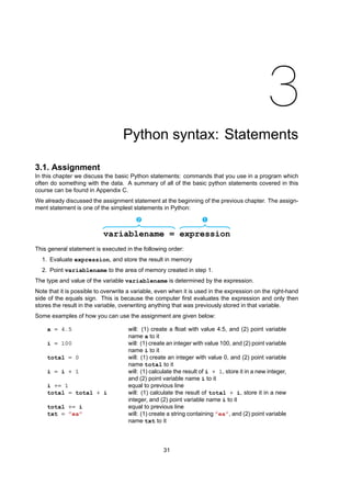
![32 3. Python syntax: Statements
txt = txt + ”sy” will: (1) evaluate the expression txt + ”sy”, store the result
(”easy”) in a new string, and (2) point variable name txt to
it
series = [] will: (1) create an empty list, and (2) point variable name se-
ries to it
series = series + [i] will: (1) create a new list, containing the contents of series,
appended with an additional element i, and (2) point variable
name series to it
Here it should be noted that a statement such as i = i + 1 may seem mathematically incorrect,
but in programming this simply means that the expression i + 1 is evaluated with the old value of
i, after which the variable i is updated to point to the result of the expression. This order of actions
basically means that ‘=’ means ‘will become’ instead of ‘is equal to’ (remember that for the ‘is equal
to’ comparison ‘==’ in Python). Also note the short-hand notation “+=”, which has been discussed
extensively in section 2.1 already.
Adapting our example program from the previous chapter, we add some logic. Edit the program to
match this example precisely, note the margin jumps (use TAB-key) in the if statement, which is
called indentation. Having the same margin, or indentation level, is what Python uses to mark blocks
of code that belong together, for example because they are part of an if-branch or a loop (see later
sections on for and while loops).
ABC solver with discriminant check
from math import sqrt
print(”To solve ax2 + bx + c = 0 :”)
a = float(input(”Enter the value of a: ”))
b = float(input(”Enter the value of b: ”))
c = float(input(”Enter the value of c: ”))
D = b ** 2 - 4.0 * a * c
if D < 0.0:
print(”This equation has no solutions”)
else:
x1 = (-b - sqrt(D)) / (2.0 * a)
x2 = (-b + sqrt(D)) / (2.0 * a)
print(”x1 =”, x1)
print(”x2 =”, x2)
Now the program first checks whether D is negative. If so, it will tell you that there are no solu-
tions.
• Note the structure and syntax(=grammar) of the if-else statement. A colon ( : ) indicates that
a block of code will be given, so it acts as a ‘then’. The block is marked by the increased level of
indentation of the code.
• When it jumps back to the margin of the beginning to indicate the end of this block of code, an
‘else’ follows, again with a colon and an indented block of code.
• It also uses a different way to import the sqrt function from the math module. Note the dif-
ference in syntax in both the line with the import statement as well as the line where the sqrt
function is used. Chapter 5 will explain the different ways to import modules.](https://image.slidesharecdn.com/25527873-250512225116-1392be49/85/Programming-And-Scientific-Computing-In-Python-60-Jm-Hoekstra-46-320.jpg)
![3.2. The print statement 33
Exercises section 3.1
Exercise 3.1.1: Adapt the program so that it calculates the hypotenuse c of a rectangular triangle
for rectangular sides a and b as entered by the user, using Pythagoras formula.
Exercise 3.1.2: Using the flow chart depicted below, make a program that determines the
maximum value of given numbers a, b, c and d as entered by the user, using a number of if-
else-statements to find the maximum value of these four variables.
start
Enter values
a, b, c, d
a > b?
max1 = a max1 = b
c > d?
max2 = c max2 = d
max1 > max2?
end
print max1 print max2
Exercise 3.1.3: Write a program that clamps a float input by the user to [-10, 10] and prints it.
Additionally, if the input is negative, the program should print a warning message.
3.2. The print statement
The print function generates text output in the console. It can print text, variables and (the result
of) expressions. To print several things on one line, pass them to the print function, separated by
commas. In the resulting printed line of text, a space will automatically be inserted between each
argument. The space is the default so-called ‘separator’ symbol. After each call to print automatically
a newline character is printed, so the next print call will start at a new line. A print-statement without
any arguments, prints an empty line, or a newline character to be exact.
3.2.1. Using print
Below is an example of four different ways of using the print command, which will result in exactly
the same output (printing the text ‘Hello world’ to the console, followed by a newline):
# Method 1
print(”Hello world”)
# Method 2
print(”Hello”, ”world”, sep=” ”)
# Method 3](https://image.slidesharecdn.com/25527873-250512225116-1392be49/85/Programming-And-Scientific-Computing-In-Python-60-Jm-Hoekstra-47-320.jpg)
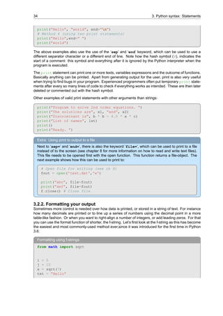
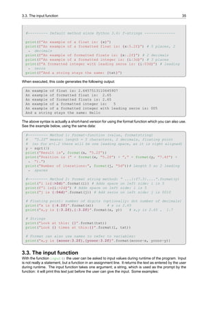
![36 3. Python syntax: Statements
Using the input function to get data from the user
name = input(” What is your name: ”)
ans = input(” Do you want to continue? (Y/N) ”)
The input function will always return a string. When another type of variable is needed as input, the
converter functions can be used to get the right type:
x = float(input(”Give value for x: ”))
i = int(input(”Give number of values: ”))
In some cases this might not work, for instance when we want to enter an expression (maybe even
using variable names). It will also not work when a list of values is entered by the user. In both cases
successful conversion can be achieved by using an alternative method, the evaluation function eval()
can be used for the conversion of the string. A call to eval() will evaluate any expression as an actual
Python expression, and determine the type in the same as the assignment function would do it:
The eval function
xlst = list(eval(input(”Give values for x: ”)))
a, b, c = eval(input(”Enter a,b,c: ”))
The eval function could also be used in the examples above, but there is a risk of the type ending up
different from what you expected. Users will not always add a decimal point when entering a float for
instance.
Note the difference between print and input, in terms of the arguments they accept. While print
takes any number of arguments, which it combines together in a single printed output, separated by
spaces, input only takes one argument. There are different ways to get around this. The first is to
use print in combination with input:
print(”Enter the value of coordinate”, i, ”:”, end=” ”)
x[i] = input()
Another approach would be to generate a single string of text before passing it to input:
# Join strings together with +
x[i] = input(”Enter the value of coordinate” + str(i) + ”: ”)
# Or create a combined string using f-strings
x[i] = input(f”Enter the value of coordinate {i} : ”)
The second option in the box above uses f-strings, see the previous section on formatting your print
output. This method is even more powerful than joining strings with the ‘+’ operator.
3.4. Checking conditions: the if-statement
Almost any program relies at some point on the ability to test a certain condition: have we reached the
end of a list?, has our simulated Mars lander hit the ground? and so on. Such condition checking is
done using the if-statement. This statement has the following syntax:
Ê Ë
if condition:
Ì
# Execute only when condition is true
statements
Here, the elements are:
1. The statement keyword if](https://image.slidesharecdn.com/25527873-250512225116-1392be49/85/Programming-And-Scientific-Computing-In-Python-60-Jm-Hoekstra-50-320.jpg)
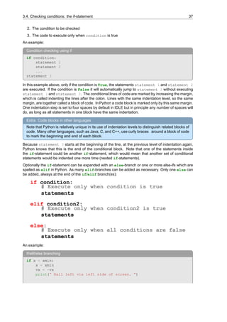
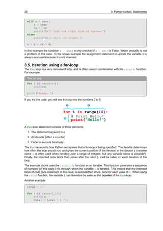
![3.5. Iteration using a for-loop 39
print(total)
In this example, a variable total is initialised as zero just before the loop. Then, in every iteration of
the loop i * i is added to total. Since i runs from 1 until but, not including, 11 in this code, the result
is that total will be equal to 1*1 + 2*2 +3*3+ ... + 9*9 + 10*10.
Instead of using range() to generate a range of integers, you can also use a for-loop to iterate
directly over the contents of a list:
Iterating directly over a list
fellowship = [”Frodo”, ”Sam”, ”Merry”, ”Pippin”, ”Gandalf”,
”Legolas”, ”Gimli”, ”Aragorn”, ”Boromir”]
for name in fellowship:
print(name)
If you need to iterate over a range of floats, e.g., from 0.0 to 10.0, with a step of 0.1, you can also use
the following construction. This example will print these values:
for i in range(101):
x = i * 0.1
print(x)
Tip: When setting up loops (while or for), use print statements first (e.g. with a small number of
iterations) to see whether your loop does what you intend it to do.
3.5.1. Additional tools for for-loops: itertools
The module itertools has a lot of iteration tools which are very useful in combination with a for-
loop. It for instance provides functions to get any permutation or combination of elements in a loop. This
can save a lot of programming time compared to when you would have to make that yourself.
For example, this bit of code uses the permutations iterator function, which takes a list as input:
Using itertools’ permutations
from itertools import permutations
lst = [1, 2, 3]
for a in permutations(lst):
print (a, end=” ”)
When executed, this code will generate the following output:
(1, 2, 3) (1, 3, 2) (2, 1, 3) (2, 3, 1) (3, 1, 2) (3, 2, 1)
The combinations(lst, n) function can be used to generate all n-sized combinations from the
values provided in lst:
from itertools import combinations
lst = [1, 2, 3, 4, 5]
for a in combinations(lst, 2):
print (a, end=” ”)
When run, this code will print:](https://image.slidesharecdn.com/25527873-250512225116-1392be49/85/Programming-And-Scientific-Computing-In-Python-60-Jm-Hoekstra-53-320.jpg)
![40 3. Python syntax: Statements
(1, 2) (1, 3) (1, 4) (1, 5) (2, 3) (2, 4) (2, 5) (3, 4) (3, 5) (4, 5)
There are many more useful functions in itertools, such as cycle, product, etc. In the python shell,
type help(”itertools”) to see a complete overview.
Exercises section 3.5
Exercise 3.5.1: Make a program that prints all the prime numbers until a certain value, (recall
that a prime number is not divisible by any number except itself and 1).
Exercise 3.5.2: Write a Python program to construct the pattern shown below:
*
* *
* * *
* * * *
* * * * *
* * * *
* * *
* *
*
Exercise 3.5.3: Write a Python program that accepts a string and counts the number of digits
and letters in the string.
3.6. Iteration using a while-loop
A more versatile loop is the while-loop. It is a sort of a combination between an if-statement and
a for-loop. A block of statements is executed for as long as a given condition is True. The block is
repeated until the condition becomes False. The syntax of such a while-loop is:
Syntax of the while loop
while condition:
statement 1
statement 2
statement 3
Because it evaluates a condition, while is just like if: it is used to control the flow of a program
based on a condition. The difference with if is that the condition checking in the case of while is
automatically repeated, until the condition becomes False.
Below is an example of a while-loop:
h0 = [0.0, 11000.0, 20000.0, 32000.0, 47000.0, 51000.0, 71000.0]
hmax = h0[-1]
h = float(input(”Enter altitude”))
h = min(h, hmax)
i = 0
while h > h0[i + 1]:
i = i + 1
When you use this as a sort of “repeat until”, you have to prepare the condition which is tested by
while in such a way that the first time it will be True, so the loop is entered at least once. You can see
this in the second example below, where found is set to False first.
Another example:](https://image.slidesharecdn.com/25527873-250512225116-1392be49/85/Programming-And-Scientific-Computing-In-Python-60-Jm-Hoekstra-54-320.jpg)