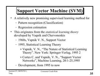
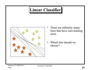
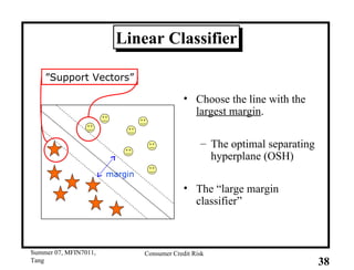
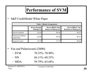
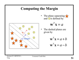
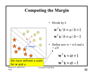
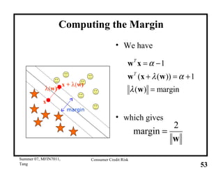
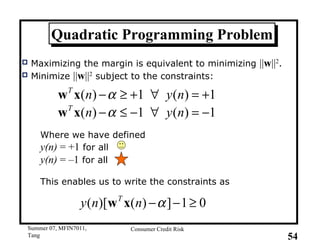
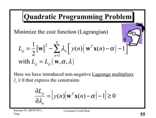
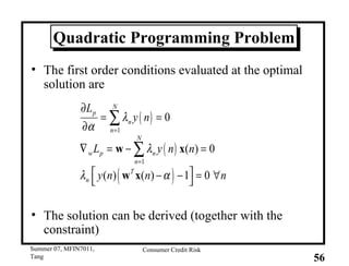
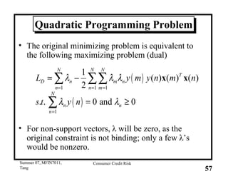
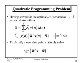
MFIN 7011: Credit Risk Management Summer, 2007 Dragon Tang Lecture 18 Consumer Credit Risk Thursday, August 2, 2007 Readings:  Niu (2004); Agarwal, Chomsisengphet, Liu, and Souleles (2006)
Consumer Credit Risk Objectives : Credit scoring approach for consumer credit risk Practice, challenge, and opportunity
Consumer Credit Default Risk (low in general) Low High Credit Products Fixed Term Revolving Residential Mortgage Retail Finance Personal Loans Overdrafts Credit Cards
Consumer Lending Examples: Automobile loans Home equity loans Revolving credit  There is an exponential growth in consumer credit outstanding in the US, from USD 9.8 billion in 1946 to USD 2411 billion in  January 2007 $878 billion revolving; $1526 billion non-revolving Currently interest rate is 13%; interest accessed is 15%
Consumer vs. Corporate Lending Consumer lending is not as glamorous as corporate lending Consumer lending is a volume business, where low cost producers who can manage the credit losses are able to enjoy profitable margins Corporate lending is often unprofitable as every bank is chasing the same corporate customers, depressing margins
Consumer Credit Risk: Art or Science? Art:  consumers care about reputation Value of reputation is hard to model Reduced form model may be useful Science:  creditworthiness can be predicted from financial health Using structural models of Merton type The answer is probably both! Hybrid structural-reduced form model should be most promising
Never make predictions, especially about the future. — Casey Stengel
The credit Decision Scoring vs. Judgmental Both methods Assume that the future will resemble  the past Compare applicants to past experience Aim to grant credit only to acceptable risks Added value of scoring Defines degree of credit risk for each applicant Ranks risk relative to other applicants Allows decisions based on degree of risk Enables tracking of performance over time Permits known and measurable adjustments Permits decision automation
Evaluating the credit applicant Time at present address Time at present job Residential status Debt ratio Bank reference Age Income # of Recent inquiries % of Balance to avail. lines # of Major derogs. Overall Decision Odds of repayment • • • CHARACTERISTICS + + - + + N / A - - + + + Accept ? • • • JUDGMENT 12 20 5 21 28 15 5 -7 10 35 212 Accept 11:1 • • • CREDIT SCORING
Credit Scoring Project Input x feature vector Label y, default or not Data (x i  , y i ) Target y=f(x) Objective Given new x, predict y so that probability of error is minimal
Typical Input Data Time at present address  0-1, 1-2, 3-4, 5+ years Home status  Owner, tenant, other Telephone  Yes, no Applicant's annual income  $(0-10000),  $(11000-20000), $(21000+) Credit card  Yes, no Type of bank account  Cheque and/or savings, none Age  18-25, 26-40, 41-55, 55+ years Type of occupation  Coded Purpose of loan  Coded Marital status  Married, divorced, single, widow Time with bank  Years Time with employer  Years
Input Data: FICO Score Not in the score: demographic data
Characteristics of Data X: Continuous Discrete  Normal distribution? Y: Binary data: 0 or 1 (=default)
Scoring Models Statistical Methods DA (Discriminant Analysis) Linear regression Logistic regression Probit analysis Non-parametric models Nearest-neighbor approach
Statistical Methods:  Discriminant Analysis Multivariate statistical analysis: several predictors (independent variables) and several groups (categorical dependent variable, e.g. 0 and 1) Predictive DA: for a new observation, calculate the discriminant score, then classify it according to the score The objective is to maximize the between group to within group sum of squares ratio that results in the best discrimination between the groups (within group variance is solely due to randomness; between group variability is due to the difference of the means) Normal distribution for the response variables (dependent variables) is assumed (but normality only becomes important if significance tests are to be taken for small samples)
Statistical Credit Scoring Credit Score #Customers Good Credit Bad Credit Cut-off Score
Statistical Credit Scoring Credit scoring systems: Altman Z-score model: Z = .012 X 1 +.014 X 2 +.033   X 3  +.006   X 4  +1.0 X 5 X 1  = working capital/total assets ratio X 2  = retained earnings/total assets ratio X 3  = earnings before interest and taxes/total assets ratio X 4  = market value of equity/book value of total liabilities ratio X 5  = sales/total assets ratio
Statistical Methods:   Linear Regression The regression model is like: For the true model, u can take only two values as Y; thus u can’t be normally distributed. u has heteroskedastic variances, which makes the OLS inefficient The estimated probability may well lie outside [0,1].
Statistical Methods: Nearest-Neighbor Approach A historical database has been divided into two groups (good and bad) When a consumer comes, calculate the distance between the consumer and everyone in the database The consumer will be classified in the category which is the same as the nearest one(s) Problems: The definition of distance and the number of the nearest ones Scoring speed: when a new x comes, we need calculate the distance between the new x and all of the historical data; too much calculation!
Scoring Models Non-statistical Methods Mathematical programming Recursive partitioning Expert systems Machine Learning Neural Networks Support Vector Machine (SVM)
Which Method is Best? In general there is no overall best method. What is best will depend on the details of the problem: The data structure The characteristics used  The extent to which it is possible to separate the classes by using those characteristics The objective of the classification (overall misclassification rate, cost-weighted misclassification rate, bad risk rate among those accepted, some measure of profitability, etc.)  In the following slides, we will introduce three models, Logistic, Neural Networks, and SVM in detail, which are used widely today
Logistic Regression Empirical studies show, logistic regression may perform better than linear models (Hence, better than Discriminant Analysis), when data is nonnormal (particularly for binary data), or when covariance matrices of the two groups are not identical.  Therefore, logistic regression is the   preferred   method among the statistical methods Probit regression is similar to logistic regression
Performing Logistic Regression Logistic Regression can be performed  using the Maximum Likelihood method In the maximum likelihood method, we are seeking parameter values that maximize the likelihood of the observations occurring
Logistic Regression: Setup Directly models the default probability as a function of the input variables X (a vector) Define  Assume
Logistic Regression: Setup Assume the observations are independent, the probability (likelihood) of the observed sample is given by
Logistic Regression and ML ML estimator (of the coefficients a’s) for Logistic Regression can be found by applying non-linear optimization on the above likelihood function. The simplified version is given by
Logistic Regression and ML It is easy to show that the log of the  odds  (= logit) are a linear function: Therefore, the odds  per se  are a multiplicative function.  Since probability takes on values between (0,1), the odds take on values between (0,∞), logits take on values between (-∞,∞). So, it looks very much like linear regression, and it does not need to restrict the dependent variable to values of {0, 1}.  It is not solvable using OLS.
Logistic Function and Distribution
Normal Distribution The tails are much thinner than Logistic
RiskCalc: Moody’s Default Model Probit  Regression Where x is the vector of the ratios
Neural Networks Non-parametric method Non-linear model estimation technique: e.g. Saturation effect: i.e. marginal effect of a financial ratio may decline quickly Multiplicative factors: highly leveraged firms have a harder time borrowing money Neural networks  decide how to combine and transform the raw characteristics in the data, as well as yielding estimates of the parameters of the decision surface Well suited to situations where we have a poor understanding of the data structure
Neural Networks Use the logistic function as the activation function in all the nodes Works well with classification problems Drawbacks May take much longer to train In credit scoring, there is solid understanding of data
Multilayer Perceptron (MLP) The input values X are sent along with 1 to the hidden layer neuron The hidden layer generates a weight and generates a nonlinear output that is sent to the next layer The output neuron takes 1 with input from the hidden layer and generates the output signal When learning occurs, the weights are adjusted so that the final OUTs produce the least error (The output of a single neuron is called OUT) X1 X2 1 H1 H2 1 O Input Layer Hidden Layer Output Layer w01 w12 w21 w22 w11 w02 w1 w2 w0
Multilayer Perceptron (MLP) Input nodes do not perform processing Each hidden and output node processes the signals by an activation function. The most frequently used is given on the right. The parameters, w, are obtained by “training” the Neural Net to historical data.
Support Vector Machine (SVM) A relatively new promising supervised learning method for Pattern recognition (Classification)  Regression estimation This originates from the  statistical learning theory  developed by Vaqnik and Chervonenkis 1960s, Vapnik V. N., Support Vector 1995, Statistical Learning Theory Vapnik, V. N., “The Nature of Statistical Learning Theory”. New York: Springer-Verlag, 1995 2 Cortes C. and Vapnik, V. N., “Support Vector Networks”, Machine Learning, 20:1-25,1995 Development, from 1995 to now
SVM Extension Proximal Support Vector Machine (PSVM) Glenn Fung and Olvi L. Mangasariany 2001 Incremental and Decremental Support Vector Machine Learning  Least Squares Support Vector Machine (LS-SVM) Also, SVMs can be seen as a new training method for learning machines (such as NNs)
Linear Classifier There are infinitely many lines that have zero training error. Which line should we  choose?
Choose the line with the  largest margin . The optimal separating hyperplane (OSH) The “large margin classifier” Linear Classifier margin ” Support Vectors”
Performance of SVM S&P CreditModel White Paper Fan and Palaniswami (2000): SVM  70.35%–70.90% NN 66.11%–68.33% MDA 59.79%–63.68%
Credit Scoring and Beyond Data collected at application will become outdated pretty fast The way a customer uses its credit account is an indicator for future performance (Behavior Scoring) This leads to an update path of PD and credit control tools The future is moving into profitability scoring. Banks should not only care about getting its money back Banks want to extend credit to those it can make a positive NPV, risk-adjusted
Best Practice in Consumer Credit Risk Management Credit decision-making Adopt to changes in economy or within customer segment Credit scoring Adaptive algorithms using credit bureau data and firm’s own experience  Loss forecasting Historical delinquency rates and charge-off trend analysis Delinquency flow and segmented vintage analysis Portfolio management Risk adjusted return on capital (RAROC)
Analytical Techniques Response analysis:  avoid adverse selection consequences that result in increased concentrations of high-risk borrowers Pricing strategies:  avoid “follow the competition”, focus on segment profitability and cash flow Loan amount determination:  avoid to be judgmental, quantify probabilities of losses Credit loss forecasting:  decompositional roll rate modeling, trend and seasonal indexing, and vintage curve Portfolio management strategies:  important for repricing and retention, don’t be judgmental, integrating behavioral element and cash flow profitability analysis ( underwriting ) Collection strategies:  behavioral models are useful
Credit Scoring and Loss Forecasting Two critical components of consumer credit risk analysis Corresponds to default probabilities and loss given default These two are linked Loss given default is higher when default probability is greater Market and economic variables matter In bad economic states, there will be more default and lower recovery Good modeling should achieve stability
Do Consumers Choose the Right Credit Contracts? Agarwal, Chomsisengphet, Liu, and Souleles (2006): Some don’t, especially when the stake is small But consumers with high balance do! Other issues: Personal bankruptcy in the U.S. soared! Avoid/fight predatory lending! (e.g., subprime lending) China is starting to have a consumer credit market
China’s Consumer Spending 64% 9198  8407  7811  7037  6462  6001  5603  TOTAL 80% 441  400  367  330  296  268  244  Services 120% 931  842  752  663  599  507  424  Housing 113% 1170  1057  945  837  739  643  550  Education&Entertainment 112% 614  554  498  437  385  337  290  Transport&Communication 91% 790  727  657  595  569  485  414  Household Durables 22% 958  885  866  791  728  750  785  Clothing 138% 506  455  401  356  300  255  213  Medicine&Healthcare 41% 3789  3487  3326  3029  2845  2756  2684  Food 97-03 2003 2002 2001 2000 1999 1998 1997 %Chg
China’s Consumer Credit Market 1999-2004: Growth rate 52% Automobile loans: 110% Only 15% of auto sales, compared to 80% in U.S. Bankcard: 36% Mostly debit cards Mortgage: 1000% Still a long way to go! Only 8% of GDP, compared to 45% in developed economies Other markets Student loan Credit cards! More opportunities are waiting!
6
Summary Introduction to Consumer Credit Risk: Credit scoring methods Practical issues Exam: Saturday, August 4, 2PM
Review for Exam Topics: Credit risk modeling: structural/reduced-form/incomplete information Recovery rate & default correlation Credit derivatives Credit VaR/Basel II/consumer credit risk Question Types (tentative!): True or False (20%) Multiple Choice (20%) Short Answers (20%) Problems (40%) 60% conceptual; 40% analytical Formulas will be provided if needed.
SVM Approach Details
The plane separating  and  is defined by The dashed planes are given by Computing the Margin margin w
Divide by  b Define new w = w/ b  and   α  = a/b Computing the Margin margin w We have defined a scale for  w  and  a
We have which gives Computing the Margin margin  w) x x +   w)
Quadratic Programming Problem Maximizing the margin is equivalent to minimizing  || w || 2 . Minimize  || w || 2  subject to the constraints: Where we have defined y(n)  = +1  for all  y(n)  = –1  for all This enables us to write the constraints as
Quadratic Programming Problem Minimize the cost function (Lagrangian) Here we have introduced non-negative  Lagrange multipliers   l n     0 that express the constraints
Quadratic Programming Problem The first order conditions evaluated at the optimal solution are  The solution can be derived (together with the constraint)
Quadratic Programming Problem The original minimizing problem is equivalent to the following maximizing problem (dual) For non-support vectors,  λ  will be zero, as the original constraint is not binding; only a few  λ ’s would be nonzero.
Quadratic Programming Problem Having solved for the optimal  λ ’s (denoted as  ), we can derive others  To classify a new data point x, simply solve

Summer 07-mfin7011-tang1922

  • 1.
    MFIN 7011: CreditRisk Management Summer, 2007 Dragon Tang Lecture 18 Consumer Credit Risk Thursday, August 2, 2007 Readings: Niu (2004); Agarwal, Chomsisengphet, Liu, and Souleles (2006)
  • 2.
    Consumer Credit RiskObjectives : Credit scoring approach for consumer credit risk Practice, challenge, and opportunity
  • 3.
    Consumer Credit DefaultRisk (low in general) Low High Credit Products Fixed Term Revolving Residential Mortgage Retail Finance Personal Loans Overdrafts Credit Cards
  • 4.
    Consumer Lending Examples:Automobile loans Home equity loans Revolving credit There is an exponential growth in consumer credit outstanding in the US, from USD 9.8 billion in 1946 to USD 2411 billion in January 2007 $878 billion revolving; $1526 billion non-revolving Currently interest rate is 13%; interest accessed is 15%
  • 5.
    Consumer vs. CorporateLending Consumer lending is not as glamorous as corporate lending Consumer lending is a volume business, where low cost producers who can manage the credit losses are able to enjoy profitable margins Corporate lending is often unprofitable as every bank is chasing the same corporate customers, depressing margins
  • 6.
    Consumer Credit Risk:Art or Science? Art: consumers care about reputation Value of reputation is hard to model Reduced form model may be useful Science: creditworthiness can be predicted from financial health Using structural models of Merton type The answer is probably both! Hybrid structural-reduced form model should be most promising
  • 7.
    Never make predictions,especially about the future. — Casey Stengel
  • 8.
    The credit DecisionScoring vs. Judgmental Both methods Assume that the future will resemble the past Compare applicants to past experience Aim to grant credit only to acceptable risks Added value of scoring Defines degree of credit risk for each applicant Ranks risk relative to other applicants Allows decisions based on degree of risk Enables tracking of performance over time Permits known and measurable adjustments Permits decision automation
  • 9.
    Evaluating the creditapplicant Time at present address Time at present job Residential status Debt ratio Bank reference Age Income # of Recent inquiries % of Balance to avail. lines # of Major derogs. Overall Decision Odds of repayment • • • CHARACTERISTICS + + - + + N / A - - + + + Accept ? • • • JUDGMENT 12 20 5 21 28 15 5 -7 10 35 212 Accept 11:1 • • • CREDIT SCORING
  • 10.
    Credit Scoring ProjectInput x feature vector Label y, default or not Data (x i , y i ) Target y=f(x) Objective Given new x, predict y so that probability of error is minimal
  • 11.
    Typical Input DataTime at present address 0-1, 1-2, 3-4, 5+ years Home status Owner, tenant, other Telephone Yes, no Applicant's annual income $(0-10000), $(11000-20000), $(21000+) Credit card Yes, no Type of bank account Cheque and/or savings, none Age 18-25, 26-40, 41-55, 55+ years Type of occupation Coded Purpose of loan Coded Marital status Married, divorced, single, widow Time with bank Years Time with employer Years
  • 12.
    Input Data: FICOScore Not in the score: demographic data
  • 13.
    Characteristics of DataX: Continuous Discrete Normal distribution? Y: Binary data: 0 or 1 (=default)
  • 14.
    Scoring Models StatisticalMethods DA (Discriminant Analysis) Linear regression Logistic regression Probit analysis Non-parametric models Nearest-neighbor approach
  • 15.
    Statistical Methods: Discriminant Analysis Multivariate statistical analysis: several predictors (independent variables) and several groups (categorical dependent variable, e.g. 0 and 1) Predictive DA: for a new observation, calculate the discriminant score, then classify it according to the score The objective is to maximize the between group to within group sum of squares ratio that results in the best discrimination between the groups (within group variance is solely due to randomness; between group variability is due to the difference of the means) Normal distribution for the response variables (dependent variables) is assumed (but normality only becomes important if significance tests are to be taken for small samples)
  • 16.
    Statistical Credit ScoringCredit Score #Customers Good Credit Bad Credit Cut-off Score
  • 17.
    Statistical Credit ScoringCredit scoring systems: Altman Z-score model: Z = .012 X 1 +.014 X 2 +.033 X 3 +.006 X 4 +1.0 X 5 X 1 = working capital/total assets ratio X 2 = retained earnings/total assets ratio X 3 = earnings before interest and taxes/total assets ratio X 4 = market value of equity/book value of total liabilities ratio X 5 = sales/total assets ratio
  • 18.
    Statistical Methods: Linear Regression The regression model is like: For the true model, u can take only two values as Y; thus u can’t be normally distributed. u has heteroskedastic variances, which makes the OLS inefficient The estimated probability may well lie outside [0,1].
  • 19.
    Statistical Methods: Nearest-NeighborApproach A historical database has been divided into two groups (good and bad) When a consumer comes, calculate the distance between the consumer and everyone in the database The consumer will be classified in the category which is the same as the nearest one(s) Problems: The definition of distance and the number of the nearest ones Scoring speed: when a new x comes, we need calculate the distance between the new x and all of the historical data; too much calculation!
  • 20.
    Scoring Models Non-statisticalMethods Mathematical programming Recursive partitioning Expert systems Machine Learning Neural Networks Support Vector Machine (SVM)
  • 21.
    Which Method isBest? In general there is no overall best method. What is best will depend on the details of the problem: The data structure The characteristics used The extent to which it is possible to separate the classes by using those characteristics The objective of the classification (overall misclassification rate, cost-weighted misclassification rate, bad risk rate among those accepted, some measure of profitability, etc.) In the following slides, we will introduce three models, Logistic, Neural Networks, and SVM in detail, which are used widely today
  • 22.
    Logistic Regression Empiricalstudies show, logistic regression may perform better than linear models (Hence, better than Discriminant Analysis), when data is nonnormal (particularly for binary data), or when covariance matrices of the two groups are not identical. Therefore, logistic regression is the preferred method among the statistical methods Probit regression is similar to logistic regression
  • 23.
    Performing Logistic RegressionLogistic Regression can be performed using the Maximum Likelihood method In the maximum likelihood method, we are seeking parameter values that maximize the likelihood of the observations occurring
  • 24.
    Logistic Regression: SetupDirectly models the default probability as a function of the input variables X (a vector) Define Assume
  • 25.
    Logistic Regression: SetupAssume the observations are independent, the probability (likelihood) of the observed sample is given by
  • 26.
    Logistic Regression andML ML estimator (of the coefficients a’s) for Logistic Regression can be found by applying non-linear optimization on the above likelihood function. The simplified version is given by
  • 27.
    Logistic Regression andML It is easy to show that the log of the odds (= logit) are a linear function: Therefore, the odds per se are a multiplicative function. Since probability takes on values between (0,1), the odds take on values between (0,∞), logits take on values between (-∞,∞). So, it looks very much like linear regression, and it does not need to restrict the dependent variable to values of {0, 1}. It is not solvable using OLS.
  • 28.
  • 29.
    Normal Distribution Thetails are much thinner than Logistic
  • 30.
    RiskCalc: Moody’s DefaultModel Probit Regression Where x is the vector of the ratios
  • 31.
    Neural Networks Non-parametricmethod Non-linear model estimation technique: e.g. Saturation effect: i.e. marginal effect of a financial ratio may decline quickly Multiplicative factors: highly leveraged firms have a harder time borrowing money Neural networks decide how to combine and transform the raw characteristics in the data, as well as yielding estimates of the parameters of the decision surface Well suited to situations where we have a poor understanding of the data structure
  • 32.
    Neural Networks Usethe logistic function as the activation function in all the nodes Works well with classification problems Drawbacks May take much longer to train In credit scoring, there is solid understanding of data
  • 33.
    Multilayer Perceptron (MLP)The input values X are sent along with 1 to the hidden layer neuron The hidden layer generates a weight and generates a nonlinear output that is sent to the next layer The output neuron takes 1 with input from the hidden layer and generates the output signal When learning occurs, the weights are adjusted so that the final OUTs produce the least error (The output of a single neuron is called OUT) X1 X2 1 H1 H2 1 O Input Layer Hidden Layer Output Layer w01 w12 w21 w22 w11 w02 w1 w2 w0
  • 34.
    Multilayer Perceptron (MLP)Input nodes do not perform processing Each hidden and output node processes the signals by an activation function. The most frequently used is given on the right. The parameters, w, are obtained by “training” the Neural Net to historical data.
  • 35.
    Support Vector Machine(SVM) A relatively new promising supervised learning method for Pattern recognition (Classification) Regression estimation This originates from the statistical learning theory developed by Vaqnik and Chervonenkis 1960s, Vapnik V. N., Support Vector 1995, Statistical Learning Theory Vapnik, V. N., “The Nature of Statistical Learning Theory”. New York: Springer-Verlag, 1995 2 Cortes C. and Vapnik, V. N., “Support Vector Networks”, Machine Learning, 20:1-25,1995 Development, from 1995 to now
  • 36.
    SVM Extension ProximalSupport Vector Machine (PSVM) Glenn Fung and Olvi L. Mangasariany 2001 Incremental and Decremental Support Vector Machine Learning Least Squares Support Vector Machine (LS-SVM) Also, SVMs can be seen as a new training method for learning machines (such as NNs)
  • 37.
    Linear Classifier Thereare infinitely many lines that have zero training error. Which line should we choose?
  • 38.
    Choose the linewith the largest margin . The optimal separating hyperplane (OSH) The “large margin classifier” Linear Classifier margin ” Support Vectors”
  • 39.
    Performance of SVMS&P CreditModel White Paper Fan and Palaniswami (2000): SVM 70.35%–70.90% NN 66.11%–68.33% MDA 59.79%–63.68%
  • 40.
    Credit Scoring andBeyond Data collected at application will become outdated pretty fast The way a customer uses its credit account is an indicator for future performance (Behavior Scoring) This leads to an update path of PD and credit control tools The future is moving into profitability scoring. Banks should not only care about getting its money back Banks want to extend credit to those it can make a positive NPV, risk-adjusted
  • 41.
    Best Practice inConsumer Credit Risk Management Credit decision-making Adopt to changes in economy or within customer segment Credit scoring Adaptive algorithms using credit bureau data and firm’s own experience Loss forecasting Historical delinquency rates and charge-off trend analysis Delinquency flow and segmented vintage analysis Portfolio management Risk adjusted return on capital (RAROC)
  • 42.
    Analytical Techniques Responseanalysis: avoid adverse selection consequences that result in increased concentrations of high-risk borrowers Pricing strategies: avoid “follow the competition”, focus on segment profitability and cash flow Loan amount determination: avoid to be judgmental, quantify probabilities of losses Credit loss forecasting: decompositional roll rate modeling, trend and seasonal indexing, and vintage curve Portfolio management strategies: important for repricing and retention, don’t be judgmental, integrating behavioral element and cash flow profitability analysis ( underwriting ) Collection strategies: behavioral models are useful
  • 43.
    Credit Scoring andLoss Forecasting Two critical components of consumer credit risk analysis Corresponds to default probabilities and loss given default These two are linked Loss given default is higher when default probability is greater Market and economic variables matter In bad economic states, there will be more default and lower recovery Good modeling should achieve stability
  • 44.
    Do Consumers Choosethe Right Credit Contracts? Agarwal, Chomsisengphet, Liu, and Souleles (2006): Some don’t, especially when the stake is small But consumers with high balance do! Other issues: Personal bankruptcy in the U.S. soared! Avoid/fight predatory lending! (e.g., subprime lending) China is starting to have a consumer credit market
  • 45.
    China’s Consumer Spending64% 9198 8407 7811 7037 6462 6001 5603 TOTAL 80% 441 400 367 330 296 268 244 Services 120% 931 842 752 663 599 507 424 Housing 113% 1170 1057 945 837 739 643 550 Education&Entertainment 112% 614 554 498 437 385 337 290 Transport&Communication 91% 790 727 657 595 569 485 414 Household Durables 22% 958 885 866 791 728 750 785 Clothing 138% 506 455 401 356 300 255 213 Medicine&Healthcare 41% 3789 3487 3326 3029 2845 2756 2684 Food 97-03 2003 2002 2001 2000 1999 1998 1997 %Chg
  • 46.
    China’s Consumer CreditMarket 1999-2004: Growth rate 52% Automobile loans: 110% Only 15% of auto sales, compared to 80% in U.S. Bankcard: 36% Mostly debit cards Mortgage: 1000% Still a long way to go! Only 8% of GDP, compared to 45% in developed economies Other markets Student loan Credit cards! More opportunities are waiting!
  • 47.
  • 48.
    Summary Introduction toConsumer Credit Risk: Credit scoring methods Practical issues Exam: Saturday, August 4, 2PM
  • 49.
    Review for ExamTopics: Credit risk modeling: structural/reduced-form/incomplete information Recovery rate & default correlation Credit derivatives Credit VaR/Basel II/consumer credit risk Question Types (tentative!): True or False (20%) Multiple Choice (20%) Short Answers (20%) Problems (40%) 60% conceptual; 40% analytical Formulas will be provided if needed.
  • 50.
  • 51.
    The plane separating and is defined by The dashed planes are given by Computing the Margin margin w
  • 52.
    Divide by b Define new w = w/ b and α = a/b Computing the Margin margin w We have defined a scale for w and a
  • 53.
    We have whichgives Computing the Margin margin  w) x x +  w)
  • 54.
    Quadratic Programming ProblemMaximizing the margin is equivalent to minimizing || w || 2 . Minimize || w || 2 subject to the constraints: Where we have defined y(n) = +1 for all y(n) = –1 for all This enables us to write the constraints as
  • 55.
    Quadratic Programming ProblemMinimize the cost function (Lagrangian) Here we have introduced non-negative Lagrange multipliers l n  0 that express the constraints
  • 56.
    Quadratic Programming ProblemThe first order conditions evaluated at the optimal solution are The solution can be derived (together with the constraint)
  • 57.
    Quadratic Programming ProblemThe original minimizing problem is equivalent to the following maximizing problem (dual) For non-support vectors, λ will be zero, as the original constraint is not binding; only a few λ ’s would be nonzero.
  • 58.
    Quadratic Programming ProblemHaving solved for the optimal λ ’s (denoted as ), we can derive others To classify a new data point x, simply solve

Editor's Notes

  • #3 will not calculate until another chapter.
  • #4 will not calculate until another chapter.
  • #5 Revolving credit: e.g. credit card
  • #6 Consumer lending exception: CapitalOne , “a high tech firm that happens to be in the credit card industry”, quote of the founder
  • #7 will not calculate until another chapter.
  • #11 Consumer lending extensively uses credit scoring technique.
  • #12 Categorical data. Dataset is usually very big : say 100,000 individuals.
  • #13 Categorical data. Dataset is usually very big : say 100,000 individuals.
  • #14 1. Distributional features of data
  • #15 The nature of consumer credit lends itself to statistical analysis.
  • #16 DA: e.g. Altman’s Z-score model. Normality: law of large numbers for large samples; so important for small samples
  • #17 Apparently the further the two distributions are separated, the better the credit score model can discriminate good and bad credits. There are several measures that can be used to gauge the difference between the two distribution, e.g. Wilks’ lamda, information value, alpha/beta error etc. see pp92 – 99 of Handbook.
  • #18 How are the coefficients derived ? – see Altman’s paper. Altman selects the 5 variables from a list of 22 variables as doing the best overall job together in predicting corporate bankruptcy. Uses iterative procedures to evaluate different combinations of eligible variables and selects the profile that does the best job among the alternatives. Two sets of sample firms are used: healthy and bankrupt to find the discriminant function .
  • #19 heteroscedasticity: use general least square method U taking 2 values: u = y – beta*x and y = 0, or 1; so 2 values for each i.
  • #21 Mathematical programming: An objective criterion to optimize: e.g. the proportion of applicants correctly classified Subject to certain discriminating conditions (to discriminate good and bad credits) Recursive partitioning algorithm: A computerized nonparametric technique based on pattern recognition Results: a binary classification tree which assigns objects into selected a priori groups Terminal nodes represent final classification of all objects. From two samples of default and non-default firms, e.g., one can calculate the misclassified numbers. Expert systems : evidence shows the predictive performances are quite poor . Also known as artificial intelligence systems Computer-based decision-support systems A consultation module: asking users questions until enough evidence has been collected to support a final recommendation A knowledge base containing static data, algorithms, and rules that tell the system ‘what to do if’ A knowledge acquisition and learning module: rules from the lending officer and rules of its own
  • #22 Classification methods that are easy to understand (such as regression, nearest neighbor and tree-based methods) are much more appealing , than those which are essentially black boxes (such as neural networks) But neural networks have advantages too
  • #23 Two group : one is defaulted, the other non-defaulted. Logistic regression is hence more robust than linear models. Normality : for binary data , such as 0 or 1, it’s hard to justify they have normal distribution. This is severe in significance testing.
  • #24 ML method: we want to obtain estimates of parameters that make the observations most likely to happen . This is usually done by specifying the exact distributions of error terms, i.e. the likelihood function.
  • #25 The inverse of h is called the logit function : g=log[P/(1-P)] Note that function h guarantees P is between 0 and 1 , as required by probability.
  • #26 M is the number of 1’s. that is, the number of defaults in the sample. Order l like this: the first are defaulted ones, then the non-defaulted ones. The probability is conditional here, i.e. conditional on X of the sample Likelihood function serves as the (minus) loss function that is to be optimized. The last function is the cumulative logistic distribution function
  • #27 Simplification is correct: Pi_1_m (P)*Pi_m+1_n (1-P) = Pi_1_m (P/(1-P))*Pi_1_n (1-P) When do MLE, use the log version of the above formula NEED TO correct
  • #28 All the observations are either default or non-default (so P’s are either 1 or 0 for the observations in the sample). Logit = log(odds) Log(odds) translates the odds of default to nondefault to be the opposite of the odds of nondefault to default (e.g. 2 vs. -2) Then the logit function is assumed to be linear . Not solvable by OLS: coz P is wither 1 or 0. coefficients are solved through MLE . If data set is large enough, we can use the sample relative frequency as an estimate of the true probability for each X level, then we have values of the logits, then OLS can be used This website is a logistic calculator: http://members.aol.com/johnp71/logistic.html
  • #29 The regression line would be nonlinear None of the observations actually fall on the regression line. They all fall on 0 or 1 .
  • #30 1. Explain thin tail implications: extreme events
  • #31 Probit model uses probit function that maps the probability to a numerical value between –inf to inf. The probit function is the inverse of the normal cdf. Assume the observations are independent, one solves for beta’s using the ML estimation . See pp100 – 101 Handbook. The other link function often used is the logit function
  • #32 Transfer function : that converts the combination of inputs to an output.
  • #34 Several Neural network models: multilayer perceptron (MLP): best model for credit scoring purpose. mixture of experts (MOE) radial basis function (RBF) learning vector quantization (LVQ) fuzzy adaptive resonance (FAR) The weighted combination of inputs is called NET
  • #35 The overall input g for a neuron is called potential . potential g is a linear combination of weights for the inputs X to the neuron The activation function is also called the transfer function that converts the potential to an output f. W0 is called bias , or the excitation threshold value . It’s like a constant in the regression model. One can set x0=1 and i starts from 0 in the summation sign
  • #36 SVM can perform binary classification (pattern recognition) and real valued function approximation (regression estimation) tasks.
  • #38 1. Smiley faces: good credits; stars: bad credits
  • #39 Largest margin means the strongest differentiating power/most robust as any additional obligor that falls out of the margin region can be clearly identified; that falls into the middle is hard to label but this would incur no error in labeling. Support vectors: X (the data) associated with the two obligors are called support vectors .
  • #40 NW regression: a nonparametric kernel method Fan’s paper is cited in Atiya’s review paper: predicting bankruptcies
  • #41 Data get outdated : e.g. income will change; so behavior will change Application scores: the scores computed for applications, i.e. whether to extend facility based on this score Behavior scores: after facility has been granted Probability scores : not only want to know binary result, i.e. 0 and 1, but also the expected probability. This is important , e.g. calculating capitals and expected returns
  • #42 will not calculate until another chapter.
  • #43 will not calculate until another chapter.
  • #44 will not calculate until another chapter.
  • #45 will not calculate until another chapter.
  • #46 Revolving credit: e.g. credit card
  • #47 Revolving credit: e.g. credit card
  • #49 will not calculate until another chapter.
  • #50 will not calculate until another chapter.
  • #52 In this example, X has 2 dimensions. W is perpendicular to the line.
  • #54 Use the 2 nd equation minus the 1 st one: w’lamda = 2 => margin = 2/|w|
  • #55 Minimizing |w| is equivalent to maximizing margin n refers to the number of obligors . The constraints: two groups must lie on either side of the margin y identifies default or non-default. Note the label here is different from other methods (say 0 and 1) This is linear SVM , the data are assumed to be linearly separable . (the constraint) The constraint is binding only for support vectors!
  • #56 If the constraint is binding (i.e. =0), then lamda > 0 ( economic meaning : the shadow price of the constraint) If not binding (>0), then lamda = 0
  • #58 Using dual is more convenient. See: http://en.wikipedia.org/wiki/Linear_programming#Duality Intuition: in primal problem, max the constraint to meet objective; in dual problem, min objective to meet constraint (use a graph to show this). Lamda is price, want to max it so more constraints are binding (less slack).