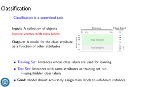
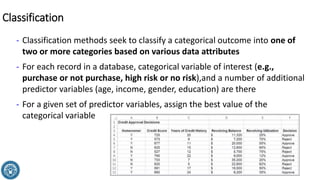
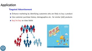
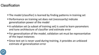
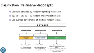
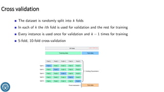
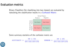
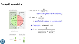
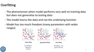
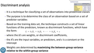
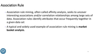
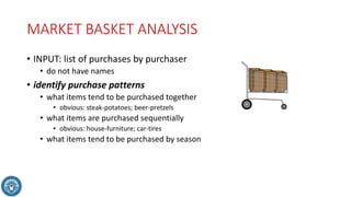
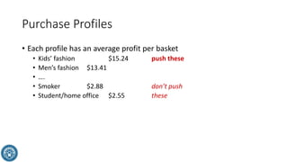
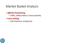
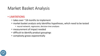
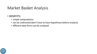
5. Classification
- Classification methods seek to classify a categorical outcome into one of
two or more categories based on various data attributes
- For each record in a database, categorical variable of interest (e.g.,
purchase or not purchase, high risk or no risk),and a number of additional
predictor variables (age, income, gender, education) are there
- For a given set of predictor variables, assign the best value of the
categorical variable
5
10. ▪ The model (classifier) is learned by finding patterns in training set
▪ Performance on training set does not (necessarily) indicate
generalization power of the model
▪ A validation set (a subset of training set) is used to learn parameters
and tune architecture of classifier and estimate error
▪ For generalization of the model, validation set must be representative
of the input instances
▪ Since test set is never used during training, it provides an unbiased
estimate of generalization error
Classification
11. Using Training and Validation Data
- Most data-mining projects use large volumes of data
- Before building a model, partition the data into a training data set and a validation data set
- Training data sets have known outcomes and are used to “teach” a data-mining algorithm
- To get a more realistic estimate of how the model would perform with unseen data, set aside a part
of the original data into a validation data set and not use it in the training process
- The validation data set is often used to fine-tune models
- When a model is finally chosen, its accuracy with the validation data set is still an optimistic estimate
of how it would perform with unseen data
- Data miners often set aside another portion of data, which is used neither in training nor in
validation. This set is known as the test data set
- The accuracy of the model on the test data gives a realistic estimate of the performance of the
model on completely unseen data
11
16. Overfitting
- The phenomenon when model performs very well on training data
but does not generalize to testing data
- The model learns the data and not the underlying function
- Model has too much freedom (many parameters with wider
ranges)
16
19. Decision tree
- Fundamentally, an if-then rule set for
classifying objects
- Builds model in the form of a tree
structure
- To classify a test instance x traverse the
tree from root to leaf
- Take branches at internal nodes according
to results of their tests
- Predict the class label at the leaf node
reached
19
20. Classification methods
- In this database, the categorical variable of interest is the decision to
approve or reject a credit application
- The remaining variables are the predictor variables
- Code the Homeowner and Decision fields numerically. Homeowner
attribute “Y” as 1 and “N” as 0; similarly, Decision attribute “Approve” as 1
and “Reject” as 0
20
22. Example
- To develop an intuitive understanding of classification, consider only the
credit score and years of credit history as predictor variables
- The large bubbles represent the applicants whose credit applications were
rejected; the small bubbles represent those that were approved
- There appears to be a clear separation of the points
- When the credit score is greater than 640, the applications were approved,
but most applications with credit scores of 640 or less were rejected
- Thus, a simple classification rule: approve an application with a credit
score greater than 640
22
23. Example
- Another way of classifying the groups is to use both the credit score and
years of credit history by visually drawing a straight line to separate the
groups
- This line passes through the points (763, 2) and (595, 18). Using a little
algebra, it can be calculated the equation of the line as
years = −0.095 × credit score + 74.66
- Therefore, a different classification rule can be obtained: whenever
years + 0.095 × credit score ≤ 74.66,
the application is rejected; otherwise, it is approved.
23
y = mx + c
m = (y2 – y1)/(x2 – x1)
x-x1 = m(y-y1)
25. Classifying New Data
- The purpose of developing a classification model is to be able to classify
new data. After a classification scheme is chosen and the best model is
developed based on existing data, use the predictor variables as inputs to
the model to predict the output
- Simple credit-score rule that a score of more than 640 is needed??
- If second rule having both the credit score and years of credit history??
25
26. Discriminant analysis
- It is a technique for classifying a set of observations into predefined classes
- The purpose is to determine the class of an observation based on a set of
predictor variables
- Based on the training data set, the technique constructs a set of linear
functions of the predictors, known as discriminant functions, which have
the form:
- where the b’s are weights, or discriminant coefficients,
- the X’s are the input variables, or predictors, and c is a constant or the
intercept
- Weights are determined by maximizing the between-group variance
relative to the within-group variance 26
27. Classifying Credit Decisions Using Discriminant Analysis
- The discriminant analysis procedure incorporates prior assumptions about
how frequently the different classes occur. Three options:
- According to relative occurrences in training data: This option assumes
that the probability of encountering a particular category is the same as the
frequency with which it occurs in the training data
- Use equal prior probabilities: This option assumes that all categories occur
with equal probability
- User specified prior probabilities. This option is available only if the output
variable has two categories
27
28. Classifying Credit Decisions Using Discriminant Analysis
- The classification (discriminant) functions for the two categories. For
category 1 (approve the loan application), the discriminant function is
- L(1) = −137.48 + 32.295 × homeowner + 0.286 × credit score + 0.833 ×
years of credit history + 0.00010274 × revolving balance + 128.248 ×
revolving utilization
- For category 0 (reject the loan application), the discriminant function is
- L(0) = −157.2 + 30.747 × homeowner + 0.289 × credit score + 0.473 × years
of credit history + 0.0004716 × revolving balance + 167.7 × revolving
utilization
28
29. Discriminant analysis
- Like many statistical procedures, discriminant analysis requires certain
assumptions, such as normality of the independent variables
- The normality assumption is often violated in practice, but the method is
generally robust to violations of the assumptions
- The lateron we will study a technique, called logistic regression, does not
rely on these assumptions, making it preferred by many analytics
practitioners
29
30. Association Rule
- Association rule mining, often called affinity analysis, seeks to uncover
interesting associations and/or correlation relationships among large sets of
data. Association rules identify attributes that occur frequently together in
a given data set
- A typical and widely used example of association rule mining is market
basket analysis.
30
31. Market basket analysis
- For example, supermarkets routinely collect data using bar-code scanner by
a customer for a single-purchase transaction
- Such databases consist of a large number of transaction records
- Managers would be interested to know if certain groups of items are
consistently purchased together
- They could use these data for adjusting store layouts (placing items
optimally with respect to each other), for cross-selling, for promotions, for
catalog design, and to identify customer segments based on buying
patterns
- Association rule mining is how companies such as Netflix and Amazon.com
make recommendations based on past movie rentals or item purchases31
32. MARKET BASKET ANALYSIS
• INPUT: list of purchases by purchaser
• do not have names
• identify purchase patterns
• what items tend to be purchased together
• obvious: steak-potatoes; beer-pretzels
• what items are purchased sequentially
• obvious: house-furniture; car-tires
• what items tend to be purchased by season
33. Market Basket Analysis
• Categorize customer purchase behavior
• identify actionable information
• purchase profiles
• profitability of each purchase profile
• use for marketing
• layout or catalogs
• select products for promotion
• space allocation, product placement
34. Market Basket Analysis
• Market Basket Benefits
• selection of promotions, merchandising strategy
• sensitive to price: Italian entrees, pizza, pies, Oriental entrees, orange juice
• uncover consumer spending patterns
• correlations: orange juice & waffles
• joint promotional opportunities
35. Market Basket Analysis
• Retail outlets
• Telecommunications
• Banks
• Insurance
• link analysis for fraud
• Medical
• symptom analysis
36. Market Basket Analysis
• Chain Store Age Executive (1995)
1) Associate products by category
2) what % of each category was in each market basket
• Customers shop on personal needs, not on product groupings
40. Purchase Profiles
• Each profile has an average profit per basket
• Kids’ fashion $15.24 push these
• Men’s fashion $13.41
• ….
• Smoker $2.88 don’t push
• Student/home office $2.55 these
41. Market Basket Analysis
• Affinity Positioning
• coffee, coffee makers in close proximity
• Cross-Selling
• cold medicines, orange juice
42. Market Basket Analysis
• LIMITATIONS
• takes over ~18 months to implement
• market basket analysis only identifies hypotheses, which need to be tested
• neural network, regression, decision tree analyses
• measurement of impact needed
• difficult to identify product groupings
• complexity grows exponentially
43. Market Basket Analysis
• BENEFITS:
• simple computations
• can be undirected (don’t have to have hypotheses before analysis)
• different data forms can be analyzed