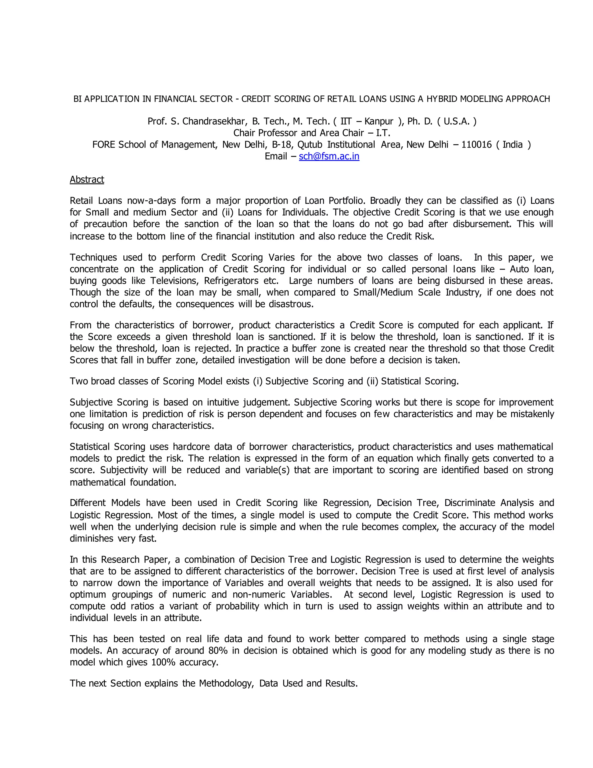
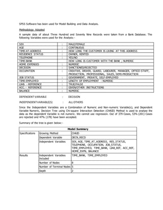
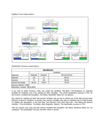
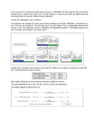
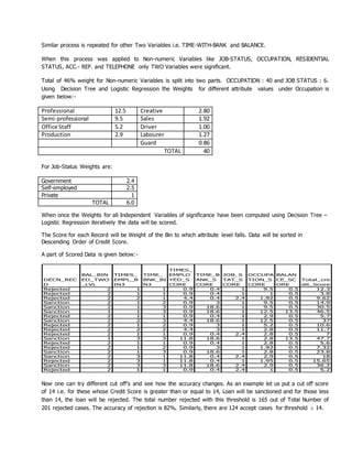
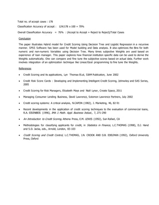
This document discusses using a hybrid modeling approach combining decision trees and logistic regression to develop a credit scoring model for retail loans. It presents a case study where this approach was tested on real loan data. Key points: - A decision tree was first used to identify important borrower characteristics and assign initial weights. Logistic regression was then used to compute odds ratios and assign refined weights within each characteristic. - This iterative process determined weights for both numeric factors like time at bank and non-numeric factors like occupation. Binning of numeric variables was done automatically using additional decision trees. - When tested on loan application data, the hybrid model achieved a classification accuracy of around 80%, higher than single models. This approach provides an

1. BI APPLICATION IN FINANCIAL SECTOR - CREDIT SCORING OF RETAIL LOANS USING A HYBRID MODELING APPROACH
Prof. S. Chandrasekhar, B. Tech., M. Tech. ( IIT – Kanpur ), Ph. D. ( U.S.A. )
Chair Professor and Area Chair – I.T.
FORE School of Management, New Delhi, B-18, Qutub Institutional Area, New Delhi – 110016 ( India )
Email – sch@fsm.ac.in
Abstract
Retail Loans now-a-days form a major proportion of Loan Portfolio. Broadly they can be classified as (i) Loans
for Small and medium Sector and (ii) Loans for Individuals. The objective Credit Scoring is that we use enough
of precaution before the sanction of the loan so that the loans do not go bad after disbursement. This will
increase to the bottom line of the financial institution and also reduce the Credit Risk.
Techniques used to perform Credit Scoring Varies for the above two classes of loans. In this paper, we
concentrate on the application of Credit Scoring for individual or so called personal loans like – Auto loan,
buying goods like Televisions, Refrigerators etc. Large numbers of loans are being disbursed in these areas.
Though the size of the loan may be small, when compared to Small/Medium Scale Industry, if one does not
control the defaults, the consequences will be disastrous.
From the characteristics of borrower, product characteristics a Credit Score is computed for each applicant. If
the Score exceeds a given threshold loan is sanctioned. If it is below the threshold, loan is sanctioned. If it is
below the threshold, loan is rejected. In practice a buffer zone is created near the threshold so that those Credit
Scores that fall in buffer zone, detailed investigation will be done before a decision is taken.
Two broad classes of Scoring Model exists (i) Subjective Scoring and (ii) Statistical Scoring.
Subjective Scoring is based on intuitive judgement. Subjective Scoring works but there is scope for improvement
one limitation is prediction of risk is person dependent and focuses on few characteristics and may be mistakenly
focusing on wrong characteristics.
Statistical Scoring uses hardcore data of borrower characteristics, product characteristics and uses mathematical
models to predict the risk. The relation is expressed in the form of an equation which finally gets converted to a
score. Subjectivity will be reduced and variable(s) that are important to scoring are identified based on strong
mathematical foundation.
Different Models have been used in Credit Scoring like Regression, Decision Tree, Discriminate Analysis and
Logistic Regression. Most of the times, a single model is used to compute the Credit Score. This method works
well when the underlying decision rule is simple and when the rule becomes complex, the accuracy of the model
diminishes very fast.
In this Research Paper, a combination of Decision Tree and Logistic Regression is used to determine the weights
that are to be assigned to different characteristics of the borrower. Decision Tree is used at first level of analysis
to narrow down the importance of Variables and overall weights that needs to be assigned. It is also used for
optimum groupings of numeric and non-numeric Variables. At second level, Logistic Regression is used to
compute odd ratios a variant of probability which in turn is used to assign weights within an attribute and to
individual levels in an attribute.
This has been tested on real life data and found to work better compared to methods using a single stage
models. An accuracy of around 80% in decision is obtained which is good for any modeling study as there is no
model which gives 100% accuracy.
The next Section explains the Methodology, Data Used and Results.

2. SPSS Software has been used for Model Building and Data Analysis.
Methodology Adopted
A sample data of about Three Hundred and Seventy Nine Records were taken from a Bank Database. The
following Variables were used for the Analysis:-
SEX : MALE/FEMALE
AGE : CONTINUOUS
TIME-AT-ADDRESS : HOW LONG THE CUSTOMER IS LIVING AT THIS ADDRESS
RESIDENCE STATUS : OWNER, RENTED
TELEPHONE : YES/NO
TIME-BANK HOW LONG IS CUSTOMER WITH THE BANK ; NUMERIC
HOME EXPENSES : NUMERIC
DECISION : SANCTIONED/REJECTED
OCCUPATION : CREATIVE, DRIVER, GUARD, LABOURER, MANAGER, OFFICE-STAFF,
PRODUCTION, PROFESSIONAL, SALES, SEMI-PRODUCTION
JOB STATUS : GOVERNMENT, PRIVATE, SELF-EMPLOYED
TIME-EMPLOYED : LENGTH OF EMPLOYMENT - NUMERIC
LIAB. - REFERENCE : TRUE/FALSE
ACC. - REFERENCE : GIVEN/OTHER INSTRUCTIONS
BALANCE : NUMERIC
DEPENDENT VARIABLE : DECISION
INDEPENDENTVARIABLE(S) : ALL OTHERS
Since the Independent Variables are a Combination of Numeric and Non-numeric Variable(s), and Dependent
Variable Numeric, Decision Tree using Chi-square Interaction Detection (CHAID) Method is used to analyse the
data as the dependent Variable is not numeric. We cannot use regression. Out of 379 Cases, 53% (201) Cases
are rejected and 47% (178) have been accepted.
Summary of the tree is given below:-
Model Summary
Specifications Growing Method CHAID
Dependent Variable DECN_RECD
Independent Variables SEX, AGE, TIME_AT_ADDRESS, RES_STATUS,
TELEPHONE, OCCUPATION, JOB_STATUS,
TIME_EMPLOYED, TIME_BANK, LIAB_REF, ACC_REF,
HOME_EXPN, BALANCE
Results Independent Variables
Included
TIME_BANK, TIME_EMPLOYED
Number of Nodes 8
Number of Terminal Nodes 5
Depth 2

3. Graphical Tree is shown below:-
Classification Accuracy is given below:-
Classification
Observed
Predicted
Rejected Sanction Percent Correct
Rejected 178 23 88.6%
Sanction 74 104 58.4%
Overall Percentage 66.5% 33.5% 74.4%
Growing Method: CHAID
Dependent Variable: DECN_RECD
If you look at Model Summary Table, the model has identified Time-Bank, Time-Employed, as important
Variables for Prediction and it has rejected all other Variables. The overall classification accuracy is 74%. All
Non-numeric Variables like Occupation, Job Status, Residential Status etc. are ignored.
One reason for rejecting all other Non-numeric Variables may be due to sample size of the data set and heavy
influence of Numeric Variables. In practice, Non-numeric Variables also play an important role in Credit Scoring.
To validate this assumption, in the next step, Two Decision Trees have been built – One taking only Numeric
Variables : Time-At-Address, Time-Bank, Home-Expenses, Balance. The classification accuracy is 77%.
Then for Second Tree using only Non-numeric Variables like Occupation, Job Status, Residence Status etc. are
considered. The Classification accuracy was 66% which is not low.

4. Hence one can include both Numeric and Non-numeric Variable but with a slightly higher weightage for Numeric
compared to Non-numeric Variables. The weights will be inversely proportional to error i.e. if the error is high
weight will be less and vice-versa.
So, the overall weightage assigned to Numeric Variables are : (77/(77+66)) x 100 = 54% ; it is (66/(77+66)) x
100 = 46%.
The next step is to assign Individual Weights to different levels within Numeric and Non-numeric Variables
keeping overall weights to 54% and 46%.
Logistic Regression is used for assigning Individual Weights.
Logistic Regression gives a functional relation between Dependent and Independent Variables. The only
difference between Logistic Regression and Usual Regression is the Dependent Variable is categorical and has
only two states of nature like Loan Application Accepted/Rejected, Person defaulting a loan/not defaulting etc.
The functional form can be expressed as:
α0 , α1 , α2 , …………………..are called the Logit Coefficients and will be estimated using sample data using
maximum likelihood estimation.
Out of all the Independent Variables taken for model building, I have explained below methodology of assigning
Individual Weights for different attribute level values. One example for Numeric Variable and another for Non-
numeric Variable. This methodology is repeated for all other Numeric and Non-numeric Variables.
When all the Numeric Variables are taken as Independent Variable(s), and DECISION as Dependent Variable,
Logistic Regression is run. Based on the significance the following Variables are retained:-
TIME-BANK (1.53) TIME-EMPLOYED (1.20) BALANCE(1.0)
The numbers in the bracket indicate the odd ratio and all are significant at 5%. Put alternatively what it means is
these Coefficients are correct 95% of time. Only 5% of time they may be wrong. COX_NELL R Square of about
0.4. Validates the Hypothesis, that Logistic Regression fits the data. If value of COX_NELL R Square is below
0.05 one can conclude Logistic Regression does not fit the data.
Out of Total Weight of 54% assigned to all Numeric Variables, the break-up of Weights for THREE significant
Numeric Variables are worked out as follows using the Logit Coefficients:-
TIME-BANK = (1.53/(1.53+1.20+1.0))x54=22
TIME-EMPLOYED = (1.20/(1.53+1.20+1.0))x54=17
BALANCE = (1.0/1.53+1.20+1.0))X54=15
ProbabilityLn
Loan rejected
Loan sanctioned
= α0+α1*Time-at-Address+α2*Time-employed+

5. At the next level let us take one Variable used in Scoring i.e. TIME-BANK. The total weight for this is 22 and this
Variable takes on values in the range: 0-67. The total weight of 22 needs to be broken into different bins and
the binning should be automatic instead of person dependent.
For this, the methodology used is as follows:-
The histogram was displayed and using Visual binning techniques the Variable TIME-BANK was binned into 5
bins. This may not be optimum. The next step was to use the Decision Tree to automatically determine the
number of bins. The Dependent Variable is DECISION and Independent Variable is TIME-BANK grouped into 5
bins. The output of the Decision Tree is given below:-
FIGURE : 2
Looking at the Tree output shown above it is clear that only THREE bins are optimum compared to manual FIVE
bins. The following bins are given as under:-
TIME-EMPLOYED ≤ 1.0 Bin1
1.0 < TIME-EMPLOYED ≤ 3.0 Bin2
TIME-EMPLOYED > 3.0 Bin3
Again Logistic Regression is used to determine Individual Weights for each bin.
The Logit Coefficients for Bin 1, Bin 2 and Bin 3 are 0.4, 3.0 and 19.0 respectively.
The weights assigned to different bins are:

6. Similar process is repeated for other Two Variables i.e. TIME-WITH-BANK and BALANCE.
When this process was applied to Non-numeric Variables like JOB-STATUS, OCCUPATION, RESIDENTIAL
STATUS, ACC.- REF. and TELEPHONE only TWO Variables were significant.
Total of 46% weight for Non-numeric Variables is split into two parts. OCCUPATION : 40 and JOB STATUS : 6.
Using Decision Tree and Logistic Regression the Weights for different attribute values under Occupation is
given below:-
Professional 12.5 Creative 2.80
Semi-professional 9.5 Sales 1.92
Office Staff 5.2 Driver 1.00
Production 2.9 Labourer 1.27
Guard 0.86
TOTAL 40
For Job-Status Weights are:
Government 2.4
Self-employed 2.5
Private 1
TOTAL 6.0
When once the Weights for all Independent Variables of significance have been computed using Decision Tree –
Logistic Regression iteratively the data will be scored.
The Score for each Record will be Weight of the Bin to which attribute level falls. Data will be sorted in
Descending Order of Credit Score.
A part of Scored Data is given below:-
DECN_REC
D
BAL_BIN
ED_TWO
_LVL
TIMES_
EMPL_B
IN3
TIME_
BNK_BI
N3
TIMES_
EMPLO
YED_S
CORE
TIME_B
ANK_S
CORE
JOB_S
TAT_S
CORE
OCCUPA
TION_S
CORE
BALAN
CE_SC
ORE
Total_cre
dit_Score
Rejected 2 1 1 0.9 0.4 1 9.5 0.5 12.3
Rejected 2 1 1 0.9 0.4 1 1 0.5 3.8
Rejected 2 2 1 4.4 0.4 2.4 1.92 0.5 9.62
Sanction 2 1 2 0.9 3 1 9.5 0.5 14.9
Sanction 2 1 3 0.9 18.6 1 9.5 0.5 30.5
Sanction 1 1 3 0.9 18.6 1 12.5 13.5 46.5
Rejected 2 1 1 0.9 0.4 1 2.9 0.5 5.7
Sanction 2 2 3 4.4 18.6 1 12.5 0.5 37
Rejected 2 1 2 0.9 3 1 5.2 0.5 10.6
Rejected 2 2 2 4.4 3 1 2.8 0.5 11.7
Rejected 2 1 1 0.9 0.4 2.4 2.8 0.5 7
Sanction 1 3 3 11.8 18.6 1 2.8 13.5 47.7
Rejected 2 1 1 0.9 0.4 1 2.8 0.5 5.6
Rejected 2 1 2 0.9 3 1 1.92 0.5 7.32
Sanction 2 1 3 0.9 18.6 1 2.8 0.5 23.8
Sanction 2 3 1 11.8 0.4 2.4 2.9 0.5 18
Rejected 2 3 1 11.8 0.4 1 1.95 0.5 15.65
Sanction 2 3 3 11.8 18.6 2.4 2.9 0.5 36.2
Rejected 2 1 1 0.9 0.4 2.4 1 0.5 5.2
Now one can try different cut off’s and see how the accuracy changes. As an example let us put a cut off score
of 14 i.e. for these whose Credit Score is greater than or equal to 14, Loan will be sanctioned and for those less
than 14, the loan will be rejected. The total number rejected with this threshold is 165 out of Total Number of
201 rejected cases. The accuracy of rejection is 82%. Similarly, there are 124 accept cases for threshold  14.

7. Conclusion
The paper illustrates Hybrid model for Credit Scoring Using Decision Tree and Logistic Regression in a recursive
manner. SPSS Software has been used for Model building and Data analysis. It also optimizes the Bins for both
numeric and non-numeric Variables using Decision Tree. Many times subjective Weights are used based on
experience of loan manager. This paper explores how financial institution specific data can be used to derive the
Weights automatically. One can compare and fine tune the subjective scores based on actual data. Further work
involves integration of an optimization technique like Linear/Goal programming to fine tune the Weights.
References
 Credit Scoring and its applications, Lyn Thomas Et.al, SIAM Publication, June 2002
 Credit Risk Score Cards : Developing and Implementing Intelligent Credit Scoring, Johnwiley and SAS Series,
2005
 Credit Scoring for Risk Managers, Elizabeth Mays and Niall Lynar, Create Space, 2011
 Managing Consumer Lending Business, David Lawrence, Solomon Lawrence Partners, July 2002
 Credit scoring systems: A critical analysis, N.CAPON (1982), J. Marketing, 46, 82-91
 Recent developments in the application of credit scoring techniques to the evaluation of commercial loans,
R.A. EISENBEIS (1996), IMA J. Math. Appl. Business Indust., 7, 271-290
 An Introduction to Credit Scoring, Athena Press, E.M. LEWIS (1992), San Rafael, CA
 Methodologies for classifying applicants for credit, in Statistics in Finance, L.C.THOMAS (1998), D.J. Hand
and S.D. Jacka, eds., Arnold, London, 83-103
 Credit Scoring and Credit Control, L.C.THOMAS, J.N. CROOK AND D.B. EDELMAN (1992), Oxford University
Press, Oxford
Total no. of accept cases : 178
Classification Accuracy of accept : 124/178 x 100 = 70%
Overall Classification Accuracy = 76% : (Accept to Accept + Reject to Reject)/Total Cases