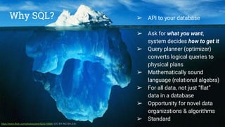
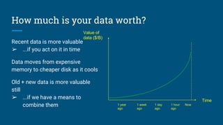
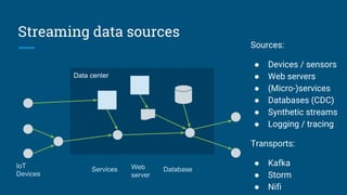
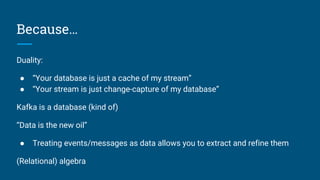
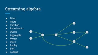
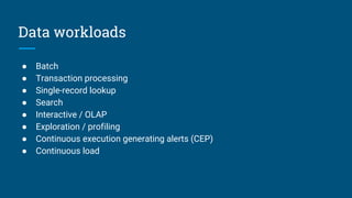
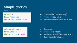
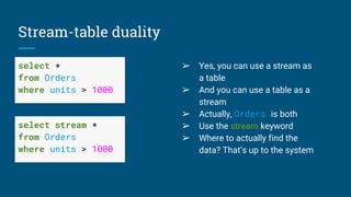
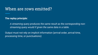
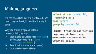
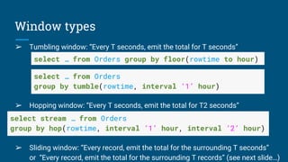
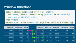
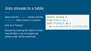
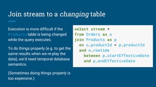
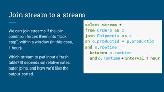
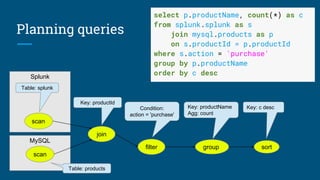
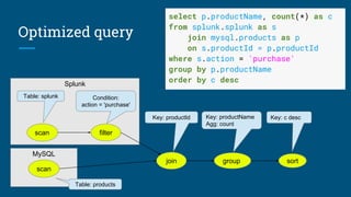
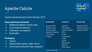
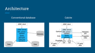
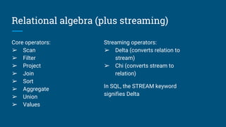
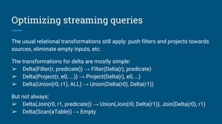
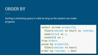
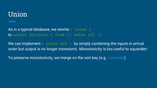
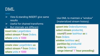
The document discusses Streaming SQL, emphasizing its role in managing and querying streaming data alongside traditional relational data. It details query planning, the duality of streams and tables, and the importance of time-sensitive data, while also covering different windowing techniques and aggregation methods. Additionally, it highlights the need for optimizing streaming queries to achieve high-quality results in real-time applications.

1. Streaming SQL
Julian Hyde

2. @julianhyde
SQL
Query planning
Query federation
OLAP
Streaming
Hadoop
Thanks:
● Milinda Pathirage & Yi Pan (Samza)
● Haohui Mai (Storm)
● Fabian Hueske & Stephan Ewen (Flink)

3. Agenda

4. What? Why?
Agenda

5. What? Why?
I love databases.
Why should I care
about streaming
data?
I love Kafka. Why
would I want to
make it look like a
database?
Agenda

6. Why SQL? ● API to your database
● Ask for what you want,
system decides how to get it
● Query planner (optimizer)
converts logical queries to
physical plans
● Mathematically sound
language (relational algebra)
● For all data, not just data in a
database
● Opportunity for novel data
organizations & algorithms
● Standard
https://www.flickr.com/photos/pere/523019984/ (CC BY-NC-SA 2.0)
➢ API to your database
➢ Ask for what you want,
system decides how to get it
➢ Query planner (optimizer)
converts logical queries to
physical plans
➢ Mathematically sound
language (relational algebra)
➢ For all data, not just “flat”
data in a database
➢ Opportunity for novel data
organizations & algorithms
➢ Standard
Why SQL?

7. How much is your data worth?
Recent data is more valuable
➢ ...if you act on it in time
Data moves from expensive
memory to cheaper disk as it cools
Old + new data is more valuable
still
➢ ...if we have a means to
combine them
Time
Value of
data ($/B)
Now1 hour
ago
1 day
ago
1 week
ago
1 year
ago

8. Data center
Streaming data sources
Sources:
● Devices / sensors
● Web servers
● (Micro-)services
● Databases (CDC)
● Synthetic streams
● Logging / tracing
Transports:
● Kafka
● Storm
● Nifi
IoT
Devices
Services DatabaseWeb
server

9. Because…
Duality:
● “Your database is just a cache of my stream”
● “Your stream is just change-capture of my database”
Kafka is a database (kind of)
“Data is the new oil”
● Treating events/messages as data allows you to extract and refine them
(Relational) algebra

10. Streaming algebra
● Filter
● Route
● Partition
● Round-robin
● Queue
● Aggregate
● Merge
● Store
● Replay
● Sort
● Lookup

11. Data workloads
● Batch
● Transaction processing
● Single-record lookup
● Search
● Interactive / OLAP
● Exploration / profiling
● Continuous execution generating alerts (CEP)
● Continuous load

12. Simple queries
select *
from Products
where unitPrice < 20
select stream *
from Orders
where units > 1000
➢ Traditional (non-streaming)
➢ Products is a table
➢ Retrieves records from -∞ to now
➢ Streaming
➢ Orders is a stream
➢ Retrieves records from now to +∞
➢ Query never terminates

13. Stream-table duality
select *
from Orders
where units > 1000
➢ Yes, you can use a stream as
a table
➢ And you can use a table as a
stream
➢ Actually, Orders is both
➢ Use the stream keyword
➢ Where to actually find the
data? That’s up to the system
select stream *
from Orders
where units > 1000

14. Combining past and future
select stream *
from Orders as o
where units > (
select avg(units)
from Orders as h
where h.productId = o.productId
and h.rowtime > o.rowtime - interval ‘1’ year)
➢ Orders is used as both stream and table
➢ System determines where to find the records
➢ Query is invalid if records are not available

15. The “pie chart” problem
➢ Task: Write a web page summarizing
orders over the last hour
➢ Problem: The Orders stream only
contains the current few records
➢ Solution: Materialize short-term history
Orders over the last hour
Beer
48%
Cheese
30%
Wine
22%
select productId, count(*)
from Orders
where rowtime > current_timestamp - interval ‘1’ hour
group by productId

16. Aggregation and windows
on streams
GROUP BY aggregates multiple rows into sub-
totals
➢ In regular GROUP BY each row contributes
to exactly one sub-total
➢ In multi-GROUP BY (e.g. HOP, GROUPING
SETS) a row can contribute to more than
one sub-total
Window functions leave the number of rows
unchanged, but compute extra expressions for
each row (based on neighboring rows)
Multi
GROUP BY
Window
functions
GROUP BY

17. GROUP BY select stream productId,
floor(rowtime to hour) as rowtime,
sum(units) as u,
count(*) as c
from Orders
group by productId,
floor(rowtime to hour)
rowtime productId units
09:12 100 5
09:25 130 10
09:59 100 3
10:00 100 19
11:05 130 20
rowtime productId u c
09:00 100 8 2
09:00 130 10 1
10:00 100 19 1
not emitted yet; waiting
for a row >= 12:00

18. When are rows emitted?
The replay principle:
A streaming query produces the same result as the corresponding non-
streaming query would if given the same data in a table.
Output must not rely on implicit information (arrival order, arrival time,
processing time, or punctuations)

19. Making progress
It’s not enough to get the right result. We
need to give the right result at the right
time.
Ways to make progress without
compromising safety:
➢ Monotonic columns (e.g. rowtime)
and expressions (e.g. floor
(rowtime to hour))
➢ Punctuations (aka watermarks)
➢ Or a combination of both
select stream productId,
count(*) as c
from Orders
group by productId;
ERROR: Streaming aggregation
requires at least one
monotonic expression in
GROUP BY clause

20. Window types
➢ Tumbling window: “Every T seconds, emit the total for T seconds”
➢ Hopping window: “Every T seconds, emit the total for T2 seconds”
➢
➢ Sliding window: “Every record, emit the total for the surrounding T seconds”
or “Every record, emit the total for the surrounding T records” (see next slide…)
select … from Orders group by floor(rowtime to hour)
select … from Orders
group by tumble(rowtime, interval ‘1’ hour)
select stream … from Orders
group by hop(rowtime, interval ‘1’ hour, interval ‘2’ hour)

21. Window functions
select stream sum(units) over w as units1h,
sum(units) over w (partition by productId) as units1hp,
rowtime, productId, units
from Orders
window w as (order by rowtime range interval ‘1’ hour preceding)
rowtime productId units
09:12 100 5
09:25 130 10
09:59 100 3
10:17 100 10
units1h units1hp rowtime productId units
5 5 09:12 100 5
15 10 09:25 130 10
18 8 09:59 100 3
23 13 10:17 100 10

22. Join stream to a table
Inputs are the Orders stream and the
Products table, output is a stream.
Acts as a “lookup”.
Execute by caching the table in a hash-
map (if table is not too large) and
stream order will be preserved.
select stream *
from Orders as o
join Products as p
on o.productId = p.productId

23. Join stream to a changing table
Execution is more difficult if the
Products table is being changed
while the query executes.
To do things properly (e.g. to get the
same results when we re-play the
data), we’d need temporal database
semantics.
(Sometimes doing things properly is
too expensive.)
select stream *
from Orders as o
join Products as p
on o.productId = p.productId
and o.rowtime
between p.startEffectiveDate
and p.endEffectiveDate

24. Join stream to a stream
We can join streams if the join
condition forces them into “lock
step”, within a window (in this case,
1 hour).
Which stream to put input a hash
table? It depends on relative rates,
outer joins, and how we’d like the
output sorted.
select stream *
from Orders as o
join Shipments as s
on o.productId = p.productId
and s.rowtime
between o.rowtime
and o.rowtime + interval ‘1’ hour

25. Planning queries
MySQL
Splunk
join
Key: productId
group
Key: productName
Agg: count
filter
Condition:
action = 'purchase'
sort
Key: c desc
scan
scan
Table: products
select p.productName, count(*) as c
from splunk.splunk as s
join mysql.products as p
on s.productId = p.productId
where s.action = 'purchase'
group by p.productName
order by c desc
Table: splunk

26. Optimized query
MySQL
Splunk
join
Key: productId
group
Key: productName
Agg: count
filter
Condition:
action = 'purchase'
sort
Key: c desc
scan
scan
Table: splunk
Table: products
select p.productName, count(*) as c
from splunk.splunk as s
join mysql.products as p
on s.productId = p.productId
where s.action = 'purchase'
group by p.productName
order by c desc

27. Apache Calcite
Apache top-level project since October, 2015
Query planning framework
➢ Relational algebra, rewrite rules
➢ Cost model & statistics
➢ Federation via adapters
➢ Extensible
Packaging
➢ Library
➢ Optional SQL parser, JDBC server
➢ Community-authored rules, adapters
Embedded Adapters Streaming
Apache Drill
Apache Hive
Apache Kylin
Apache Phoenix*
Cascading
Lingual
Apache
Cassandra
Apache Spark
CSV
Druid*
In-memory
JDBC
JSON
MongoDB
Splunk
Web tables
Apache Flink*
Apache Samza
Apache Storm
* Under development

28. Architecture
Conventional database Calcite

29. Relational algebra (plus streaming)
Core operators:
➢ Scan
➢ Filter
➢ Project
➢ Join
➢ Sort
➢ Aggregate
➢ Union
➢ Values
Streaming operators:
➢ Delta (converts relation to
stream)
➢ Chi (converts stream to
relation)
In SQL, the STREAM keyword
signifies Delta

30. Optimizing streaming queries
The usual relational transformations still apply: push filters and projects towards
sources, eliminate empty inputs, etc.
The transformations for delta are mostly simple:
➢ Delta(Filter(r, predicate)) → Filter(Delta(r), predicate)
➢ Delta(Project(r, e0, ...)) → Project(Delta(r), e0, …)
➢ Delta(Union(r0, r1), ALL) → Union(Delta(r0), Delta(r1))
But not always:
➢ Delta(Join(r0, r1, predicate)) → Union(Join(r0, Delta(r1)), Join(Delta(r0), r1)
➢ Delta(Scan(aTable)) → Empty

31. ORDER BY
Sorting a streaming query is valid as long as the system can make
progress.
select stream productId,
floor(rowtime to hour) as rowtime,
sum(units) as u,
count(*) as c
from Orders
group by productId,
floor(rowtime to hour)
order by rowtime, c desc

32. Union
As in a typical database, we rewrite x union y
to select distinct * from (x union all y)
We can implement x union all y by simply combining the inputs in arrival
order but output is no longer monotonic. Monotonicity is too useful to squander!
To preserve monotonicity, we merge on the sort key (e.g. rowtime).

33. DML
➢ View & standing INSERT give same
results
➢ Useful for chained transforms
➢ But internals are different
insert into LargeOrders
select stream * from Orders
where units > 1000
create view LargeOrders as
select stream * from Orders
where units > 1000
upsert into OrdersSummary
select stream productId,
count(*) over lastHour as c
from Orders
window lastHour as (
partition by productId
order by rowtime
range interval ‘1’ hour preceding)
Use DML to maintain a “window”
(materialized stream history).

34. Summary: Streaming SQL features
Standard SQL over streams and relations
Streaming queries on relations, and relational queries on streams
Joins between stream-stream and stream-relation
Queries are valid if the system can get the data, with a reasonable latency
➢ Monotonic columns and punctuation are ways to achieve this
Views, materialized views and standing queries

35. Summary: The benefits of streaming SQL
Relational algebra covers needs of data-in-flight and data-at-rest applications
High-level language lets the system optimize quality of service (QoS) and data
location
Give DB tools and traditional users to access streaming data;
give message-oriented tools access to historic data
Combine real-time and historic data, and produce actionable results
Discussion continues at Apache Calcite, with contributions from Samza, Flink,
Storm and others. Please join in!

36. Thank you!
@julianhyde
@ApacheCalcite
http://calcite.apache.org
http://calcite.apache.org/docs/stream.html
“Data in Flight”, Communications of the ACM, January 2010 [article]