Download as PDF, PPTX

![Thank you!
@julianhyde
@ApacheCalcite
http://calcite.apache.org
http://calcite.apache.org/docs/stream.html
“Data in Flight”, Communications of the ACM, January 2010 [article]](https://image.slidesharecdn.com/calcite-streaming-sql-apache-con-2016-160511183202/85/Streaming-SQL-with-Apache-Calcite-34-320.jpg)

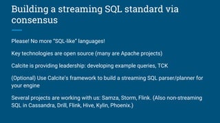
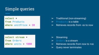
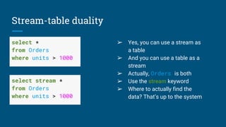
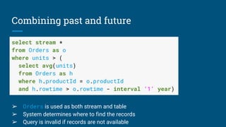
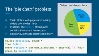
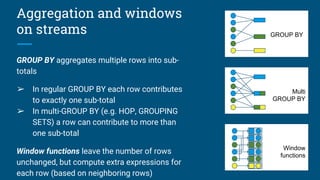
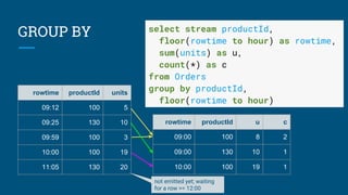
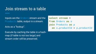
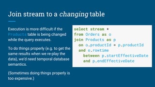
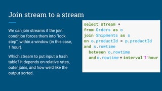
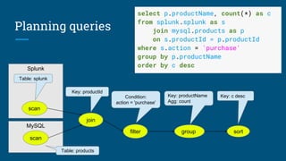
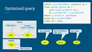
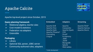
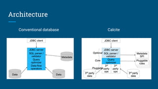
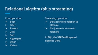
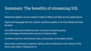
The document discusses the development of Streaming SQL using Apache Calcite, emphasizing its potential for combining real-time and historical data through a standardized SQL approach. It highlights the need for a consensus-driven standard and the roles of various open-source projects like Samza, Storm, and Flink in this ecosystem. The main benefits include optimized query execution for streaming data and improved access for both traditional database and message-oriented applications.