Downloaded 81 times


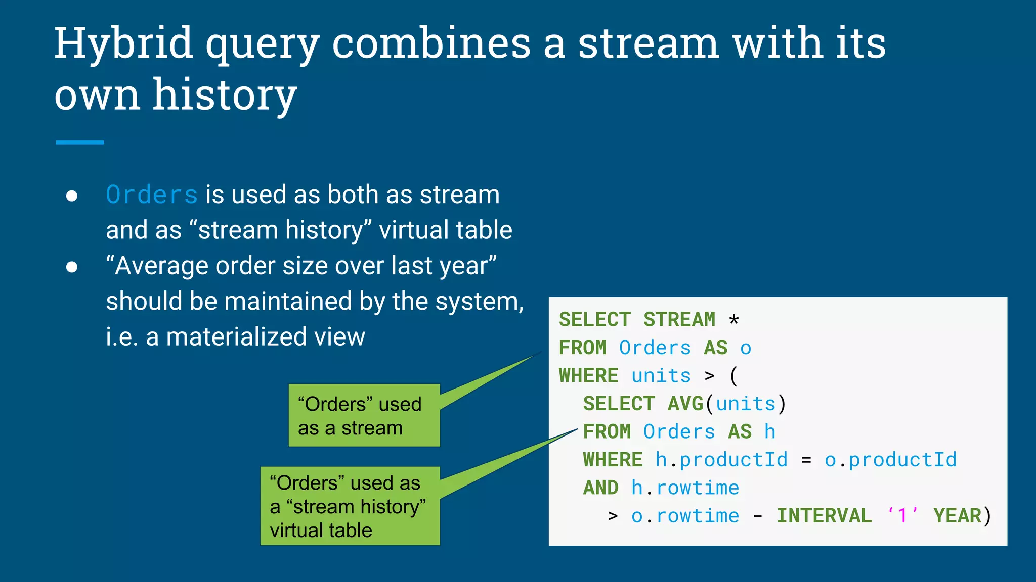
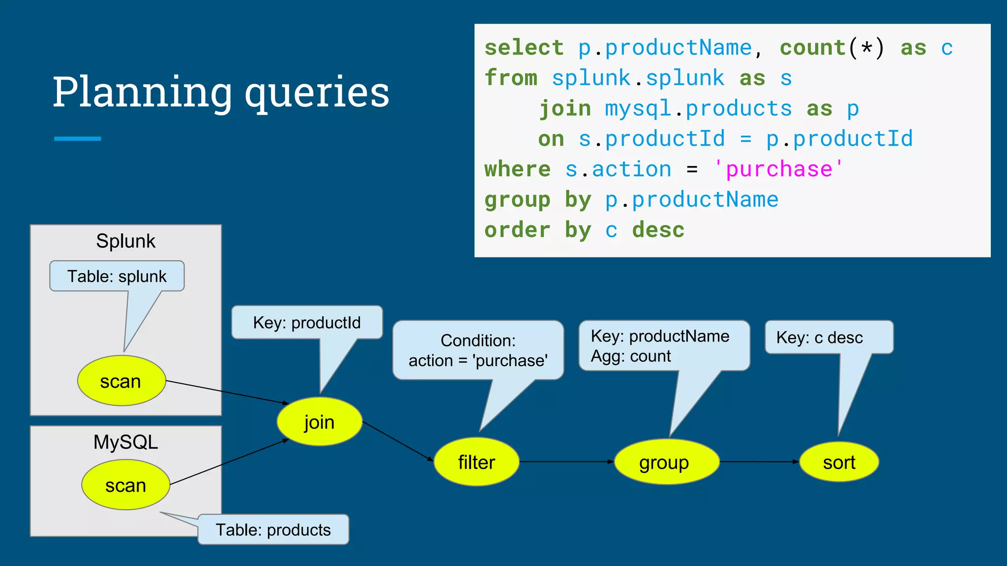
![SELECT d.name, COUNT(*) AS c
FROM Emps AS e
JOIN Depts AS d USING (deptno)
WHERE e.age < 40
GROUP BY d.deptno
HAVING COUNT(*) > 5
ORDER BY c DESC
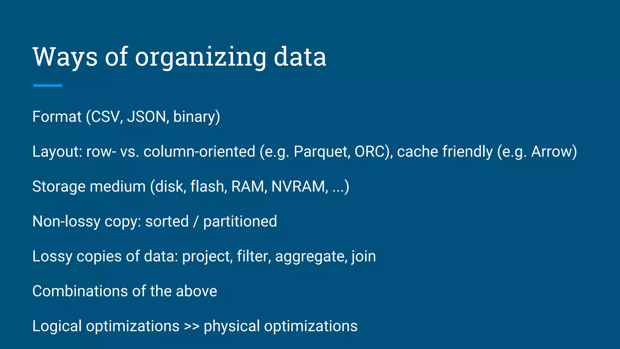
Relational algebra
Based on set theory, plus operators:
Project, Filter, Aggregate, Union, Join,
Sort
Requires: declarative language (SQL),
query planner
Original goal: data independence
Enables: query optimization, new
algorithms and data structures
Scan [Emps] Scan [Depts]
Join [e.deptno = d.deptno]
Filter [e.age < 30]
Aggregate [deptno, COUNT(*) AS c]
Filter [c > 5]
Project [name, c]
Sort [c DESC]](https://image.slidesharecdn.com/calcite-data-eng-2017-171030074234/75/Don-t-optimize-my-queries-optimize-my-data-4-2048.jpg)

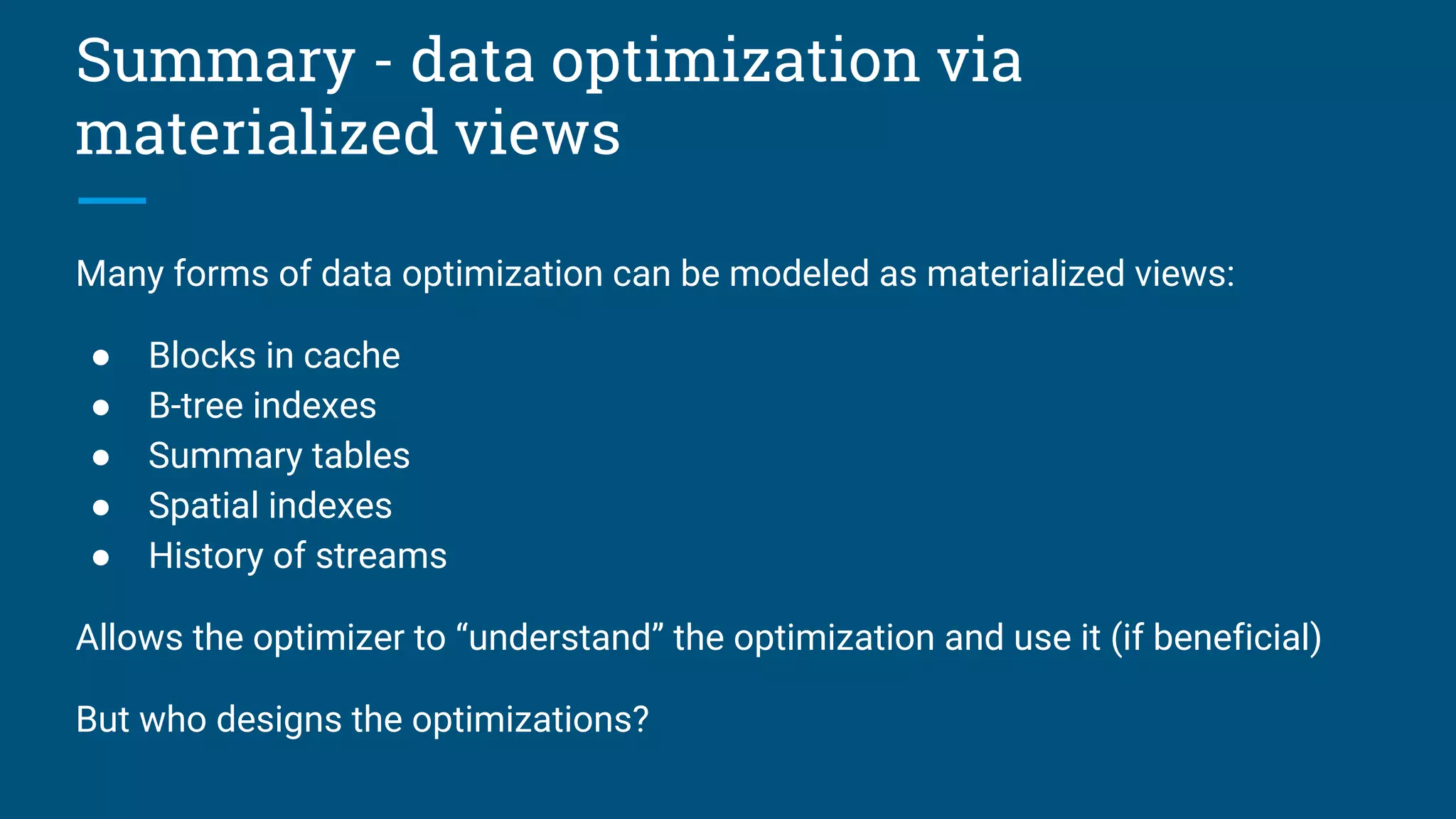
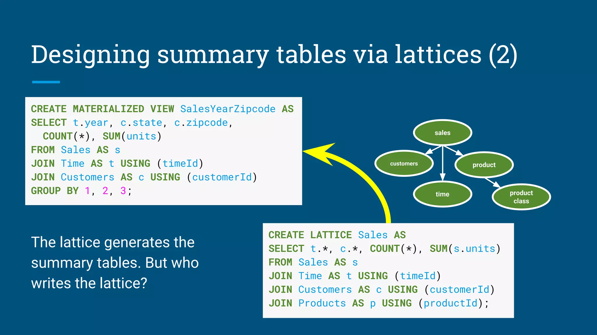
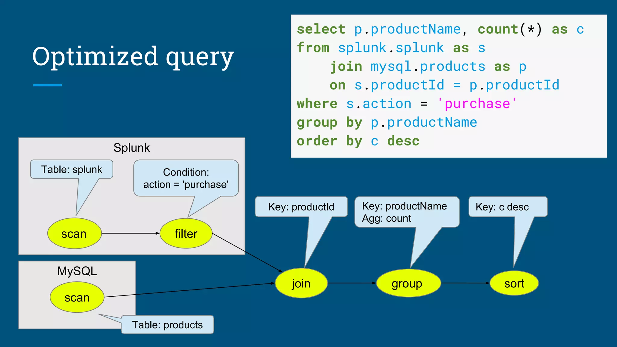
![Materialized view
CREATE MATERIALIZED
VIEW EmpsByDeptno AS
SELECT deptno, name, deptno
FROM Emp
ORDER BY deptno, name;
Scan [Emps]
Scan [EmpsByDeptno]
Sort [deptno, name]
empno name deptno
100 Fred 20
110 Barney 10
120 Wilma 30
130 Dino 10
deptno name empno
10 Barney 100
10 Dino 130
20 Fred 20
30 Wilma 30
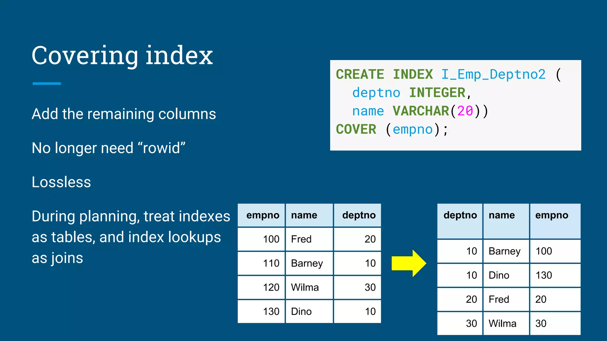
As a materialized view, an
index is now just another
table
Several tables contain the
information necessary to
answer the query - just pick
the best](https://image.slidesharecdn.com/calcite-data-eng-2017-171030074234/75/Don-t-optimize-my-queries-optimize-my-data-12-2048.jpg)

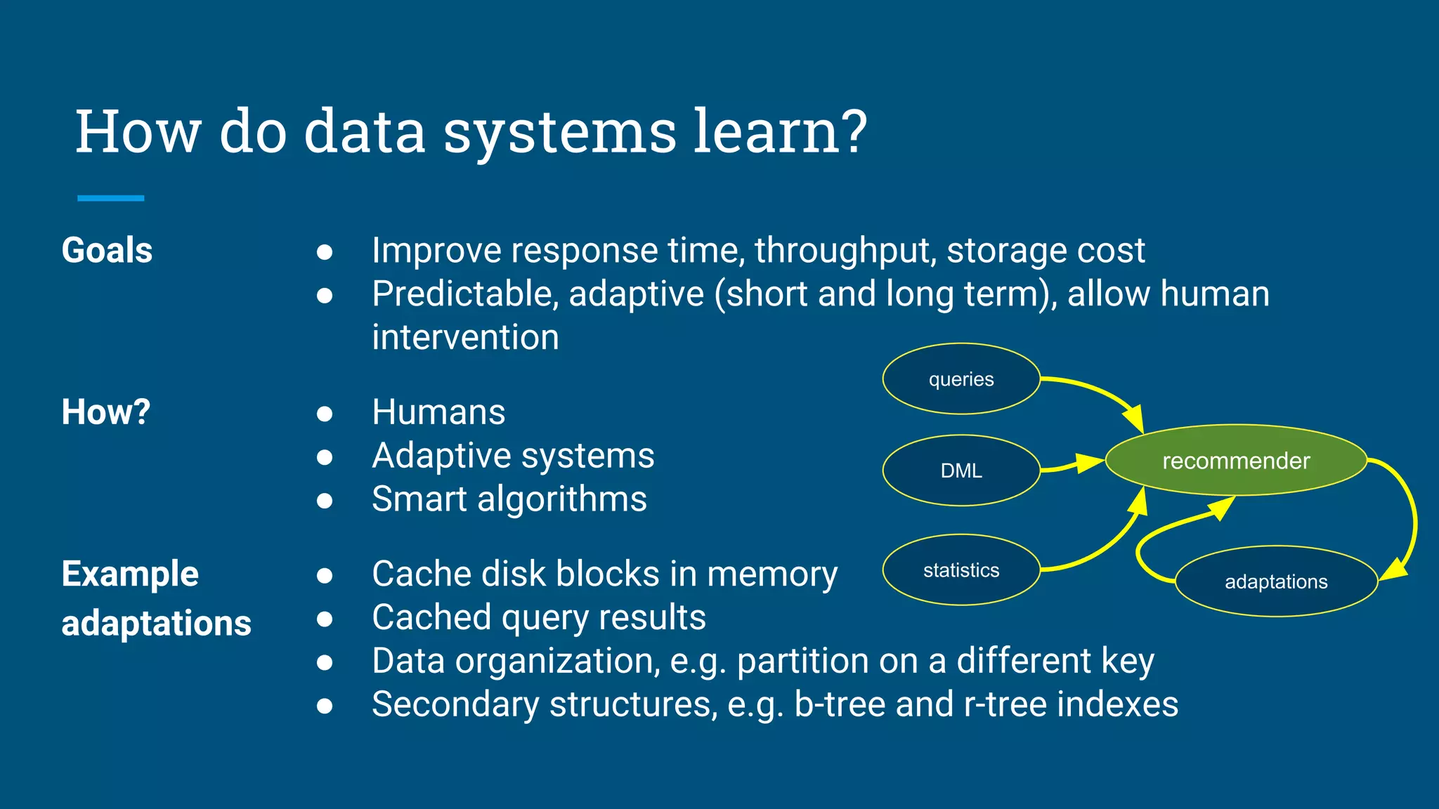
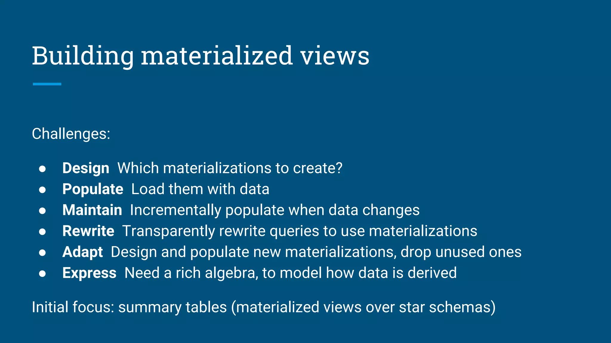
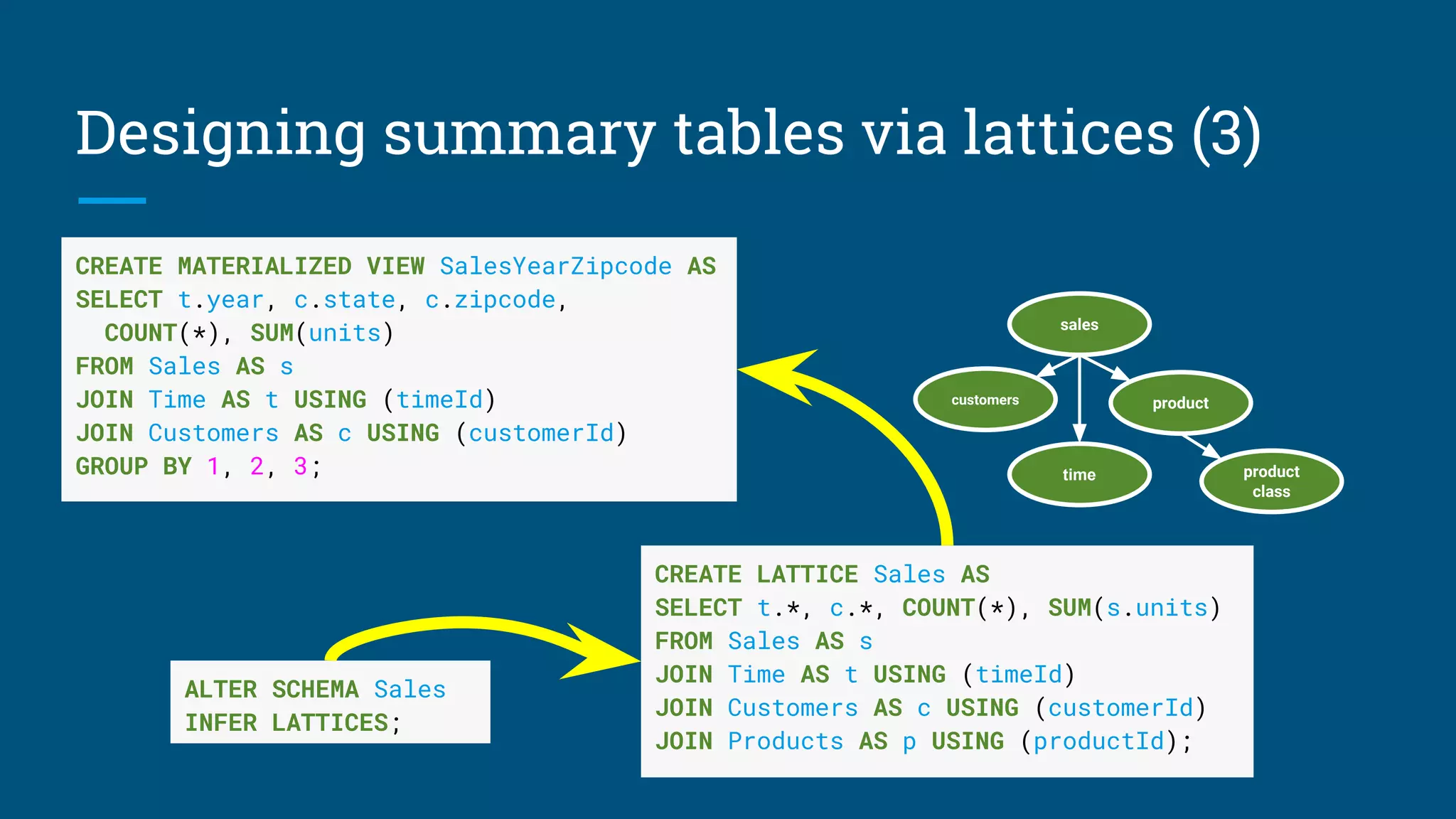
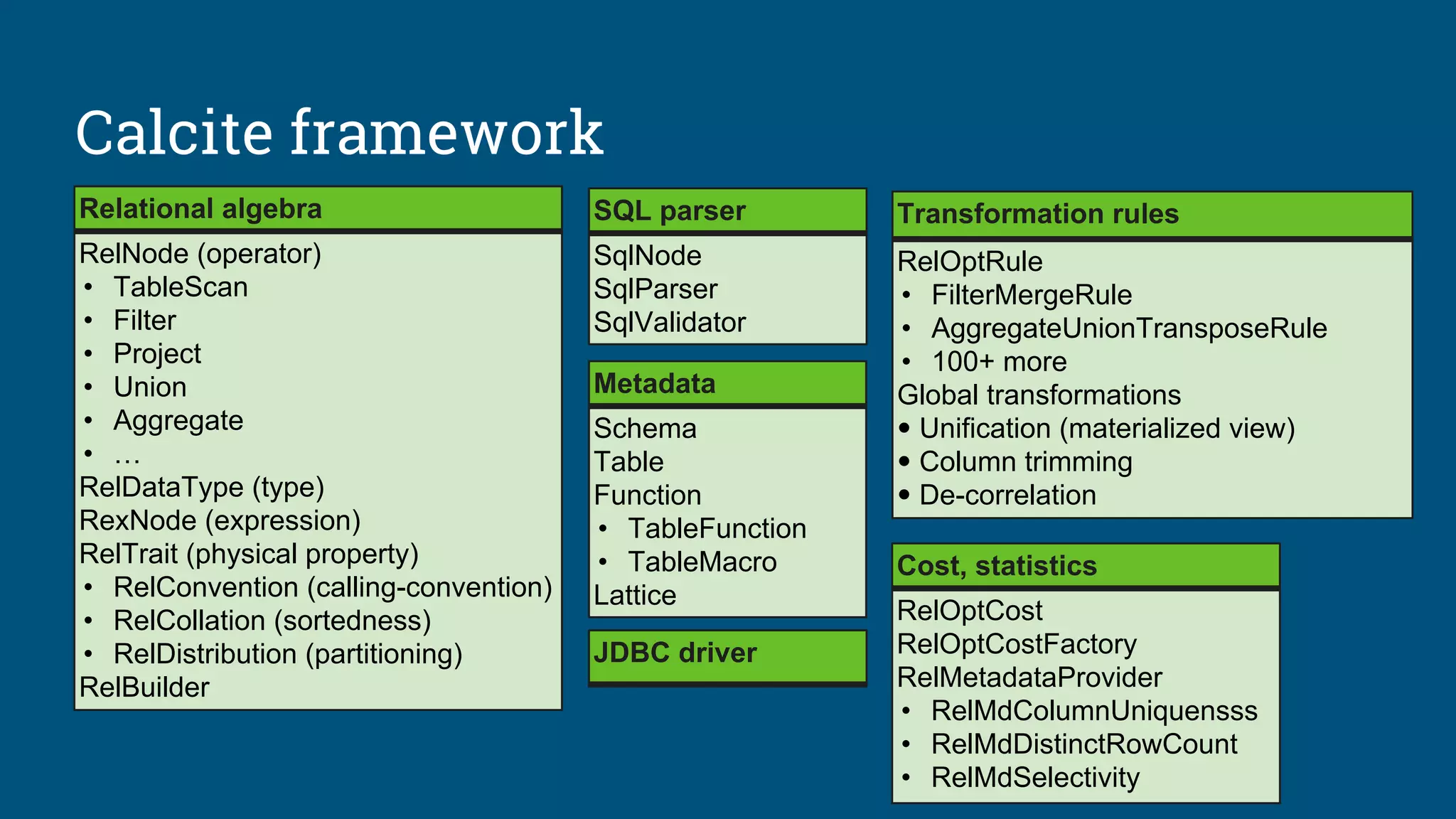
![Algorithm: Design summary tables
Given a database with 30 columns, 10M rows. Find X summary tables with under
Y rows that improve query response time the most.
AdaptiveMonteCarlo algorithm [1]:
● Based on research [2]
● Greedy algorithm that takes a combination of summary tables and tries to
find the table that yields the greatest cost/benefit improvement
● Models “benefit” of the table as query time saved over simulated query load
● The “cost” of a table is its size
[1] org.pentaho.aggdes.algorithm.impl.AdaptiveMonteCarloAlgorithm
[2] Harinarayan, Rajaraman, Ullman (1996). “Implementing data cubes efficiently”](https://image.slidesharecdn.com/calcite-data-eng-2017-171030074234/75/Don-t-optimize-my-queries-optimize-my-data-26-2048.jpg)
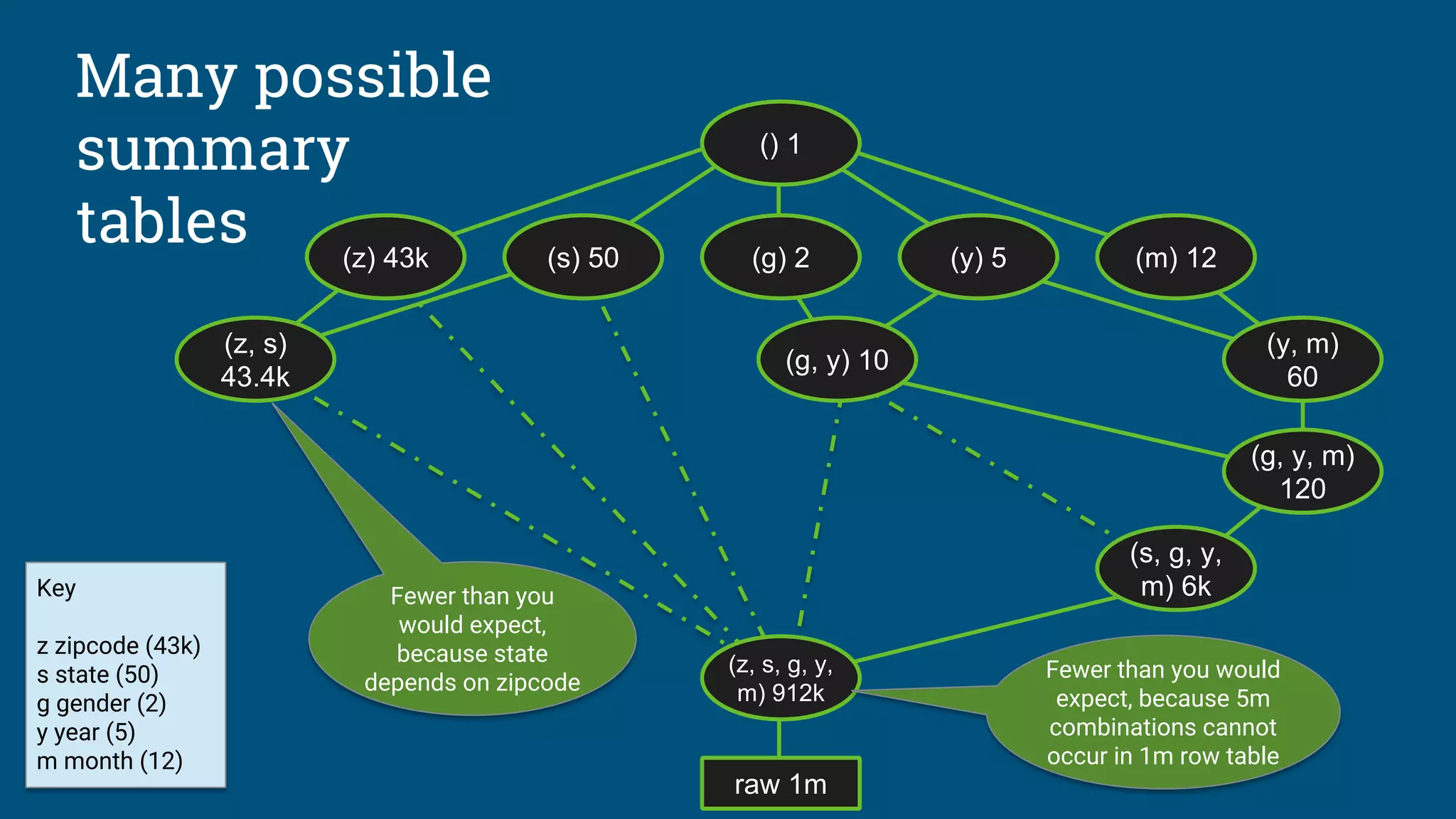
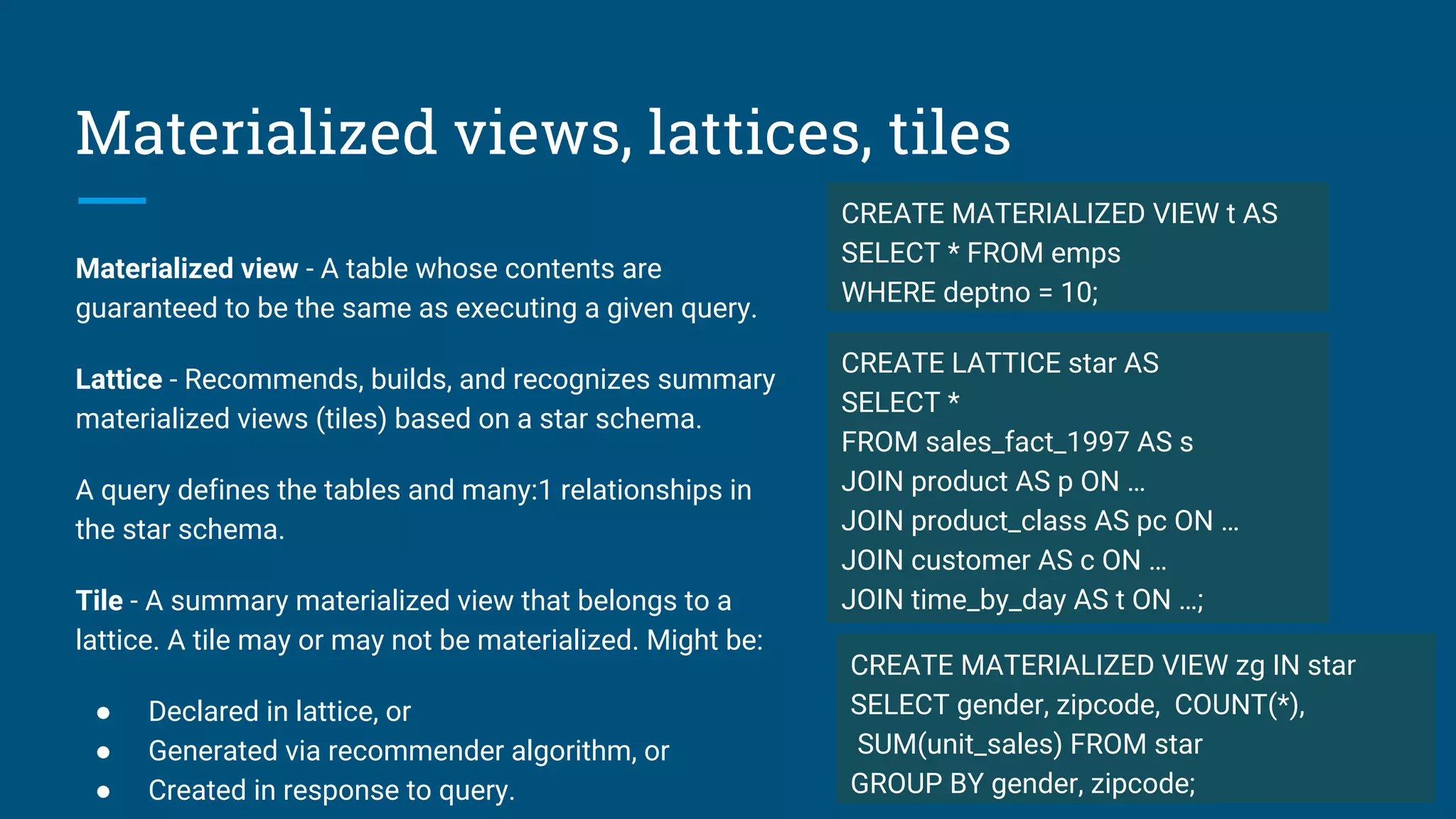
![Data profiling
Algorithm needs count(distinct a, b, ...) for each combination of attributes:
● Previous example had 25
= 32 possible tables
● Schema with 30 attributes has 230
(about 109
) possible tables
● Algorithm considers a significant fraction of these
● Approximations are OK
Attempts to solve the profiling problem:
1. Compute each combination: scan, sort, unique, count; repeat 230
times!
2. Sketches (HyperLogLog)
3. Sketches + parallelism + information theory [CALCITE-1616]](https://image.slidesharecdn.com/calcite-data-eng-2017-171030074234/75/Don-t-optimize-my-queries-optimize-my-data-28-2048.jpg)
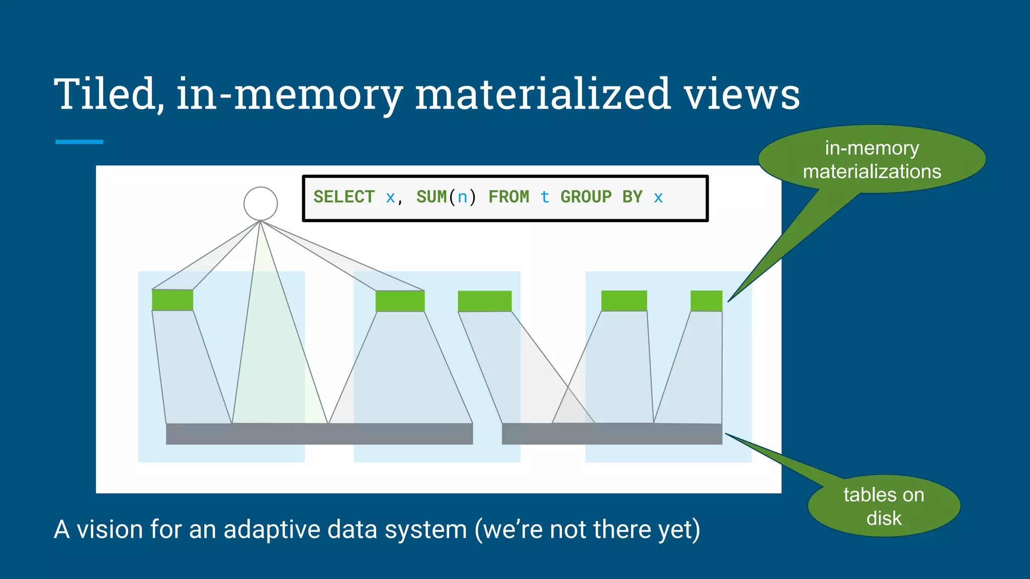
![Sketches
HyperLogLog is an algorithm that computes
approximate distinct count. It can estimate
cardinalities of 109
with a typical error rate of
2%, using 1.5 kB of memory. [3][4]
With 16 MB memory per machine we can
compute 10,000 combinations of attributes
each pass.
So, we’re down from 109
to 105
passes.
[3] Flajolet, Fusy, Gandouet, Meunier (2007). "Hyperloglog: The analysis of a near-optimal cardinality estimation algorithm"
[4] https://github.com/mrjgreen/HyperLogLog](https://image.slidesharecdn.com/calcite-data-eng-2017-171030074234/75/Don-t-optimize-my-queries-optimize-my-data-29-2048.jpg)
![Lattice after Query 1 + 2
Query 2
Query 1
Growing and evolving
lattices based on queries
sales
customers
product
product
class
sales
product
product
class
sales
customers
See: [CALCITE-1870] “Lattice suggester”](https://image.slidesharecdn.com/calcite-data-eng-2017-171030074234/75/Don-t-optimize-my-queries-optimize-my-data-36-2048.jpg)
![Thank you! Questions?
@julianhyde · @ApacheCalcite · http://apache.calcite.org
Resources
[CALCITE-1616] Data profiler
[CALCITE-1870] Lattice suggester
[CALCITE-1861] Spatial indexes
[CALCITE-1968] OpenGIS
[CALCITE-1991] Generated columns
Talk: “Data profiling with Apache Calcite” (Hadoop Summit, 2017)
Talk: “SQL on everything, in memory” (Strata, 2014)
Zhang, Qi, Stradling, Huang (2014). “Towards a Painless Index for Spatial Objects”
Harinarayan, Rajaraman, Ullman (1996). “Implementing data cubes efficiently”
Image credit
https://www.flickr.com/photos/defenceimages/6938469933/](https://image.slidesharecdn.com/calcite-data-eng-2017-171030074234/75/Don-t-optimize-my-queries-optimize-my-data-38-2048.jpg)


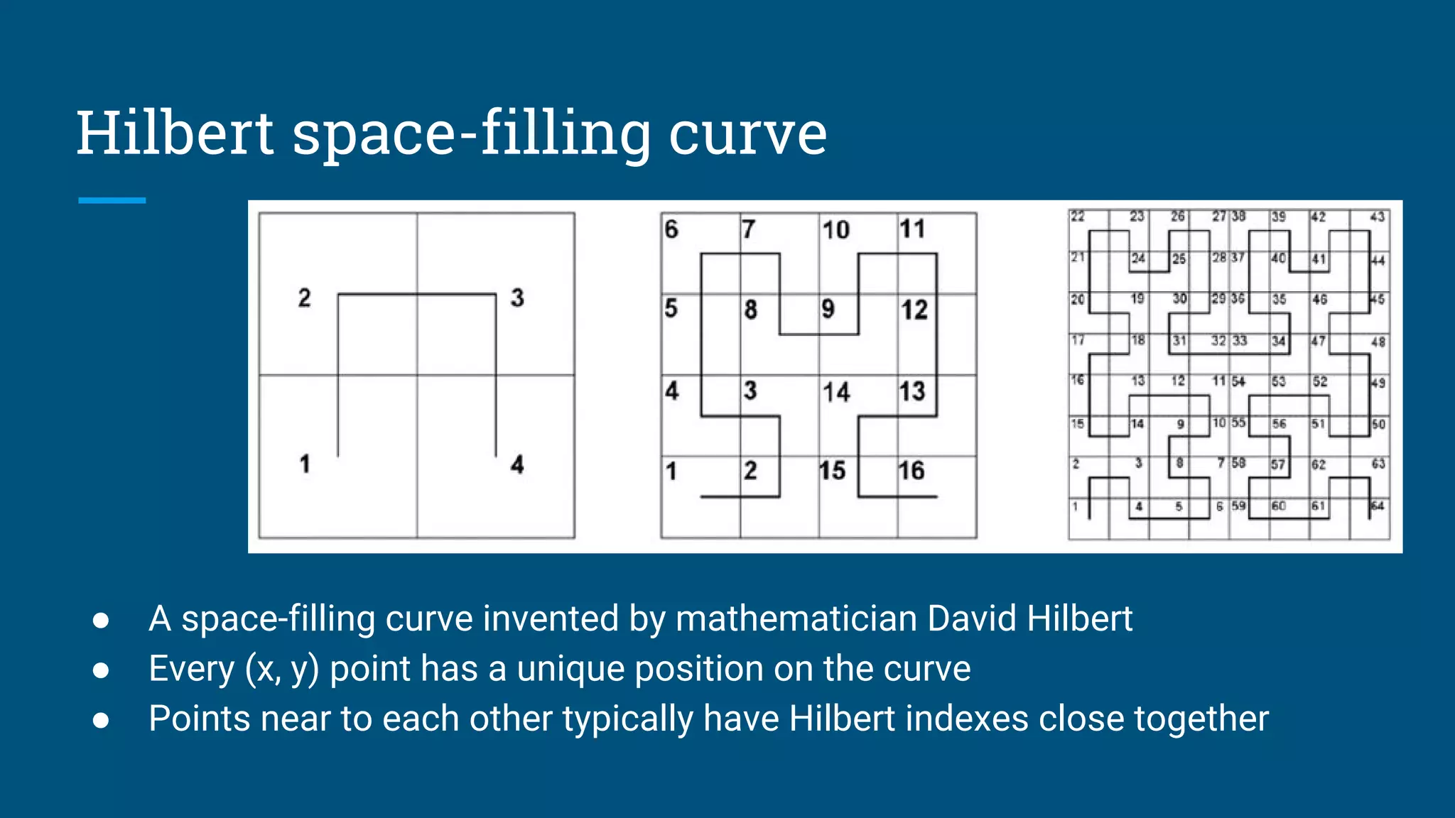
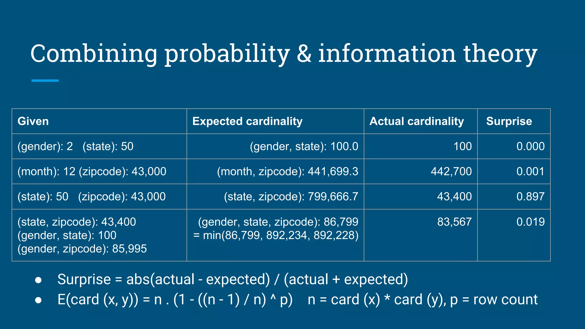
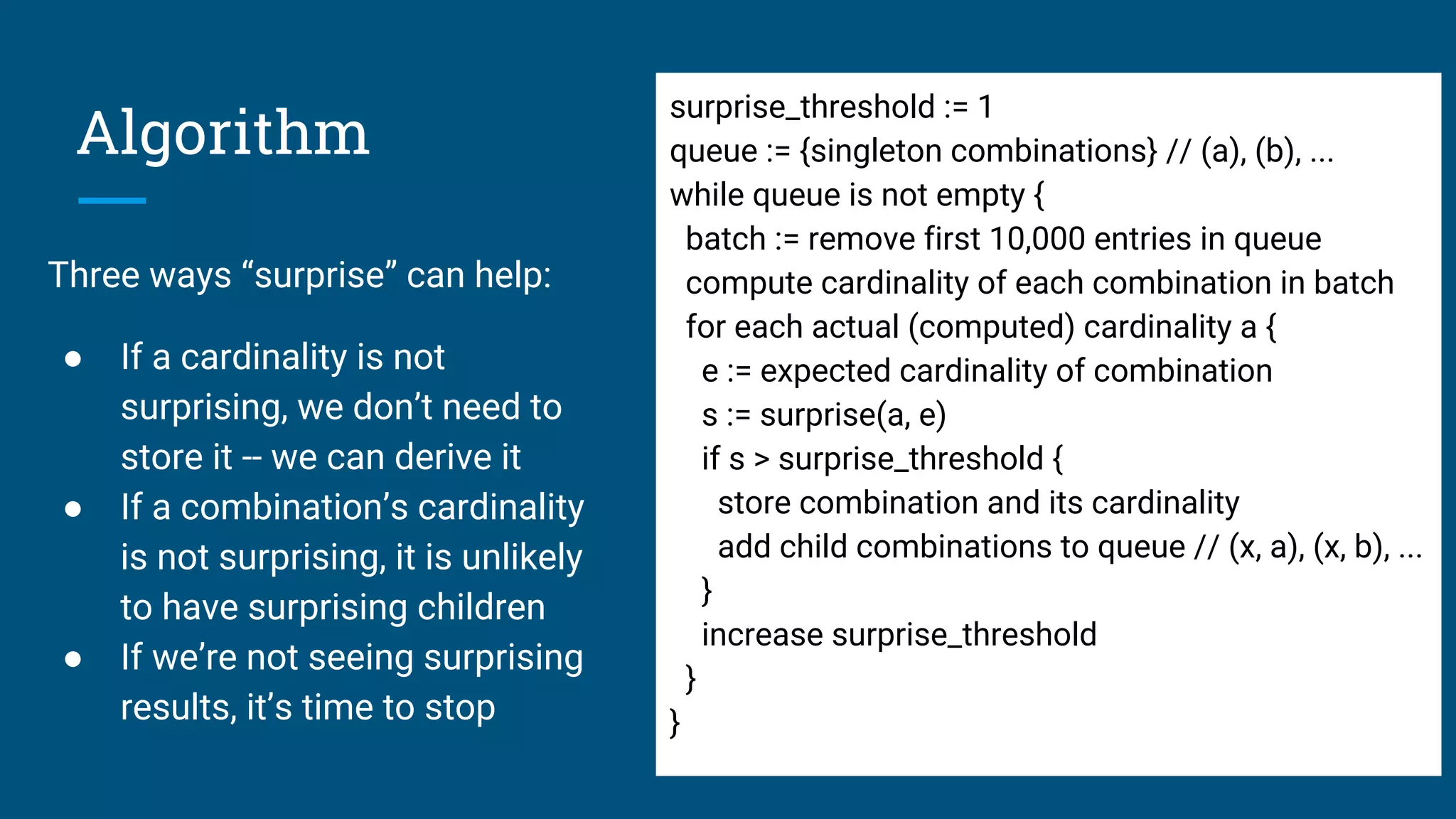
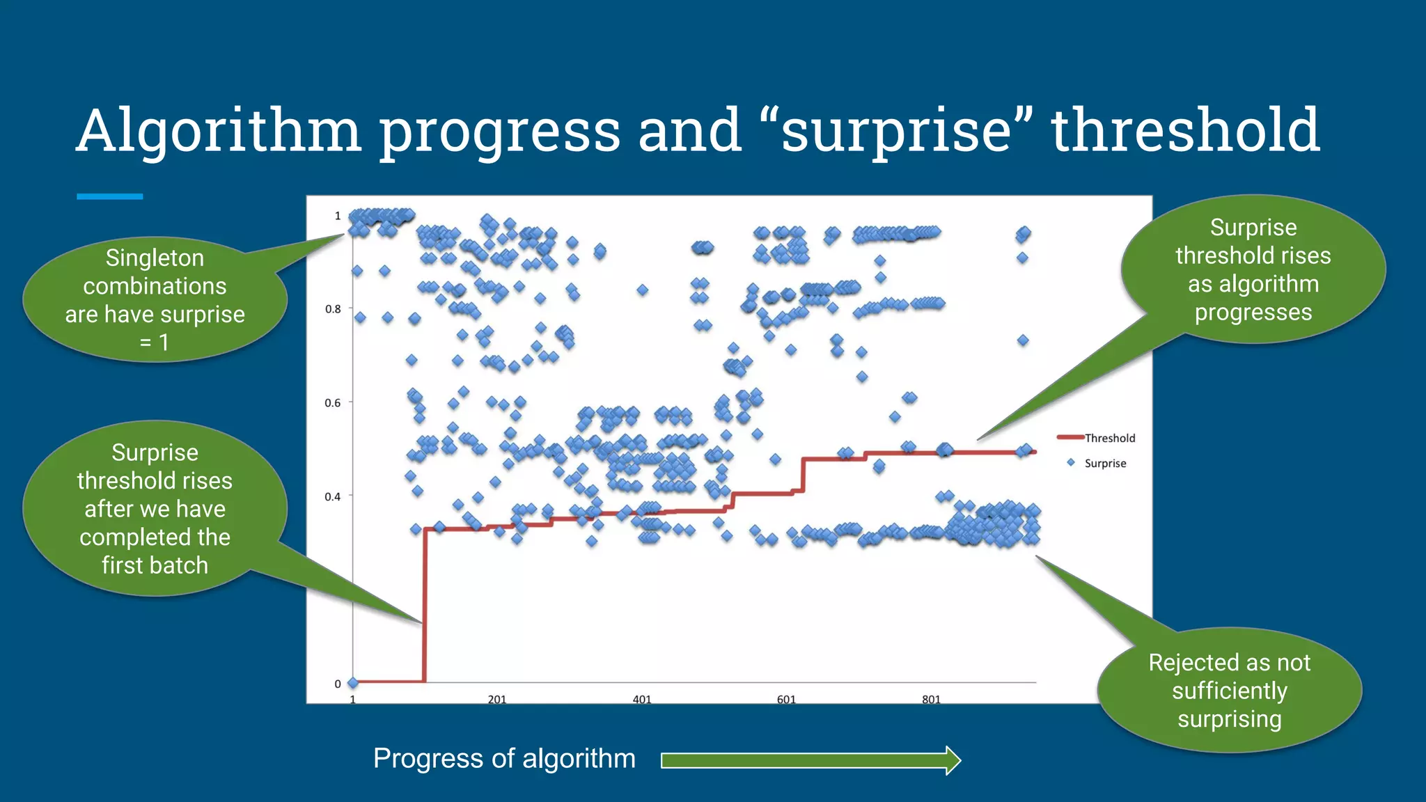
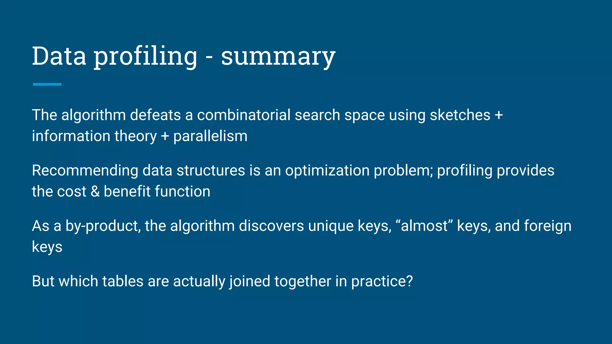
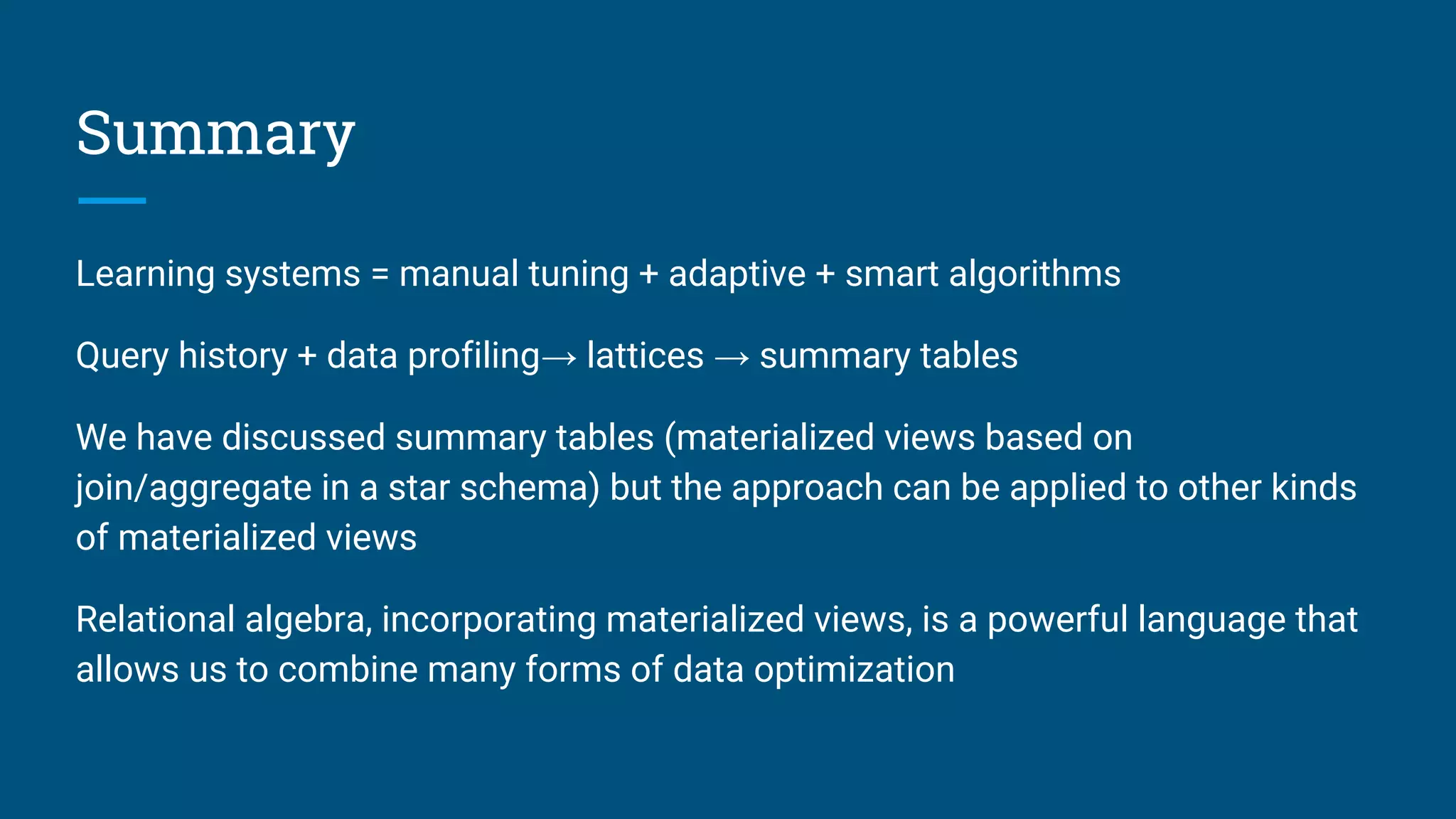
The document discusses strategies for optimizing data through materialized views and how data systems can learn to optimize themselves. It proposes an algorithm that uses sketches and information theory to profile data cardinalities and recommend materialized views. The algorithm aims to defeat the combinatorial search space by only considering combinations with "surprising" cardinalities. This profiling provides the cost and benefit information needed to optimize data structures. The document also discusses using query logs and statistics to infer relationships between tables and design summary tables through lattices.