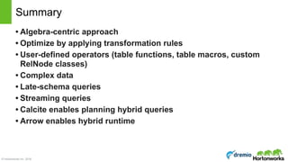
Download as PDF, PPTX

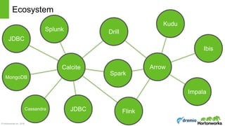
![© Hortonworks Inc. 2016
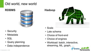
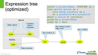
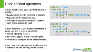
select d.name, COUNT(*) as c
from Emps as e
join Depts as d
on e.deptno = d.deptno
where e.age < 30
group by d.deptno
having count(*) > 5
order by c desc
Relational algebra
Scan [Emps] Scan [Depts]
Join [e.deptno
= d.deptno]
Filter [e.age < 30]
Aggregate [deptno, COUNT(*) AS c]
Filter [c > 5]
Project [name, c]
Sort [c DESC]
(Column names are simplified. They would usually
be ordinals, e.g. $0 is the first column of the left input.)](https://image.slidesharecdn.com/calcite-polyalgebra-dublin-2016-160414141449/85/Planning-with-Polyalgebra-Bringing-Together-Relational-Complex-and-Machine-Learning-Algebra-11-320.jpg)
![© Hortonworks Inc. 2016
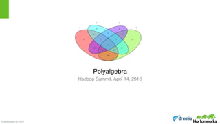
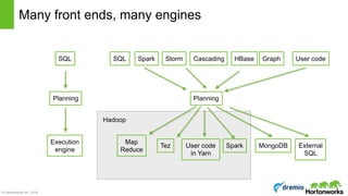
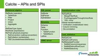
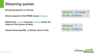
select * from (
select zipcode, state
from Emps
union all
select zipcode, state
from Customers)
where state in (‘CA’, ‘TX’)
Relational algebra - Union and sub-query
Scan [Emps] Scan [Customers]
Union [all]
Project [zipcode, state] Project [zipcode, state]
Filter [state IN (‘CA’, ‘TX’)]](https://image.slidesharecdn.com/calcite-polyalgebra-dublin-2016-160414141449/85/Planning-with-Polyalgebra-Bringing-Together-Relational-Complex-and-Machine-Learning-Algebra-12-320.jpg)
![© Hortonworks Inc. 2016
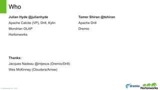
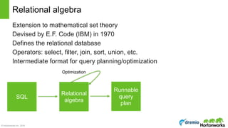
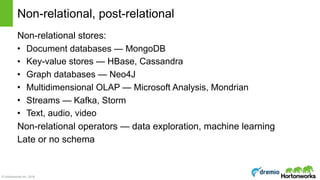
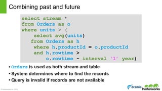
insert into Facts
values (‘Meaning of life’, 42),
(‘Clever as clever’, 6)
Relational algebra - Insert and Values
Insert [Facts]
Values [[‘Meaning of life’, 42],
[‘Clever as clever’, 6]]](https://image.slidesharecdn.com/calcite-polyalgebra-dublin-2016-160414141449/85/Planning-with-Polyalgebra-Bringing-Together-Relational-Complex-and-Machine-Learning-Algebra-13-320.jpg)

![© Hortonworks Inc. 2016
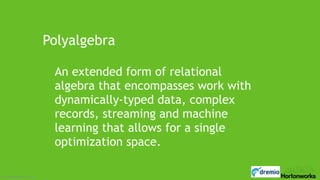
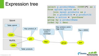
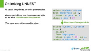
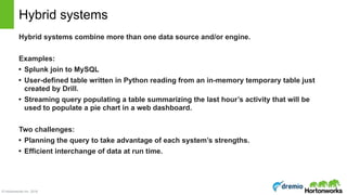
Calcite Planning Process
SQL
parse
tree
Planner
RelNode
Graph
Sql-to-Rel Converter
SqlNode !
RelNode + RexNode
• Node for each node in
Input Plan
• Each node is a Set of
alternate Sub Plans
• Set further divided into
Subsets: based on traits
like sortedness
1. Plan Graph
• Rule: specifies an Operator
sub-graph to match and
logic to generate equivalent
‘better’ sub-graph
• New and original sub-graph
both remain in contention
2. Rules
• RelNodes have Cost &
Cumulative Cost
3. Cost Model
- Used to plug in Schema,
cost formulas
- Filter selectivity
- Join selectivity
- NDV calculations
4. Metadata Providers
Rule Match Queue
- Add Rule matches to Queue
- Apply Rule match
transformations to plan graph
- Iterate for fixed iterations or until
cost doesn’t change
- Match importance based on
cost of RelNode and height
Best RelNode Graph
Translate to
runtime
Logical Plan
Based on “Volcano” & “Cascades” papers [G. Graefe]](https://image.slidesharecdn.com/calcite-polyalgebra-dublin-2016-160414141449/85/Planning-with-Polyalgebra-Bringing-Together-Relational-Complex-and-Machine-Learning-Algebra-18-320.jpg)
![© Hortonworks Inc. 2016
Algebra builder API
produces
final FrameworkConfig config;
final RelBuilder builder = RelBuilder.create(config);
final RelNode node = builder
.scan("EMP")
.aggregate(builder.groupKey("DEPTNO"),
builder.count(false, "C"),
builder.sum(false, "S", builder.field("SAL")))
.filter(
builder.call(SqlStdOperatorTable.GREATER_THAN,
builder.field("C"),
builder.literal(10)))
.build();
System.out.println(RelOptUtil.toString(node));
select deptno,
COUNT(*) as c,
sum(sal) as s
from Emp
having COUNT(*) > 10
LogicalFilter(condition=[>($1, 10)])
LogicalAggregate(group=[{7}], C=[COUNT()], S=[SUM($5)])
LogicalTableScan(table=[[scott, EMP]])
Equivalent SQL:](https://image.slidesharecdn.com/calcite-polyalgebra-dublin-2016-160414141449/85/Planning-with-Polyalgebra-Bringing-Together-Relational-Complex-and-Machine-Learning-Algebra-19-320.jpg)
![© Hortonworks Inc. 2016
Complex data, also known as nested or
document-oriented data. Typically, it can be
represented as JSON.
2 new operators are sufficient:
• UNNEST
• COLLECT aggregate function
Complex data employees: [
{
name: “Bob”,
age: 48,
pets: [
{name: “Jim”, type: “Dog”},
{name: “Frank”, type: “Cat”}
]
}, {
name: “Stacy",
age: 31,
starSign: ‘taurus’,
pets: [
{name: “Jack”, type: “Cat”}
]
}, {
name: “Ken”,
age: 23
}
]](https://image.slidesharecdn.com/calcite-polyalgebra-dublin-2016-160414141449/85/Planning-with-Polyalgebra-Bringing-Together-Relational-Complex-and-Machine-Learning-Algebra-21-320.jpg)
![© Hortonworks Inc. 2016
Flatten converts arrays of values to
separate rows:
• New record for each list item
• Empty lists removes record
Flatten is actually just syntactic sugar for
the UNNEST relational operator:
UNNEST and Flatten
name age pets
Bob 48 [{name: Jim, type: dog},
{name:Frank, type: dog}]
Stacy 31 [{name: Jack, type: cat}]
Ken 23 []
name age pet
Bob 48 {name: Jim, type: dog}
Bob 48 {name: Frank, type: dog}
Stacy 31 {name: Jack, type: cat}
select e.name, e.age,
flatten(e.pet)
from Employees as e
select e.name, e.age,
row(a.name, a.type)
from Employees as e,
unnest e.addresses as a](https://image.slidesharecdn.com/calcite-polyalgebra-dublin-2016-160414141449/85/Planning-with-Polyalgebra-Bringing-Together-Relational-Complex-and-Machine-Learning-Algebra-22-320.jpg)
![© Hortonworks Inc. 2016
Optimizing UNNEST (2)
We can also optimize projects.
If table is stored in a column-oriented file
format, this reduces disk reads significantly.
• Array wildcard projection through flatten
• Non-flattened column inclusion
select e.name,
flatten(pets).name
from Employees as e
scan(name, age, pets)
flatten(pets) as pet
project(name, pet.name)
scan(name, pets[*].name)
flatten(pets) as pet
scan(name, age, pets)
flatten(pets as pet)
project(name, pets[*].name)
Original Plan Project through Flatten
Project into scan
(less data read)
ProjectFlattenTransposeRule ProjectScanRule](https://image.slidesharecdn.com/calcite-polyalgebra-dublin-2016-160414141449/85/Planning-with-Polyalgebra-Bringing-Together-Relational-Complex-and-Machine-Learning-Algebra-24-320.jpg)
![© Hortonworks Inc. 2016
Evolution:
• Oracle: Schema before write, strongly typed SQL (like Java)
• Hive: Schema before query, strongly typed SQL
• Drill: Schema on data, weakly typed SQL (like JavaScript)
Late schema
name age starSign pets
Bob 48 [{name: Jim, type: dog},
{name:Frank, type: dog}]
Stacy 31 Taurus [{name: Jack, type: cat}]
Ken 23 []
name age pets
Ken 23 []
select *
from Employees
select *
from Employees
where age < 30
no starSign column!](https://image.slidesharecdn.com/calcite-polyalgebra-dublin-2016-160414141449/85/Planning-with-Polyalgebra-Bringing-Together-Relational-Complex-and-Machine-Learning-Algebra-25-320.jpg)
![© Hortonworks Inc. 2016
Expanding *
• Early schema databases expand * at planning time, based on schema
• Drill expands * during query execution
• Each operator needs to be able to propagate column names/types as well as data
Internally, Drill is strongly typed
• Strong typing means efficient code
• JavaScript engines do this too
• Infer type for each batch of records
• Throw away generated code if a column changes type in the next batch of records
Implementing schema-on-data
select e.name
from Employees
where e.age < 30
select e._map[“name”] as name
from Employees
where cast(e._map[“age”] as integer) < 30](https://image.slidesharecdn.com/calcite-polyalgebra-dublin-2016-160414141449/85/Planning-with-Polyalgebra-Bringing-Together-Relational-Complex-and-Machine-Learning-Algebra-26-320.jpg)
![© Hortonworks Inc. 2016
Views
Scan [Emps]
Join [$0, $5]
Project [$0, $1, $2, $3]
Filter [age >= 50]
Aggregate [deptno, min(salary)]
Scan [Managers]
Aggregate [manager]
Scan [Emps]
select deptno, min(salary)
from Managers
where age >= 50
group by deptno
create view Managers as
select *
from Emps as e
where exists (
select *
from Emps as underling
where underling.manager = e.id)](https://image.slidesharecdn.com/calcite-polyalgebra-dublin-2016-160414141449/85/Planning-with-Polyalgebra-Bringing-Together-Relational-Complex-and-Machine-Learning-Algebra-28-320.jpg)
![© Hortonworks Inc. 2016
Views (after expansion)
select deptno, min(salary)
from Managers
where age >= 50
group by deptno
create view Managers as
select *
from Emps as e
where exists (
select *
from Emps as underling
where underling.manager = e.id)
Scan [Emps] Aggregate [manager]
Join [$0, $5]
Project [$0, $1, $2, $3]
Filter [age >= 50]
Aggregate [deptno, min(salary)]
Scan [Emps]](https://image.slidesharecdn.com/calcite-polyalgebra-dublin-2016-160414141449/85/Planning-with-Polyalgebra-Bringing-Together-Relational-Complex-and-Machine-Learning-Algebra-29-320.jpg)
![© Hortonworks Inc. 2016
Views (after pushing down filter)
select deptno, min(salary)
from Managers
where age >= 50
group by deptno
create view Managers as
select *
from Emps as e
where exists (
select *
from Emps as underling
where underling.manager = e.id) Scan [Emps]
Scan [Emps]
Join [$0, $5]
Project [$0, $1, $2, $3]
Filter [age >= 50]
Aggregate [deptno, min(salary)]](https://image.slidesharecdn.com/calcite-polyalgebra-dublin-2016-160414141449/85/Planning-with-Polyalgebra-Bringing-Together-Relational-Complex-and-Machine-Learning-Algebra-30-320.jpg)
![© Hortonworks Inc. 2016
Materialized view
create materialized view
EmpSummary as
select deptno,
gender,
count(*) as c,
sum(sal)
from Emps
group by deptno, gender
select count(*) as c
from Emps
where deptno = 10
and gender = ‘M’
Scan [Emps]
Aggregate [deptno, gender,
COUNT(*), SUM(sal)]
Scan [EmpSummary] =
Scan [Emps]
Filter [deptno = 10 AND gender = ‘M’]
Aggregate [COUNT(*)]](https://image.slidesharecdn.com/calcite-polyalgebra-dublin-2016-160414141449/85/Planning-with-Polyalgebra-Bringing-Together-Relational-Complex-and-Machine-Learning-Algebra-31-320.jpg)
![© Hortonworks Inc. 2016
Materialized view, step 2: Rewrite query to match
create materialized view
EmpSummary as
select deptno,
gender,
count(*) as c,
sum(sal)
from Emps
group by deptno, gender
select count(*) as c
from Emps
where deptno = 10
and gender = ‘M’
Scan [Emps]
Aggregate [deptno, gender,
COUNT(*), SUM(sal)]
Scan [EmpSummary] =
Scan [Emps]
Filter [deptno = 10 AND gender = ‘M’]
Aggregate [deptno, gender,
COUNT(*) AS c, SUM(sal) AS s]
Project [c]](https://image.slidesharecdn.com/calcite-polyalgebra-dublin-2016-160414141449/85/Planning-with-Polyalgebra-Bringing-Together-Relational-Complex-and-Machine-Learning-Algebra-32-320.jpg)
![© Hortonworks Inc. 2016
Materialized view, step 3: substitute table
create materialized view
EmpSummary as
select deptno,
gender,
count(*) as c,
sum(sal)
from Emps
group by deptno, gender
select count(*) as c
from Emps
where deptno = 10
and gender = ‘M’
Scan [Emps]
Aggregate [deptno, gender,
COUNT(*), SUM(sal)]
Scan [EmpSummary] =
Filter [deptno = 10 AND gender = ‘M’]
Project [c]
Scan [EmpSummary]](https://image.slidesharecdn.com/calcite-polyalgebra-dublin-2016-160414141449/85/Planning-with-Polyalgebra-Bringing-Together-Relational-Complex-and-Machine-Learning-Algebra-33-320.jpg)
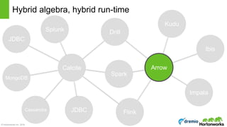

The document discusses the concepts of poly algebra and extended relational algebra within the context of data processing and analysis, emphasizing the importance of optimization in handling various data types and query processing. It highlights the Apache Calcite framework and its integration with different data engines, non-relational databases, and streaming queries for efficient data management. Additionally, it describes advancements in hybrid systems and the Arrow project aimed at enhancing in-memory analytics performance.