Download to read offline
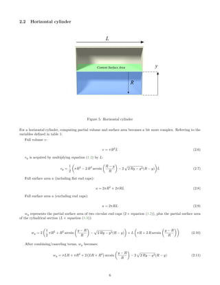
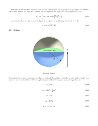
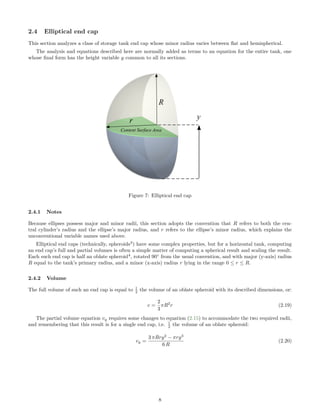

This document provides equations for calculating volumes, surface areas, and other metrics for common storage container geometries like cylinders, spheres, and elliptical end caps. It defines key variables and presents equations in increasing order of complexity, from simple circles to horizontal cylinders to more complex elliptical end caps. The goal is to create accurate summaries and sensor height to volume tables to model real storage tanks.