


![6.3. GEOGRAPHICAL DISTRIBUTION 79
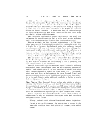
pure platinum wire whose resistance is a function of temperature. It is calibrated
at fixed points between the triple point of equilibrium hydrogen at 13.8033 K
and the freezing point of silver at 961.78 K, including the triple point of water
at 0.060◦
C, the melting point of Gallium at 29.7646◦
C, and the freezing point
of Indium at 156.5985◦
C (Preston-Thomas, 1990). The triple point of water is
the temperature at which ice, water, and water vapor are in equilibrium. The
temperature scale in kelvin T is related to the temperature scale in degrees
Celsius t/◦
C by:
t [◦
C] = T [K] − 273.15 (6.5)
The practical temperature scale was revised in 1887, 1927, 1948, 1968, and
1990 as more accurate determinations of absolute temperature became accepted.
The most recent scale is the International Temperature Scale of 1990 (its-90).
It differs slightly from the International Practical Temperature Scale of 1968
ipts-68. At 0◦
C they are the same, and above 0◦
C its-90 is slightly cooler.
t90 − t68 = −0.002 at 10◦
C, −0.005 at 20◦
C, −0.007 at 30◦
C and −0.010 at
40◦
C.
Notice that while oceanographers use thermometers calibrated with an ac-
curacy of a millidegree, which is 0.001◦
C, the temperature scale itself has un-
certainties of a few millidegrees.
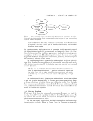
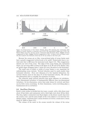
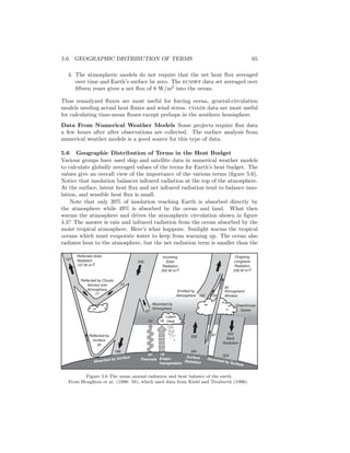
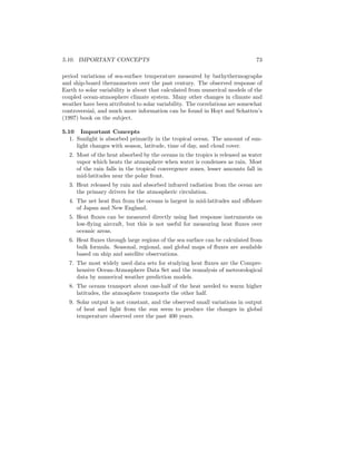
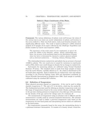
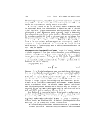
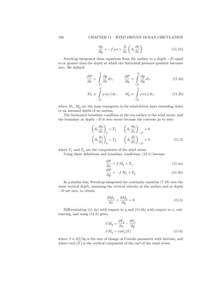
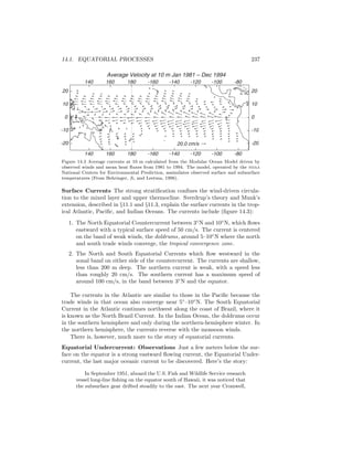
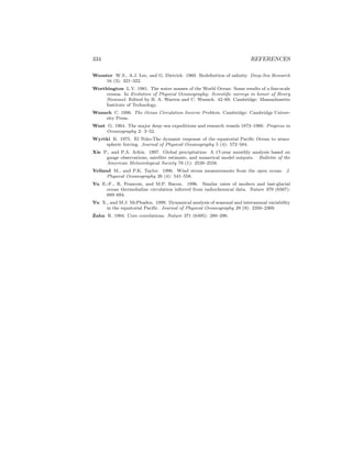
6.3 Geographical Distribution of Surface Temperature and Salinity
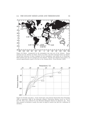
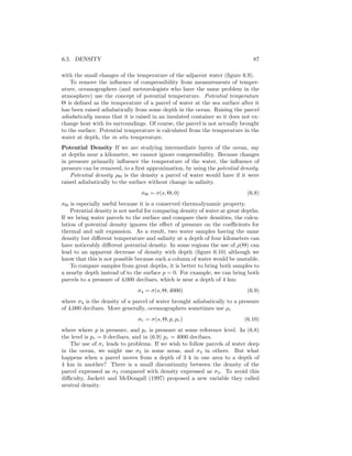
The distribution of temperature at the sea surface tends to be zonal, that is, it is
independent of longitude (figure 6.2). Warmest water is near the equator, coldest
water is near the poles. The deviations from zonal are small. Equatorward of
40◦
, cooler waters tend to be on the eastern side of the basin. North of this
latitude, cooler waters tend to be on the western side.
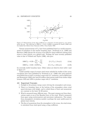
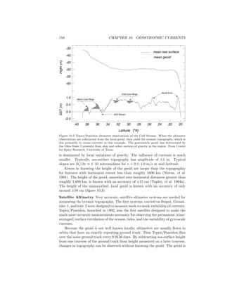
The anomalies of sea-surface temperature, the deviation from a long term
average, are small, less than 1.5◦
C except in the equatorial Pacific where the
deviations can be 3◦
C (figure 6.3: top).
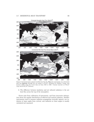
The annual range of surface temperature is highest at mid-latitudes, espe-
cially on the western side of the ocean (figure 6.3: bottom). In the west, cold air
blows off the continents in winter and cools the ocean. The cooling dominates
the heat budget. In the tropics the temperature range is mostly less than 2◦
C.
The distribution of sea-surface salinity also tends to be zonal. The saltiest
waters are at mid-latitudes where evaporation is high. Less salty waters are near
the equator where rain freshens the surface water, and at high latitudes where
melted sea ice freshens the surface waters (figure 6.4). The zonal (east-west)
average of salinity shows a close correlation between salinity and evaporation
minus precipitation plus river input (figure 6.5).
Because many large rivers drain into the Atlantic and the Arctic Sea, why
is the Atlantic saltier than the Pacific? Broecker (1997) showed that 0.32 Sv of
the water evaporated from the Atlantic does not fall as rain on land. Instead,
it is carried by winds into the Pacific (figure 6.6). Broecker points out that the
quantity is small, equivalent to a little more than the flow in the Amazon River,](https://image.slidesharecdn.com/introductiontophysicaloceanography-130610201256-phpapp02/85/Introduction-to-physical-oceanography-87-320.jpg)

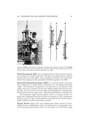
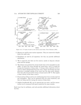
![6.6. MEASUREMENT OF TEMPERATURE 93
4.0
T T11 3.7-T11
6.0
5.0
4.0
3.0
2.0
1.0
0
0
Local Mean Temperature Difference [K]
3.02.01.0
LocalMaximumDifference
10
5
0
270 275 280 285 290 295
LocalStandardDeviation
Local Mean Temperature [K]
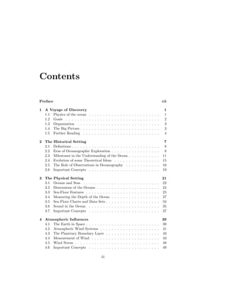
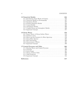
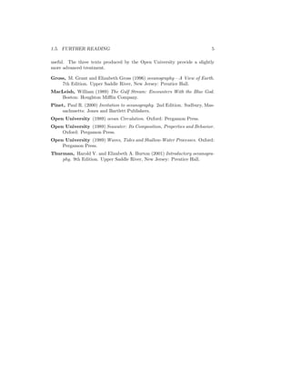
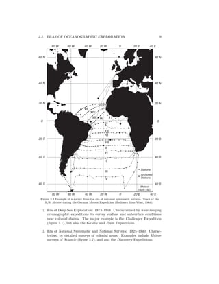
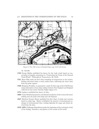
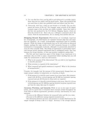
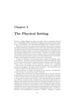
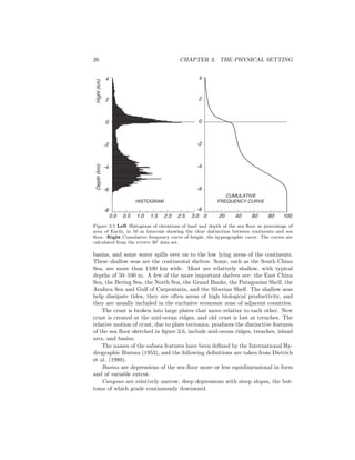
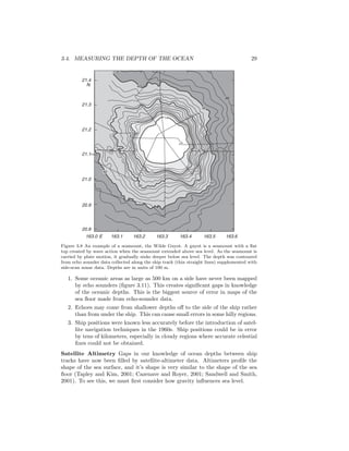
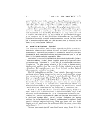
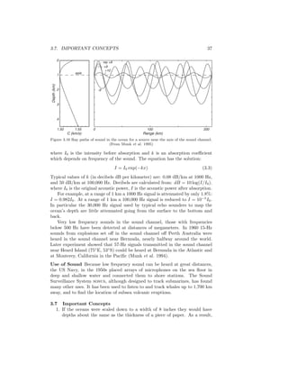
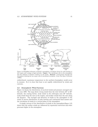
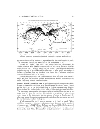
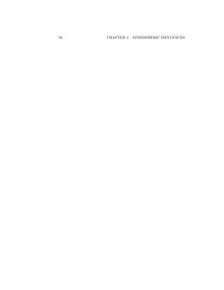
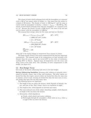
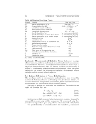
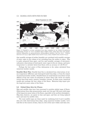
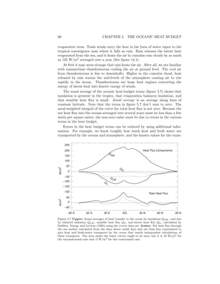
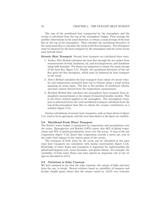
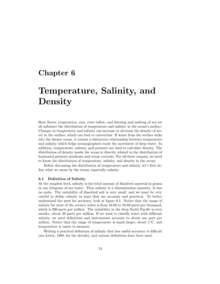
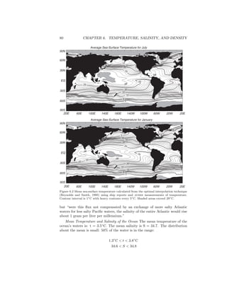
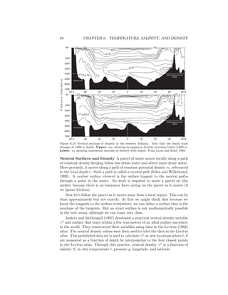
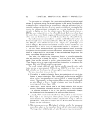
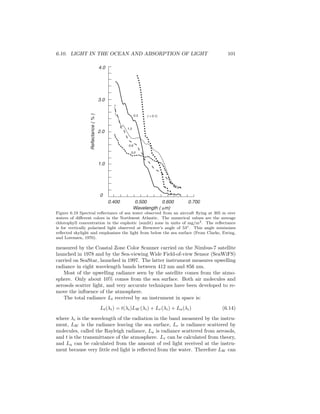
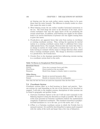
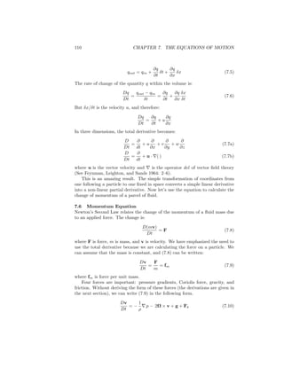
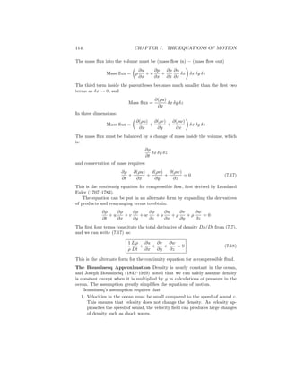
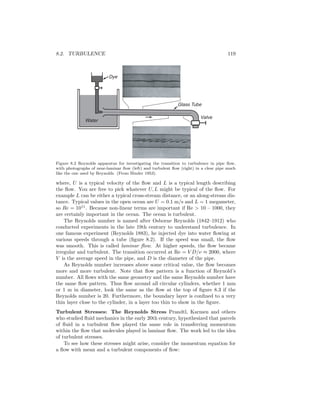
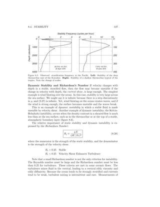
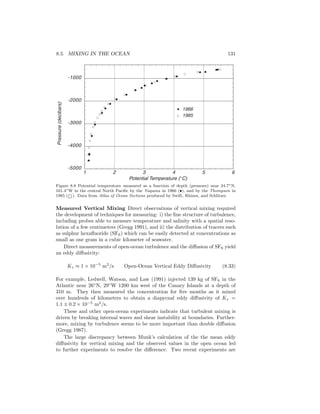
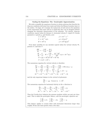
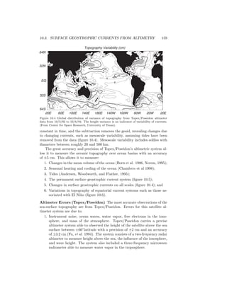
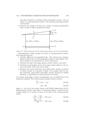
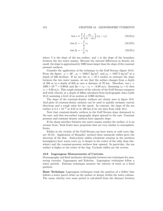
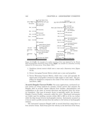
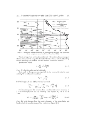
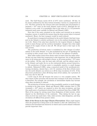
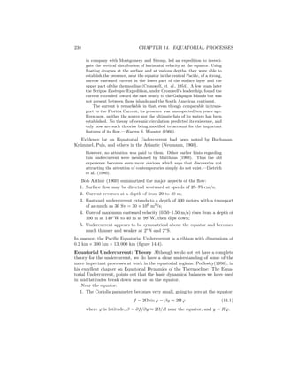
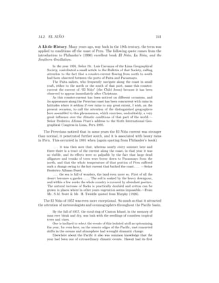
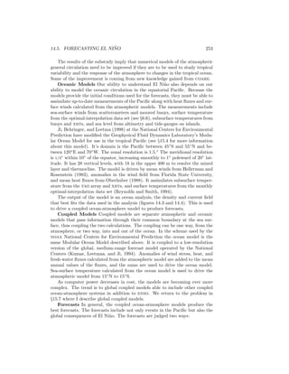
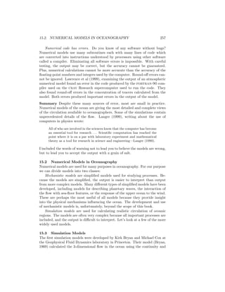
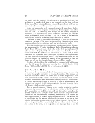
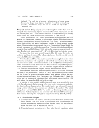
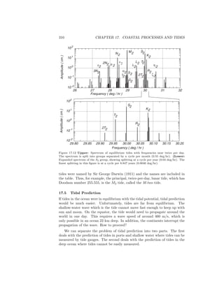
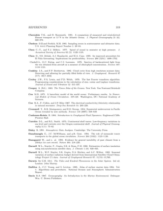
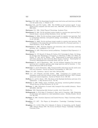
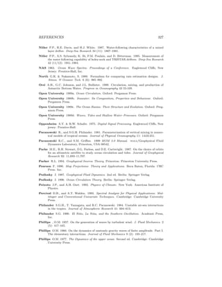
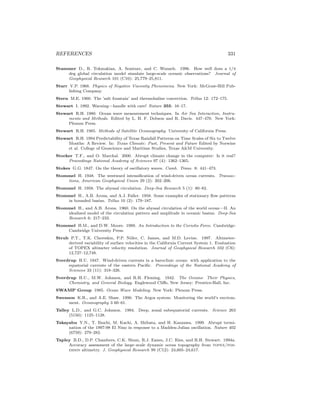
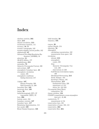
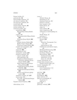
Figure 6.12 The influence of clouds on infrared observations. Left: The standard deviation
of the radiance from small, partly cloudy areas each containing 64 pixels. The feet of
the arch-like distribution of points are the sea-surface and cloud-top temperatures. (After
Coakley and Bretherton (1982). Right: The maximum difference between local values of
T11 − T3.7 and the local mean values of the same quantity. Values inside the dashed box
indicate cloud-free pixels. T11 and T3.7 are the apparent temperatures at 11.0 and 3.7 µm
(data from K. Kelly). ¿From Stewart (1985).
below the sea surface. They can differ by several degrees when winds are
light (Emery and Schussel, 1989). This error is greatly reduced whan
avhrr data are used to interpolate between ship measurements of surface
temperature.
Maps of temperature processed from Local Area Coverage of cloud-free re-
gions show variations of temperature with a precision of 0.1◦
C. These maps
are useful for observing local phenomena including patterns produced by local
currents. Figure 10.16 shows such patterns off the California coast.
Global maps are made by the U.S. Naval Oceanographic Office, which re-
ceives the global avhrr data directly from noaa’s National Environmental
Satellite, Data and Information Service in near-real time each day. The data
are carefully processed to remove the influence of clouds, water vapor, aerosols,
and other sources of error. Data are then used to produce global maps between
±70◦
with an accuracy of ±0.6◦
C (May et al 1998). The maps of sea-surface
temperature are sent to the U.S. Navy and to noaa’s National Centers for En-
vironmental Prediction. In addition, the office produces daily 100-km global
and 14-km regional maps of temperature.
Global Maps of Sea-Surface Temperature Global, monthly maps of sur-
face temperature are produced by the National Centers for Environmental Pre-
diction using Reynolds’ (1988, 1993, 1994) optimal-interpolation method. The
technique blends ship and buoy measurements of sea-surface temperature with
avhrr data processed by the Naval Oceanographic Office in 1◦
areas for a
month. Essentially, avhrr data are interpolated between buoy and ship re-
ports using previous information about the temperature field. Overall accuracy
ranges from approximately ±0.3◦
C in the tropics to ±0.5◦
C near western
boundary currents in the northern hemisphere where temperature gradients are](https://image.slidesharecdn.com/introductiontophysicaloceanography-130610201256-phpapp02/85/Introduction-to-physical-oceanography-101-320.jpg)


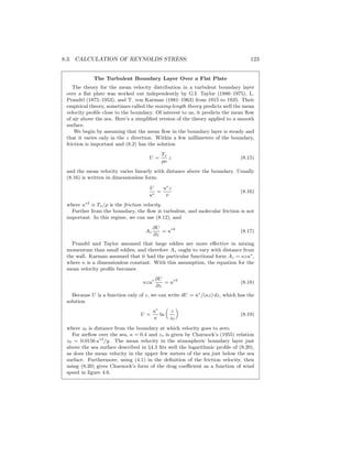
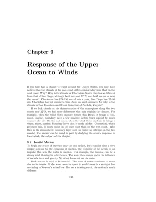
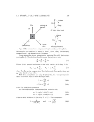
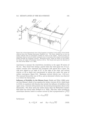
![9.2. EKMAN LAYER AT THE SEA SURFACE 141
where ρair is the density of air, CD is the drag coefficient, and U10 is the wind
speed at 10 m above the sea. Ekman turned to the literature to obtain values
for V0 as a function of wind speed. He found:
V0 =
0.0127
sin |ϕ|
U10, |ϕ| ≥ 10 (9.14)
With this information, he could then calculate the velocity as a function of
depth knowing the wind speed U10 and wind direction.
Ekman Layer Depth The thickness of the Ekman layer is arbitrary because
the Ekman currents decrease exponentially with depth. Ekman proposed that
the thickness be the depth DE at which the current velocity is opposite the
velocity at the surface, which occurs at a depth DE = π/a, and the Ekman
layer depth is:
DE =
2π2 Az
f
(9.15)
Using (9.13) in (9.10), dividing by U10, and using (9.14) and (9.15) gives:
DE =
7.6
sin |ϕ|
U10 (9.16)
in SI units. Wind in meters per second gives depth in meters. The constant in
(9.16) is based on ρw = 1027 kg/m3
, ρair = 1.25 kg/m3
, and Ekman’s value of
CD = 2.6 × 10⁻³
for the drag coefficient.
Using (9.16) with typical winds, the depth of the Ekman layer varies from
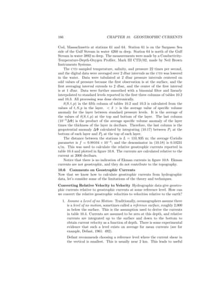
about 45 to 300 meters (Table 9.3), and the velocity of the surface current varies
from 2.5% to 1.1% of the wind speed depending on latitude.
Table 9.3 Typical Ekman Depths
Latitude
U10 [m/s] 15◦
45◦
5 75 m 45 m
10 150 m 90 m
20 300 m 180 m
The Ekman Number: Coriolis and Frictional Forces The depth of the
Ekman layer is closely related to the depth at which frictional force is equal to
the Coriolis force in the momentum equation (9.9). The Coriolis force is fu,
and the frictional force is Az∂2
U/∂z2
. The ratio of the forces, which is non
dimensional, is called the Ekman Number Ez:
Ez =
Friction Force
Coriolis Force
=
Az
∂2
u
∂z2
fu
=
Az
u
d2
fu](https://image.slidesharecdn.com/introductiontophysicaloceanography-130610201256-phpapp02/85/Introduction-to-physical-oceanography-149-320.jpg)
![142 CHAPTER 9. RESPONSE OF THE UPPER OCEAN TO WINDS
Ez =
Az
f d2
(9.17)
where we have approximated the terms using typical velocities u, and typical
depths d. The subscript z is needed because the ocean is stratified and mixing
in the vertical is much less than mixing in the horizontal. Note that as depth
increases, friction becomes small, and eventually, only the Coriolis force remains.
Solving (9.17) for d gives
d =
Az
fEz
(9.18)
which agrees with the functional form (9.15) proposed by Ekman. Equating
(9.18) and (9.15) requires Ez = 1/(2π2
) = 0.05 at the Ekman depth. Thus Ek-
man chose a depth at which frictional forces are much smaller than the Coriolis
force.
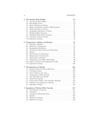
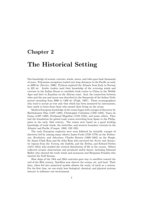
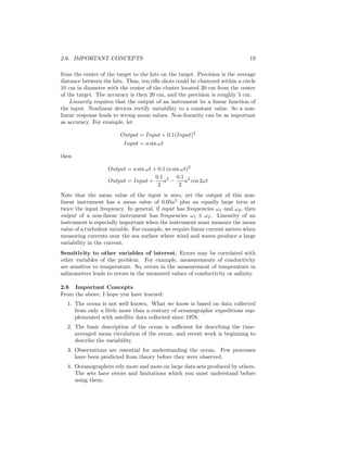
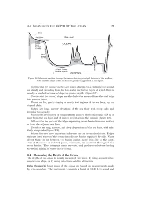
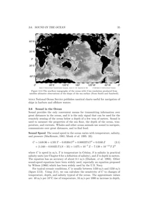
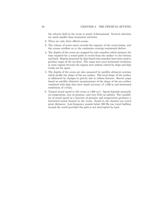
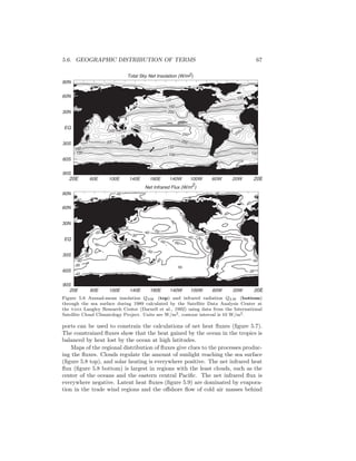
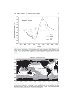
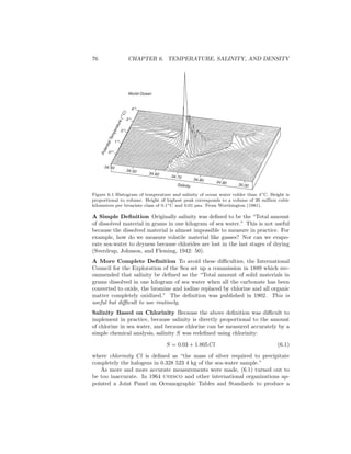
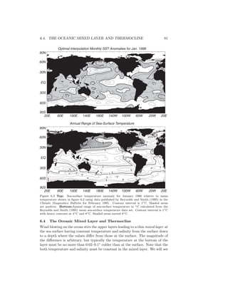
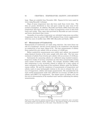
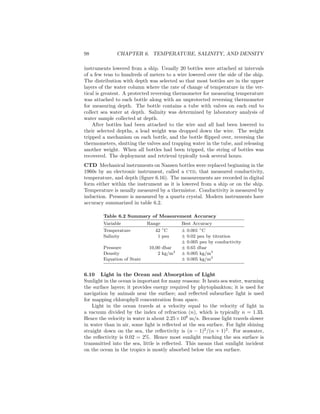
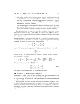
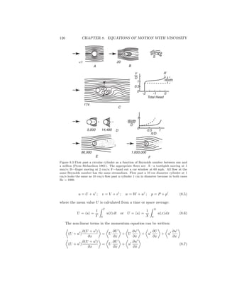
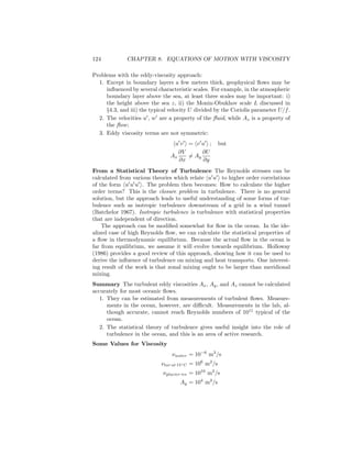
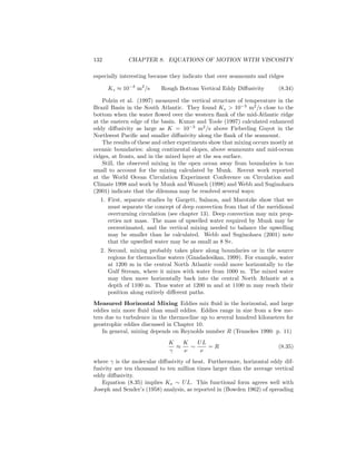
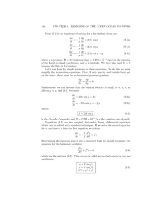
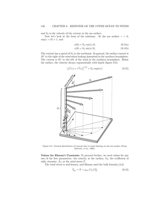
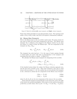
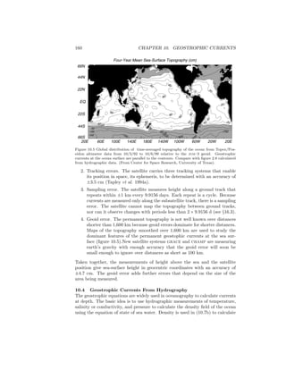
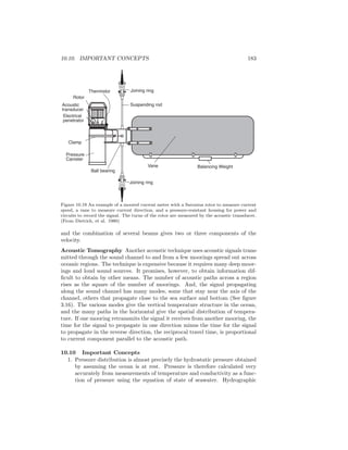
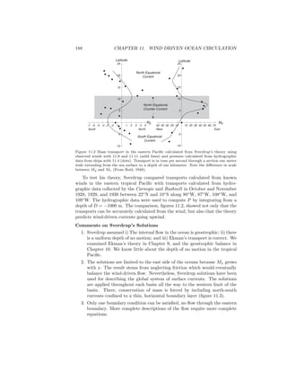
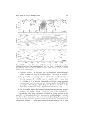
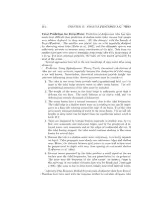
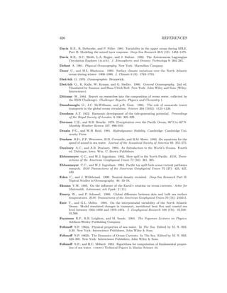
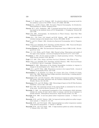
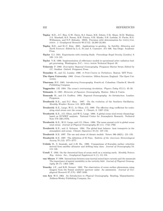
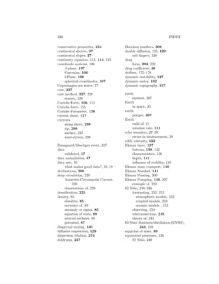
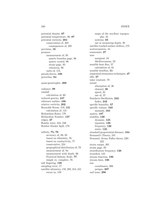
Bottom Ekman Layer The Ekman layer at the bottom of the ocean and
the atmosphere differs from the layer at the ocean surface. The solution for a
bottom layer below a fluid with velocity U in the x-direction is:
u = U[1 − exp(−az) cos az] (9.19a)
v = U exp(−az) sin az (9.19b)
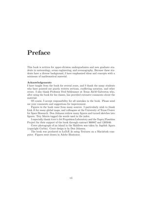
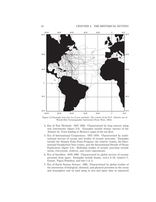
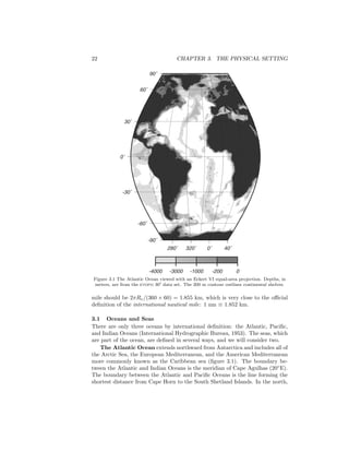
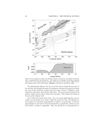
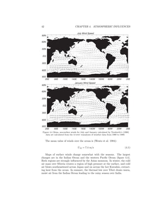
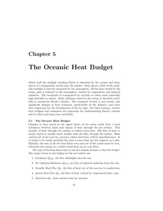
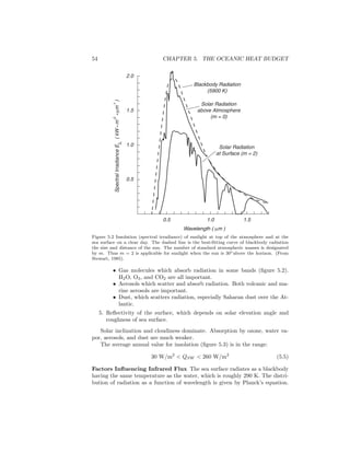
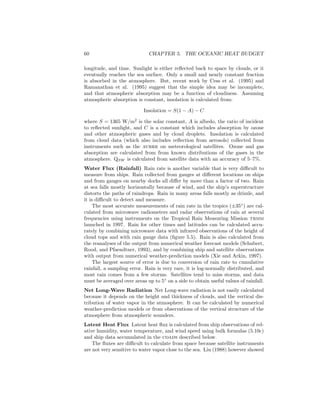
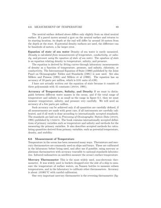
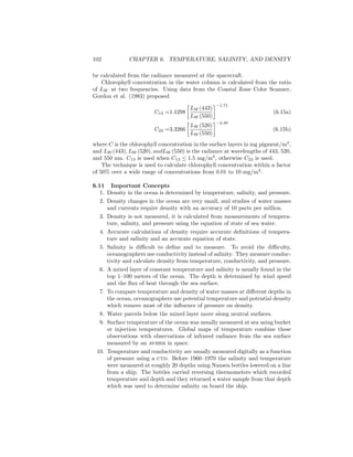
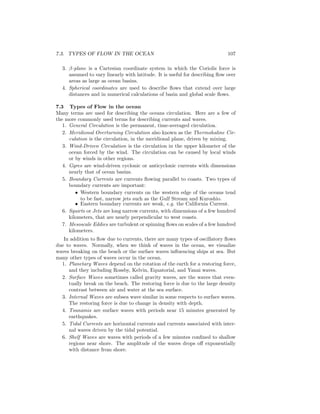
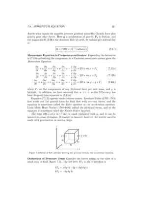
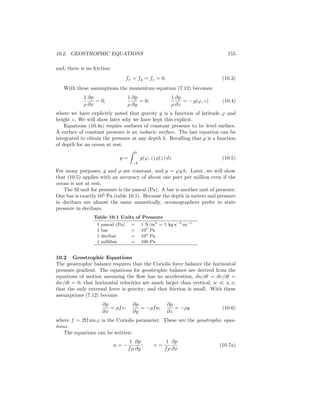
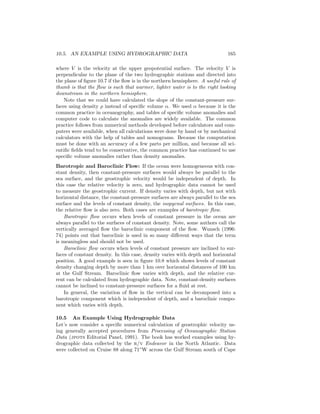
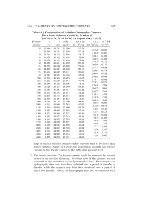
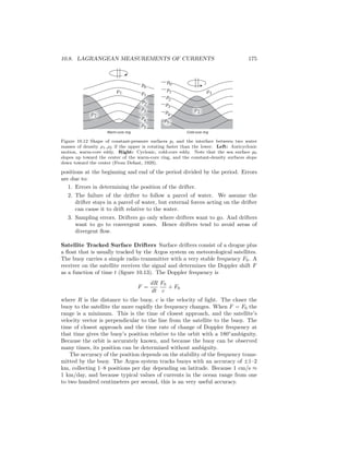
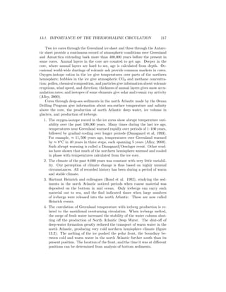
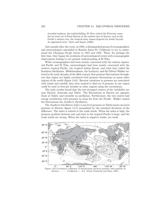
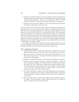
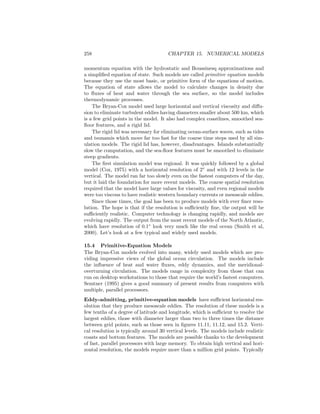
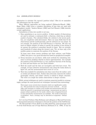
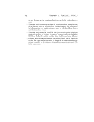
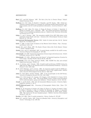
The velocity goes to zero at the boundary, u = v = 0 at z = 0. The direction
of the flow close to the boundary is 45◦
to the left of the flow U outside the
boundary layer in the northern hemisphere, and the direction of the flow rotates
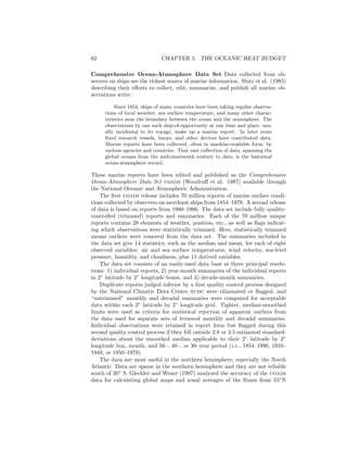
with distance above the boundary (figure 9.4). The direction of rotation is anti-
cyclonic with distance above the bottom.
Winds above the planetary boundary layer are perpendicular to the pressure
gradient in the atmosphere and parallel to lines of constant surface pressure.
4
0 4 8 12
u (m/s)
v(m/s)
200 300
600
1000
30 305
610
910
100
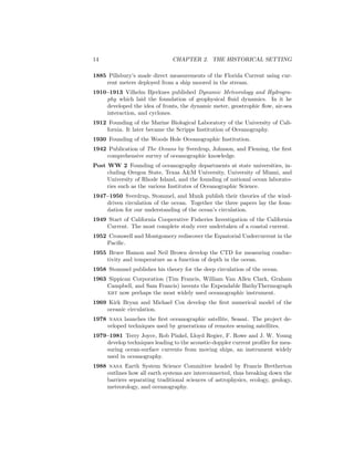
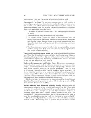
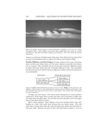
Figure 9.4 Ekman layer for the lowest kilometer in the atmosphere (solid line), together
with wind velocity measured by Dobson (1914) - - - . The numbers give height above the
surface in meters. The boundary layer at the bottom of the ocean has a similar shape. (From
Houghton, 1977).](https://image.slidesharecdn.com/introductiontophysicaloceanography-130610201256-phpapp02/85/Introduction-to-physical-oceanography-150-320.jpg)
![9.4. APPLICATION OF EKMAN THEORY 149
2. Currents along the eastern side of oceans at mid-latitudes tend to bring
colder water from higher latitudes.
3. The marine boundary layer in the atmosphere, that layer of moist air
above the sea, is only a few hundred meters thick in the eastern Pacific
near California. It is over a kilometer thick near Asia.
All these processes are reversed offshore of east coasts, leading to warm water
close to shore, thick atmospheric boundary layers, and frequent convective rain.
Thus Norfolk is much different that San Francisco due to upwelling and the
direction of the coastal currents.
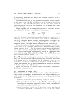
Ekman Pumping The horizontal variability of the wind blowing on the sea
surface leads to horizontal variability of the Ekman transports. Because mass
must be conserved, the spatial variability of the transports must lead to vertical
velocities at the top of the Ekman layer. To calculate this velocity, we first
integrate the continuity equation (7.19) in the vertical:
ρ
0
−d
∂u
∂x
+
∂v
∂y
+
∂w
∂z
dz = 0
∂
∂x
0
−d
ρ u dz +
∂
∂y
0
−d
ρ v dz = −ρ
0
−d
∂w
∂z
dz
∂MEx
∂x
+
∂MEy
∂y
= −ρ [w(0) − w(−d)] (9.28)
By definition, the Ekman velocities approach zero at the base of the Ekman
layer, and the vertical velocity at the base of the layer wE(−d) due to divergence
of the Ekman flow must be zero. Therefore:
∂MEx
∂x
+
∂MEy
∂y
= −ρ wE(0) (9.29a)
∇H · ME = −ρ wE(0) (9.29b)
Where ME is the vector mass transport due to Ekman flow in the upper bound-
ary layer of the ocean, and ∇H is the horizontal divergence operator. (9.29)
states that the horizontal divergence of the Ekman transports leads to a verti-
cal velocity in the upper boundary layer of the ocean, a process called Ekman
Pumping.
If we use the Ekman mass transports (9.26) in (9.29) we can relate Ekman
pumping to the wind stress.
wE(0) = −
1
ρ
∂
∂x
Tyz(0)
f
−
∂
∂y
Txz(0)
f
(9.30a)
wE(0) = −curl
T
ρ f
(9.30b)](https://image.slidesharecdn.com/introductiontophysicaloceanography-130610201256-phpapp02/85/Introduction-to-physical-oceanography-157-320.jpg)
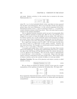
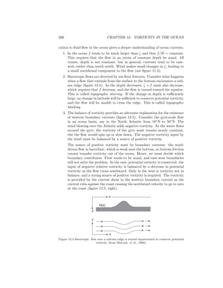
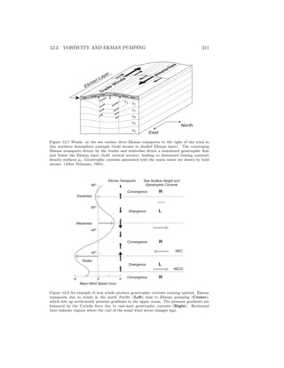
![12.3. VORTICITY AND EKMAN PUMPING 209
Fluid Dynamics on the Beta Plane: Ekman Pumping If (12.16) is true,
the flow cannot expand or contract in the vertical direction, and it is indeed as
rigid as a steel bar. There can be no gradient of vertical velocity in an ocean
with constant planetary vorticity. How then can the divergence of the Ekman
transport at the sea surface lead to vertical velocities at the surface or at the
base of the Ekman layer? The answer can only be that one of the constraints
used in deriving (12.16) must be violated. One constraint that can be relaxed
is the requirement that f = f0.
Consider then flow on a beta plane. If f = f0 + β y, then (12.15a) becomes:
∂u
∂x
+
∂v
∂y
= −
1
f ρ0
∂2
p
∂x ∂y
+
1
f ρ0
∂2
p
∂x ∂y
−
β
f
1
f ρ0
∂p
∂x
(12.17)
f
∂u
∂x
+
∂v
∂y
= −β v (12.18)
where we have used (12.13a) to obtain v in the right-hand side of (12.18).
Using the continuity equation, and recalling that β y f0
f0
∂wG
∂z
= β v (12.19)
where we have used the subscript G to emphasize that (12.19) applies to the
ocean’s interior, geostrophic flow. Thus the variation of Coriolis force with lat-
itude allows vertical velocity gradients in the geostrophic interior of the ocean,
and the vertical velocity leads to north-south currents. This explains why Sver-
drup and Stommel both needed to do their calculations on a β-plane.
Ekman Pumping in the Ocean In Chapter 9, we saw that the curl of the
wind stress T produced a divergence of the Ekman transports leading to a
vertical velocity wE(0) at the top of the Ekman layer. In Chapter 9 we derived
wE(0) = −curl
T
ρf
(12.20)
which is (9.30b) where ρ is density and f is the Coriolis parameter. Because the
vertical velocity at the sea surface must be zero, the Ekman vertical velocity
must be balanced by a vertical geostrophic velocity wG(0).
wE(0) = −wG(0) = −curl
T
ρf
(12.21)
Ekman pumping (wE(0) ) drives a vertical geostrophic current (−wG(0) )
in the ocean’s interior. But why does this produce the northward current cal-
culated by Sverdrup (11.6)? Peter Niiler (1987: 16) gives a simple explanation.
Let us postulate there exists a deep level where horizontal and vertical
motion of the water is much reduced from what it is just below the mixed
layer [figure 12.6]. . . Also let us assume that vorticity is conserved there
(or mixing is small) and the flow is so slow that accelerations over the](https://image.slidesharecdn.com/introductiontophysicaloceanography-130610201256-phpapp02/85/Introduction-to-physical-oceanography-217-320.jpg)
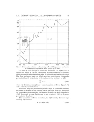
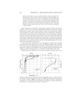
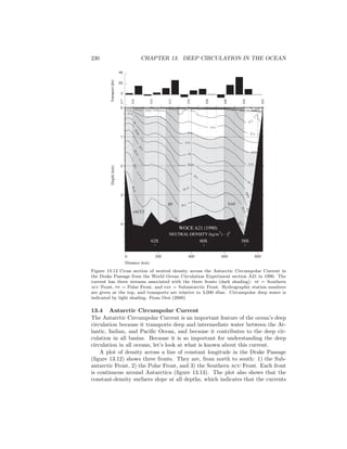
![13.2. THEORY FOR THE THERMOHALINE CIRCULATION 221
S2
S1
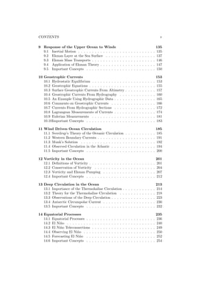
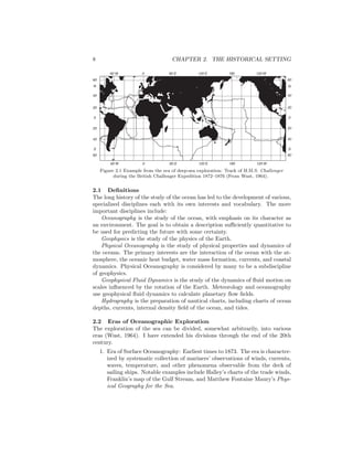
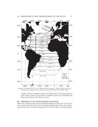
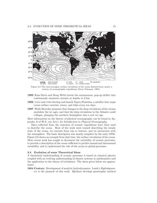
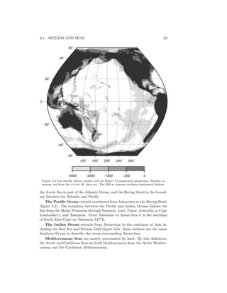
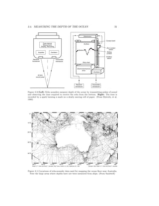
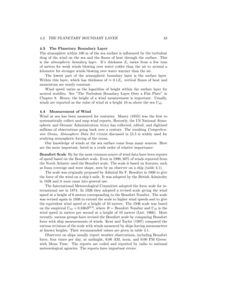
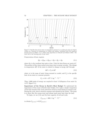
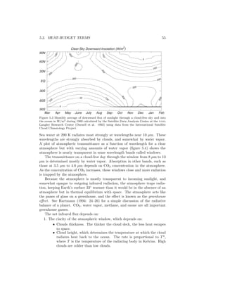
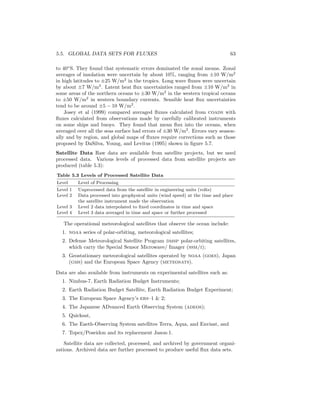
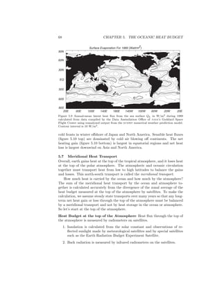
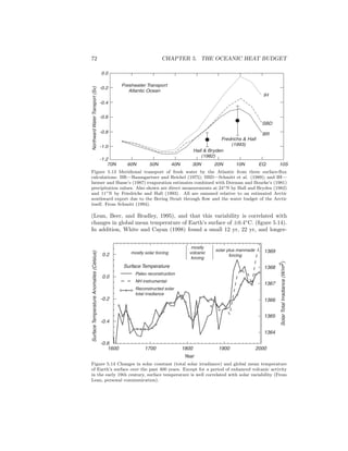
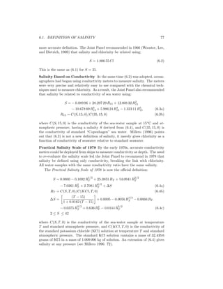
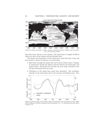
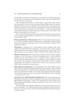
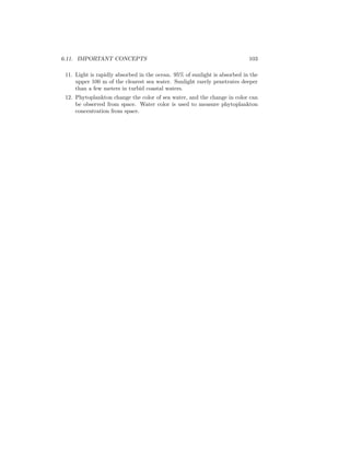
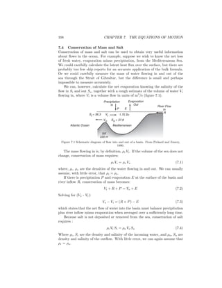
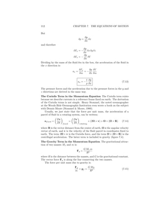
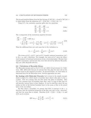
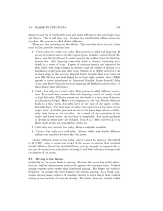
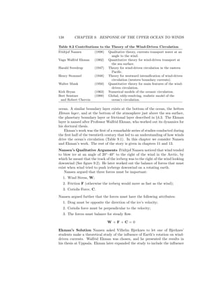
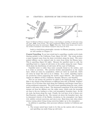
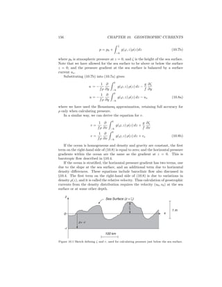
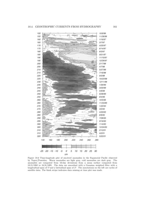
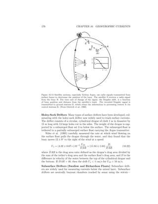
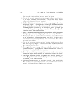
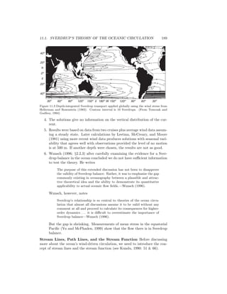
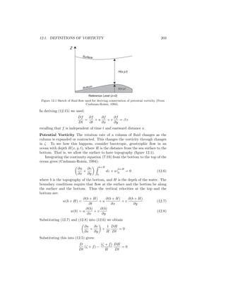
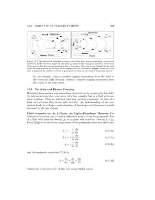
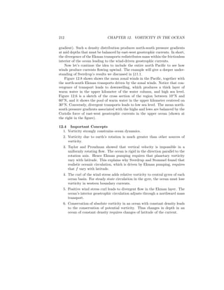
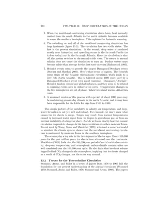
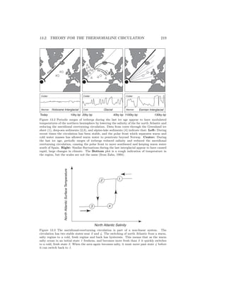
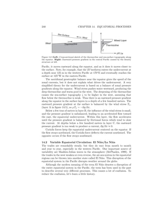
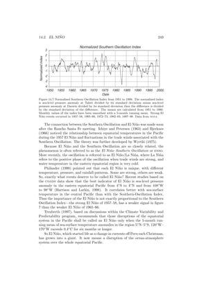
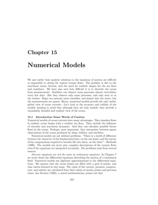
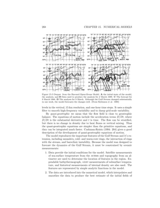
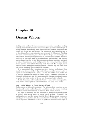
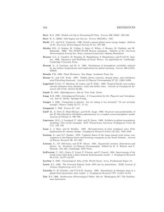
Figure 13.4 Sketch of the deep circulation resulting from deep convection in the Atlantic
(dark circles) and upwelling through the thermocline elsewhere (After Stommel, 1958).
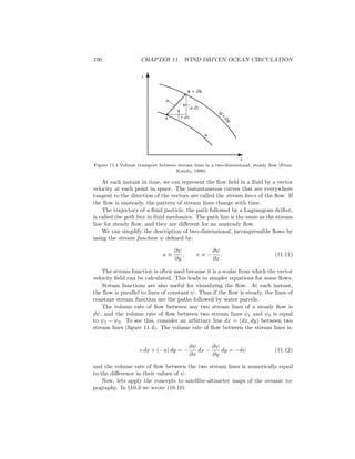
To connect the streamlines of the flow in the west, Stommel added a deep
western boundary current. The strength of the western boundary current de-
pends on the volume of water S produced at the source regions.
Stommel and Arons calculated the flow for a simplified ocean bounded by
the Equator and two meridians (a pie shaped ocean). First they placed the
source S0 near the pole to approximate the flow in the north Atlantic. If the
volume of water sinking at the source equals the volume of water upwelled in the
basin, and if the upwelled velocity is constant everywhere, then the transport
Tw in the western boundary current is:
Tw = −2 S0 sin ϕ (13.3)
The transport in the western boundary current at the poles is twice the volume
of the source, and the transport diminishes to zero at the Equator (Stommel
and Arons, 1960a: eq, 7.3.15; see also Pedlosky, 1996: §7.3). The flow driven by
the upwelling water adds a recirculation equal to the source. If S0 exceeds the
volume of water upwelled in the basin, then the western boundary current carries
water across the Equator. This gives the western boundary current sketched in
the north Atlantic in figure 13.4.
Next, Stommel and Arons calculated the transport in a western boundary
current in a basin with no source. The transport is:
Tw = S [1 − 2 sin ϕ] (13.4)
where S is the transport across the Equator from the other hemisphere. In this
basin Stommel notes:
A current of recirculated water equal to the source strength starts at the
pole and flows toward the source . . . [and] gradually diminishes to zero at
ϕ = 30◦
north latitude. A northward current of equal strength starts at
the equatorial source and also diminishes to zero at 30◦
north latitude.](https://image.slidesharecdn.com/introductiontophysicaloceanography-130610201256-phpapp02/85/Introduction-to-physical-oceanography-229-320.jpg)

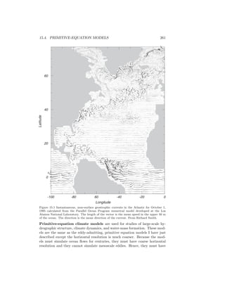
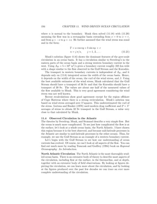
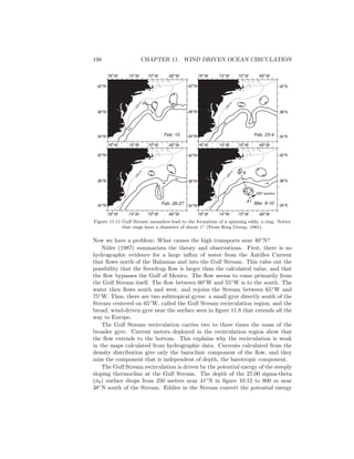
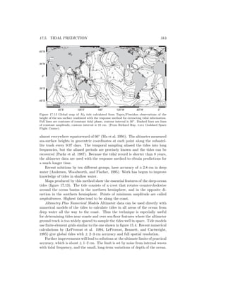
![15.5. COASTAL MODELS 265
. . . both models are able to qualitatively generate many of the observed
features of the flow, but neither is able to quantitatively reproduce de-
tailed currents . . . [Differences] are primarily attributable to inadequate
parameterizations of subgrid scale turbulent mixing, to lack of horizontal
resolution and to imperfect initial and boundary conditions.
Storm-Surge Models Storms coming ashore across wide, shallow, continental
shelves drive large changes of sea level at the coast called storm surges (see
§17.3 for a description of surges and processes influencing surges). The surges
can cause great damage to coasts and coastal structures. Intense storms in the
Bay of Bengal have killed hundreds of thousands in a few days in Bangladesh.
Because surges are so important, government agencies in many countries have
developed models to predict the changes of sea level and the extent of coastal
flooding.
Calculating storm surges is not easy. Here are some reasons, in a rough order
of importance.
1. The distribution of wind over the ocean is not well known. Numerical
weather models calculate wind speed at a constant pressure surface, storm-
surge models need wind at a constant height of 10 m. Winds in bays and
lagoons tend to be weaker than winds just offshore because nearby land
distorts the airflow, and this is not included in the weather models.
2. The shoreward extent of the model’s domain changes with time. For ex-
ample, if sea level rises, water will flood inland, and the boundary between
water and sea moves inland with the water.
3. The drag coefficient of wind on water is not well known for hurricane force
winds.
4. The drag coefficient of water on the seafloor is also not well known.
5. The models must include waves and tides which influence sea level in
shallow waters.
6. Storm surge models must include the currents generated in a stratified,
shallow sea by wind.
To reduce errors, models are tuned to give results that match conditions seen in
past storms. Unfortunately, those past conditions are not well known. Changes
in sea level and wind speed are rarely recorded accurately in storms except at a
few, widely paced locations. Yet storm-surge heights can change by more than
a meter over distances of tens of kilometers.
Despite these problems, models give very useful results. Let’s look at one,
commonly-used model.
Sea, Lake, and Overland Surges Model slosh is used by noaa for forecasting
storm surges produced by hurricanes coming ashore along the Atlantic and Gulf
coasts of the United States (Jelesnianski, Chen, and Shaffer, 1992).
The model is the result of a lifetime of work by Chester Jelesnianski. In
developing the model, Jelesnianski paid careful attention to the relative impor-
tance of errors in the model. He worked to reduce the largest errors, and ignored](https://image.slidesharecdn.com/introductiontophysicaloceanography-130610201256-phpapp02/85/Introduction-to-physical-oceanography-273-320.jpg)
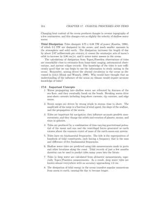
![15.7. COUPLED OCEAN AND ATMOSPHERE MODELS 269
density and velocity. The resulting fields are called an analysis.
3. The model is integrated forward for one week, when new data are available,
to produce a forecast.
4. Finally, the new data are introduced into the model as in the first step
above, and the processes is repeated.
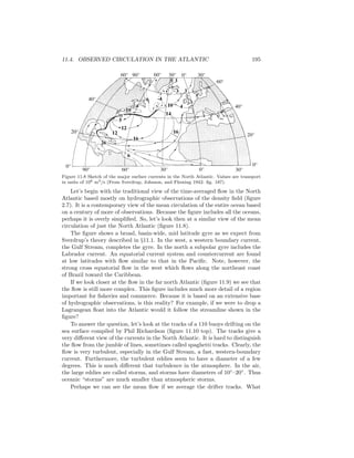
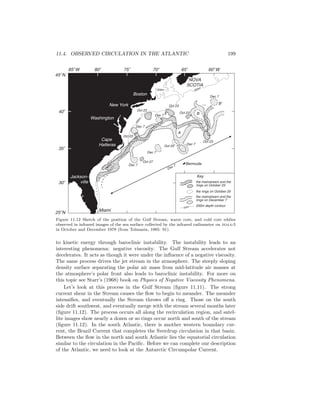
The model has been used for making successful, one-week forecasts of the Gulf
Stream and region (figure 15.4). Similar models have been developed to study
the many other oceanic areas. Starting in 2003, the Global Ocean Data As-
similation Experiment godae will start producing global analyses and forecasts
using models with resolutions of up to 1/16◦
.
15.7 Coupled Ocean and Atmosphere Models
Coupled numerical models of the atmosphere and the ocean are used to study
the climate system, its natural variability, and its response to external forcing.
The most important use of the models has been to study how Earth’s climate
might respond to a doubling of CO2 in the atmosphere. Much of the literature
on climate change is based on studies using such models. Other important uses
of coupled models include studies of El Ni˜no and the meridional overturning
circulation. The former varies over periods of a few years, the latter varies over
a period of a few centuries.
Development of the work tends to be coordinated through the World Climate
Research Program of the World Meteorological Organization wcrp/wmo, and
recent progress is summarized in Chapter 5 of the Climate Change 1995 report
by the Intergovernmental Panel on Climate Change (Gates, et al, 1996).
Comments on Accuracy of Coupled Models Models of the coupled, land-
air-ice-ocean climate system must simulate hundreds to thousands of years. Yet,
It will be very hard to establish an integration framework, particularly
on a global scale, as present capabilities for modelling the Earth system
are rather limited. A dual approach is planned. On the one hand, the
relatively conventional approach of improving coupled atmosphere-ocean-
land-ice models will be pursued. Ingenuity aside, the computational de-
mands are extreme, as is borne out by the Earth System Simulator — 640
linked supercomputers providing 40 teraflops [1012
floating-point opera-
tions per second] and a cooling system from hell under one roof — to be
built in Japan by 2003.— Newton, 1999.
Because models must be simplified to run on existing computers, the models
must be simpler than models that simulate flow for a few years (wcrp, 1995).
In addition, the coupled model must be integrated for many years for the
ocean and atmosphere to approach equilibrium. As the integration proceeds,
the coupled system tends to drift away from reality due to errors in calculating
fluxes of heat and momentum between the ocean and atmosphere. For example,
very small errors in precipitation over the Antarctic Circumpolar Current leads
to small changes the salinity of the current, which leads to large changes in](https://image.slidesharecdn.com/introductiontophysicaloceanography-130610201256-phpapp02/85/Introduction-to-physical-oceanography-277-320.jpg)

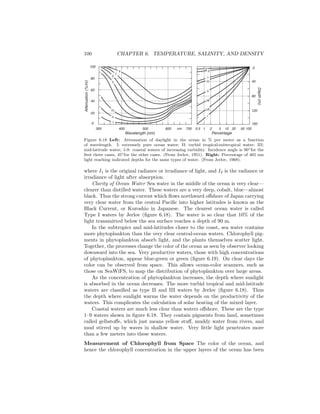
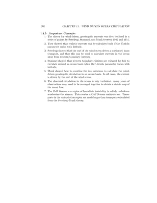
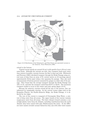
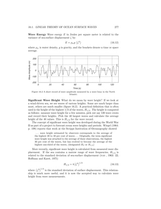
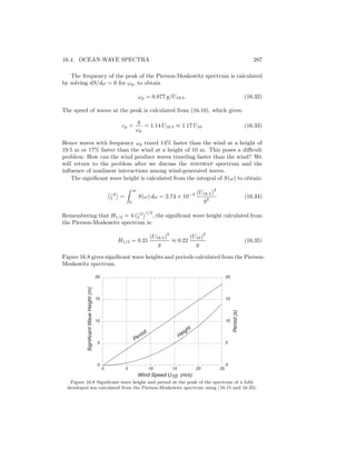
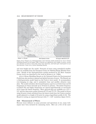
![276 CHAPTER 16. OCEAN WAVES
=121
o
=205
o
9 11 13 15 17 19 21
September 1959
10 10
10
10
.01
.01.01
.01
0.1
1.0
Frequency[mHz]
0.01
0
0.07
0.08
=115
o
=205
o
=126
o
=200
o
=135
o =200
o
0.02
0.03
0.04
0.05
0.06
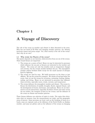
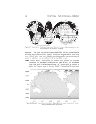
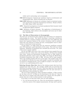
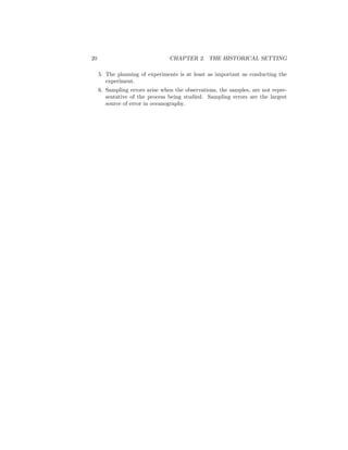
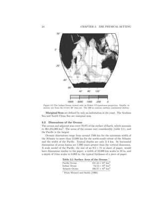
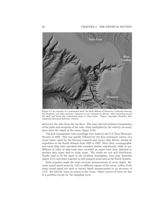
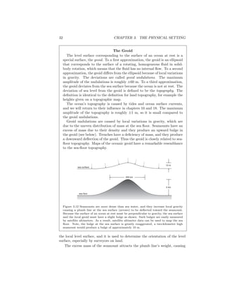
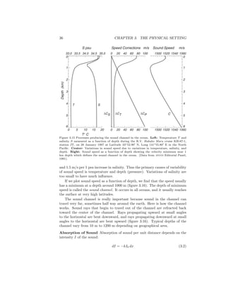
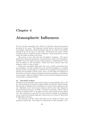
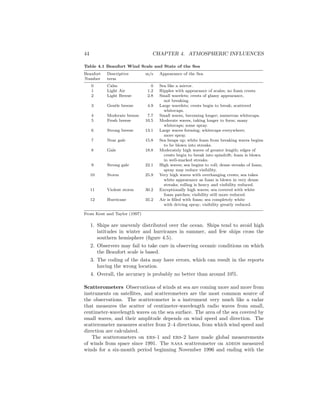
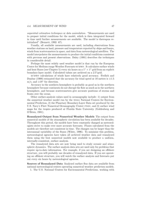
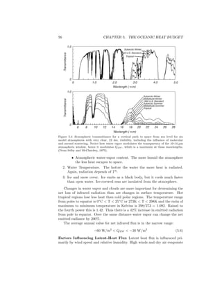
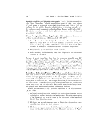
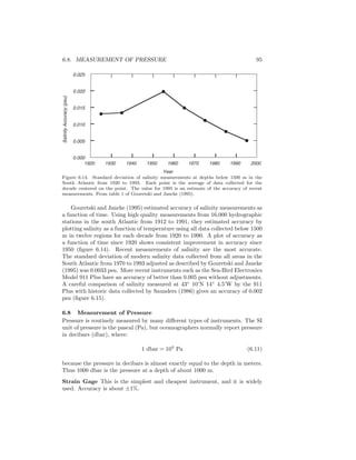
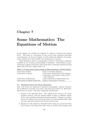
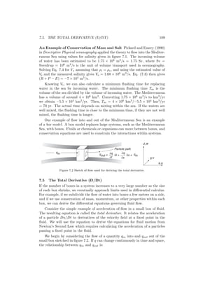
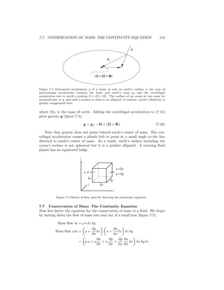
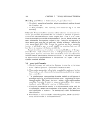
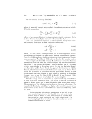
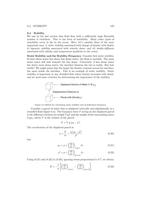
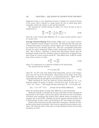
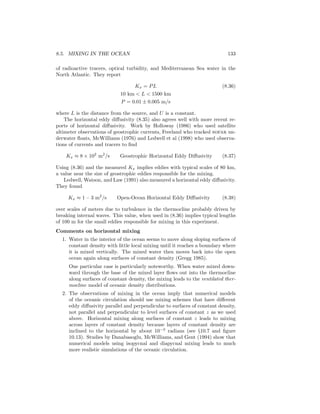
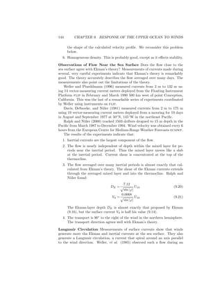
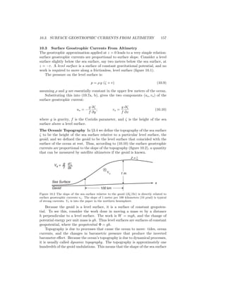
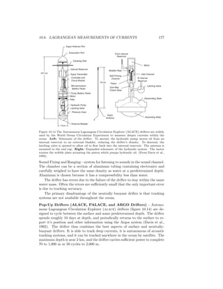
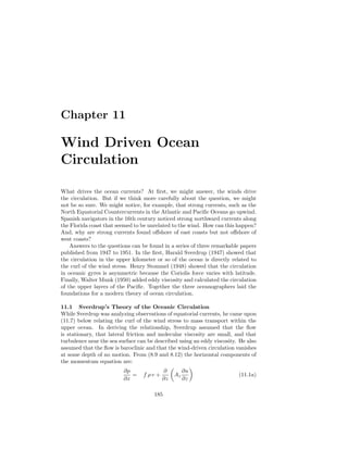
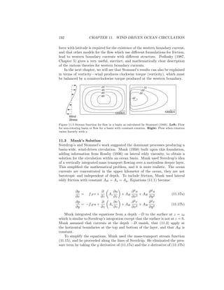
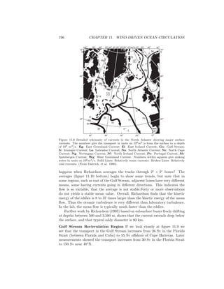
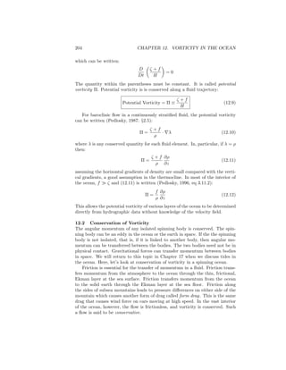
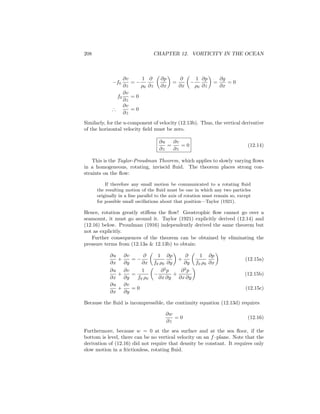
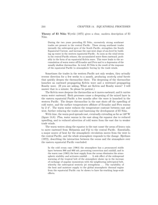
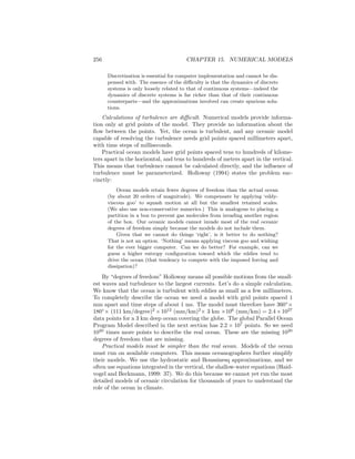
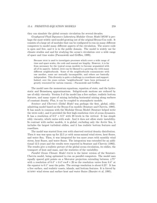
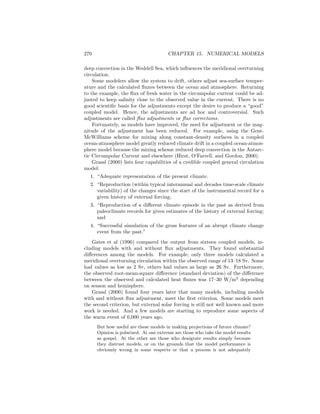
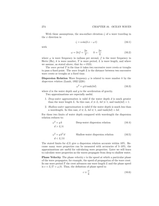
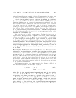
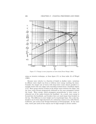
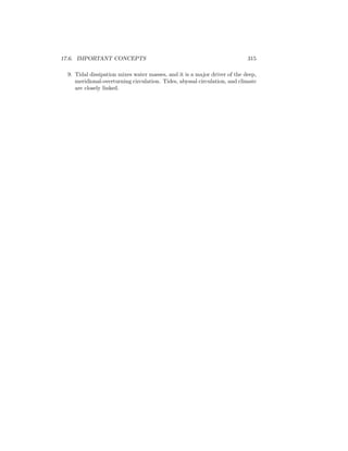
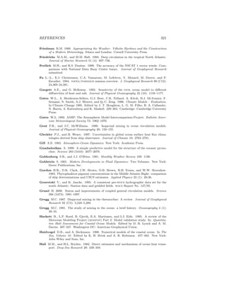
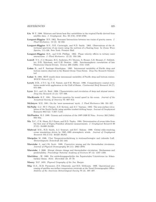
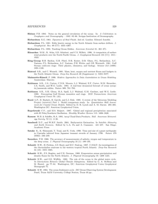
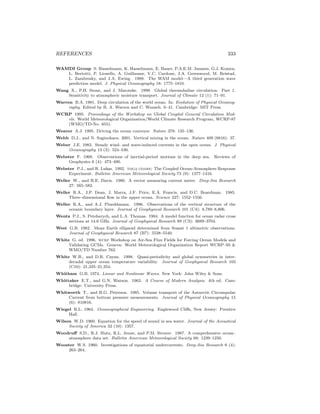
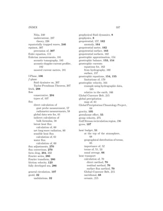
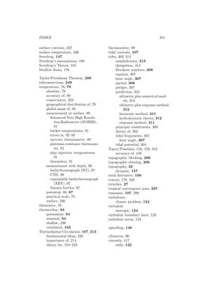
Figure 16.1 Contours of wave energy on a frequency-time plot calculated from spectra of
waves measured by pressure gauges offshore of southern California. The ridges of high wave
energy show the arrival of dispersed wave trains from distant storms. The slope of the ridge
is inversely proportional to distance to the storm. ∆ is distance in degrees, θ is direction of
arrival of waves at California (from Munk et al. 1963).
calculated for each day’s data. (The concept of a spectra is discussed below.)
From the spectra, the amplitudes and frequencies of the low-frequency waves
and the propagation direction of the waves were calculated. Finally, they plotted
contours of wave energy on a frequency-time diagram (figure 16.1).
To understand the figure, consider a distant storm that produces waves of
many frequencies. The lowest-frequency waves (smallest ω) travel the fastest
(16.11), and they arrive before other, higher-frequency waves. The further away
the storm, the longer the delay between arrivals of waves of different frequencies.
The ridges of high wave energy seen in the figure are produced by individual
storms. The slope of the ridge gives the distance to the storm in degrees ∆
along a great circle; and the phase information from the array gives the angle to
the storm θ. The two angles give the storm’s location relative to San Clemente.
Thus waves arriving from 15 to 18 September produce a ridge indicating the
storm was 115◦
away at an angle of 205◦
which is south of new Zealand near
Antarctica.
The locations of the storms producing the waves recorded from June through
October 1959 were compared with the location of storms plotted on weather
maps and in most cases the two agreed well.](https://image.slidesharecdn.com/introductiontophysicaloceanography-130610201256-phpapp02/85/Introduction-to-physical-oceanography-284-320.jpg)
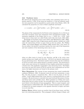
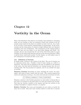
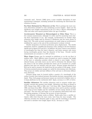
![282 CHAPTER 16. OCEAN WAVES
Time, j∆ [s]
0 5 10 15 20
-200
-100
0
100
200
WaveHeight,ζj[m]
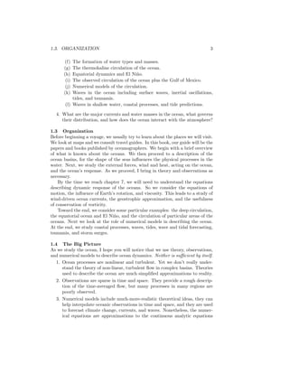
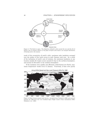
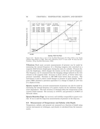
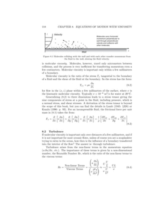
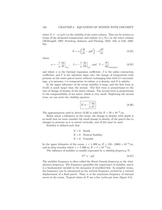
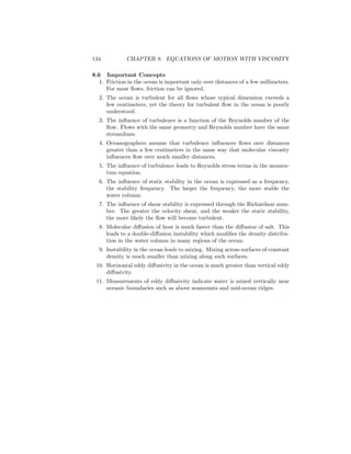
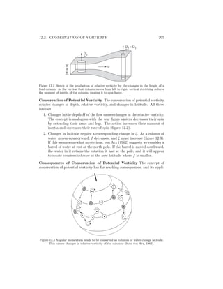
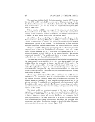
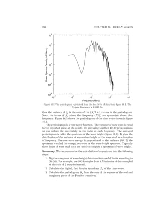
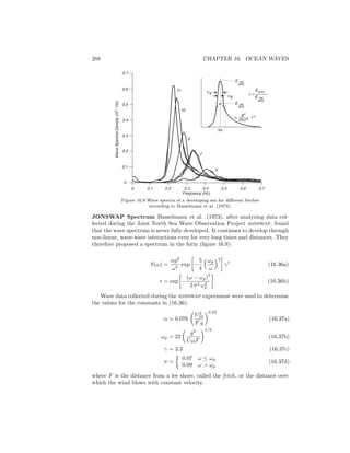
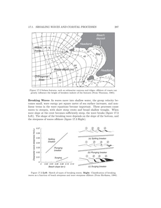
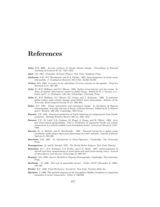
Figure 16.3 The first 20 seconds of digitized data from figure 16.2. ∆ = 0.32 s.
The sampling interval ∆ defines a Nyquist critical frequency (Press et al,
1992: 494)
Ny ≡ 1/(2∆) (16.25)
The Nyquist critical frequency is important for two related, but dis-
tinct, reasons. One is good news, the other is bad news. First the good
news. It is the remarkable fact known as the sampling theorem: If a con-
tinuous function ζ(t), sampled at an interval ∆, happens to be bandwidth
limited to frequencies smaller in magnitude than Ny, i.e., if S(nf) = 0
for all |nf| ≥ Ny, then the function ζ(t) is completely determined by its
samples ζj . . . This is a remarkable theorem for many reasons, among
them that it shows that the “information content” of a bandwidth lim-
ited function is, in some sense, infinitely smaller than that of a general
continuous function . . .
Now the bad news. The bad news concerns the effect of sampling a
continuous function that is not bandwidth limited to less than the Nyquist
critical frequency. In that case, it turns out that all of the power spectral
density that lies outside the frequency range −Ny ≤ nf ≤ Ny is spuri-
ously moved into that range. This phenomenon is called aliasing. Any
frequency component outside of the range (−Ny, Ny) is aliased (falsely
translated) into that range by the very act of discrete sampling . . . There
is little that you can do to remove aliased power once you have discretely
sampled a signal. The way to overcome aliasing is to (i) know the natural
bandwidth limit of the signal — or else enforce a known limit by analog
filtering of the continuous signal, and then (ii) sample at a rate sufficiently
rapid to give at least two points per cycle of the highest frequency present.
—Press et al 1992, but with notation changed to our notation.
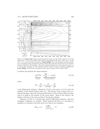
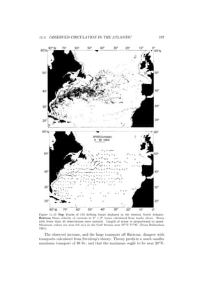
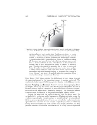
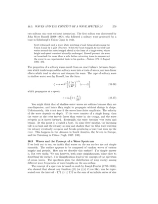
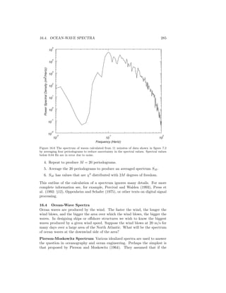
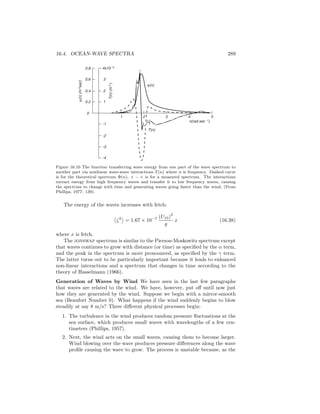
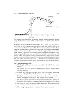
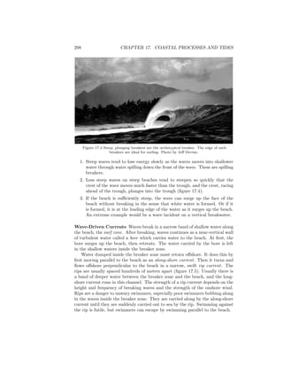
Figure 16.4 illustrates the aliasing problem. Notice how a high frequency
signal is aliased into a lower frequency if the higher frequency is above the
critical frequency. Fortunately, we can can easily avoid the problem: (i) use
instruments that do not respond to very short, high frequency waves if we are
interested in the bigger waves; and (ii) chose ∆t small enough that we lose little
useful information. In the example shown in figure 16.3, there are no waves in
the signal to be digitized with frequencies higher than Ny = 1.5625 Hz.
Let’s summarize. Digitized signals from a wave staff cannot be used to study
waves with frequencies above the Nyquist critical frequency. Nor can the signal](https://image.slidesharecdn.com/introductiontophysicaloceanography-130610201256-phpapp02/85/Introduction-to-physical-oceanography-290-320.jpg)
![16.3. WAVES AND THE CONCEPT OF A WAVE SPECTRUM 283
t = 0.2 s
f = 4 Hz f = 1 Hz
one second
Figure 16.4 Sampling a 4 Hz sine wave (heavy line) every 0.2 s aliases the frequency to 1 Hz
(light line). The critical frequency is 1/(2 × 0.2 s) = 2.5 Hz, which is less than 4 Hz.
be used to study waves with frequencies less than the fundamental frequency
determined by the duration T of the wave record. The digitized wave record
contains information about waves in the frequency range:
1
T
< f <
1
2∆
(16.26)
where T = N∆ is the length of the time series, and f is the frequency in Hertz.
Calculating The Wave Spectrum The digital Fourier transform Zn of a
wave record ζj equivalent to (16.21 and 16.22) is:
Zn =
1
N
N−1
j=0
ζj exp[−i2πjn/N] (16.27a)
ζn =
N−1
n=0
Zj exp[i2πjn/N] (16.27b)
for j = 0, 1, · · · , N − 1; n = 0, 1, · · · , N − 1. These equations can be summed
very quickly using the Fast Fourier Transform, especially if N is a power of 2
(Cooley, Lewis, and Welch, 1970; Press et al. 1992: 542).
The simple spectrum Sn of ζ, which is called the periodogram, is:
Sn =
1
N2
|Zn|2
+ |ZN−n|2
; n = 1, 2, · · · , (N/2 − 1) (16.28)
S0 =
1
N2
|Z0|2
SN/2 =
1
N2
|ZN/2|2
where SN is normalized such that:
N−1
j=0
|ζj|2
=
N/2
n=0
Sn (16.29)](https://image.slidesharecdn.com/introductiontophysicaloceanography-130610201256-phpapp02/85/Introduction-to-physical-oceanography-291-320.jpg)
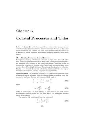
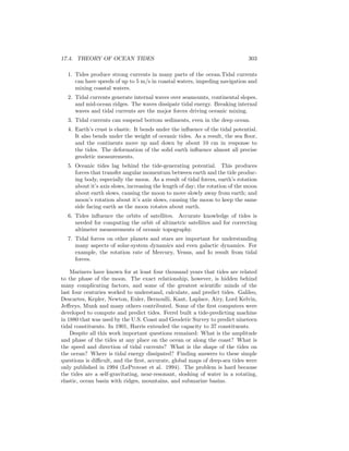
![306 CHAPTER 17. COASTAL PROCESSES AND TIDES
observer on earth, the two tidal bulges seems to rotate around earth because
moon appears to move around the sky at nearly one cycle per day. Moon
produces high tides every 12 hours and 25.23 minutes on the equator if the
moon is above the equator. Notice that high tides are not exactly twice per day
because the moon is also rotating around earth. Of course, the moon is above
the equator only twice per lunar month, and this complicates our simple picture
of the tides on an ideal ocean-covered earth. Furthermore, moon’s distance from
earth R varies because moon’s orbit is elliptical and because the elliptical orbit
is not fixed.
Clearly, the calculation of tides is getting more complicated than we might
have thought. Before continuing on, we note that the solar tidal forces are
derived in a similar way. The relative importance of the sun and moon are
nearly the same. Although the sun is much more massive than moon, it is much
further away.
Gsun = GS =
3
4
γS
r2
R3
sun
(17.12)
Gmoon = GM =
3
4
γM
r2
R3
moon
(17.13)
GS
GM
= 0.46051 (17.14)
where Rsun is the distance to the sun, S is the mass of the sun, Rmoon is the
distance to the moon, and M is the mass of the moon.
Coordinates of Sun and Moon Before we can proceed further we need to
know the position of moon and sun relative to earth. An accurate description of
the positions in three dimensions is very difficult, and it involves learning arcane
terms and concepts from celestial mechanics. Here, I paraphrase a simplified
description from Pugh. See also figure 4.1.
A natural reference system for an observer on earth is the equatorial system
described at the start of Chapter 3. In this system, declinations δ of a celestial
body are measured north and south of a plane which cuts the earth’s equator.
Angular distances around the plane are measured relative to a point
on this celestial equator which is fixed with respect to the stars. The
point chosen for this system is the vernal equinox, also called the ‘First
Point of Aries’ . . . The angle measured eastward, between Aries and the
equatorial intersection of the meridian through a celestial object is called
the right ascension of the object. The declination and the right ascension
together define the position of the object on a celestial background . . .
[Another natural reference] system uses the plane of the earth’s revo-
lution around the sun as a reference. The celestial extension of this plane,
which is traced by the sun’s annual apparent movement, is called the
ecliptic. Conveniently, the point on this plane which is chosen for a zero
reference is also the vernal equinox, at which the sun crosses the equato-
rial plane from south to north near 21 March each year. Celestial objects
are located by their ecliptic latitude and ecliptic longitude. The angle](https://image.slidesharecdn.com/introductiontophysicaloceanography-130610201256-phpapp02/85/Introduction-to-physical-oceanography-314-320.jpg)
![17.4. THEORY OF OCEAN TIDES 309
If the ellipticity of the orbit is small, R = R0(1+ ), and (17.18) is approximately
V = a(1 − 3 ) cos (4πf1) (17.19)
where a = γMr2
/ 4R3
is a constant. varies with a period of 27.32 days,
and we can write = b cos(2πf2) where b is a small constant. With these
simplifications, (17.19) can be written:
V = a cos (4πf1) − 3ab cos (2πf2) cos (4πf1) (17.20a)
V = a cos (4πf1) − 3ab [cos 2π (2f1 − f2) + cos 2π (2f1 + f2)] (17.20b)
which has a spectrum with three lines at 2f1 and 2f1 ± f2. Therefore, the slow
modulation of the amplitude of the tidal potential at two cycles per lunar day
causes the potential to be split into three frequencies. This is the way amplitude
modulated AM radio works. If we add in the the slow changes in the shape of
the orbit, we get still more terms even in this very idealized case of a moon in
an equatorial orbit.
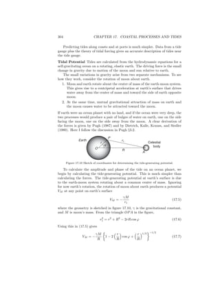
If you are very observant, you will have noticed that the spectrum of the
tide waves in figure 17.12 does not look like the spectrum of ocean waves in
figure 16.6. Ocean waves have all possible frequencies, and their spectrum is
continuous. Tides have precise frequencies determined by the orbit of earth and
moon, and their spectrum is not continuous. It consists of discrete lines.
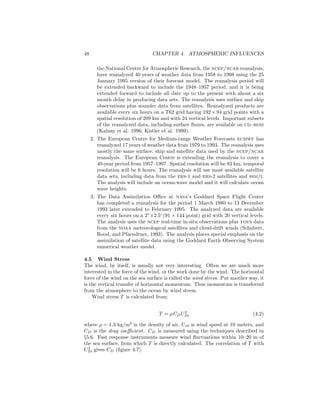
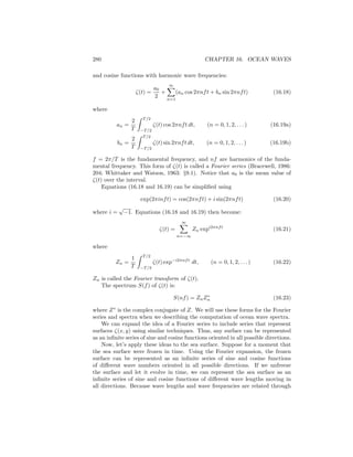
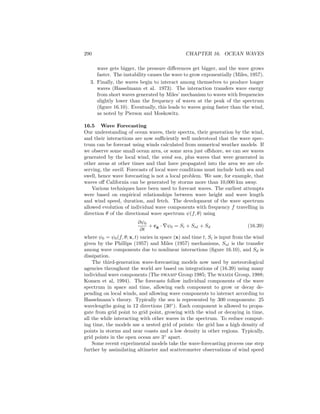
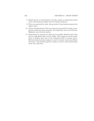
Doodson’s expansion included 399 constituents, of which 100 are long period,
160 are daily, 115 are twice per day, and 14 are thrice per day. Most have very
small amplitudes, and only the largest are included in table 17.2. The largest
Table 17.2 Principal Tidal Constituents
Equilibrium
Tidal Amplitude† Period
Species Name n1 n2 n3 n4 n5 (m) (hr)
Semidiurnal n1 = 2
Principal lunar M2 2 0 0 0 0 0.242334 12.4206
Principal solar S2 2 2 -2 0 0 0.112841 12.0000
Lunar elliptic N2 2 -1 0 1 0 0.046398 12.6584
Lunisolar K2 2 2 0 0 0 0.030704 11.9673
Diurnal n1 = 1
Lunisolar K1 1 1 0 0 0 0.141565 23.9344
Principal lunar O1 1 -1 0 0 0 0.100514 25.8194
Principal solar P1 1 1 -2 0 0 0.046843 24.0659
Elliptic lunar Q1 1 -2 0 1 0 0.019256 26.8684
Long Period n1 = 0
Fortnightly Mf 0 2 0 0 0 0.041742 327.85
Monthly Mm 0 1 0 -1 0 0.022026 661.31
Semiannual Ssa 0 0 2 0 0 0.019446 4383.05
†Amplitudes from Apel (1987)](https://image.slidesharecdn.com/introductiontophysicaloceanography-130610201256-phpapp02/85/Introduction-to-physical-oceanography-317-320.jpg)


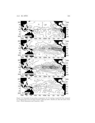
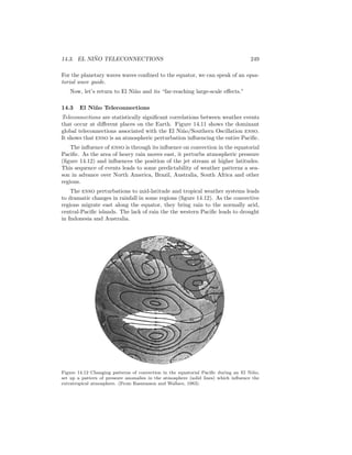
This document is an introduction to physical oceanography textbook written by Robert H. Stewart. It is divided into 17 chapters that cover topics such as the historical context of oceanographic exploration, the physical properties and dynamics of the ocean, atmospheric influences on the ocean, ocean circulation patterns, ocean waves, tides, and coastal processes. The textbook is intended to provide students with the foundational concepts and theoretical framework of physical oceanography.


