Download to read offline

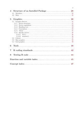
![Chapter 1: R Internal Structures 7
direct access is normally only used to check if the attributes are NULL or to reset them. Otherwise
access goes through the functions getAttrib and setAttrib which impose restrictions on the
attributes. One thing to watch is that if you copy attributes from one object to another you
may (un)set the "class" attribute and so need to copy the object and S4 bits as well. There is
a macro/function DUPLICATE_ATTRIB to automate this.
Note that the ‘attributes’ of a CHARSXP are used as part of the management of the CHARSXP
cache: of course CHARSXP’s are not user-visible but C-level code might look at their attributes.
The code assumes that the attributes of a node are either R_NilValue or a pairlist of non-
zero length (and this is checked by SET_ATTRIB). The attributes are named (via tags on the
pairlist). The replacement function attributes<- ensures that "dim" precedes "dimnames" in
the pairlist. Attribute "dim" is one of several that is treated specially: the values are checked,
and any "names" and "dimnames" attributes are removed. Similarly, you cannot set "dimnames"
without having set "dim", and the value assigned must be a list of the correct length and with
elements of the correct lengths (and all zero-length elements are replaced by NULL).
The other attributes which are given special treatment are "names", "class", "tsp",
"comment" and "row.names". For pairlist-like objects the names are not stored as an attribute
but (as symbols) as the tags: however the R interface makes them look like conventional at-
tributes, and for one-dimensional arrays they are stored as the first element of the "dimnames"
attribute. The C code ensures that the "tsp" attribute is an REALSXP, the frequency is positive
and the implied length agrees with the number of rows of the object being assigned to. Classes
and comments are restricted to character vectors, and assigning a zero-length comment or class
removes the attribute. Setting or removing a "class" attribute sets the object bit appropriately.
Integer row names are converted to and from the internal compact representation.
Care needs to be taken when adding attributes to objects of the types with non-standard
copying semantics. There is only one object of type NILSXP, R_NilValue, and that should
never have attributes (and this is enforced in installAttrib). For environments, external
pointers and weak references, the attributes should be relevant to all uses of the object: it is for
example reasonable to have a name for an environment, and also a "path" attribute for those
environments populated from R code in a package.
When should attributes be preserved under operations on an object? Becker, Chambers &
Wilks (1988, pp. 144–6) give some guidance. Scalar functions (those which operate element-
by-element on a vector and whose output is similar to the input) should preserve attributes
(except perhaps class, and if they do preserve class they need to preserve the OBJECT and S4
bits). Binary operations normally call copyMostAttributes to copy most attributes from the
longer argument (and if they are of the same length from both, preferring the values on the
first). Here ‘most’ means all except the names, dim and dimnames which are set appropriately
by the code for the operator.
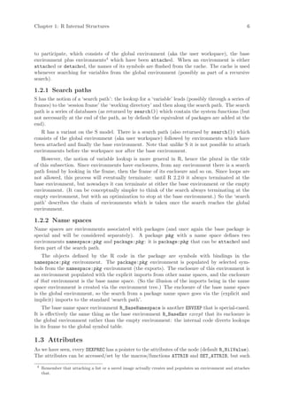
Subsetting (other than by an empty index) generally drops all attributes except names, dim
and dimnames which are reset as appropriate. On the other hand, subassignment generally
preserves such attributes even if the length is changed. Coercion drops all attributes. For
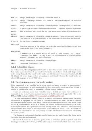
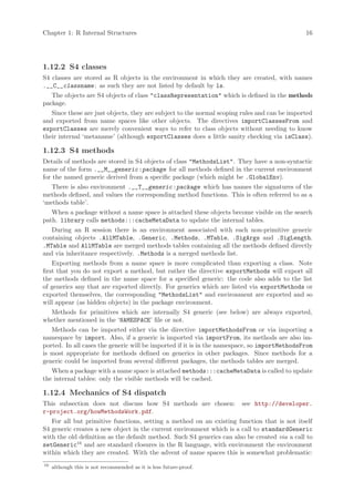
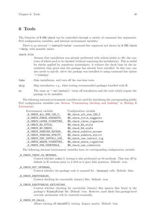
example:
> x <- structure(1:8, names=letters[1:8], comm="a comment")
> x[]
a b c d e f g h
1 2 3 4 5 6 7 8
attr(,"comm")
[1] "a comment"
> x[1:3]
a b c
1 2 3](https://image.slidesharecdn.com/r-ints-091214115349-phpapp01/85/R-Ints-11-320.jpg)
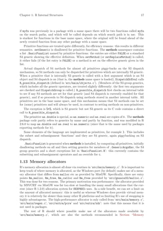
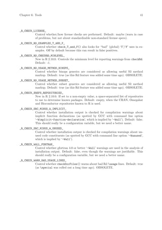
![Chapter 1: R Internal Structures 8
> x[3] <- 3
> x
a b c d e f g h
1 2 3 4 5 6 7 8
attr(,"comm")
[1] "a comment"
> x[9] <- 9
> x
a b c d e f g h
1 2 3 4 5 6 7 8 9
attr(,"comm")
[1] "a comment"
1.4 Contexts
Contexts are the internal mechanism used to keep track of where a computation has got to
(and from where), so that control-flow constructs can work and reasonable information can be
produced on error conditions, (such as via traceback) and otherwise (the sys.xxx functions).
Execution contexts are a stack of C structs:
typedef struct RCNTXT {
struct RCNTXT *nextcontext; /* The next context up the chain */
int callflag; /* The context ‘type’ */
JMP_BUF cjmpbuf; /* C stack and register information */
int cstacktop; /* Top of the pointer protection stack */
int evaldepth; /* Evaluation depth at inception */
SEXP promargs; /* Promises supplied to closure */
SEXP callfun; /* The closure called */
SEXP sysparent; /* Environment the closure was called from */
SEXP call; /* The call that effected this context */
SEXP cloenv; /* The environment */
SEXP conexit; /* Interpreted on.exit code */
void (*cend)(void *); /* C on.exit thunk */
void *cenddata; /* Data for C on.exit thunk */
char *vmax; /* Top of the R_alloc stack */
int intsusp; /* Interrupts are suspended */
SEXP handlerstack; /* Condition handler stack */
SEXP restartstack; /* Stack of available restarts */
struct RPRSTACK *prstack; /* Stack of pending promises */
} RCNTXT, *context;
plus additional fields for the future byte-code compiler. The ‘types’ are from
enum {
CTXT_TOPLEVEL = 0, /* toplevel context */
CTXT_NEXT = 1, /* target for next */
CTXT_BREAK = 2, /* target for break */
CTXT_LOOP = 3, /* break or next target */
CTXT_FUNCTION = 4, /* function closure */
CTXT_CCODE = 8, /* other functions that need error cleanup */
CTXT_RETURN = 12, /* return() from a closure */
CTXT_BROWSER = 16, /* return target on exit from browser */
CTXT_GENERIC = 20, /* rather, running an S3 method */
CTXT_RESTART = 32, /* a call to restart was made from a closure */](https://image.slidesharecdn.com/r-ints-091214115349-phpapp01/85/R-Ints-12-320.jpg)
![Chapter 1: R Internal Structures 15
1.11 Warnings and errors
Each of warning and stop have two C-level equivalents, warning, warningcall, error and
errorcall. The relationship between the pairs is similar: warning tries to fathom out a suitable
call, and then calls warningcall with that call as the first argument if it succeeds, and with
call = R_NilValue it is does not. When warningcall is called, it includes the deparsed call in
its printout unless call = R_NilValue.
warning and error look at the context stack. If the topmost context is not of type CTXT_
BUILTIN, it is used to provide the call, otherwise the next context provides the call. This means
that when these function are called from a primitive or .Internal, the imputed call will not be
to primitive/.Internal but to the function calling the primitive/.Internal . This is exactly
what one wants for a .Internal, as this will give the call to the closure wrapper. (Further,
for a .Internal, the call is the argument to .Internal, and so may not correspond to any R
function.) However, it is unlikely to be what is needed for a primitive.
The upshot is that that warningcall and errorcall should normally be used for code called
from a primitive, and warning and error should be used for code called from a .Internal (and
necessarily from .Call, .C and so on, where the call is not passed down). However, there are
two complications. One is that code might be called from either a primitive or a .Internal,
in which case probably warningcall is more appropriate. The other involves replacement
functions, where the call will be of the form (from R < 2.6.0)
> length(x) <- y ~ x
Error in "length<-"(‘*tmp*‘, value = y ~ x) : invalid value
which is unpalatable to the end user. For replacement functions there will be a suitable context
at the top of the stack, so warning should be used. (The results for .Internal replacement
functions such as substr<- are not ideal.)
1.12 S4 objects
[This section is currently a preliminary draft and should not be taken as definitive. The descrip-
tion assumes that R_NO_METHODS_TABLES has not been set.]
1.12.1 Representation of S4 objects
[The internal representation of objects from S4 classes changed in R 2.4.0. It is possible that
objects from earlier representations still exist, but there is no guarantee that they will be handled
correctly. An attempt is made to detect old-style S4 objects and warn when binary objects are
loaded or a workspace is restored.]
S4 objects can be of any SEXPTYPE. They are either an object of a simple type (such as
an atomic vector or function) with S4 class information or of type S4SXP. In all cases, the
‘S4 bit’ (bit 4 of the ‘general purpose’ field) is set, and can be tested by the macro/function
IS_S4_OBJECT.
S4 objects are created via new()15 and thence via the C function R_do_new_object. This
duplicates the prototype of the class, adds a class attribute and sets the S4 bit. All S4 class
attributes should be character vectors of length one with an attribute giving (as a character
string) the name of the package (or .GlobalEnv) containing the class definition. Since S4
objects have a class attribute, the OBJECT bit is set.
It is currently unclear what should happen if the class attribute is removed from an S4 object,
or if this should be allowed.
15
This can also create non-S4 objects, as in new("integer").](https://image.slidesharecdn.com/r-ints-091214115349-phpapp01/85/R-Ints-19-320.jpg)

![Chapter 1: R Internal Structures 20
X11 (Unix-alikes only.) The X11(), jpeg(), png() and tiff() devices. These are
optional, and links to some or all of the X11, pango, cairo, jpeg, libpng and
libtiff libraries.
‘Rbitmap.dll’
(Windows only.) The code for the BMP, JPEG, PNG and TIFF devices and for
saving on-screen graphs to those formats. This is technically optional, and needs
source code not in the tarball.
‘internet2.dll’
(Windows only.) An alternative version of the internet access routines, compiled
against Internet Explorer internals (and so loads ‘wininet.dll’ and ‘wsock32.dll’).
1.16 Visibility
1.16.1 Hiding C entry points
We make use of the visibility mechanisms discussed in Section “Controlling visibility” in Writing
R Extensions, C entry points not needed outside the main R executable/dynamic library (and
in particular in no package nor module) should be prefixed by attribute_hidden. Minimizing
the visibility of symbols in the R dynamic library will speed up linking to it (which packages
will do) and reduce the possibility of linking to the wrong entry points of the same name. In
addition, on some platforms reducing the number of entry points allows more efficient versions
of PIC to be used: somewhat over half the entry points are hidden. A convenient way to hide
variables (as distinct from functions) is to declare them extern0 in ‘Defn.h’.
The visibility mechanism used is only available with some compilers and platforms, and in
particular not on Windows, where are alternative mechanism is used. Entry points will not be
made available in ‘R.dll’ if they are listed in the file ‘src/gnuwin32/Rdll.hide’. Entries in
that file start with a space and must be strictly in alphabetic order in the C locale (use sort on
the file to ensure this if you change it). It is possible to hide Fortran as well as C entry points via
this file: the former are lower-cased and have an underline as suffix, and the suffixed name should
be included in the file. Some entry points exist only on Windows or need to be visible only on
Windows, and some notes on these are provided in file ‘src/gnuwin32/Maintainters.notes’.
Because of the advantages of reducing the number of visible entry points, they should be
declared attribute_hidden where possible. Note that this only has an effect on a shared-
R-library build, and so care is needed not to hide entry points that are legitimately used by
packages. So it is best if the decision on visibility is made when a new entry point is created,
including the decision if it should be included in ‘Rinternals.h’. A list of the visible entry points
on shared-R-library build on a reasonably standard Unix-alike can be made by something like
nm -g libR.so | grep ’ [BCDT] ’ | cut -b20-
1.16.2 Variables in Windows DLLs
Windows is unique in that it conventionally treats importing variables differently from functions:
variables that are imported from a DLL need to be specified by a prefix (often ‘_imp_’) when
being linked to (‘imported’) but not when being linked from (‘exported’). The details depend
on the compiler system, and have changed for MinGW during the lifetime of that port. They
are in the main hidden behind some macros defined in header ‘R_ext/libextern.h’.
A (non-function) variable in the main R sources that needs to be referred to outside ‘R.dll’
(in a package, module or another DLL such as ‘Rgraphapp.dll’) should be declared with prefix
LibExtern. The main use is in ‘Rinternals.h’, but it needs to be considered for any public
header and also ‘Defn.h’.
It would nowadays be possible to make use of the ‘auto-import’ feature of the MinGW port of
ld to fix up imports from DLLs (and if R is built for the Cygwin platform this is what happens).](https://image.slidesharecdn.com/r-ints-091214115349-phpapp01/85/R-Ints-24-320.jpg)
![Chapter 4: Structure of an Installed Package 28
4 Structure of an Installed Package
The structure of a source packages is described in Section “Creating R packages” in Writing R
Extensions: this chapter is concerned with the structure of installed packages.
The description here is for R 2.10.0 and later: the way help was installed differed in earlier
versions.
An installed package has a top-level file ‘DESCRIPTION’, a copy of the file of that name
in the package sources with a ‘Built’ field appended, and file ‘INDEX’, usually describing the
objects on which help is available, a file ‘NAMESPACE’ is the package has a name space, files such
as ‘CITATION’, ‘LICENCE’ and ‘NEWS’, and any other files copied in from ‘inst’. It will have
directories ‘Meta’, ‘help’ and ‘html’ (even if the package has no help), almost always has a
directory ‘R’ and often has a directory ‘libs’ to contain compiled code. Other directories with
known meaning to R are ‘data’, ‘demo’, ‘doc’ and ‘po’.
Function library looks for a name space and if one is found passes control to loadNamespace.
Then library or loadNamespace looks for file ‘R/pkgname ’, warns if it is not found and otherwise
sources the code (using sys.source) into the package’s environment, then lazy-load a database
‘R/sysdata’ if present. So how R code gets loaded depends on the contents of ‘R/pkgname ’:
standard templates to load lazy-load databases are provided in ‘share/R/[ns]packloader.R’.
How (and if) compiled code is loaded is down to the package’s start-code such as .First.lib
or .onLoad, although a useDynlib directive in a name space provides an alternative. Conven-
tionally compiled code is loaded by a call to library.dynam and this looks in directory ‘libs’
(and in an appropriate sub-directory if sub-architectures are in use) for a shared object (Unix-
alike) or DLL (Windows).
Subdirectory ‘data’ serves two purposes. In a package using lazy-loading of data, it contains
a lazy-load database ‘Rdata’, plus a file ‘Rdata.rds’ which contain a named character vector
used by data in the (unusual) event that it is used for such a package. Otherwise it is copy of the
‘data’ directory in the sources, with saved images re-compressed if R CMD INSTALL --resave-
data was used. If R CMD INSTALL --use-data-zip was specified or selected via ‘--auto-zip’,
the contents of the directory are moved to a zip file ‘Rdata.zip’ and a listing written in file
‘filelist’.
Subdirectory ‘demo’ supports the demo function, and is copied from the sources.
Subdirectory ‘po’ contains (in subdirectories) compiled message catalogs.
4.1 Metadata
Directory ‘Meta’ contains several files in .rds format, that is saved R objects. All packages have
‘Rd.rds’, ‘hsearch.rds’, ‘links.rds’ and ‘package.rds’. Packages with name spaces have
a file ‘nsInfo.rds’, and those with data, demos or vignettes have ‘data.rds’, ‘demo.rds’ or
‘vignette.rds’ files.
The structure of these files (and their existence and names) is private to R, so the description
here is for those trying to follow the R sources: there should be no reference to these files in
non-base packages.
File ‘package.rds’ is a dump of information extracted from the ‘DESCRIPTION’ file. It is a
list of several components. The first, ‘DESCRIPTION’, is a character vector, the ‘DESCRIPTION’
file as read by read.dcf. Further elements ‘Depends’, ‘Suggests’, ‘Imports’, ‘Rdepends’ and
‘Rdepends2’ record the ‘Depends’, ‘Suggests’ and ‘Imports’ fields. These are all lists, and can
be empty. The first three have an entry for each package named, each entry being a list of length
1 or 3, which element ‘name’ (the package name) and optional elements ‘op’ (a character string)
and ‘version’ (an object of class ‘"package_version"’). Element ‘Rdepends’ is used for the](https://image.slidesharecdn.com/r-ints-091214115349-phpapp01/85/R-Ints-32-320.jpg)
![Chapter 4: Structure of an Installed Package 29
first version dependency on R, and ‘Rdepends2’ is a list of zero or more R version dependencies—
each is a three-element list of the form described for packages. Element ‘Rdepends’ is no longer
used, but it is still needed so R < 2.7.0 can detect that the package was not installed for it.
File ‘nsInfo.rds’ records a list, a parsed version of the ‘NAMESPACE’ file.
File ‘Rd.rds’ records a data frame with one row for each help file. The (character) columns
are ‘File’ (the file name with extension), ‘Name’ (the ‘name’ section), ‘Type’ (from the optional
‘docType’ section), ‘Title’, ‘Encoding’, ‘Aliases’, ‘Concepts’ and ‘Keywords’. The last three
are character strings with zero or more entries separated by ‘, ’.
File ‘hsearch.rds’ records the information to be used by ‘help.search’. This is a list of
four unnamed elements which are character vectors for help files, aliases, keywords and concepts.
All the matrices have columns ‘ID’ and ‘Package’ which are used to tie the aliases, keywords
and concepts (the remaining column of the last three elements) to a particular help file. The
first element has further columns ‘LibPath’ (empty since R 2.3.0), ‘name’, ‘title’, ‘topic’ (the
first alias, used when presenting the results as ‘pkgname ::topic ’) and ‘Encoding’.
File ‘links.rds’ records a named character vector, the names being aliases and the values
character strings of the form
"../../pkgname /html/filename.html"
File ‘data.rds’ records a two-column character matrix with columns of dataset names and
titles from the corresponding help file. File ‘demo.rds’ has the same structure for package
demos.
File ‘vignette.rds’ records a dataframe with one row for each ‘vignette’ (‘.[RS]nw’ file
in ‘inst/doc’) and with columns ‘File’ (the full file path in the sources), ‘Title’, ‘PDF’ (the
pathless file name of the installed PDF version, if present), ‘Depends’, ‘Keywords’ and ‘R’ (the
pathless file name of the installed R code, if present).
4.2 Help
All installed packages, whether they had an ‘.Rd’ files or not, have ‘help’ and ‘html’ directories.
The latter normally only contains the single file ‘00Index.html’, the package index which has
hyperlinks to the help topics (if any).
Directory ‘help’ contains files ‘AnIndex’, ‘paths.rds’ and ‘pkgname.rd[bx]’. The latter
two files are a lazy-load database of parsed ‘.Rd’ files, accessed by tools:::fetchRdDB. File
‘paths.rds’ is a saved character vector of the original path names of the ‘.Rd’ files, used when
updating the database.
File ‘AnIndex’ is a two-column tab-delimited file: the first column contains the aliases defined
in the help files and the second the basename (without the ‘.Rd’ or ‘.rd’ extension) of the file
containing that alias. It is read by utils:::index.search to search for files matching a topic
(alias), and read by scan in utils:::matchAvailableTopics, part of the completion system.
File ‘aliases.rds’ is the same information as ‘AnIndex’ as a named character vector (names
the topics, values the file basename), for faster access by R >= 2.11.0.](https://image.slidesharecdn.com/r-ints-091214115349-phpapp01/85/R-Ints-33-320.jpg)
![Chapter 5: Graphics 32
Rboolean recordGraphics;
GESystemDesc *gesd[MAX_GRAPHICS_SYSTEMS];
Rboolean ask;
}
So this is essentially a device structure plus information about the device maintained by the
graphics engine and normally4 visible to the engine and not to the device. Type pGEDevDesc is
a pointer to this type.
The graphics engine maintains an array of devices, as pointers to GEDevDesc structures. The
array is of size 64 but the first element is always occupied by the "null device" and the final
element is kept as NULL as a sentinel.5 This array is reflected in the R variable ‘.Devices’.
Once a device is killed its element becomes available for reallocation (and its name will appear
as "" in ‘.Devices’). Exactly one of the devices is ‘active’: this is the the null device if no other
device has been opened and not killed.
Each instance of a graphics device needs to set up a GEDevDesc structure by code very similar
to
pGEDevDesc gdd;
R_GE_checkVersionOrDie(R_GE_version);
R_CheckDeviceAvailable();
BEGIN_SUSPEND_INTERRUPTS {
pDevDesc dev;
/* Allocate and initialize the device driver data */
if (!(dev = (pDevDesc) calloc(1, sizeof(DevDesc))))
return 0; /* or error() */
/* set up device driver or free ’dev’ and error() */
gdd = GEcreateDevDesc(dev);
GEaddDevice2(gdd, "dev_name");
} END_SUSPEND_INTERRUPTS;
The DevDesc structure contains a void * pointer ‘deviceSpecific’ which is used to store
data specific to the device. Setting up the device driver includes initializing all the non-zero
elements of the DevDesc structure.
Note that the device structure is zeroed when allocated: this provides some protection against
future expansion of the structure since the graphics engine can add elements that need to be
non-NULL/non-zero to be ‘on’ (and the structure ends with 64 reserved bytes which will be
zeroed and allow for future expansion).
Rather more protection is provided by the version number of the engine/device API, R_GE_
version defined in ‘R_ext/GraphicsEngine.h’ together with access functions
int R_GE_getVersion(void);
void R_GE_checkVersionOrDie(int version);
If a graphics device calls R_GE_checkVersionOrDie(R_GE_version) it can ensure it will only
be used in versions of R which provide the API it was designed for and compiled against.
5.1.2 Device capabilities
The following ‘capabilities’ can be defined for the device’s DevDesc structure.
• canChangeGamma – Rboolean: can the display gamma be adjusted? This is not true for
any current device, and as from R 2.8.0 there is no user-level function to change gamma.
So ‘FALSE’ is the only useful value.
4
It is possible for the device to find the GEDevDesc which points to its DevDesc, and this is done often enough
that there is a convenience function desc2GEDesc to do so.
5
Calling R_CheckDeviceAvailable() ensures there is a free slot or throws an error.](https://image.slidesharecdn.com/r-ints-091214115349-phpapp01/85/R-Ints-36-320.jpg)
![Chapter 5: Graphics 33
• canHadj – integer: can the device do horizontal adjustment of text via the text callback,
and if so, how precisely? 0 = no adjustment, 1 = {0, 0.5, 1} (left, centre, right justification)
or 2 = continuously variable (in [0,1]) between left and right justification.
• canGenMouseDown – Rboolean: should mouse down events be sent to the getEvent call-
back?
• canGenMouseMove – Rboolean: ditto for mouse move events.
• canGenMouseUp – Rboolean: ditto for mouse up events.
• canGenKeybd – Rboolean: ditto for keyboard events.
• hasTextUTF8 – Rboolean: should non-symbol text be sent (in UTF-8) to the textUTF8 and
strWidthUTF8 callbacks, and sent as Unicode points (negative values) to the metricInfo
callback?
• wantSymbolUTF8 – Rboolean: should symbol text be handled in UTF-8 in the same way
as other text? Requires textUTF8 = TRUE.
5.1.3 Handling text
Handling text is probably the hardest task for a graphics device, and the design allows for the
device to optionally indicate that it has additional capabilities. (If the device does not, these
will if possible be handled in the graphics engine.)
The three callbacks for handling text that must be in all graphics devices are text, strWidth
and metricInfo with declarations
void text(double x, double y, const char *str, double rot, double hadj,
pGgcontext gc, pDevDesc dd);
double strWidth(const char *str, pGEcontext gc, pDevDesc dd);
void metricInfo(int c, pGEcontext gc,
double* ascent, double* descent, double* width,
pDevDesc dd);
The ‘gc’ parameter provides the graphics context, most importantly the current font and fontsize,
and ‘dd’ is a pointer to the active device’s structure.
The text callback should plot ‘str’ at ‘(x, y)’6 with an anti-clockwise rotation of ‘rot’
degrees. (For ‘hadj’ see below.) The interpretation for horizontal text is that the baseline is at
y and the start is a x, so any left bearing for the first character will start at x.
The strWidth callback computes the width of the string which it would occupy if plotted
horizontally in the current font. (Width here is expected to include both (preferably) or neither
of left and right bearings.)
The metricInfo callback computes the size of a single character: ascent is the distance it
extends above the baseline and descent how far it extends below the baseline. width is the
amount by which the cursor should be advanced when the character is placed. For ascent and
descent this is intended to be the bounding box of the ‘ink’ put down by the glyph and not
the box which might be used when assembling a line of conventional text (it needs to be for e.g.
hat(beta) to work correctly). However, the width is used in plotmath to advance to the next
character, and so needs to include left and right bearings.
The interpretation of ‘c’ depends on the locale. Using c = 0 used to give an indication of
the size of the font: it often returned the measurements for character "M"—however it is no
longer used as from R 2.7.0. In a single-byte locale values 32...255 indicate the corresponding
character in the locale (if present). For the symbol font (as used by ‘graphics::par(font=5)’,
6
in device coordinates](https://image.slidesharecdn.com/r-ints-091214115349-phpapp01/85/R-Ints-37-320.jpg)
![Chapter 5: Graphics 34
‘grid::gpar(fontface=5’) and by ‘plotmath’), values 32...126, 161...239, 241...254 indi-
cate glyphs in the Adobe Symbol encoding. In a multibyte locale, c represents a Unicode point
(except in the symbol font). So the function needs to include code like
Rboolean Unicode = mbcslocale && (gc->fontface != 5);
if (c < 0) { Unicode = TRUE; c = -c; }
if(Unicode) UniCharMetric(c, ...); else CharMetric(c, ...);
In addition, if device capability hasTextUTF8 (see below) is true, Unicode points will be passed
as negative values: the code snippet above shows how to handle this. (This applies to the symbol
font only if device capability wantSymbolUTF8 is true.)
If possible, the graphics device should handle clipping of text. It indicates this by the
structure element canClip which if true will result in calls to the callback clip to set the
clipping region. If this is not done, the engine will clip very crudely (by omitting any text that
does not appear to be wholly inside the clipping region).
The device structure has an integer element canHadj, which indicates if the device can do
horizontal alignment of text. If this is one, argument ‘hadj’ to text will be called as 0 ,0.5, 1
to indicate left-, centre- and right-alignment at the indicated position. If it is two, continuous
values in the range [0, 1] are assumed to be supported.
A new capability in R 2.7.0 (graphics API version 4) is hasTextUTF8. If this is true, it has
two consequences. First, there are callbacks textUTF8 and strWidthUTF8 that should behave
identically to text and strWidth except that ‘str’ is assumed to be in UTF-8 rather than the
current locale’s encoding. The graphics engine will call these for all text except in the symbol
font. Second, Unicode points will be passed to the metricInfo callback as negative integers.
If your device would prefer to have UTF-8-encoded symbols, define wantSymbolUTF8 as well as
hasTextUTF8. In that case text in the symbol font is sent to textUTF8 and strWidthUTF8.
Some devices can produce high-quality rotated text, but those based on bitmaps often cannot.
Those which can should set useRotatedTextInContour to be true from graphics API version 4.
Several other elements relate to the precise placement of text by the graphics engine:
double xCharOffset;
double yCharOffset;
double yLineBias;
double cra[2];
These are more than a little mysterious. Element cra provides an indication of the character
size, par("cra") in base graphics, in device units. The mystery is what is meant by ‘character
size’: which character, which font at which size? Some help can be obtained by looking at
what this is used for. The first element, ‘width’, is not used by R except to set the graphical
parameters. The second, ‘height’, is use to set the line spacing, that is the relationship between
par("mai") and par("mai") and so on. It is suggested that a good choice is
dd->cra[0] = 0.9 * fnsize;
dd->cra[1] = 1.2 * fnsize;
where ‘fnsize’ is the ‘size’ of the standard font (cex=1) on the device, in device units. So for
a 12-point font (the usual default for graphics devices), ‘fnsize’ should be 12 points in device
units.
The remaining elements are yet more mysterious. The postscript() device says
/* Character Addressing Offsets */
/* These offsets should center a single */
/* plotting character over the plotting point. */
/* Pure guesswork and eyeballing ... */
dd->xCharOffset = 0.4900;](https://image.slidesharecdn.com/r-ints-091214115349-phpapp01/85/R-Ints-38-320.jpg)
![Chapter 5: Graphics 39
There remain quite a number of anomalies. For example, function GEcontourLines is (despite
its name) coded in file ‘plot3d.c’ and used to support function contourLines in package
grDevices.
5.4 Grid graphics
[At least pointers to documentation.]](https://image.slidesharecdn.com/r-ints-091214115349-phpapp01/85/R-Ints-43-320.jpg)
![Chapter 8: Testing R code 44
8 Testing R code
When you (as R developer) add new functions to the R base (all the packages distributed with R),
be careful to check if make test-Specific or particularly, cd tests; make no-segfault.Rout
still works (without interactive user intervention, and on a standalone computer). If the new
function, for example, accesses the Internet, or requires GUI interaction, please add its name to
the “stop list” in ‘tests/no-segfault.Rin’.
[To be revised: use make check-devel, check the write barrier if you change internal struc-
tures.]](https://image.slidesharecdn.com/r-ints-091214115349-phpapp01/85/R-Ints-48-320.jpg)

This document provides an overview of R's internal structures and programming concepts. It discusses topics such as SEXPs (the basic R data structure), environments and variable lookup, attributes, contexts, argument evaluation, autoprinting, serialization formats, encodings, warnings and errors, S4 objects, memory allocation, and graphics devices. The document is intended for developers and advanced users who want to understand how R works under the hood.


![C sharp programming[1]](https://cdn.slidesharecdn.com/ss_thumbnails/csharpprogramming1-130330104844-phpapp01-thumbnail.jpg?width=640&height=640&fit=bounds)


![Getting Started with Apache Spark: Big Data Made Simple [Free Meetup]](https://cdn.slidesharecdn.com/ss_thumbnails/apachesparkgettingstarted-260203175547-8361bcc3-thumbnail.jpg?width=640&height=640&fit=bounds)
