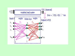
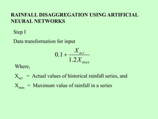
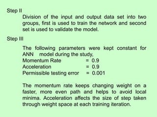
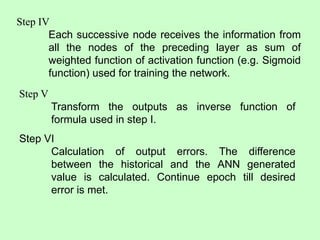
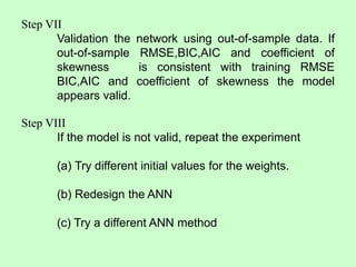
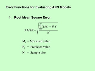
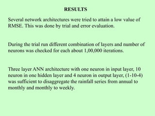
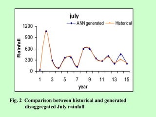
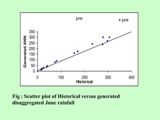
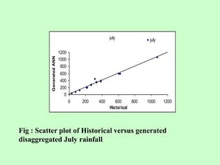
Rainfall Disaggregation modeling using stochastic model, Valencia-Schaake, Lane alongwith application of Artificial Neural Network to Disaggregate higher order scale time series to lower time scale series. ~Shashank Singh~

1. RAINFALL DISAGGREGATION USING ARTIFICIAL
NEURAL NETWORKS
Shashank Singh, R Subbaiah and H D Rank
College of Agricultural Engineering and
Technology,
Junagadh Agricultural University,
Junagadh 361 001
shashanksinghb4u@gmail.com

2. ARTIFICIAL NEURAL
NETWORKS
• Massively parallel distributed information
processing system resembling biological neural
networks of human brain
• First development in 1943 ( Mcculloch and Pitts)
• Engineering applications : signal processing,
robotics, control, hydrology, geotechnical
engineering to name a few

3. An average human brain has from 4 x 1010 to 1011
neurons. With the possibility of up to 104
interconnections per neuron, that enables 1015
interconnections (between neurons). A neuron is a
specialized cell for receiving, processing and
transmitting information by biochemical means
(neurotransmitters).
Structure of a biological neuron

4. ARTIFICIAL NEURON

5. MATHEMATICALLY
Transfer function- Sigmoid
Sum= ( X1W1+X2W2+ ….. ) + 
sum
e
1
1
Out 



7. OBJECTIVE
To disaggregate the annual rainfall series into
monthly rainfall series and monthly series to weekly
series using feed forward artificial neural network.

8. Rainfall Disaggregation
Disaggregation models are widely used tools for the
stochastic simulation of hydrologic series. They divide
known higher-level values (e.g. annual) into lower level ones
(e.g. seasonal), which add up to the given higher level. Thus
ability to transform a series from a higher time scale to a
lower one.

9. Mathematically
ε
B
AX
Y 

Valencia and Schaake Model (1972, 1973)
1

 xx
yx
S
S
A
xy
xx
yx
yy
t
S
S
S
S
BB 1



X is annual flow value and
Y is the column matrix containing the seasonal flow
values

10. RAINFALL DISAGGREGATION USING ARTIFICIAL
NEURAL NETWORKS
Data transformation for input
max
2
.
1
1
.
0
X
Xact

Where,
Xact = Actual values of historical rainfall series, and
Xmax = Maximum value of rainfall in a series
Step I

11. Step II
Division of the input and output data set into two
groups, first is used to train the network and second
set is used to validate the model.
Step III
The following parameters were kept constant for
ANN model during the study,
Momentum Rate = 0.9
Acceleration = 0.9
Permissible testing error = 0.001
The momentum rate keeps changing weight on a
faster, more even path and helps to avoid local
minima. Acceleration affects the size of step taken
through weight space at each training iteration.

12. Step IV
Each successive node receives the information from
all the nodes of the preceding layer as sum of
weighted function of activation function (e.g. Sigmoid
function) used for training the network.
Step V
Transform the outputs as inverse function of
formula used in step I.
Step VI
Calculation of output errors. The difference
between the historical and the ANN generated
value is calculated. Continue epoch till desired
error is met.

13. Step VII
Validation the network using out-of-sample data. If
out-of-sample RMSE,BIC,AIC and coefficient of
skewness is consistent with training RMSE
BIC,AIC and coefficient of skewness the model
appears valid.
Step VIII
If the model is not valid, repeat the experiment
(a) Try different initial values for the weights.
(b) Redesign the ANN
(c) Try a different ANN method

14. N
P
M
RMSE
N
t
t
t



 1
2
)
(
Mt = Measured value
Pt = Predicted value
N = Sample size
1. Root Mean Square Error
Error Functions for Evaluating ANN Models

15. N
N
n
RMSE
BIC
)
ln(
)
ln( 

N
n
RMSE
AIC
2
)
ln( 

n = Number of parameter estimated
N = Sample size
2. Bayesian information criteria (BIC)
3. Akaike information criterion (AIC)

16.          
X
X
X
X
M
X
X
M
i
i
3
1
3
2
3
3 









 

 

4. Coefficient of Skewness
Xi = Historical rainfall series.
  series
historical
of
Mean

X

  deviation
Standard

X


17. RESULTS
Several network architectures were tried to attain a low value of
RMSE. This was done by trial and error evaluation.
During the trial run different combination of layers and number of
neurons was checked for each about 1,00,000 iterations.
Three layer ANN architecture with one neuron in input layer, 10
neuron in one hidden layer and 4 neuron in output layer, (1-10-4)
was sufficient to disaggregate the rainfall series from annual to
monthly and monthly to weekly.

18. The generated monthly rainfall series are almost congruent
with the historical series (Fig 1). The scatter plot diagrams
between the ANN generated and historical monthly series
clearly showed that the generated values had values closer
to that of the historical values (Fig 2).

19. Table 1 RMSE, AIC, BIC values for ANN (1-10-4) generated
series four months
Season RMSE Skewness AIC BIC
June 13.826 2.253 3.8264 2.8583
July 37.244 3.861 4.2807 3.9366
August 34.306 2.162 4.1983 3.8472
September 6.9674 0.455 2.5993 2.1125

20. Season RMSE Skewness AIC BIC
Week 23 9.1428 1.226 2.8719 2.4082
Week 24 4.4545 2.05 2.1506 1.6257
Week 25 17.834 3.848 3.542 3.1352
Week 26 18.827 1.916 3.5964 3.1942
Week 27 43.138 1.591 4.428 4.0965
Week 28 28.134 1.691 3.9993 3.1364
Week 29 35.408 1.314 4.23 3.8816
Week 30 23.908 1.34 3.8361 3.4542
Week 31 10.48 2.053 3.008 2.5567
Week 32 9.6913 2.556 2.9303 2.4716
Week 33 24.104 2.499 3.8405 3.459
Week 34 41.042 3.869 4.3781 4.0423
Week 35 31.093 1.408 4.0996 3.7402
Week 36 12.856 2.542 3.2138 2.7791
Week 37 23.361 3.234 3.8128 3.429
Week 38 10.231 3.296 2.9847 2.5306
Week 39 10.351 2.107 2.9964 2.5433
Table 2 RMSE, AIC, BIC values for ANN (1-10-4)
generated series seventeen weeks

21. june
0
50
100
150
200
250
300
350
1 2 3 4 5 6 7 8 9 10 11 12 13 14 15
Years
Rainfall
Ann Generated
Historical
Fig. 1 Comparison between historical and generated
disaggregated June rainfall

22. july
0
300
600
900
1200
1 3 5 7 9 11 13 15
year
Rainfall
ANN generated Historical
Fig. 2 Comparison between historical and generated
disaggregated July rainfall

23. june
0
50
100
150
200
250
300
350
0 100 200 300 400
Historical
Generated
ANN
june
Fig : Scatter plot of Historical versus generated
disaggregated June rainfall

24. july
0
200
400
600
800
1000
1200
0 200 400 600 800 1000 1200
Historical
Generated
ANN
july
Fig : Scatter plot of Historical versus generated
disaggregated July rainfall