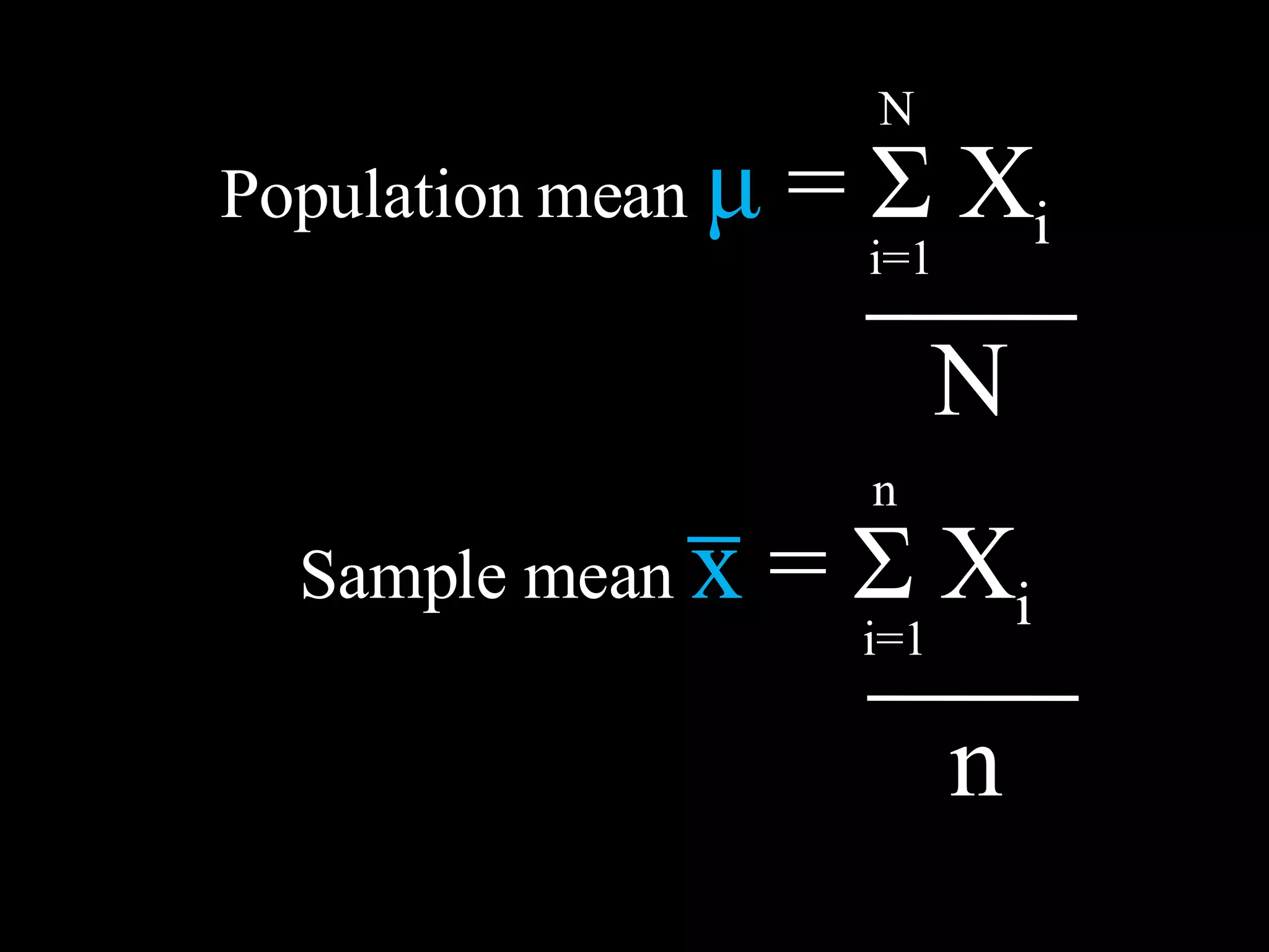
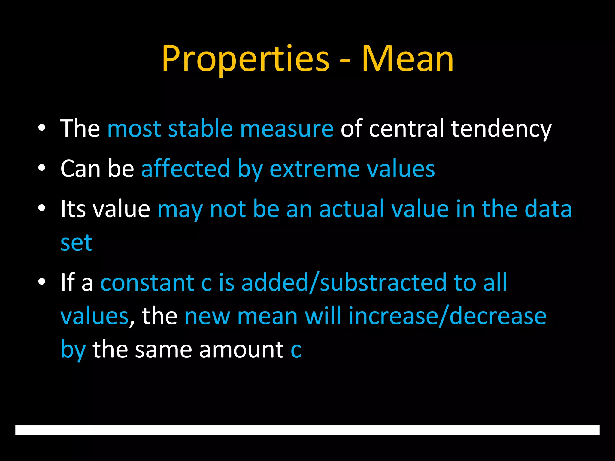
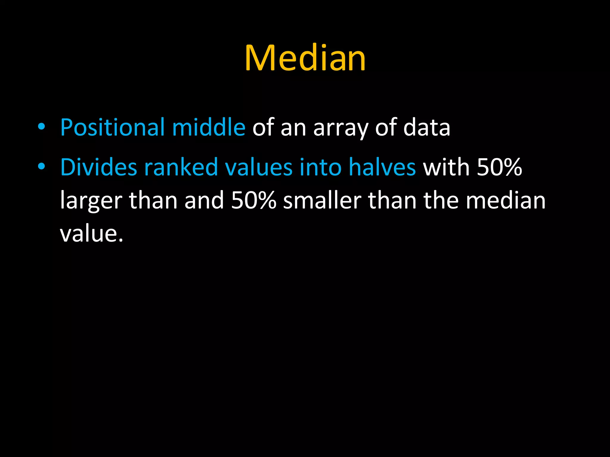
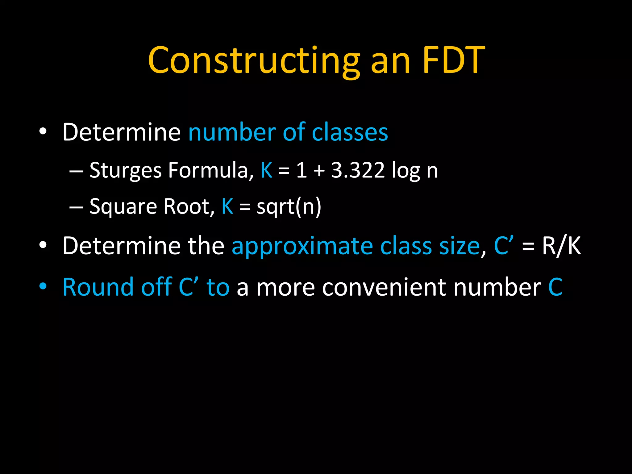
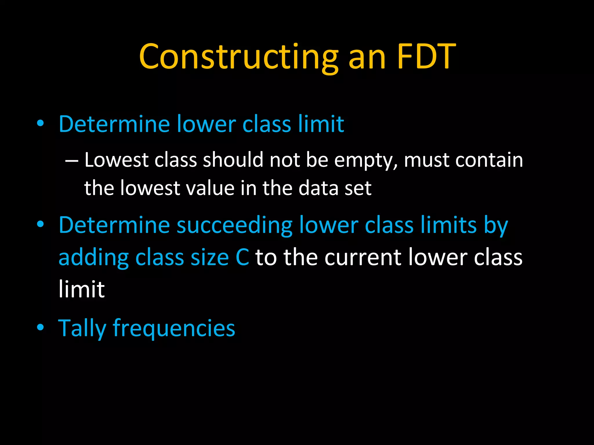
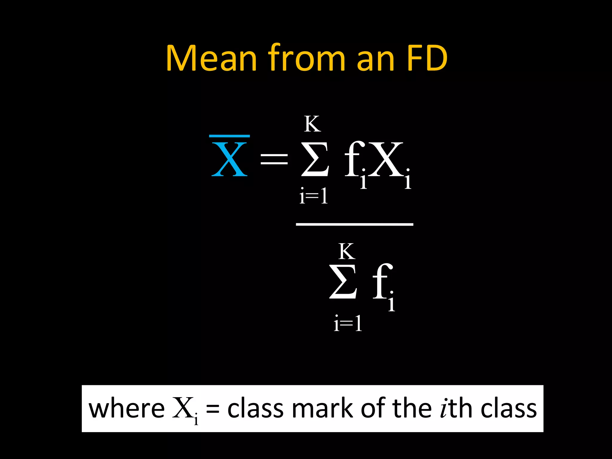
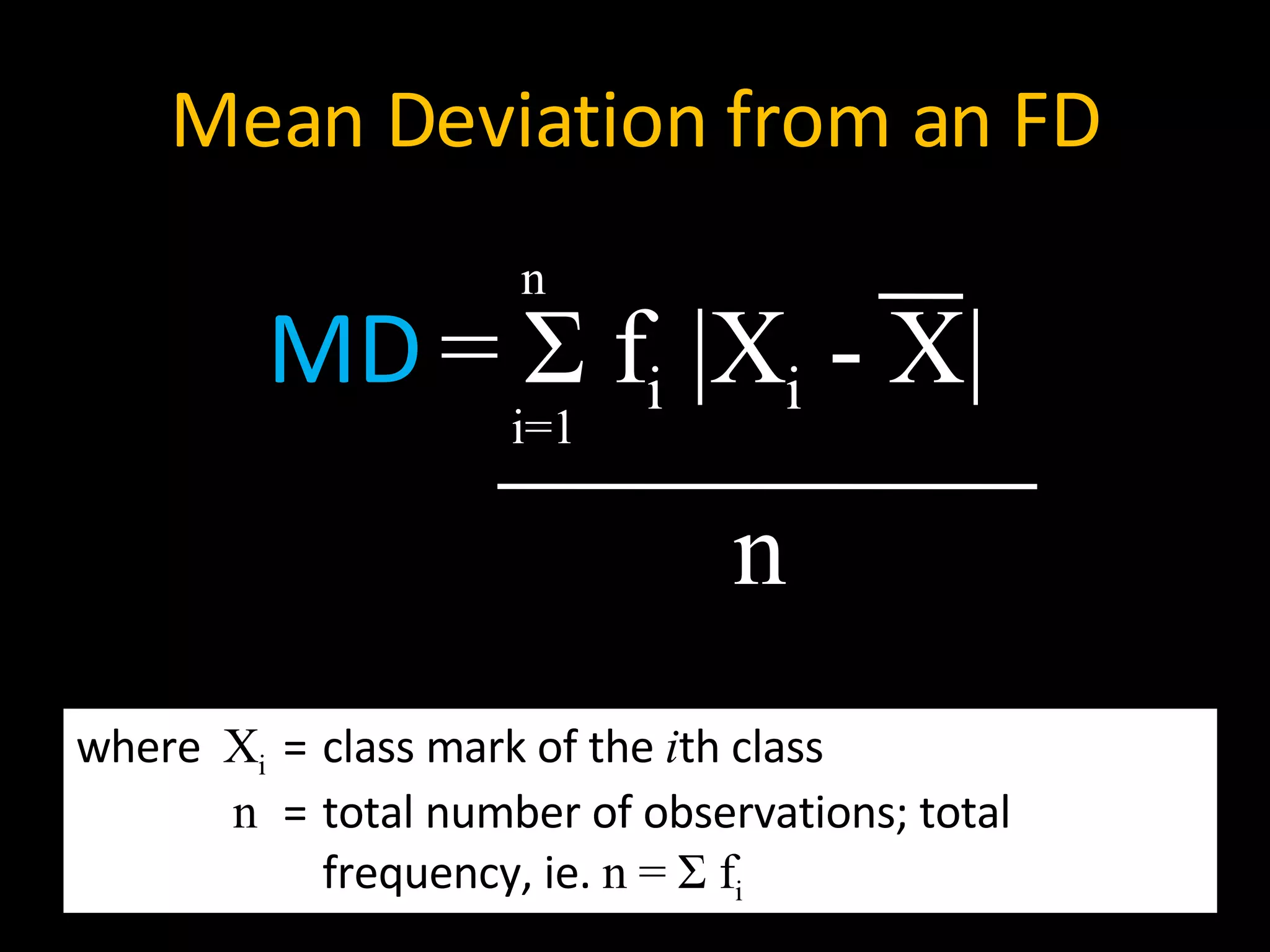
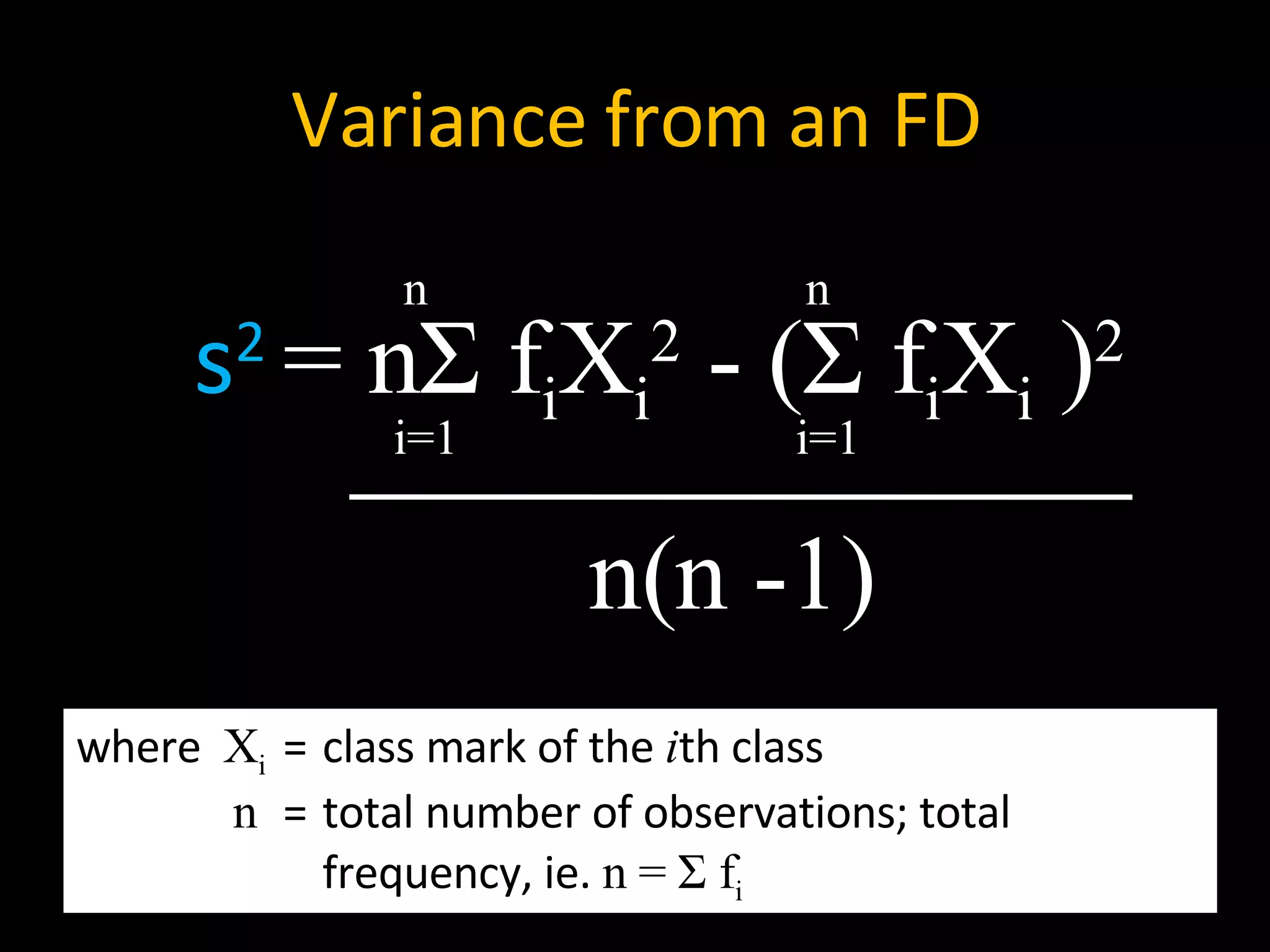
The document defines common statistical terms used to describe data distributions, including measures of central tendency (mean, median, mode), measures of variability (range, average deviation, variance, standard deviation), and how to construct a frequency distribution table from raw data by grouping values into classes and calculating frequencies. Key steps covered are determining the number of classes, class boundaries, frequencies, and how to find the mean, median, mode from the frequency distribution table.

1. Coverage Measures of Central Tendency Mean Median Mode Measures of Variability and Dispersion Range Average deviation Variance Standard deviation

2. Introduction to Notations If variable X is the variable of interest, and that n measurements are taken; then the notation X 1 , X 2 , X 3 , … , X n will be used to represent n observations .

3. Sigma Indicates “ summation of ” Σ

4. Summation Notation If variable X is the variable of interest, and that n measurements are taken; the sum of n observations can be written as Σ X i = X 1 +X 2 + … +X n n i=1

5. Summation Notation Σ X i = X 1 +X 2 + … +X n n i=1 Upper limit of summation Lower limit of summation Greek letter Sigma

6. Rules of Summation summation of the sum of variables is Σ (X i +Y i ) = Σ X i + Σ Y i n i=1 n i=1 n i=1 the sum of their summations

7. Σ (a i +b i +…+z i ) = Σ a i + Σ b i + … + Σ z i n i=1 n i=1 n i=1 n i=1 The summation of the sum of variables is… the sum of their summations .

8. Rules of Summation Σ cX i = c Σ X i = c(X 1 +X 2 + … +X n ) n i=1 n i=1 If c is a constant, then…

9. Rules of Summation Σ c = nc n i=1 The summation of a constant is the product of upper limit of summation n and constant c .

10. MEASURES OF CENTRAL TENDENCY Statistics in Research

11. Mean The sum of all values of the observations divided by the total number of observations The sum of all scores divided by the total frequency

12. Population mean μ = Σ X i N i=1 N Sample mean x = Σ X i n i=1 n

13. Mean in an Ungrouped Frequency Σ f i X i n i=1 n = (f 1 X 1 +f 2 X 2 + … +f n X n ) where f is the frequency of the occurring score n

14. Properties - Mean The most stable measure of central tendency Can be affected by extreme values Its value may not be an actual value in the data set If a constant c is added/substracted to all values , the new mean will increase/decrease by the same amount c

15. Median Positional middle of an array of data Divides ranked values into halves with 50% larger than and 50% smaller than the median value.

16. If n is odd : Md = X (n+1)/2 If n is even : Md = X n/2 + X (n/2)+1 2

17. Properties - Median The median is a positional measure Can be determined only if arranged in order Its value may not be an actual value in the data set It is affected by the position of items in the series but not by the value of each item Affected less by extreme values

18. Mode Value that occurs most frequently in the data set Locates the point where scores occur with the greatest density Less popular compared to mean and median measures

19. Properties - Mode It may not exist , or if it does, it may not be unique Not affected by extreme values Applicable for both qualitative and quantitative data

20. MEASURES OF VARIABILITY AND DISPERSION Statistics in Research

21. Range Measure of distance along the number line over where data exists Exclusive and inclusive range Exclusive range = largest score - smallest score Inclusive range = upper limit - lower limit

22. Properties - Range Rough and general measure of dispersion Largest and smallest extreme values determine the range Does not describe distribution of values within the upper and lower extremes Does not depend on number of data

23. Absolute Deviation Average of absolute deviations of scores from the mean ( Mean Deviation ) or the median ( Median Absolute Deviation )

24. MD = Σ | X i - X | n i=1 n MAD = Σ | X i - Md | n i=1 n

25. Properties – Absolute Deviation Measures variability of values in the data set Indicates how compact the group is on a certain measure

26. Variance Average of the square of deviations measured from the mean Population variance ( σ 2 ) and sample variance (s 2 )

27. σ 2 = Σ ( X i - μ ) 2 N i=1 N s 2 = Σ ( X i – X ) 2 n i=1 n -1

28. s 2 = n Σ X i 2 - ( Σ X i ) 2 n i=1 n(n -1) n i=1

29. Properties – Variance Addition/subtraction of a constant c to each score will not change the variance of the scores Multiplying each score by a constant c changes the variance, resulting in a new variance multiplied by c 2

30. Standard Deviation Square root of the average of the square of deviations measured from the mean – square root of the variance Population standard deviation ( σ ) and sample standard deviation (s)

31. σ = Σ ( X i - μ ) 2 N i=1 N s = Σ ( X i – X ) 2 n i=1 n -1

32. Why n-1? Degrees of freedom Measure of how much precision an estimate of variation has General rule is that the degrees of freedom decrease as more parameters have to be estimated Xbar estimates μ Using an estimated mean to find the standard deviation causes the loss of ONE degree of freedom

33. Properties – Standard Deviation Most used measure of variability Affected by every value of every observation Less affected by fluctuations and extreme values

34. Properties – Standard Deviation Addition/subtraction of a constant c to each score will not change the standard of the scores Multiplying each score by a constant c changes the standard deviation, resulting in a new standard deviation multiplied by c

35. Choosing a measure Range Data are too little or scattered to justify more precise and laborious measures Need to know only the total spread of scores Absolute Deviation Find and weigh deviations from the mean/median Extreme values unduly skews the standard deviation

36. Choosing a measure Standard Deviation Need a measure with the best stability Effect of extreme values have been deemed acceptable Compare and correlate with other data sets

37. FREQUENCY DISTRIBUTION Statistics in Research

38. Raw data 74 79 69 72 53 76 62 82 84 87 96 72 79 68 71 50 75 60 81 84 86 91 72 77 66 69 50 75 59 80 82 85 88 72 77 66 69 50 75 60 81 83 85 89 73 78 68 70 50 75 60 81 83 86 89 73 59 65 69 50 75 77 80 82 84 87 73 79 68 71 51 76 62 81 84 87 92 73 79 68 71 52 76 62 82 84 87 94 74 79 68 71 53 76 62 82 84 87 94 50 57 63 69 72 74 77 80 82 84 87

39. Array 50 57 63 69 72 74 77 80 82 84 87 50 59 65 69 72 75 77 80 82 84 87 50 59 66 69 72 75 77 80 82 85 88 50 60 66 69 72 75 77 81 83 85 89 50 60 68 70 73 75 78 81 83 86 89 50 60 68 71 73 75 79 81 84 86 91 51 62 68 71 73 76 79 81 84 87 92 52 62 68 71 73 76 79 82 84 87 94 53 62 68 71 74 76 79 82 84 87 94 53 62 69 72 74 76 79 82 84 87 96

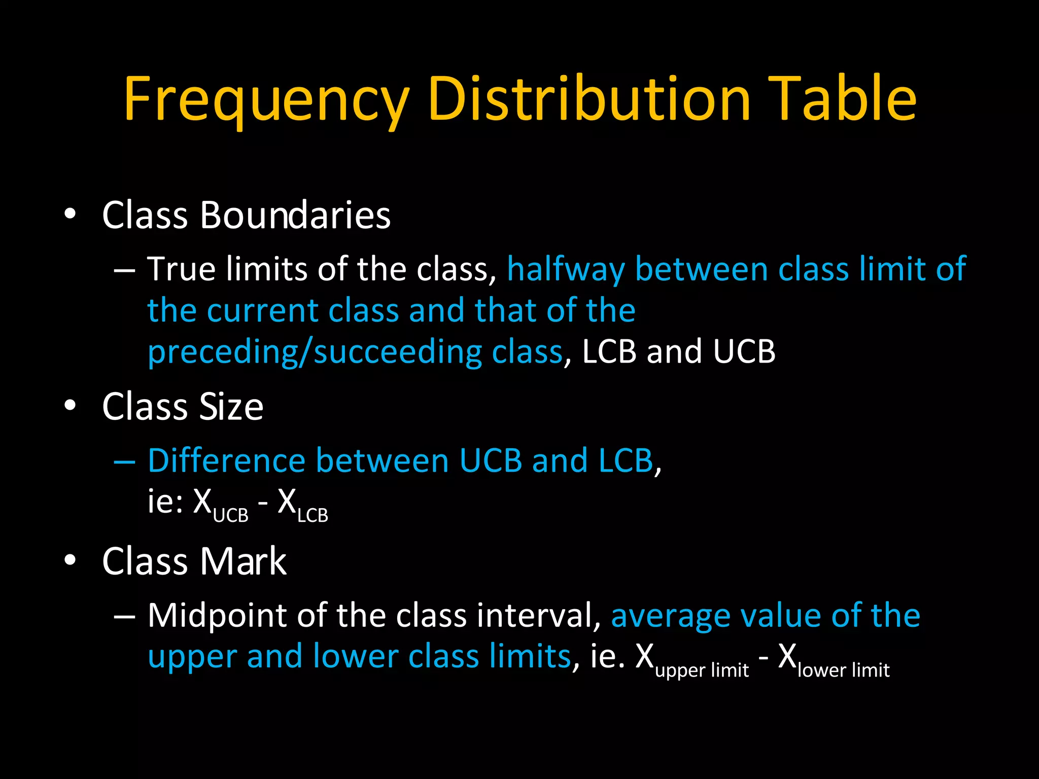
40. Frequency Distribution Table Class Frequency Number of observations within a class , f Class Limits End numbers of the class Class Interval Interval between the upper and lower class limits , ie: [X upper limit , X lower limit ]

41. Frequency Distribution Table Class Boundaries True limits of the class, halfway between class limit of the current class and that of the preceding/succeeding class , LCB and UCB Class Size Difference between UCB and LCB , ie: X UCB - X LCB Class Mark Midpoint of the class interval, average value of the upper and lower class limits , ie. X upper limit - X lower limit

42. Constructing an FDT Determine number of classes Sturges Formula, K = 1 + 3.322 log n Square Root, K = sqrt(n) Determine the approximate class size , C’ = R/K Round off C’ to a more convenient number C

43. Constructing an FDT Determine lower class limit Lowest class should not be empty, must contain the lowest value in the data set Determine succeeding lower class limits by adding class size C to the current lower class limit Tally frequencies

44. Array 50 57 63 69 72 74 77 80 82 84 87 50 59 65 69 72 75 77 80 82 84 87 50 59 66 69 72 75 77 80 82 85 88 50 60 66 69 72 75 77 81 83 85 89 50 60 68 70 73 75 78 81 83 86 89 50 60 68 71 73 75 79 81 84 86 91 51 62 68 71 73 76 79 81 84 87 92 52 62 68 71 73 76 79 82 84 87 94 53 62 68 71 74 76 79 82 84 87 94 53 62 69 72 74 76 79 82 84 87 96

45. Frequency Distribution Table Class Frequency LCB UCB RF <CF >CF 50-54 10 49.5 54.5 0.09 10 110 55-59 3 54.5 59.5 0.03 13 100 60-64 8 59.5 64.5 0.07 21 97 65-69 13 64.5 69.5 0.12 34 89 70-74 17 69.5 74.5 0.15 51 76 75-79 19 74.5 79.5 0.17 70 59 80-84 22 79.5 84.5 0.20 92 40 85-89 13 84.5 89.5 0.12 105 18 90-94 4 89.5 94.5 0.04 109 5 95-99 1 94.5 99.5 0.01 110 1

46. Other Terms Relative frequency, RF Class frequency divided by number of observations , ie. RF = f i / n Relative Frequency Percentage, RFP RF = (f i / n) x 100% Cummulative frequency Shows accumulated frequencies of successive classes , either from the beginning (less than CF) or end (greater than CF) of the FDT

47. Mean from an FD X = Σ f i X i K i=1 Σ f i K i=1 where X i = class mark of the i th class

48. Median from an FD Md = LCB Md + C n/2 - <CF Md-1 where LCB Md = lower class boundary of median class <CF Md-1 = less than cumulative frequency preceeding the median class f Md

49. Mode from an FD Mo = LCB Mo + C f Mo - f Mo-1 where LCB Mo = lower class boundary of modal class f Mo , f Mo-1 , f Mo+1 = frequency of modal class, class preceding and class succeeding the modal class 2f Mo - f Mo-1 - f Mo+1

50. Mean Deviation from an FD MD = Σ f i |X i - X| n i=1 n where X i = class mark of the i th class n = total number of observations; total frequency, ie. n = Σ f i

51. Variance from an FD s 2 = Σ f i (X i - X) 2 n i=1 (n -1) where X i = class mark of the i th class n = total number of observations; total frequency, ie. n = Σ f i

52. Variance from an FD s 2 = n Σ f i X i 2 - ( Σ f i X i ) 2 n i=1 n(n -1) n i=1 where X i = class mark of the i th class n = total number of observations; total frequency, ie. n = Σ f i