Group1_Descriptive Statictis and Data Presentation.pdf

DESCRIPTIVE STATISTICS
AND DATA PRESENTATION
DESCRIPTIVE STATISTICS
AND DATA PRESENTATION
ANALISIS DATA
BY GROUP 1

GROUP 1
GROUP 1
Tari Agustin
25021340008
Karina Septiani
25021340011
Andika Guruh S.
25021340017
M. Dani Andhika P.
25021340018

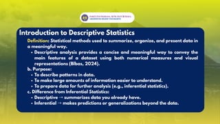
Introduction to Descriptive Statistics
Definition: Statistical methods used to summarize, organize, and present data in
a meaningful way.
Descriptive analysis provides a concise and meaningful way to convey the
main features of a dataset using both numerical measures and visual
representations (Blbas, 2024).
b. Purpose:
To describe patterns in data.
To make large amounts of information easier to understand.
To prepare data for further analysis (e.g., inferential statistics).
c. Difference from Inferential Statistics:
Descriptive →summarizes data you already have.
Inferential →makes predictions or generalizations beyond the data.

Organizing Data and Graphing Data
It is essential to create frequency distributions to facilitate researchers in
describing, summarizing, and reporting their data.
a. Frequency Distributions
A frequency distribution is a data presentation tool in the form of
columns and rows (tables), which contains numbers that depict the
frequency distribution of the variables being studied.

Example:
Table 1. Scores of Twenty-five
Students on a Thirty-item Social
Studies Test
Table 2. A Frequency Distribution of a Thirty-
item Test Ordered from the Highest to the
Lowest Score: Test Scores of Twenty-five
Students

Various types of frequency distributions
Single Data Frequency Distribution
Single data frequency distribution is the
distribution of numerical data
without grouping the variable values
(ungrouped data).
Group Data Frequency Distribution
Group Data Frequency Distributionis a presentation
of data from variable values that are large or
varied, to facilitate analysis and presentation.
Steps:
1. Determine the range
Range = Largest data – smallest data
2. Determine the number of interval classes using Sturges' formula
Number of classes = 1 +(3.3) log n
3. Determine the length of the interval class (p) using the following
formula:
p = n/range

Various types of frequency distributions
Absolute frequency distribution is a number that
indicates the amount of data in a particular group.
Absolute Frequency Distribution Relative Frequency Distribution
A relative frequency distribution is a percentage that
indicates the amount of data in a particular group.

Class Intervals
Class Interval is a range of values into which data is grouped for the purpose
of organizing, summarizing, and analyzing data efficiently.
When we have many scores (20 or more), it is better to put them into
groups.
These groups are called class intervals (e.g., 20–25, 26–30).
Problem: We lose details → if 4 students are in 20–25, we don’t know their
exact scores.

Rules for Class Intervals
All intervals must be the same size.
A score can be in only one interval, not two.
Better to use an odd number (5, 7, 9) →midpoint is a whole number.

Cumulative Frequency Distribution
A cumulative frequency distribution shows the total number of data values that
fall at or below a certain point.
It is useful for finding how many values are below or above a specific score.
A cumulative frequency table usually includes:
Score / Class Interval →the data values
Frequency →how often each value occurs
Percent Frequency →frequency as a percentage
Cumulative Frequency →running total of frequencies
Cumulative Percentage →running total in percentages

Graphing Data
a. Histogram - Helps identify
gaps in data.
b. Frequency polygon - Easier to
compare multiple distributions on the
same graph

Graphing Data
c. Pie Graph - Visually intuitive for
showing percentages.
d. Bar Graph - Works well for
continuous data and comparisons

Graphing Data
e. Line Graph - Highlights
increases, decreases, and
fluctuations
f. Box Plot (box and whiskers) - Shows
the spread and decrease or increase of
a group of data.

Graphing Data
g. Comparing Histograms and
Frequency Polygons

Measures of Central Tendency
A measure of central tendency is a summary score
that represents a set of scores. (Ravid Ruth, 2011)
Mode
Definition: The mode of a
distribution is the score that
occurs with the greatest
frequency in that distribution.
Example :

Median
Definition: The middle value when a set of data values has been ordered
from lowest to highest value.
Example:
Suppose we have the following set of 6 scores:
Scores: 10, 12, 13, 13, 15, 16
Step 1: Arrange the scores in order (already done)
Step 2: Count the number of scores
Step 3: Find the middle two scores
Step 4: Calculate the median

Mean
Definition: The mean, which is also called the arithmetic mean, is obtained by
adding up the scores and dividing that sum by the number of scores. The
mean is sometimes called the arithmetic mean and the average.
Formula for the Mean:
Mean :
Example:
Suppose we have the following test scores:
70, 80, 85, 90, 95
Step 1: Add all the values
Step 2: Count the number of values
Step 3: Apply the formula

Measures of
Central Tendency
Comparing the Mode,
Median, and Mean

Measures of Variability
The Range
Range is the difference between the highest and lowest values in a dataset. It
gives a quick sense of how spread out the numbers are.
Example: You have data 2, 4, 4, 6, 10 →Range = 10 − 2 = 8
Strengths: Easy to compute.
Weaknesses: Based only on 2 values →highly affected by outliers.
Standard Deviation and Variance
a. The deviation score is the distance of the raw score from the mean,
indicated by X – X– (i.e., the score minus the mean). The sum of the deviation
scores (i.e., the distances between the raw scores and the mean of that
distribution) is always 0 (zero).

b. The variance is the mean of the squared deviations. To calculate it, square
each deviation score, add all the squared deviations, and divide their sum by
n – 1 (the number of scores minus 1) for the sample variance.

a. Step 1: Find the mean (average)
Add them: 2 + 4 + 6 = 12
Divide by (n) 3 →mean = 4
b. Step 2: Find the deviation (difference from the mean)
2 − 4 = −2
4 − 4 = 0
6 − 4 = +2
So deviations are: −2, 0, +2
c. Step 3: Square the deviations (to remove minus)
(−2)² = 4
0² = 0
(+2)² = 4
So squared deviations: 4, 0, 4

Step 4: Find the variance
Add them: 4 + 0 + 4 = 8
If we use population variance (all data included) →divide by 3 →8 ÷ 3 = 2.67
If we use sample variance (just a small part of bigger data) → divide by (3 −
1) = 2 →8 ÷ 2 = 4
Step 5: Find the standard deviation (the square root of variance)
Population SD = √2.67 ≈1.63
Sample SD = √4 = 2
✅Simple rule:
If you have all the data →use divide by n (population).
If you only have a sample from a bigger population → use divide by n − 1
(sample).

Computing the Variance and SD for Populations and Samples
1.Population: When you have all the data (the whole group), divide by N
(the number of scores).
2.Sample: When you only have part of the group (a sample), divide by n-1.
This adjustment (called Bessel’s correction) makes the result more
accurate.
3.Steps (conceptual, no formula):
a.Find the mean.
b.See how far each score is from the mean (deviation).
c.Square those deviations (to avoid negatives).
d.Average them →this is variance.
e.Take the square root →this is standard deviation (SD).

Using the Variance and SD
1.Variance and SD show how spread out the data is.
2.Small SD = scores are close to the mean (less variation).
3.Big SD = scores are spread out (more variation).
4.Uses in research:
To compare two groups (which group is more consistent?).
To understand reliability (stable or unstable scores?).
To identify how much individual scores differ from the average

Variance and SD in Distributions with Extreme Scores
1.Extreme scores (outliers) increase the variance and SD a lot.
2.Example: if most students score 80–90, but one student scores 20, the SD
becomes much larger.
3.That’s why researchers check data for outliers before analysis.

Factors Affecting the Variance and SD
1.Range of scores – wider range = bigger SD.
2.Mean differences – scores clustered near
the mean = smaller SD.
3.Outliers – extreme values increase SD.
4.Sample size – smaller samples tend to have
more unstable SD; bigger samples give a
more reliable SD.

THANKS FOR YOUR KIND ATTENTION
DISCUSSION SEASON

Group1_Descriptive Statictis and Data Presentation.pdf

More Related Content

Similar to Group1_Descriptive Statictis and Data Presentation.pdf

Recently uploaded

Group1_Descriptive Statictis and Data Presentation.pdf