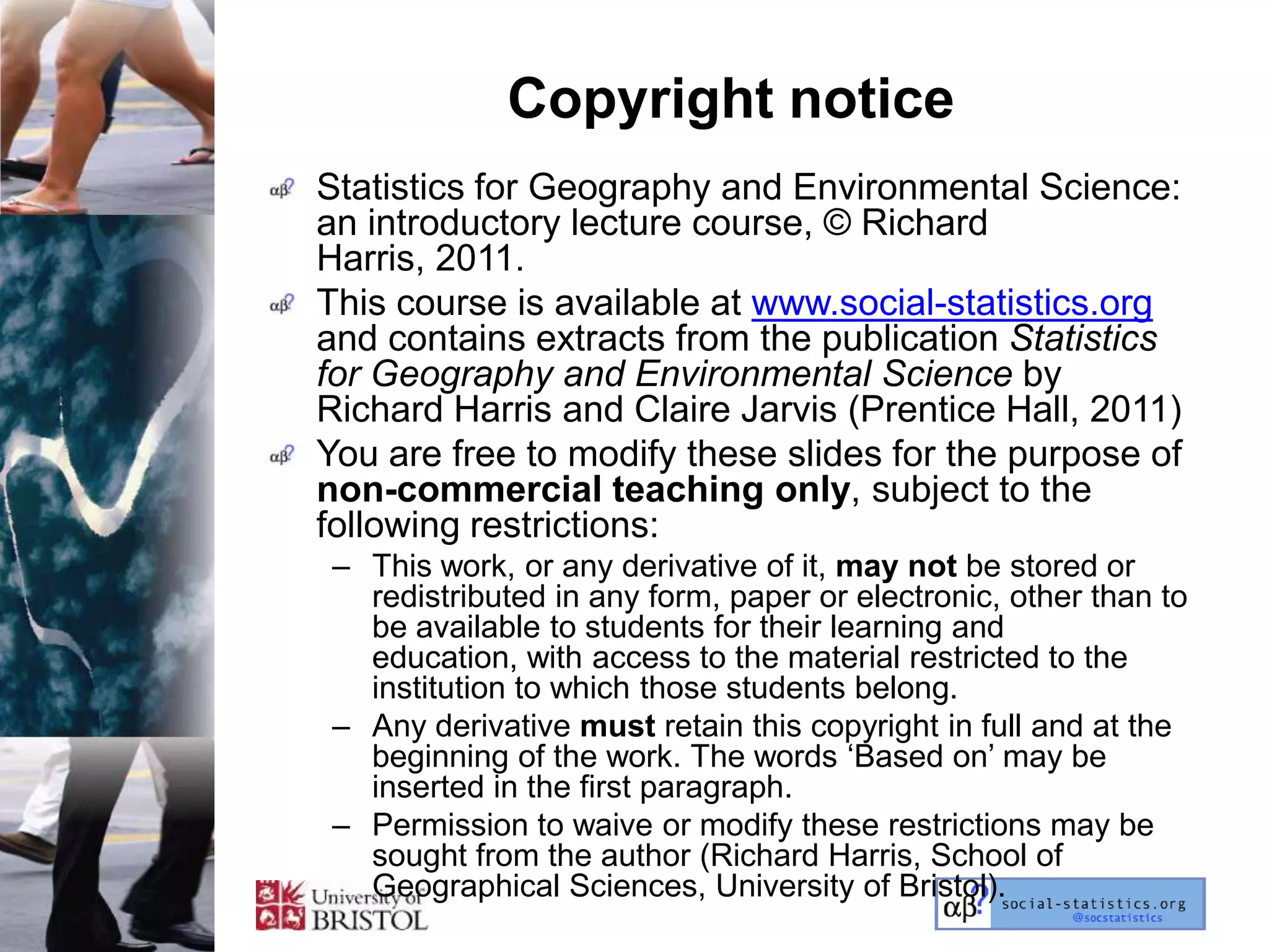
Statistics for Geography and Environmental Science:an introductory lecture course

Statistics for Geography and
Environmental Science:
an introductory lecture course
By Richard Harris, with material
by Claire Jarvis
USA: http://amzn.to/rNBWd5
UK: http://amzn.to/tZ7fVu

Copyright notice
Statistics for Geography and Environmental Science:
an introductory lecture course, © Richard
Harris, 2011.
This course is available at www.social-statistics.org
and contains extracts from the publication Statistics
for Geography and Environmental Science by
Richard Harris and Claire Jarvis (Prentice Hall, 2011)
You are free to modify these slides for the purpose of
non-commercial teaching only, subject to the
following restrictions:
– This work, or any derivative of it, may not be stored or
redistributed in any form, paper or electronic, other than to
be available to students for their learning and
education, with access to the material restricted to the
institution to which those students belong.
– Any derivative must retain this copyright in full and at the
beginning of the work. The words ‗Based on‘ may be
inserted in the first paragraph.
– Permission to waive or modify these restrictions may be
sought from the author (Richard Harris, School of
Geographical Sciences, University of Bristol).

The modules

Module1 makes the case for knowing
about statistics as a transferable skill
and to be equipped for social and
political debate.
Module 2 is about using descriptive
statistics and simple graphical
techniques to explore and make
sense of data.
Module 3 discusses the Normal
curve, the properties of which
provide the basis for inferential

The modules

Module 4 is about the principles of
research design and effective data
collection.
Module 6 discusses the role of
hypothesis testing.
Module 7 is about regression
analysis.

The modules

Module 8 moves to modelling point
patterns, ―hotspot analysis‖ and ways
of measuring patterns of spatial
autocorrelation in data.
Module 9 looks at spatial regression
models, geographically weighted
regression and multilevel modelling.
Each module is explored more fully
in the accompanying
textbook, Statistics for Geography
and Environmental Science.

Module 1
(Extracts from Chapter 1 of Statistics for Geography
and Environmental Science)

DATA, STATISTICS AND
GEOGRAPHY

Module overview

To convince you that studying
statistics is a good idea!
Our argument is that data collection
and analysis are central to the
functioning of contemporary society
so knowledge of quantitative
methods is a necessary skill to
contribute to social and scientific
debate.

About statistics

Statistics are a reflective practice: a
way of approaching research that
requires a clear and manageable
research question to be formulated, a
means to answer that question,
knowledge of the assumptions of
each test used, an understanding of
the consequences of violating those
assumptions, and awareness of the
researcher‘s own prejudices when
doing the research.

Some reasons to study statistics

Reasons for human geographers
– Data collection and analysis are central
to the functioning of society, to systems
of governance and science.
– Knowledge of statistics is an entry into
debate, informed critique and the
possibility of creating change.


Reasons for GI scientists
– To address the uncertainties and
ambiguities of using data analytical.
– Because of the increased integration of
mapping capabilities, data visualizations
and (geo-) statistical analysis.


Reasons for all students
– They provide a transferable skill set
using in other areas of research, study
and employment.
– There is a recognised shortage of
students with skills in quantitative
methods, especially within the social
sciences.

Types of statistic

Descriptive
– Used to provide a summary of a set of
measurements, e.g. the average.
Inferential
– Use the data at hand to convey information
about the population (‗the greater
something‘) from which the data are drawn.
Relational
– Consider whether greater or lesser values
in one set of data are related to greater or
lesser values in another.

Geographical data

These are records of what has
happened at some location on the
Earth‘s surface and where.
For many statistical tests the where
is largely ignored.
However, it is central to geostatistics
and to spatial statistics (as their
names suggest)

Some problems when analysing
geographical data

Standard statistical tests assume that
each ‗bit‘ of data (each observation)
has a value that is not influenced by
any other.
However, we may often expect there
to be geographical patterns in the
data.
– Spatial autocorrelation: geographical
patterns in the measurements

geographical data

Determining what causes what in a
complex and dynamic natural or
social system is extremely tricky.
Two things may be associated (e.g.
greater income inequality and more
non-recycled waste) without the one
directly causing the other.

geographical data

Data and structured forms of enquiry
can only tell us so much and may not
be appropriate to some types of
research for which a more
qualitative, participatory or less
representational approach may be
better.

Further reading

Chapter 1 of Statistics for
Geography and Environmental
Science by Richard Harris and Claire
Jarvis (Prentice Hall / Pearson, 2011)
Includes a review of the following
key concepts: types of statistics;
why error is unavoidable;
geographical data analysis; and
spatial autocorrelation and the first
law of geography.

Module 2

DESCRIPTIVE STATISTICS

Module overview

This module is about ―everyday
statistics‖, the sort that summarise
data and describe them in simple
ways.
They include the number of home
runs this season, average male
earnings, numbers unemployed,
outside temperature, average cost of
a barrel of oil, regional variations in
crime rates, pollution statistics,
measures of the economy and other
―facts and figures‖

Data and variables

Data
– A collection of observations:
measurements made of something.
A variable
– Another name for a collection of data.
Variable because it is unlikely that the
data are all the same.
Data types
– These include
discrete, continuous, and categorical
data.

Simple ways of presenting data

Discrete data Continuous data
Frequency table Summary table
Bar chart (below) Histogram (below, with a rug plot)

Information to include
in a summary table

Measures of central tendency
(―averages‖)
– The mean and/or median
• The ―centre‖ of the data
Measures of spread and variation
– The range (minimum to maximum)
– The interquartile range (from ‗mid-
spread‘ of the data)
– The standard deviation,s

More about the standard deviation

Essentially a measure of average
variation around the mean.
It is also the square root of the
variance.
The variance is the sum of squares
divided by the degrees of freedom

Boxplots

Are useful for
showing the
median,
interquartile
range and range
of a set of data,
for indentifying
outliers and also
for comparing
variables.

Other ways of classifying numeric
data

Nominal, ordinal, interval and ratio
Counts and rates
Proportions and percentages
Parametric and non—parametric
Arithmetic and geometric
Primary and secondary

Further reading

Chapter 2 of Statistics for Geography
and Environmental Science by Richard
Harris and Claire Jarvis (Prentice Hall /
Pearson, 2011)
Includes a review of the following key
concepts: data and variables; discrete
and continuous data; the range;
histograms, rug plots, and stem and
leaf plots; measures of central
tendency; why averages can be
misleading; quantiles; the sum of
squares; degrees of freedom; the
standard deviation and the variance;
box plots; and five and six number
summaries

Module 3

THE NORMAL CURVE

Module overview

This module introduces the normal
curve, so called because it is how
many social and scientific data
appear distributed.

The normal curve

It is also known as
the Gaussian
distribution and is
often described as
‗bell-shaped‘
It is a family of
distributions all of
which have the
same probability
density function
(the same formula
defining their
shape).

The central limit theorem

The central limit theorem states that
the sum (and therefore average) of a
large number of independent and
identically distributed random
variables will approach a normal
distribution as the sample size
increases, even if the variables are
not themselves normally distributed.

Properties of a normal curve

Ranges from
negative to positive
infinity
Is symmetrical
around its mean
95% of the area
under the curve is
within 1.96
standard
deviations of the
mean
99% of the area is
within 2.58
standard
deviations.

Properties of a normal curve

Consequently, if a
data set is
approximately
Normal, the
probability of
selecting, at random,
an observation at
that is within 1.96
standard deviations
of the mean is p =
0.95, and the
probability it will be
within 2.58 standard
deviations is p
=0.99.

Standardising data (z values)

Data are
standardised if their
original
measurement units
are replaced with
units of standard
deviation from the
mean (z values).
It is a little like
converting a
proportion (0 to 1) to
a percentage (0 to
100): it doesn‘t
change the shape of
the data.

Standardising data (z values)

The z values are calculated by
subtracting the mean of the data from
each observation and then dividing by
the standard deviation.
Once data are standardised and
assuming they are approximately
normal then they can be compared
against the Standard Normal curve.
This is a special instance of a normal
curve that has a mean of zero and a
standard deviation of one.
It provides a model or benchmark for
the data.

Probability and the Standard
Normal

The area between two z values
(under the Standard Normal) is the
probability of selecting an
observation randomly from the data
that will have a z value between
those two values.
That area can be determined using a
statistical table or equivalent.

Probability and the Standard
Normal

See the worked
examples on pp.
62–70 of
Statistics for
Geography and
Environmental
Science

Some data are skewed but can
often be transformed to
approximate normality

The quantile plot

Useful (and better
than a histogram)
to check for non-
normality, such as
skew and the
presence of
outliers.
If the data were
normal they‘d be
distributed along
the straight line.

Further reading

Pearson, 2011)
concepts: properties of normal curves;
the central limit theorem; probability
and the normal curve; finding the area
under the normal curve; skewed data
and the ‗ladder of transformation‘;
moments of a distribution; and the
quantile plot.

Module 4

SAMPLING

Module overview

It is rarely possible or necessary to
collect all possible data about
something that is being studied.
This module is about how to go
about collecting a sample of data that
is fit for a particular research task.

Sampling

It is common in geographical and
other research to gather a sample
(or subset) of data from a target
population.
The aim is for the sample to be
representative of that population.
Sampling bias occurs when the
sample favour some parts of the
target population more than
others, perhaps by sampling at an
unrepresentative time or place or
because of the data collection

The process of sampling

Define the research question
Review the related literature
Review the scope of the planned
study
Construct a sample frame
Select a sample design method
Review the design from
practical, ethical, safety and logistical
perspectives
Implement the design and collect the

Sampling methods

Sampling methods

Non-probabilistic Probabilistic sampling
sampling methods methods

Judgemental Convenience Simple Systematic
random

Quota Snowball Clustered Stratified
random random

Sampling methods

The different methods are outlined on pp.
94-105 of Statistics for Geography and
Environmental Science.
In general, random sampling methods are
preferred because the errors in the data
should be random too.
However, a random sample won‘t
necessarily offer a wide enough coverage
of the target population.
Therefore stratified samples may be used
which may themselves target
specific, representative places to reduce
the cost and ease the logistics of the data
collection.

Sampling error and sample size

The impression that is formed of the target
population depends on the sample of data
taken to represent it.
It is possible that a random sample
accidentally misrepresents the population
if it happens only to observe its most
unusual occurrences: it is susceptible to
sampling error.
The larger the sample (the more
observations there are) there smaller the
error is expected to be but with
‗diminishing returns‘
– the error is generally proportional to the square
root of the sample size

Sampling error and sample size

The error is also a function of how
much the target population varies
– If it were exactly the same, everywhere, it
wouldn‘t matter where the samples were
taken
A larger sample is costly and more time
consuming to collect.
However, a small sample of a highly
variable population is unlikely to
generate any statistically meaningful
analytical results.

Sampling methods: issues and
practicalities

Personal safety, gaining permission
from an ethics committee, what to do
about missing data.
Practical considerations
– Weight and/or volume of the
sample, import/export
restrictions, analytical costs
Instrument accuracy and scale
Bottom line: if your sample is no
good, your analysis won‘t be any
good either.

Further reading

Pearson, 2011)
concepts: the target population;
representative samples; sampling
frames; sampling bias; metadata;
fitness for purpose and use; sample
design; sampling error and sample size;
sample size and replicates; and
measurement accuracy.

Module 5

FROM DESCRIPTION TO
INFERENCE

Module overview

This module is about inference.
Inference is at the heart of how and
why statistics developed.
It moves beyond simply summarising
data (the sample) to using those
summaries to gain insights into the
underlying system, process or
structure that the data are
measurements of (the population).

A population

Its meaning isn‘t restricted to ―everyone
who lives in a particular place‖ but can
be much more abstract.
– ―Every possible object (or entity) from which
the sample is selected.‖
– ―The complete set of all possible
measurements that might hypothetically be
recorded.‖
Informally: the complete ‗thing‘ that you
are interested in study but which can‘t
be measured in its entirety.

Each sample changes our
impression of the population

The sample mean and
the population mean

Assuming the sample is
representative (unbiased), it is
possible to estimate the true mean of
the population from the mean for the
sample.
– The population mean from the sample
mean
But that estimate is sample
dependent
– Change the sample and you get a
different estimate

Confidence intervals

It is improbable that the sample
mean is exactly equal to the
population mean
– And we wouldn‘t know even if it was.
• (unless we sampled the population in its
entirety, in which case they‘d be no need to
make an estimate!)
However, we can place a confidence
interval around the sample mean and
estimate the probability that
confidence interval contains the
population mean.

The width of a confidence interval

The confidence interval is wider
– The greater the probability you want it to
contain the unknown population mean
– The more variable the data are (the
greater their variance / standard
deviation)
– The less data you have

The standard error (of the mean)

The standard deviation of the data
divided by the square root of the
number of observations gives an
estimate of the standard error (of
the mean) and is a measure of
uncertainty in the data
– The greater the standard error, the
greater the uncertainty

Why confidence intervals ‘work’

In principle, if a
population were
sampled a very large
number of times, the
sample mean
calculated in each
case and those means
then collected together
to form a new
variable, we‘d find that
variable to be normally
distributed, centred on
the population mean
and with a standard
deviation equal to the
standard error of the
mean.

Small samples

For small samples the
confidence interval will
be underestimated if it is
calculated with reference
to a normal distribution.
A t-distribution is used
instead.
This is ‗fatter‘ than the
normal.
Intuitively: we are more
cautious with small
samples that contain little
information. The
confidence intervals are
widened to reflect that
caution.

Summary

Mean of the sample Known
Standard deviation of the sample Known
Standard deviation of the Unknown but approximated by
population the standard deviation of the
sample
Standard error of the mean Estimated as the standard
deviation of the sample divided by
the square root of the sample size
Mean of the population Unknown but we can estimate the
probability that it has a value that
lies within a given number of
standard errors either side of the
sample mean (within a given
confidence interval)

Further reading

key concepts: inference, samples
and populations; the distribution of
the sample means; standard error of
the mean; confidence intervals; the t-
distribution and confidence intervals
for ‗small samples‘

Module 6

HYPOTHESIS TESTING

Module overview

This module introduces hypothesis
testing as a way of formally
questioning whether a population
mean could plausibly be equal to a
hypothesised value, and to consider
whether two or more samples of data
were most probably drawn from the
same population.

The process of hypothesis testing

Define the null hypothesis
Define the alternative hypothesis
Specify an alpha value
– The maximum probability of rejecting the
null hypothesis when it is, in fact, correct.
Calculate the test statistic
Compare the test statistic with a critical
value
Reject the null hypothesis is the test
statistic has greater magnitude than the
critical value

One-sample t test

The one-sample t test measures the
number of standard errors the sample
mean is from an hypothesised value.
The further it is, the less probably the
sample is drawn from a population with a
mean equal to that hypothesised value.
The p value records that probability.
A p value of 0.95 or greater means we can
be (at least) ―95% confident‖ that the ―true
mean‖ (the population mean) for whatever
has been measured is not the
hypothesised value.
A p value of 0.99 or greater gives 99%
confidence

Two-sample t test

Considers the probability that two samples
of data do not have the same population
mean.
– If they don‘t, it suggests the samples measure
categorically different things.
It works by measuring the difference
between the sample means relative to the
variance of the samples.
There are different versions of the t
test, for example for paired data and for
whether the two samples have
approximately equal variance or not.
An F test is used to compare the sample
variances and see if any difference could
be due to chance.

Analysis of variance (ANOVA)

Used to test whether
three or more groups
of data have the
same population
mean.
Considers the
variations between
groups relative to the
variation within
groups.
Contrasts can be
used to specifically
contrast one or more
of the groups with
one or more of the

Two- and one-tailed tests

A two-tailed test is
non-directional
whereas a one-tailed
test is directional.
Consider a one-
sample t test
– The alternative
hypothesis for a two-
tailed test is only that
the population mean
is not equal to the
hypothesised value.
– A one-tailed test it
specifies which is the
greater

Non-parametric tests

Non-parametric
tests do not begin Parametric Non-
with fixed parametric
assumptions about Two-samplet Wilcoxon rank
how the data and test sum test (aka
Mann-Whitney
the population are test)
distributed ANOVA Kruskal-Wallis
– E.g. a normal test
distribution
However, if the
assumptions are
met, it is better to
use the parametric
test.

Possible outcomes of a statistical
test

Power

We worry about limiting the probability of
rejecting the null hypothesis when it is
correct (of making a wrong decision)
– Of having a low p value
But we could avoid the error by never
rejecting the null hypothesis
Except, that‘s daft because the null
hypothesis could be wrong.
So, also need to think about the probability
of rejecting the null hypothesis when it is
indeed wrong
– The probability of making this, the right
decision, is the power of the test.

Further reading

Pearson, 2011)
concepts: type I errors; the one-
sample t test; hypothesis testing; two-
and one-tailed tests; type II errors and
statistical power;
homoscedasticity, heteroscedasticity
and the F test; analysis of variance;
measuring effects; and parametric and
non-parametric tests.

Module 7

RELATIONSHIPS AND
EXPLANATIONS

Module overview

This module looks at relational
statistics, exploring whether higher
values in one variable are associated
with higher values in another (a
positive relationship) or whether
higher values in the one are
associated with lesser values in the
other (a negative relationship).
It also looks at trying to explain the
variation found in one variable using
others.

Scatter plots

Scatter plots are
an effective way
of seeing if there
is any
relationship
between two
variables, whethe
r it is a straight
line
relationship, and
to help detect
errors in the data.

A positive relationship is when the line
of best fit is upwards sloping.
A negative relationship is when it is
downwards sloping.
The X variable (horizontal axis) is the
independent variable.
The Y variable (vertical axis) is the
dependent variable.
It is assumed that the X variable leads
to, possibly even causes, the Y
variable.

Correlation coefficients

A correlation
coefficient
describes the
degree of
association
between two sets
of paired values.
The Pearson
correlation
measures the
strength of the
straight line
relationship of two
variables.

Uses of regression

To summarise data
To make predictions
To explain what causes what

Bivariate regression

Bivariate
regression finds a
line of best fit to
summarise the
relationship
between two
variables.
That line can be
used to make
predictions for
what the Y value
would be for a
given value for X.
It is a line of best
fit, rarely perfect fit.

Regression tables
The strength of the effect of the X variable
on the Y is measured by the gradient of
the line of best fit
– It measures whether a change in X will lead to
a change in Y and by how much.
We have greater confidence that the effect
is genuine and not a chance property of
the sample the better the line fits the data
(i.e. the less the residual variation around
it).
Regression tables report various measures
and diagnostics including the measured
gradient of the line, the residual error, the
probability the gradient could actually be
zero (no relationship) and goodness-of-fit
measures

Assumptions of regression
analysis
There are various
types of regression
analysis but the most
common, Ordinary
Least Squares
regression, assumes
that the two variables
are linearly related (or
could be transformed
to be so) and that the
residual errors are
random with no
unexplained patterns.
Visual checks can
easily be made.
Watch out for
leverage
points, extreme
outliers and

Look out for spatial patterns!

Multiple regression

When two or more X variables are
used to explain the Y variable.
In addition to the usual checks (of
linearity and of random errors) need
to check also for multicollinearity
It is often helpful to standardize the
variables so their effects can be
compared

A strategy for multiple regression

Crawley (2005; 2007) describes the aim
of statistical modelling as finding a
minimal adequate model. The process
involves going from a ―maximal model‖
containing all the variables of interest to
a simpler model that fits the data almost
as well by deleting the least significant
variables one at a time (and checking
the impact on the model at each stage
of doing so). As part of the
process, consideration also needs to be
given to outliers and to other checks
that the regression assumptions are
being met.

Further reading

Pearson, 2011)
concepts: scatter plots; independent
and dependent variables; Pearson‘s
correlation coefficient; the equation of a
straight line; residuals; bivariate
regression; outliers and leverage
points; multiple regression; goodness-
of-fit measures; assumptions of OLS
regression; and Occam‘s Razor and the
minimal adequate model.

Module 8

DETECTING & MANAGING
SPATIAL DEPENDENCY

Module overview

This module looks at some of the
specifically geographical issues of
analysing data.

The Modifiable Area Unit Problem

The ecological fallacy

In a general sense
– Means that
statistical Scale n r
relationships found Region 9 -0.95
at one scale may LA 376 -0.77
not apply at ward 8868 -0.55
another scale
A more specific
meaning
– When inappropriate
assumptions are
made about
individuals from
using grouped

Spatial autocorrelation

Standard statistics assume the
observations / errors are
independent of each other
But spatial data tend to be more
similar in value at nearby locations
than those further away
– This is positive spatial autocorrelation
Negative spatial autocorrelation is
when nearby measurements are
‗opposite‘ to each other

Detecting spatial autocorrelation

The semi-
variogramis used
to explore a data
set visually and to
estimate how far
you need to move
away from a
particular data
point before data
points at that
distance can be
considered
unassociated with
the first.

Other measures of global
autocorrelation

Moran‘s I
Getis‘ G statistic
Geary‘s C
Joint counts method

Global Vs Local measures

A global measure of spatial autocorrelation
gives a single summary measure of the
patterns of association for the whole study
region.
This can conceal more localised patterns
within the region.
Global measures can often be ‗broken
down‘ into local measures where the
patterns of association are measured and
compared for sub-regions
– E.g. Local Moran‘s I, Local Getis, G.
Can be used to identify ‗hotspots‘ and ‗cold
spots‘ of something (e.g. crime)

Further reading

key concepts: spatial
autocorrelation; the MAUP; the
ecological fallacy; semi-variance;
semi-variogram; common structures
used to model the semi-variogram;
and hotspots.

Module 9

EXPLORING SPATIAL
RELATIONSHIPS

Module overview

This module is about treating where
something happens as useful
information that may help explain
what is happening. The central idea
is when we find geographical
patterns in data and there is
evidence to suggest they did not
arise by chance then it would be
better to explore and model the
cause of the patterns then to treat
them as an inconvenience.

Spatial regression

The spatial error model and the
spatially lagged y model are
examples of spatial regression
models that allow for and measure
the interdependencies between
neighbouring or proximate data.
Neighbourhoods are defined by a
weights matrix indicating, for
example, if places share a boundary.

Geographically Weighted
Regression (GWR)

Multilevel modelling

Multilevel modelling can be used to
model at multiple scales simultaneously
and to explore how individual
behaviours and characteristics are
shaped by the places in which they live
or by the organisations they attend.
Because multilevel models can
consider people in places they are
sometimes used to generate evidence
of a neighbourhood effect.
Also useful for longitudinal analysis
(analysis over time)

Geography, computation and
statistics

The development of spatial analysis
has been made possible by
advances in computation.
But techniques like GWR are
characterised by repeat fitting and
remain demanding computationally.
There is increasing integration
between geographical information
science, computer science and
statistics.

Further reading

key concepts: cartograms; spatial
analysis; weights matrices; spatial
econometrics; geographically
weighted regression; local indicators
of spatial association; and multilevel
modelling.

Statistics for Geography and Environmental Science: an introductory lecture course

More Related Content

What's hot

Similar to Statistics for Geography and Environmental Science: an introductory lecture course

More from Rich Harris

Recently uploaded