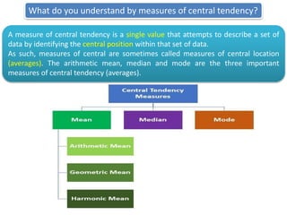
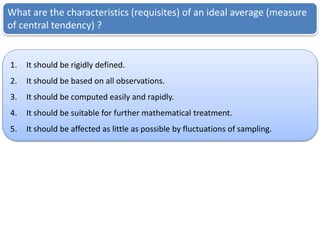
Title of the Course: Statistical Methods
Class: Second Year, First Semester
Teacher:
Dr. Ramkrishna Singh Solanki
Assistant Professor: Mathematics and Statistics
Contact: +919826026464
email: rsolankisolanki_stat@jnkvv.org
College of Agriculture Balaghat
Murjhad Farm, Waraseoni, M.P. 481331
“Measures of Central Tendency”
What do you understand by measures of central tendency?
A measure of central tendency is a single value that attempts to describe a set of
data by identifying the central position within that set of data.
As such, measures of central are sometimes called measures of central location
(averages). The arithmetic mean, median and mode are the three important
measures of central tendency (averages).
What are the characteristics (requisites) of an ideal average (measure
of central tendency) ?
1. It should be rigidly defined.
2. It should be based on all observations.
3. It should be computed easily and rapidly.
4. It should be suitable for further mathematical treatment.
5. It should be affected as little as possible by fluctuations of sampling.
The mean is the average of a data set.
The median is the middle of the set of numbers.
The mode is the most frequent number in a data set.
“Measures of Central Tendency”
Mean
Mean
Harmonic
Mean
Geometric
Mean
Arithmetic
Mean
Arithmetic Mean
Arithmetic mean (A.M.) of a set of observations is their sum divided by the number
of observations
1.Ungrouped data: The A.M. (x, sample) ( ,
population) of ‘n’ observations n
x
x
x ...,
,
, 2
1
=
n
x
n
x
x
x
n
i
i
n





 1
2
1
...
2.Grouped data:
(i) Discrete frequency distribution
A.M. =











n
i
i
n
i
i
i
n
n
n
f
x
f
f
f
f
x
f
x
f
x
f
1
1
2
1
2
2
1
1
...
...
(ii) Continuous frequency distribution: ‘x’ is taken as
the mid-value of the corresponding class.
55, 44, 87, 92, 15, 43, 98, 21,
class: 10-20 20-30 30-40 40-50
f: 2 5 4 7
X: 55 44 87 92 15 43 98 21
f: 2 5 4 7 4 1 2 3
Ungrouped
Grouped: Discrete frequency distribution
Grouped: Continues frequency distribution
Merits & Demerits of A.M.
Demerits:
1. It can neither be determined by inspection or by graphical location.
2. It can not be computed for qualitative data.
3. If any one of the data is missing then it can not be calculated.
Merits:
1. Arithmetic mean rigidly defined.
2. It is easy to calculate and simple to understand.
3. It is based on all observations .
4. It is suitable for further mathematical treatment.
5. It is least affected by the fluctuation of sampling.
Geometric Mean
Geometric mean (GM) is defined as the nth root of the product of n numbers
The G.M. of ‘n’ observations n
x
x
x ...,
,
, 2
1
= n
n
n
n x
x
x
x
x
x 





 ...
)
...
( 2
1
/
1
2
1
It is useful in averaging rates, ratios and percentages.
Geometric mean is considered as the best average in the construction of index numbers.
It is used to find the average percentage increase in sales, production, or other economic
or business series.
It is also used in relative change, as in the case of biological studies like cell division and
bacterial growth rate etc.
For example, if the prices of a commodity increased by 5, 10, and 18 percent over a span of
three years then the average annual increase is not 11% as given by the arithmetic mean.
The annual average growth rate is instead equal to the geometric mean which is equal to
10.9%
In practice we take the logarithms of the values and then proceed as in the case of mean.
The antilog of the mean of log values will give us geometric mean. This method holds
good for frequency distribution also.
Merits & Demerits of G.M.
Demerits:
1. If one of the observations is negative, the geometric mean will be imaginary.
2. It requires different mathematical knowledge ( logarithm, ratio, roots) to
determine geometric mean. So, it is complex to compute and difficult to
understand.
3. In case of open-ended frequency distribution, geometric mean cannot be
obtained.
Merits:
1. It is rigidly defined.
2. It is based on all observations .
3. It is suitable for further mathematical treatment.
4. It gives more weights to the small values and less weights to the large values.
5. It is used in averaging the ratios, percentages and in determining the rate
gradual increase and decrease.
we want to compare online ratings for two coffee shops using two different sources. The
problem is that source 1 uses a 5-star scale & source 2 uses a 100-point scale:
Coffee shop A: source 1 rating: 4.5 and source 2 rating: 68
Coffee shop B: source 1 rating: 3 and source 2 rating: 75
If we take the arithmetic mean of raw ratings for each coffee shop:
Coffee shop A = (4.5 + 68) ÷ 2 = 36.25 and Coffee shop B = (3 + 75) ÷ 2 = 39
We’d conclude that Coffee shop B was the winner.
We’d know that we have to normalize our values onto the same scale before averaging them
with the arithmetic mean, to get an accurate result. So we multiply the source 1 ratings by 20
to bring them from a 5-star scale to the 100-point scale of source 2:
Coffee shop A: 4.5 * 20 = 90 and (90 + 68) ÷ 2 = 79
Coffee shop B: 3 * 20 = 60 and (60 + 75) ÷ 2 = 67.5
So we find that Coffee shop A is the true winner.
The geometric mean, however, allows us to reach the same conclusion.
Coffee shop A = square root of (4.5 * 68) = 17.5
Coffee shop B = square root of (3 * 75) = 15
Harmonic Mean
The harmonic mean (HM) is the reciprocal of the arithmetic mean of the reciprocals.
The H.M. of ‘n’ observations n
x
x
x ...,
,
, 2
1
=
 











i
n x
n
x
x
x
n
1
1
.
.
.
1
1
2
1
Example: What is the harmonic mean of 2, 4 and 5?
Solution: The reciprocals of 2, 4 and 5 are:
= 0.5, = 0.25, = 0.2
Now adding the three results obtained: 0.5 + 0.25 + 0.2 = 0.95
Next, divide the result of the above step by the number of elements:
2
1
4
1
5
1
.
16
.
3
95
.
0
3
.
.
the
of
reciprocal
The
3
95
.
0





M
H
is
Mean
Arithmetic
Mean
Arithmetic
When to use?
Harmonic mean is helpful when dealing with data sets of rates or ratios (i.e.
fractions) over different lengths or periods. It is used to calculate the average value
when the values are expressed as value/unit. Since the speed is expressed as
km/hour, harmonic mean is used for the calculation of average speed. In finance, the
harmonic mean is used to calculate average multiples such as the price-earnings
ratio. It is also utilised by market technicians to discover patterns such as Fibonacci
Sequences.
Merits & Demerits of H.M.
Demerits:
1. All the values must be available for computation.
2. It is difficult to understand and compute.
3. Its value cannot be obtained if any one of the observations is zero.
Merits:
1. It is rigidly defined.
2. It is based on all observations .
3. It is suitable for further mathematical treatment.
4. It gives less weight to large items and more to small items.
5. The harmonic mean is especially useful in averaging rates and ratios where the
time factor is variable and the act being performed (e.g., distance) is constant.
“Measures of Central Tendency”
Median
22
Median
Median is the middle value of the distribution i.e median of a distribution is the
value of the variable which divides it into two equal parts when the items are
arranged in ascending or descending order.
It is the value of the variable such that the number of observations above it is equal
to the number of observations below it.
Definition
23
MERITS & DEMERITS OF MEDIAN
24
Merits:
1) It is easy to compute and understand.
2) It is well defined an ideal average should be.
3) It is not affected by extreme values.
4) It can be determined graphically.
5) It is proper average for qualitative data.
The median is less sensitive to outliers than the mean
MERITS & DEMERITS OF MEDIAN
26
Demerits:
1) For computing median data needs to be arranged in ascending
or descending order.
2) It is not based on all the observations of the data.
3) It can not be given further algebraic treatment.
4) It is affected by fluctuation of sampling.
5) In some cases median is determined approximately as the mid-
point of two observations.
APPLICATIONS OF MEDIAN
27
Applications:
1) When extreme values are not given then it is used to measure the
location.(for skewed distribution).
2) When measurement scale is ordinal that time median can be used.
3) For skewed data, median is used.
4) In some cases median gives us the accurate value than mean. For example,
if we are considering the salary of people, if one's salary is more than its
mean then so in such cases median is used.
5) Median is used to find middle most data. It is used to determine a point
from where 50% of data is more & 50% data is less. It is used where
extreme cases can be ignored. E.g. To find the performance of a cricketer
where his worst & best extreme performance can be ignored to give his
consistent performance.
MEDIAN FOR RAW DATA: Ungrouped data
In case of raw data (when data arranged in order) ,there are two cases
0 1 2 3 4 5 6 7 8 9 10
45 48 60 65 65 100
28
If n is odd, the median is the middle number i.e. (n+1)/2th term, where n is the
total number of observations.
If n is even, the median is the average of the two middle numbers i.e. (n/2)th and
((n+1)/2)th term.
Calculate the median for the data 24, 41, 30, 18, 22, 45, 36, 33 and 18
Solution: Firstly arrange the data in ascending order
Example for finding Median for raw data: Ungrouped data
Calculate the median for the data 17, 12, 18, 19, 15, 18, 12, 10, 18 and 15
Solution: Firstly arrange the data in ascending order
10, 12, 12, 15, 15, 17, 18, 18, 18, 19
Example for finding Median for raw data: Ungrouped data
MEDIAN FOR GROUPED DATA
1) Find N/2, where N is total number of observations i.e.
2) See the (less than) cumulative frequency just greater than N/2
3) The corresponding value of x is median
For Discrete Frequency Distribution, median is obtained by considering the cumulative
frequencies. The steps for calculating the median are given below:



n
i
i
f
N
1
31
32
MEDIAN FOR GROUPED DATA: Discrete Frequency Distribution
Example : Find the median of the following data:
x Frequency ( f )
1 8
2 10
3 11
4 16
5 20
6 25
7 15
8 9
9 6
Total
Solution
Calculate
the c.f.
x Frequency ( f ) c.f.
1 8 8
2 10 8 + 10 = 18
3 11 18 + 11 = 29
4 16 29 + 16 = 45
5 20 45 + 20 = 65
6 25 65 + 25 = 90
7 15 90 + 15 = 105
8 9 105 + 9 = 114
9 6 114 + 6 = 120
Total 120

  f
N
120

  f
N
60
2
120 


N
N
Here
The cumulative frequency just greater than N/2
is 65 and the value of x corresponding to 65 is 5.
Therefore Median = 5.
MEDIAN FOR GROUPED DATA: Continuous Frequency Distribution










 C
N
f
i
L
Median
2
1
Where
L1 = lower limit of median class
N = total number of observations i.e. sum of frequencies
C = cumulative frequency of the class previous the median class
f = frequency of median class
i = class width i.e. Magnitude of median class
For Continuous Frequency Distribution, median is given by the formula:
33
Median class: The class which contains ( N/2 )th term.
34
Class Frequency ( f )
1-5 2
5-10 4
10-15 9
15-20 7
20-25 5
25-30 3
Total 30

  f
N
Example : Find the median of the following data:
Class Frequency ( f ) c.f.
1-5 2 2
5-10 4 2+4 = 6
10-15 9 6 + 9 = 15
15-20 7 15 + 7 = 22
20-25 5 22 + 5 = 27
25-30 3 27 + 3 = 30
Total 30

  f
N
Solution
Calculate
the c.f.
Median number = ( N / 2 ) = 15
Median class = 10 – 15
Now
L1 = 10, i = 5, f = 9, N = 30, C = 6
04
.
15
6
2
30
9
5
10
2
1






















 C
N
f
i
L
Median
MEDIAN FOR GROUPED DATA: Continuous Frequency Distribution
“Measures of Central Tendency”
Mode
Mode
The mode is the value that appears most frequently in a data set.
Definition
The mode is the value that occurs most often.
MERITS & DEMERITS OF MODE
Merits:
1) The mode is easy to understand and calculate.
2) The mode is not affected by extreme values.
3) The mode is easy to identify in a data set and in a discrete frequency distribution.
4) The mode is useful for qualitative data.
5) The mode can be computed in an open-ended frequency table.
6) The mode can be located graphically.
Demerits:
1) The mode is not defined when there are no repeats in a data set.
2) The mode is not based on all values.
3) The mode is unstable when the data consist of a small number of values.
4) Sometimes data have one mode, more than one mode, or no mode at all.
APPLICATIONS OF MODE
1. Mode is most useful as a measure of central tendency when examining
categorical data, such as models of cars or flavors of soda, for which a
mathematical average median value based on ordering can not be calculated.
2. Mode is used where we need to find the most frequent data. e.g. if we need to
find the most favorite Subject of students in a given class, mode can be used.
3. To find the most common size of the shoes sold in a shop.
4. A clothing store might use the mode to determine the most popular size of jeans
to stock.
5. A marketing company might use the mode to determine the most popular color
of car among its target audience.
MODE FOR RAW DATA: Ungrouped data
In case of raw data, we guess mode by inspection. We observe that term in the data
which occurs maximum number of times. This term is called mode.
Example: Find the mode for following series
3, 3, 6, 9, 16, 16, 16, 27, 27, 37, 48
Solution:
In the following series of numbers, 16 is the mode since it appears more
times (i.e. frequency is maximum) in the set than any other number:
3, 3, 6, 9, 16, 16, 16, 27, 27, 37, 48
Thus,
Mode = 16
MODE FOR GROUPED DATA: Discrete Frequency Distribution
For Discrete Frequency Distribution, mode is the value of the variable corresponding
to maximum frequency.
Example: Calculate mode from the following data:
No. of days
with rain (X )
No. of weeks
( f )
0 2
1 5
2 5
3 4
4 14
5 9
6 7
7 1
Solution: Since the frequency corresponding to
the value 4 is maximum hence Mode = 4.
Maximum frequency
MODE FOR GROUPED DATA: Continuous frequency distribution
 
 
i
f
f
f
f
f
L
Mode 





2
0
1
0
1
1
2
In the case of Continuous Frequency Distribution mode is given by the formula:
Where,
L1 = lower limit of the modal class
f1 = frequency of the modal class
f0 = frequency of the class previous the modal class
f2 = frequency of the class next the modal class
i = width of the modal class
Modal class: the class interval within a set of data that contains the most number
of data points, which we can view as the highest frequency.
Example: In a class of 30 students marks obtained by students in mathematics out of 50
is tabulated as below. Calculate the mode of data given.
Class Interval Frequency (f)
10 – 20 5
20 – 30 12
30 – 40 8
40 – 50 5
Total = 30
Solution
Find the
Modal
class
Class Interval Frequency (f)
10 – 20 5 f0
20 – 30 12 f1
30 – 40 8 f2
40 – 50 5
Total N = 30
The maximum frequency is 12 and the class interval corresponding to this
frequency is 20 – 30. Thus, the modal class is 20 – 30.
Hence,
L1 = 20
f1 = 12
f0 = 5
f2 = 8
i = (30 - 20) = 10
 
 
i
f
f
f
f
f
L
Mode 





2
0
1
0
1
1
2
 
 
.
36
.
20
10
8
5
12
2
5
12
20








Mode
Unimodal: Only one values that occurs with the maximum frequency.
Bimodal: Only two values occurs with the same maximum frequency.
Multimodal: More than two values with the same maximum frequency.
No mode: No value is repeated more than once.
Statistical Methods: Measures of Central Tendency.pptx

Statistical Methods: Measures of Central Tendency.pptx

  • 1.
    Title of theCourse: Statistical Methods Class: Second Year, First Semester Teacher: Dr. Ramkrishna Singh Solanki Assistant Professor: Mathematics and Statistics Contact: +919826026464 email: rsolankisolanki_stat@jnkvv.org College of Agriculture Balaghat Murjhad Farm, Waraseoni, M.P. 481331
  • 2.
  • 3.
    What do youunderstand by measures of central tendency? A measure of central tendency is a single value that attempts to describe a set of data by identifying the central position within that set of data. As such, measures of central are sometimes called measures of central location (averages). The arithmetic mean, median and mode are the three important measures of central tendency (averages).
  • 4.
    What are thecharacteristics (requisites) of an ideal average (measure of central tendency) ? 1. It should be rigidly defined. 2. It should be based on all observations. 3. It should be computed easily and rapidly. 4. It should be suitable for further mathematical treatment. 5. It should be affected as little as possible by fluctuations of sampling.
  • 5.
    The mean isthe average of a data set. The median is the middle of the set of numbers. The mode is the most frequent number in a data set.
  • 6.
    “Measures of CentralTendency” Mean
  • 7.
  • 8.
    Arithmetic Mean Arithmetic mean(A.M.) of a set of observations is their sum divided by the number of observations 1.Ungrouped data: The A.M. (x, sample) ( , population) of ‘n’ observations n x x x ..., , , 2 1 = n x n x x x n i i n       1 2 1 ... 2.Grouped data: (i) Discrete frequency distribution A.M. =            n i i n i i i n n n f x f f f f x f x f x f 1 1 2 1 2 2 1 1 ... ... (ii) Continuous frequency distribution: ‘x’ is taken as the mid-value of the corresponding class. 55, 44, 87, 92, 15, 43, 98, 21, class: 10-20 20-30 30-40 40-50 f: 2 5 4 7 X: 55 44 87 92 15 43 98 21 f: 2 5 4 7 4 1 2 3
  • 9.
  • 10.
  • 11.
  • 12.
    Merits & Demeritsof A.M. Demerits: 1. It can neither be determined by inspection or by graphical location. 2. It can not be computed for qualitative data. 3. If any one of the data is missing then it can not be calculated. Merits: 1. Arithmetic mean rigidly defined. 2. It is easy to calculate and simple to understand. 3. It is based on all observations . 4. It is suitable for further mathematical treatment. 5. It is least affected by the fluctuation of sampling.
  • 13.
    Geometric Mean Geometric mean(GM) is defined as the nth root of the product of n numbers The G.M. of ‘n’ observations n x x x ..., , , 2 1 = n n n n x x x x x x        ... ) ... ( 2 1 / 1 2 1 It is useful in averaging rates, ratios and percentages. Geometric mean is considered as the best average in the construction of index numbers. It is used to find the average percentage increase in sales, production, or other economic or business series. It is also used in relative change, as in the case of biological studies like cell division and bacterial growth rate etc. For example, if the prices of a commodity increased by 5, 10, and 18 percent over a span of three years then the average annual increase is not 11% as given by the arithmetic mean. The annual average growth rate is instead equal to the geometric mean which is equal to 10.9%
  • 15.
    In practice wetake the logarithms of the values and then proceed as in the case of mean. The antilog of the mean of log values will give us geometric mean. This method holds good for frequency distribution also.
  • 16.
    Merits & Demeritsof G.M. Demerits: 1. If one of the observations is negative, the geometric mean will be imaginary. 2. It requires different mathematical knowledge ( logarithm, ratio, roots) to determine geometric mean. So, it is complex to compute and difficult to understand. 3. In case of open-ended frequency distribution, geometric mean cannot be obtained. Merits: 1. It is rigidly defined. 2. It is based on all observations . 3. It is suitable for further mathematical treatment. 4. It gives more weights to the small values and less weights to the large values. 5. It is used in averaging the ratios, percentages and in determining the rate gradual increase and decrease.
  • 17.
    we want tocompare online ratings for two coffee shops using two different sources. The problem is that source 1 uses a 5-star scale & source 2 uses a 100-point scale: Coffee shop A: source 1 rating: 4.5 and source 2 rating: 68 Coffee shop B: source 1 rating: 3 and source 2 rating: 75 If we take the arithmetic mean of raw ratings for each coffee shop: Coffee shop A = (4.5 + 68) ÷ 2 = 36.25 and Coffee shop B = (3 + 75) ÷ 2 = 39 We’d conclude that Coffee shop B was the winner. We’d know that we have to normalize our values onto the same scale before averaging them with the arithmetic mean, to get an accurate result. So we multiply the source 1 ratings by 20 to bring them from a 5-star scale to the 100-point scale of source 2: Coffee shop A: 4.5 * 20 = 90 and (90 + 68) ÷ 2 = 79 Coffee shop B: 3 * 20 = 60 and (60 + 75) ÷ 2 = 67.5 So we find that Coffee shop A is the true winner. The geometric mean, however, allows us to reach the same conclusion. Coffee shop A = square root of (4.5 * 68) = 17.5 Coffee shop B = square root of (3 * 75) = 15
  • 18.
    Harmonic Mean The harmonicmean (HM) is the reciprocal of the arithmetic mean of the reciprocals. The H.M. of ‘n’ observations n x x x ..., , , 2 1 =              i n x n x x x n 1 1 . . . 1 1 2 1
  • 19.
    Example: What isthe harmonic mean of 2, 4 and 5? Solution: The reciprocals of 2, 4 and 5 are: = 0.5, = 0.25, = 0.2 Now adding the three results obtained: 0.5 + 0.25 + 0.2 = 0.95 Next, divide the result of the above step by the number of elements: 2 1 4 1 5 1 . 16 . 3 95 . 0 3 . . the of reciprocal The 3 95 . 0      M H is Mean Arithmetic Mean Arithmetic When to use? Harmonic mean is helpful when dealing with data sets of rates or ratios (i.e. fractions) over different lengths or periods. It is used to calculate the average value when the values are expressed as value/unit. Since the speed is expressed as km/hour, harmonic mean is used for the calculation of average speed. In finance, the harmonic mean is used to calculate average multiples such as the price-earnings ratio. It is also utilised by market technicians to discover patterns such as Fibonacci Sequences.
  • 20.
    Merits & Demeritsof H.M. Demerits: 1. All the values must be available for computation. 2. It is difficult to understand and compute. 3. Its value cannot be obtained if any one of the observations is zero. Merits: 1. It is rigidly defined. 2. It is based on all observations . 3. It is suitable for further mathematical treatment. 4. It gives less weight to large items and more to small items. 5. The harmonic mean is especially useful in averaging rates and ratios where the time factor is variable and the act being performed (e.g., distance) is constant.
  • 22.
    “Measures of CentralTendency” Median 22
  • 23.
    Median Median is themiddle value of the distribution i.e median of a distribution is the value of the variable which divides it into two equal parts when the items are arranged in ascending or descending order. It is the value of the variable such that the number of observations above it is equal to the number of observations below it. Definition 23
  • 24.
    MERITS & DEMERITSOF MEDIAN 24 Merits: 1) It is easy to compute and understand. 2) It is well defined an ideal average should be. 3) It is not affected by extreme values. 4) It can be determined graphically. 5) It is proper average for qualitative data.
  • 25.
    The median isless sensitive to outliers than the mean
  • 26.
    MERITS & DEMERITSOF MEDIAN 26 Demerits: 1) For computing median data needs to be arranged in ascending or descending order. 2) It is not based on all the observations of the data. 3) It can not be given further algebraic treatment. 4) It is affected by fluctuation of sampling. 5) In some cases median is determined approximately as the mid- point of two observations.
  • 27.
    APPLICATIONS OF MEDIAN 27 Applications: 1)When extreme values are not given then it is used to measure the location.(for skewed distribution). 2) When measurement scale is ordinal that time median can be used. 3) For skewed data, median is used. 4) In some cases median gives us the accurate value than mean. For example, if we are considering the salary of people, if one's salary is more than its mean then so in such cases median is used. 5) Median is used to find middle most data. It is used to determine a point from where 50% of data is more & 50% data is less. It is used where extreme cases can be ignored. E.g. To find the performance of a cricketer where his worst & best extreme performance can be ignored to give his consistent performance.
  • 28.
    MEDIAN FOR RAWDATA: Ungrouped data In case of raw data (when data arranged in order) ,there are two cases 0 1 2 3 4 5 6 7 8 9 10 45 48 60 65 65 100 28 If n is odd, the median is the middle number i.e. (n+1)/2th term, where n is the total number of observations. If n is even, the median is the average of the two middle numbers i.e. (n/2)th and ((n+1)/2)th term.
  • 29.
    Calculate the medianfor the data 24, 41, 30, 18, 22, 45, 36, 33 and 18 Solution: Firstly arrange the data in ascending order Example for finding Median for raw data: Ungrouped data
  • 30.
    Calculate the medianfor the data 17, 12, 18, 19, 15, 18, 12, 10, 18 and 15 Solution: Firstly arrange the data in ascending order 10, 12, 12, 15, 15, 17, 18, 18, 18, 19 Example for finding Median for raw data: Ungrouped data
  • 31.
    MEDIAN FOR GROUPEDDATA 1) Find N/2, where N is total number of observations i.e. 2) See the (less than) cumulative frequency just greater than N/2 3) The corresponding value of x is median For Discrete Frequency Distribution, median is obtained by considering the cumulative frequencies. The steps for calculating the median are given below:    n i i f N 1 31
  • 32.
    32 MEDIAN FOR GROUPEDDATA: Discrete Frequency Distribution Example : Find the median of the following data: x Frequency ( f ) 1 8 2 10 3 11 4 16 5 20 6 25 7 15 8 9 9 6 Total Solution Calculate the c.f. x Frequency ( f ) c.f. 1 8 8 2 10 8 + 10 = 18 3 11 18 + 11 = 29 4 16 29 + 16 = 45 5 20 45 + 20 = 65 6 25 65 + 25 = 90 7 15 90 + 15 = 105 8 9 105 + 9 = 114 9 6 114 + 6 = 120 Total 120    f N 120    f N 60 2 120    N N Here The cumulative frequency just greater than N/2 is 65 and the value of x corresponding to 65 is 5. Therefore Median = 5.
  • 33.
    MEDIAN FOR GROUPEDDATA: Continuous Frequency Distribution            C N f i L Median 2 1 Where L1 = lower limit of median class N = total number of observations i.e. sum of frequencies C = cumulative frequency of the class previous the median class f = frequency of median class i = class width i.e. Magnitude of median class For Continuous Frequency Distribution, median is given by the formula: 33 Median class: The class which contains ( N/2 )th term.
  • 34.
    34 Class Frequency (f ) 1-5 2 5-10 4 10-15 9 15-20 7 20-25 5 25-30 3 Total 30    f N Example : Find the median of the following data: Class Frequency ( f ) c.f. 1-5 2 2 5-10 4 2+4 = 6 10-15 9 6 + 9 = 15 15-20 7 15 + 7 = 22 20-25 5 22 + 5 = 27 25-30 3 27 + 3 = 30 Total 30    f N Solution Calculate the c.f. Median number = ( N / 2 ) = 15 Median class = 10 – 15 Now L1 = 10, i = 5, f = 9, N = 30, C = 6 04 . 15 6 2 30 9 5 10 2 1                        C N f i L Median MEDIAN FOR GROUPED DATA: Continuous Frequency Distribution
  • 35.
    “Measures of CentralTendency” Mode
  • 36.
    Mode The mode isthe value that appears most frequently in a data set. Definition The mode is the value that occurs most often.
  • 37.
    MERITS & DEMERITSOF MODE Merits: 1) The mode is easy to understand and calculate. 2) The mode is not affected by extreme values. 3) The mode is easy to identify in a data set and in a discrete frequency distribution. 4) The mode is useful for qualitative data. 5) The mode can be computed in an open-ended frequency table. 6) The mode can be located graphically. Demerits: 1) The mode is not defined when there are no repeats in a data set. 2) The mode is not based on all values. 3) The mode is unstable when the data consist of a small number of values. 4) Sometimes data have one mode, more than one mode, or no mode at all.
  • 38.
    APPLICATIONS OF MODE 1.Mode is most useful as a measure of central tendency when examining categorical data, such as models of cars or flavors of soda, for which a mathematical average median value based on ordering can not be calculated. 2. Mode is used where we need to find the most frequent data. e.g. if we need to find the most favorite Subject of students in a given class, mode can be used. 3. To find the most common size of the shoes sold in a shop. 4. A clothing store might use the mode to determine the most popular size of jeans to stock. 5. A marketing company might use the mode to determine the most popular color of car among its target audience.
  • 39.
    MODE FOR RAWDATA: Ungrouped data In case of raw data, we guess mode by inspection. We observe that term in the data which occurs maximum number of times. This term is called mode. Example: Find the mode for following series 3, 3, 6, 9, 16, 16, 16, 27, 27, 37, 48 Solution: In the following series of numbers, 16 is the mode since it appears more times (i.e. frequency is maximum) in the set than any other number: 3, 3, 6, 9, 16, 16, 16, 27, 27, 37, 48 Thus, Mode = 16
  • 40.
    MODE FOR GROUPEDDATA: Discrete Frequency Distribution For Discrete Frequency Distribution, mode is the value of the variable corresponding to maximum frequency. Example: Calculate mode from the following data: No. of days with rain (X ) No. of weeks ( f ) 0 2 1 5 2 5 3 4 4 14 5 9 6 7 7 1 Solution: Since the frequency corresponding to the value 4 is maximum hence Mode = 4. Maximum frequency
  • 41.
    MODE FOR GROUPEDDATA: Continuous frequency distribution     i f f f f f L Mode       2 0 1 0 1 1 2 In the case of Continuous Frequency Distribution mode is given by the formula: Where, L1 = lower limit of the modal class f1 = frequency of the modal class f0 = frequency of the class previous the modal class f2 = frequency of the class next the modal class i = width of the modal class Modal class: the class interval within a set of data that contains the most number of data points, which we can view as the highest frequency.
  • 42.
    Example: In aclass of 30 students marks obtained by students in mathematics out of 50 is tabulated as below. Calculate the mode of data given. Class Interval Frequency (f) 10 – 20 5 20 – 30 12 30 – 40 8 40 – 50 5 Total = 30 Solution Find the Modal class Class Interval Frequency (f) 10 – 20 5 f0 20 – 30 12 f1 30 – 40 8 f2 40 – 50 5 Total N = 30 The maximum frequency is 12 and the class interval corresponding to this frequency is 20 – 30. Thus, the modal class is 20 – 30. Hence, L1 = 20 f1 = 12 f0 = 5 f2 = 8 i = (30 - 20) = 10     i f f f f f L Mode       2 0 1 0 1 1 2     . 36 . 20 10 8 5 12 2 5 12 20         Mode
  • 43.
    Unimodal: Only onevalues that occurs with the maximum frequency. Bimodal: Only two values occurs with the same maximum frequency. Multimodal: More than two values with the same maximum frequency. No mode: No value is repeated more than once.