Exploring different analysis for the given speed data of different categories of vehicles using SPSS Software MADE BY- SHRIKRISHNA KESHARWANI

1. A Report On –
EXPERIMENT - 7
(Statistical Data Analysis Using SPSS Software)
Submitted by-
SHRIKRISHNA KESHARWANI
Roll no.-
22CEM3R23
Subject-
TRANSPORTATION ANALYTICS LABORATORY
Bachelor of Technology
In
TRANSPORTATION ENGINEERING
DEPARTMENT OF CIVIL ENGINEERING
NATIONAL INSTITUTE OF TECHNOLOGY WARANGAL
OCTOBER, 2022

2. Transportation Analytics Laboratory
SHRIKRISHNA KESHARWANI (22CEM3R23) 2
Table of Contents
1. Objectives-..........................................................................................................................3
2. Software Used- ...................................................................................................................3
3. Theory- ...............................................................................................................................3
3.1 Descriptive Statistics........................................................................................................3
3.2 Inferential Statistics .........................................................................................................5
4. Procedure-...........................................................................................................................5
5.1 Descriptive Statistics- ......................................................................................................6
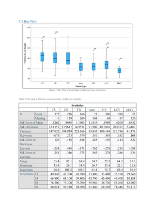
5.2 Box Plot-..........................................................................................................................7
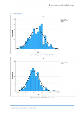
5.3 Histograms-......................................................................................................................8
5.4 Cumulative Frequency Curves:......................................................................................11
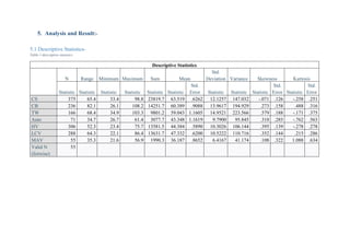
6. Results & Discussion:.......................................................................................................15
7. Conclusion........................................................................................................................15
References................................................................................................................................15
List of Tables-
Table 1 descriptive statistics......................................................................................................6
Table 2 Descriptive Statistics and percentiles of different variables.........................................7
List of Figures-
Figure 1 Box Plot of speed data of different types of vehicles..................................................7
Figure 2 Histogram of speed data for Small Car .......................................................................8
Figure 3 Histogram of speed data for Big Car...........................................................................8
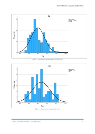
Figure 4 Histogram of speed data for Two Wheelers................................................................9
Figure 5 Histogram of speed data for Auto ...............................................................................9
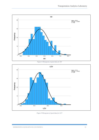
Figure 6 Histogram of speed data for HV................................................................................10
Figure 7 Histogram of speed data for LCV .............................................................................10
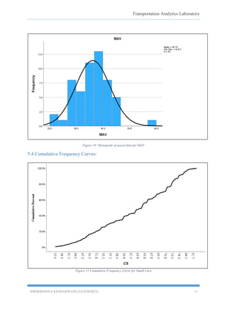
Figure 8 Histogram of speed data for MAV ...........................................................................11
Figure 9 Cumulative Frequency Curve for Small Cars ...........................................................11
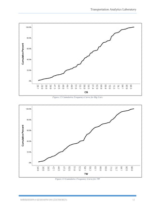
Figure 10 Cumulative Frequency Curve for Big Cars.............................................................12
Figure 11 Cumulative Frequency Curve for TW.....................................................................12
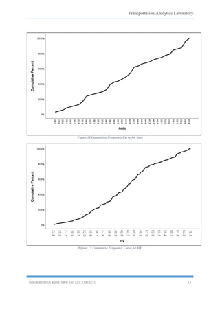
Figure 12 Cumulative Frequency Curve for Auto ...................................................................13
Figure 13 Cumulative Frequency Curve for HV .....................................................................13
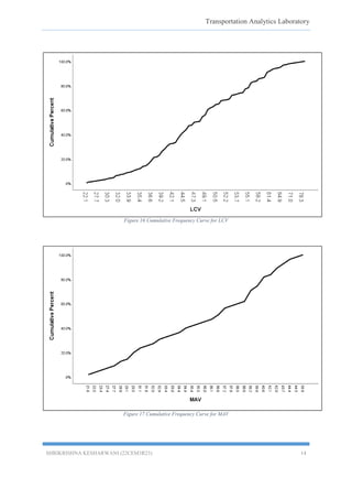
Figure 14 Cumulative Frequency Curve for LCV ...................................................................14
Figure 15 Cumulative Frequency Curve for MAV..................................................................14

3. Transportation Analytics Laboratory
SHRIKRISHNA KESHARWANI (22CEM3R23) 3
1. Objectives-
Exploring different analysis for the given speed data of different categories of vehicles using
SPSS Software.
2. Software Used-
IBM SPSS statistics.
3. Theory-
Transportation engineering deals with a lot of data involved with a wide range of parameters.
To get a better idea regarding how the data is indicated the analysis of data is an important
phase. Some of the analysis that are very basic in dealing with this data are creating basic box
plots, histograms, and frequency curves.
3.1 Descriptive Statistics
a) Mean: The mean of a series of data is the value equal to the sum of the values of
all the observations divided by the number of observations.
b) Median: In statistics and probability theory, a median is a value separating the
higher half from the lower half of a data sample, a population or a probability
distribution.
c) Range: The Range is the difference between the lowest and highest values.
d) Standard Deviation: In statistics, the standard deviation is a measure of the amount
of variation or dispersion of a set of values. A low standard deviation indicates that
the values tend to be close to the mean of the set, while a high standard deviation
indicates that the values are spread out over a wider range.
e) Variance: In statistics, variance is the expectation of the squared deviation of a
random variable from its mean. Informally, it measures how far a set of numbers is
spread out from their average value.
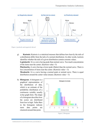
f) Skewness: Skewness is a measure of the degree of asymmetry of a frequency
distribution. In general, when the distribution stretches to the right more than it does
to the left, it can be said that the distribution is right-skewed, or positively skewed.
When a distribution is right skewed, the mean is to the right of the median, which
in turn is to the right of the mode. The opposite is true for left-skewed distribution.

4. Transportation Analytics Laboratory
SHRIKRISHNA KESHARWANI (22CEM3R23) 4
Figure 1 positively and negatively skewed
g) Kurtosis: Kurtosis is a statistical measure that defines how heavily the tails of
a distribution differ from the tails of a normal distribution. In other words, kurtosis
identifies whether the tails of a given distribution contain extreme values.
Leptokurtic: It is a curve having peak than normal curve. Too much concentration
of the items near the center. (Kurtosis value >3)
Platykurtic: A curve having a lower peak (flatter) than the normal curve. There is
less concentration of items near the center. (Kurtosis value < 3)
Mesokurtic: It is a curve having a normal peak or normal curve. There is equal
distribution around the center value (mean). (Kurtosis value = 3)
h) Histogram: A histogram is a
graphical representation of
the distribution of data,
which is an estimate of the
probability distribution of a
continuous variable, usually
in bar graph form. The shape
of a histogram describes how
the scores are distributed
from low to high. Taller Bars
in the histogram indicate
more data points are
clustered around that point.
Figure 2 Histogram

5. Transportation Analytics Laboratory
SHRIKRISHNA KESHARWANI (22CEM3R23) 5
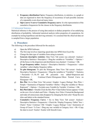
i) Frequency distribution Curve: Frequency distribution, in statistics, is a graph or
data set organized to show the frequency of occurrence of each possible outcome
of a repeatable event observed many times.
j) Ogive curve/ S curve/ Cumulative frequency curve: It is the representation of the
cumulative frequencies for the classes in the frequency distribution.
3.2 Inferential Statistics
Statistical inference is the process of using data analysis to deduce properties of an underlying
distribution of probability. Inferential statistical analysis infers properties of a population, for
example by testing hypotheses and deriving estimates. It is assumed that the observed data set
is sampled from a larger population.
4. Procedure-
The following is the procedure followed for the analysis:
a) Open the SPSS Software.
b) The first step involves importing speed data into SPSS from Excel file.
c) Change the data type of variables from string to numeric.
d) Generate descriptive statistics: Data View Tab screen was selected> Analyse>
Descriptive Statistics> Descriptive > Drag the variables to “Variables” > Options >
all the boxes in the dispersion and distribution was checked > Continue > OK
e) To get frequency tables: Analyse > Descriptive Statistics > Frequencies > select
variables> select display frequency tables.
f) To plot histogram: To plot the Histogram: Data View Tab screen> Analyse>
Descriptive Statistics> Frequencies > Drag the variables to “Variables” > Statistics
> Percentile> 15, 50, 85 and 98 percentile was added>Dispersion and
Distribution > Continue>Charts>Histograms>Show Normal Curve on
Histogram> OK.
g) Box Plot: Go to Data View Tab screen> Graphs> Legacy Dialogs> Box Plots >
Simple > Summaries of Separate Variables> Define > Drag the variables to “Boxes
Represent” > Options > Exclude cases Variable by Variable >Continue > OK.
h) Box Plot Editor: • Double Click the Box Plot • Chart Editor Screen appears • Click
on the axis • Go to Labels and Ticks > Display Axis Titles • Format the Background
and make all unnecessary data disappear by changing the font color • Keep the axis
titles and labels in the standard format.
i) Cumulative Frequency Curve: • Go to Data View Tab screen> Analyze>
Descriptive Statistics> Frequencies > Check the ‘Display Frequency Tables” box >
Charts> None> Continue> OK • Graphs> Legacy Dialogs> Line> Summaries of
Group of Cases> % Cum > Drag any one variable to Category Axis > Ok • Copy
the data to excel> Scatter> Scatter with Smooth Lines.

6. 5. Analysis and Result:-
5.1 Descriptive Statistics-
Table 1 descriptive statistics
Descriptive Statistics
N Range Minimum Maximum Sum Mean
Std.
Deviation Variance Skewness Kurtosis
Statistic Statistic Statistic Statistic Statistic Statistic
Std.
Error Statistic Statistic Statistic
Std.
Error Statistic
Std.
Error
CS 375 65.4 33.4 98.8 23819.7 63.519 .6262 12.1257 147.032 -.071 .126 -.258 .251
CB 236 82.1 26.1 108.2 14251.7 60.389 .9088 13.9617 194.929 .273 .158 .488 .316
TW 166 68.4 34.9 103.3 9801.2 59.043 1.1605 14.9521 223.566 .579 .188 -.171 .375
Auto 71 34.7 26.7 61.4 3077.7 43.348 1.1619 9.7900 95.845 .310 .285 -.762 .563
HV 306 52.3 23.4 75.7 13581.5 44.384 .5890 10.3026 106.144 .395 .139 -.278 .278
LCV 288 64.3 22.1 86.4 13631.7 47.332 .6200 10.5222 110.716 .352 .144 .215 .286
MAV 55 35.3 21.6 56.9 1990.3 36.187 .8652 6.4167 41.174 .108 .322 1.088 .634
Valid N
(listwise)
55

7. 5.2 Box Plot-
Figure 3 Box Plot of speed data of different types of vehicles
Table 2 Descriptive Statistics and percentiles of different variables
Statistics
CS CB TW Auto HV LCV MAV
N Valid 375 236 166 71 306 288 55
Missing 0 139 209 304 69 87 320
Std. Error of Mean .6262 .9088 1.1605 1.1619 .5890 .6200 .8652
Std. Deviation 12.1257 13.9617 14.9521 9.7900 10.3026 10.5222 6.4167
Variance 147.032 194.929 223.566 95.845 106.144 110.716 41.174
Skewness -.071 .273 .579 .310 .395 .352 .108
Std. Error of
Skewness
.126 .158 .188 .285 .139 .144 .322
Kurtosis -.258 .488 -.171 -.762 -.278 .215 1.088
Std. Error of
Kurtosis
.251 .316 .375 .563 .278 .286 .634
Range 65.4 82.1 68.4 34.7 52.3 64.3 35.3
Minimum 33.4 26.1 34.9 26.7 23.4 22.1 21.6
Maximum 98.8 108.2 103.3 61.4 75.7 86.4 56.9
Percentiles 15 49.840 47.300 43.700 33.400 33.400 36.100 29.260
58 66.800 63.100 59.800 43.700 45.400 49.400 38.188
85 76.300 73.300 75.700 55.960 56.730 58.200 42.900
98 88.024 93.220 94.700 61.400 68.520 71.440 55.412

8. Transportation Analytics Laboratory
SHRIKRISHNA KESHARWANI (22CEM3R23) 8
5.3 Histograms-
Figure 4 Histogram of speed data for Small Car
Figure 5 Histogram of speed data for Big Car

9. Transportation Analytics Laboratory
SHRIKRISHNA KESHARWANI (22CEM3R23) 9
Figure 6 Histogram of speed data for Two Wheelers
Figure 7 Histogram of speed data for Auto

10. Transportation Analytics Laboratory
SHRIKRISHNA KESHARWANI (22CEM3R23) 10
Figure 8 Histogram of speed data for HV
Figure 9 Histogram of speed data for LCV

11. Transportation Analytics Laboratory
SHRIKRISHNA KESHARWANI (22CEM3R23) 11
Figure 10 Histogram of speed data for MAV
5.4 Cumulative Frequency Curves:
Figure 11 Cumulative Frequency Curve for Small Cars

12. Transportation Analytics Laboratory
SHRIKRISHNA KESHARWANI (22CEM3R23) 12
Figure 12 Cumulative Frequency Curve for Big Cars
Figure 13 Cumulative Frequency Curve for TW

13. Transportation Analytics Laboratory
SHRIKRISHNA KESHARWANI (22CEM3R23) 13
Figure 14 Cumulative Frequency Curve for Auto
Figure 15 Cumulative Frequency Curve for HV

14. Transportation Analytics Laboratory
SHRIKRISHNA KESHARWANI (22CEM3R23) 14
Figure 16 Cumulative Frequency Curve for LCV
Figure 17 Cumulative Frequency Curve for MAV

15. Transportation Analytics Laboratory
SHRIKRISHNA KESHARWANI (22CEM3R23) 15
6. Results & Discussion:
Different analysis for the given speed data of different categories of vehicles using SPSS
Software.
7. Conclusion
This analysis done by the SPSS software can be compared with the other software by the
means of effectiveness, efficiency and data handling.
References
Agrawal, B. L. (n.d.). Basic Statistics . New age Publications.
Kadiyali, L. R. (2013). Traffic engineering and transport planning. Khanna publishers.