Statistical & Quality Control
Chapter_5
FUNDAMENTALS
OF STATISTICS
Definition of Statistics
The word statistics has two generally accepted
meanings:
1. A collection of quantitative data pertaining to
any subject or group, especially when the data are
systematically gathered and collated. Examples of
this meaning are blood pressure statistics, statistics
of a football game, employment statistics, and
accident statistics, to name a few.
Definition of Statistics
2. The science that deals with the collection,
tabulation, analysis, interpretation, and
presentation of quantitative data.
The use of statistics in quality deals with the second
and broader meaning and involves the divisions of
collecting, tabulating, analyzing, interpreting, and
presenting the quantitative data.
Definition of Statistics
There are two phases of statistics:
1. Descriptive or deductive statistics, which
endeavor to describe and analyze a subject or
group.
2. Inductive statistics, which endeavor to determine
from a limited amount of data (sample) an
important conclusion about a much larger amount
of data (population). Because these conclusions or
inferences cannot be stated with absolute certainty,
the language of probability is often used.
Definition of Statistics
Data may be collected by direct observation or
indirectly through written or verbal questions.
Data that are collected for quality purposes are
obtained by direct observation and are classified
as either variables or attributes.
Variables are those quality characteristics that
are measurable, such as a weight measured in
grams.
Collectingthe Data
Attributes, on the other hand, are those quality
characteristics that are classified as either
conforming or not conforming to specifications.
A variable that is capable of any degree of
subdivision is referred to as continuous. The
weight of a gray iron casting, which can be
measured as 11 kg, 11.33 kg, or 11.3398 kg (25
lb),
Collectingthe Data
Variables that exhibit gaps are called discrete. The
number of nonconforming rivets in a travel trailer
can be any whole number, such as 0, 3, 5, 10, 96,
however, there cannot be, say, 4.65 nonconforming
Sometimes it is convenient for verbal or
nonnumeric data to assume the nature of a
variable. For example, the quality of the surface
finish of a piece of furniture can be classified as
poor, average, or good.
Collectingthe Data
Collecting the Data
Measuring instruments may not give a true
reading because of problems due to accuracy
and precision
Collecting the Data
Based on this rounding rule, a rounded number
is an approximation of the exact number.
Thus, the rounded number 6.23 lies between
6.225 and 6.235 and is expressed as 6.225 ≤
6.23 6 < 6.235
The precision = 6.235 – 6.225 = 0.010
An associated term is greatest possible error
(g.p.e.),
which is one-half the precision or 0.010/2 =
0.005.
Collecting the Data
Sometimes precision and g.p.e. are not
adequate to describe error. For example,
the numbers 8765.4 and 3.2
have the same precision (0.10) and g.p.e.
(0.05); however, the relative error (r.e.) is
much different.
Describing the Data
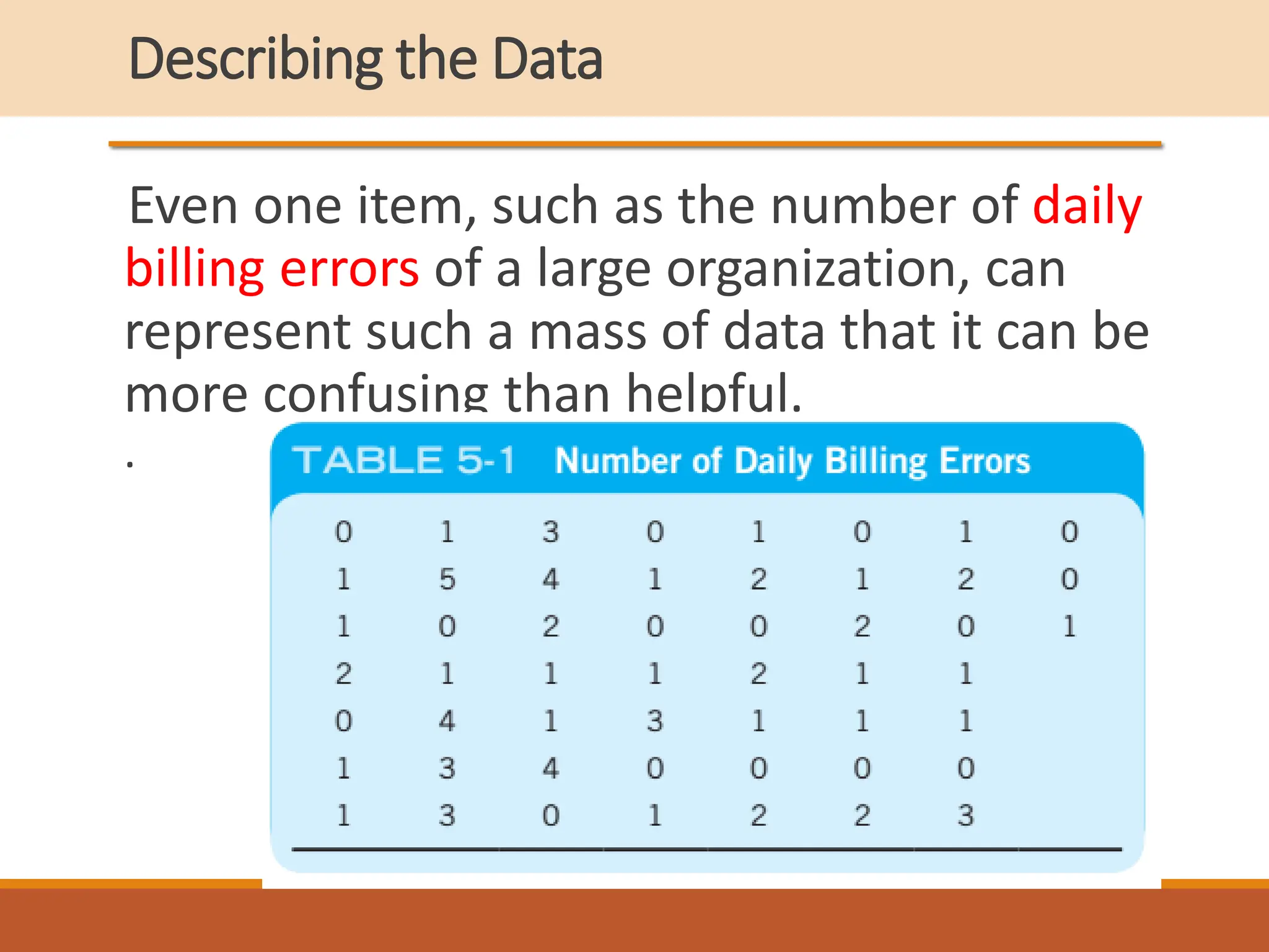
Even one item, such as the number of daily
billing errors of a large organization, can
represent such a mass of data that it can be
more confusing than helpful.
.
Describing the Data
Consider the data shown in Table 5-1 . Clearly these
data, in this form, are difficult to use and are not
effective in describing the data’s characteristics.
Some means of summarizing the data are needed
to show what value or values the data tend to
cluster about and how the data are dispersed or
spread out.
Two techniques are available to accomplish
this summarization of data—graphical and
analytical.
The graphical technique is a plot or picture
of a frequency distribution, which is a
summarization of how the data points
(observations) occur within each
subdivision of observed values or groups of
observed values
13
FREQUENCY DISTRIBUTION
Ungrouped Data
Ungrouped data comprise a listing of the
observed values, whereas grouped data
represent a lumping together of the
observed values. The data can be discrete,
as they are in this section, or continuous, as
they are in the next section.
14
A much better understanding can be obtained by
tallying the frequency of each
value, as shown in Table 5-2 .
15
Another type of graphic representation is
the relative frequency distribution. Relative,
in this sense, means the proportion or
fraction of the total.
16
A histogram consists of a set of rectangles
that represent the frequency in each
category. It represents graphically the
frequencies of the observed values. Figure
5-2 (a) is a histogram for the data in Table
5-2 . Because this is a discrete variable, a
vertical line in place of a rectangle would
have been theoretically correct (see Figure
5-5 ). However, the rectangle is commonly
used.
17
18
Grouped Data
The construction of a frequency distribution
for grouped data is more complicated because
there is usually a larger number of categories.
An example problem using a continuous
variable illustrates the concept.
1. Collect data and construct a tally sheet.
Data collected on the weights of 110 steel
shafts are shown in Table 5-4 .
19
5*22=100 Shafts
In this problem
there are 45
categories, which
are too
many and must be
reduced by
grouping into cells
20
2. Determine the range. It is the difference
between the highest observed value and
the lowest observed value, as shown by the
formula
21
22
3. Determine the
cell interval.
he cell interval is
the distance
between adjacent
cell midpoints as
shown in Figure 5-
3 .
23
24
Another technique uses trial and error. The cell
interval (i) and the number of cells (h) are
interrelated by the formula, h = R>i. Because h and i
are both unknown, a trialand-error approach is
used to find the interval that will meet the
guidelines.
25
4- Determine the cell midpoints.
The lowest cell midpoint must be located to
include the lowest data value in its cell.
26
5- Determine the cell boundaries. Cell
boundaries are the extreme or limit values
of a cell, referred to as the upper boundary
and the lower boundary
27
6. Post the
cell frequency.
The amount of
numbers in
each cell is
posted to the
frequency
column of
Table 5-6
28
29
Other Types of Frequency Distribution Graphs
The bar graph can
also represent
frequency
distributions, as
shown in Figure 5-5
(a) using the data of
Table 5-1 .
30
Other Types of Frequency Distribution Graphs
The polygon
or frequency
polygon is
another
graphical way
of presenting
frequency
distributions
and is
illustrated
in Figure 5-5
(b) using the
data of Table
5-6 .
31
Characteristics of Frequency Distribution
Graphs
Frequency distribution curves have certain
identifiable characteristics.
- The symmetry or lack of symmetry of the data.)
- Are the data equally distributed on each side of
the central value, or are the data skewed to the
right or to the left
-
32
Characteristics of Frequency Distribution
Graphs
- the number of modes or peaks to the data. (one
mode, two modes (bimodal), or multiple modes.
- A final characteristic concerns the “peakedness”
of the data. When the curve is quite peaked, it is
referred to as leptokurtic; and when it is flatter, it is
referred to as platykurtic.
33
MEASURES OF CENTRAL TENDENCY
A frequency distribution is sufficient for many
quality problems. However, for a broad range
of problems, a graphical technique is either
undesirable or needs the additional
information provided by analytical techniques.
Analytical methods of describing a collection
of data have the advantage of occupying less
space than a graph. They also have the
advantage of allowing for comparisons
between collections of data.
34
MEASURES OF CENTRAL TENDENCY
A measure of central tendency of a
distribution is a numerical value that
describes the central position of the
data or how the data tend to build up in the
center. There are three measures in
common use:
(1) the average,
(2) the median,
and (3) the mode.
35
Average
The average is the sum of the observations
divided by the number of observations
There are three different techniques
available for calculating the average:
(1) ungrouped data,
(2) grouped data,
and (3) weighted average.
36
1. Ungrouped data. This technique is used
when the data are unorganized.
37
Example Problem 5-1
A technician checks the resistance value of
5 coils and records the values in ohms ( ):
X1 = 3.35, X2 = 3.37, X3 = 3.28, X4 = 3.34,
and X5 = 3.30.
Determine the average.
38
2. Grouped data.
When the data have been grouped into a frequency
distribution, the following technique is applicable.
39
Example Problem 5-2
Given the
frequency
distribution of
the life of 320
automotive tires
in 1000 km
(621.37 mi) as
shown in Table
5-7, determine
the average.
40
When comparing an average calculated from this
technique with one calculated using the ungrouped
technique, there can be a slight difference. This
difference is caused by the observations in each cell
being unevenly distributed in the cell. In actual
practice the difference will not be of sufficient
magnitude to affect the accuracy of the problem.
41
3. Weighted average.
When a number of averages are combined
with different frequencies, a weighted
average is computed. The formula for the
weighted average is given by
42
Example Problem 5-3
Tensile tests on aluminum alloy rods are
conducted at three different times, which
results in three different average values in
mega pascals (MPa). On the first occasion, 5
tests are conducted with an average of 207
MPa (30,000 psi); on the second occasion,
6 tests, with an average of 203 MPa; and on
the last occasion, 3 tests, with an average
of 206 MPa. Determine the weighted
average.
43
44
The weighted average technique is a
special case of the grouped data
technique in which the data are not
organized into a frequency
distribution.
45
Median
Another measure of central tendency is the
median, which is defined as the value that
divides a series of ordered observations so
that the number of items above it is equal
to the number below it.
46
Median
1. Ungrouped technique.
When the number in the series is even, the median is
the average of the two middle numbers.
Two situations are possible in determining the median
of a series of ungrouped data— when the number in
the series is odd and when the number in the series is
even.
When the number in the series is odd, the median is
the midpoint of the values. Thus, the ordered set of
numbers 3, 4, 5, 6, 8, 8, and 10 has a median of 6, and
the ordered set of numbers 22, 24, 24, 24, and 30 has
a median of 24.
47
Median
1. Ungrouped technique.
Thus, the ordered set of numbers 3, 4, 5, 6,
8, and 8 has a median that is the average of
5 and 6, which is (5 + 6)>2 = 5.5. If both
middle numbers are the same, as in the
ordered set of numbers 22, 24, 24, 24, 30,
and 30, it is still computed as the average of
the two middle numbers, because (24 +
24)>2 = 24.
48
Grouped technique.
The median is
obtained by
finding
the cell that
has the middle
number and
then
interpolating
within the cell.
The
interpolation
formula for
computing the
median is
given by
49
By counting up from
the lowest cell
(midpoint 25.0), the
halfway point (320>2
= 160) is reached in
the cell with a
midpoint value of
37.0 and a lower limit
of 35.6. The
cumulative frequency
(cfm) is 154, the cell
interval is 3, and
the frequency of the
median cell is 58.
50
Mode
The mode (Mo) of a set of numbers is the value
that occurs with the greatest frequency. It is
possible for the mode to
be nonexistent in a series of numbers or to have
more than one value.
To illustrate, the series of numbers 3, 3, 4, 5, 5,
5, and 7 has a mode of 5; the series of numbers 22,
23, 25, 30, 32, and 36 does not have a mode; and
the series of numbers 105, 105, 105, 107, 108, 109,
109, 109, 110, and 112 has two modes, 105 and
109.
51
Relationship Among the Measures
of Central Tendency
52
MEASURES OF DISPERSION
In the preceding section, techniques for
describing the central tendency of data were
discussed.
A second tool of statistics is composed of the
measures of dispersion, which describe how
the data are spread out or scattered on each
side of the central value. Measures of
dispersion and measures of central tendency
are both needed to describe a collection of
data.
53
Standard Deviation
The standard deviation is a numerical value
in the units of the observed values that
measures the spreading tendency of
the data. A large standard deviation shows
greater variability of the data than does a
small standard deviation.
54
55
56
1. Ungrouped technique.
The formula used in the definition of
standard deviation can be used for
ungrouped data. However, an alternative
formula is more convenient
for computation purposes:
57
Example Problem 5-5
Determine the standard deviation of the
moisture content of a roll of kraft paper.
The results of six readings across
the paper web are 6.7, 6.0, 6.4, 6.4, 5.9,
and 5.8%.
58
2. Grouped technique.
59
When the data have been grouped into a
frequency distribution, the following
technique is applicable. The formula for the
standard deviation of grouped data is
Example Problem 5-6
Given the frequency distribution of Table 5-
9 for passenger car speeds during a 15-
minute interval on I-57, determine the
average and standard deviation.
60
61
The standard deviation is a reference value that
measures the dispersion in the data. It is best viewed as
an index that is defined by the formula. The smaller the
value of the standard deviation, the better the quality,
because the distribution is more closely compacted
around the central value.
Relationship Between the Measures
of Dispersion
62
Figure 5-10 shows two
distributions with the same
average, X and range, R;
however, the distribution on
the bottom is much better.
The sample standard
deviation is much smaller
on the bottom distribution,
indicating that the data are
more compact around the
central value, X. As the
sample standard deviation
gets smaller, the quality
gets better.
THE NORMAL CURVE
One type of population that is quite
common is called the normal curve or
Gaussian distribution. The normal curve is a
symmetrical, unimodal, bell-shaped
distribution with the mean, median, and
mode having the same value.
63
THE NORMAL CURVE
A population curve or distribution is
developed from a frequency histogram. As
the sample size of a histogram gets larger
and larger, the cell interval gets smaller and
smaller.
64
THE NORMAL CURVE
All normal distributions of continuous
variables can be converted to the
standardized normal distribution by using
the standardized normal value, Z.
For example, consider the value of 92 ohm
in Figure 5-14 , which is one standard
deviation above the mean
[µ + 1*σ= 90 + 1(2)= 92].
Conversion to the Z value is
65
THE NORMAL CURVE
66
Relationship to the Mean and
Standard Deviation
67
Relationship to the Mean and
Standard Deviation
68
Example Problem 5-10
The mean value of the weight of a
particular brand of cereal for the past year
is 0.297 kg with a standard deviation of
0.024 kg. Assuming normal distribution,
find the percent of the data that falls below
the lower specification limit of 0.274 kg.
(Note: Because the mean and standard
deviation were determined from a large
number of tests during the year, they are
considered to be valid estimates of the
population values.)
69
Example Problem 5-10
70
71
Example Problem 5-12
A large number of tests of line voltage to
home residences show a mean of 118.5 V and
a population standard deviation of 1.20 V.
Determine the percentage of data between
116 and 120 V.
Because Table A is a left-reading table, the
solution requires that the area to the left of
116 V be subtracted from the area to the left
of 120 V. The graph and calculations show the
technique.
72
73
74

Chapter_5 Fundamentals of statisticsl.pdf

  • 1.
    Statistical & QualityControl Chapter_5 FUNDAMENTALS OF STATISTICS
  • 2.
    Definition of Statistics Theword statistics has two generally accepted meanings: 1. A collection of quantitative data pertaining to any subject or group, especially when the data are systematically gathered and collated. Examples of this meaning are blood pressure statistics, statistics of a football game, employment statistics, and accident statistics, to name a few. Definition of Statistics
  • 3.
    2. The sciencethat deals with the collection, tabulation, analysis, interpretation, and presentation of quantitative data. The use of statistics in quality deals with the second and broader meaning and involves the divisions of collecting, tabulating, analyzing, interpreting, and presenting the quantitative data. Definition of Statistics
  • 4.
    There are twophases of statistics: 1. Descriptive or deductive statistics, which endeavor to describe and analyze a subject or group. 2. Inductive statistics, which endeavor to determine from a limited amount of data (sample) an important conclusion about a much larger amount of data (population). Because these conclusions or inferences cannot be stated with absolute certainty, the language of probability is often used. Definition of Statistics
  • 5.
    Data may becollected by direct observation or indirectly through written or verbal questions. Data that are collected for quality purposes are obtained by direct observation and are classified as either variables or attributes. Variables are those quality characteristics that are measurable, such as a weight measured in grams. Collectingthe Data
  • 6.
    Attributes, on theother hand, are those quality characteristics that are classified as either conforming or not conforming to specifications. A variable that is capable of any degree of subdivision is referred to as continuous. The weight of a gray iron casting, which can be measured as 11 kg, 11.33 kg, or 11.3398 kg (25 lb), Collectingthe Data
  • 7.
    Variables that exhibitgaps are called discrete. The number of nonconforming rivets in a travel trailer can be any whole number, such as 0, 3, 5, 10, 96, however, there cannot be, say, 4.65 nonconforming Sometimes it is convenient for verbal or nonnumeric data to assume the nature of a variable. For example, the quality of the surface finish of a piece of furniture can be classified as poor, average, or good. Collectingthe Data
  • 8.
    Collecting the Data Measuringinstruments may not give a true reading because of problems due to accuracy and precision
  • 9.
    Collecting the Data Basedon this rounding rule, a rounded number is an approximation of the exact number. Thus, the rounded number 6.23 lies between 6.225 and 6.235 and is expressed as 6.225 ≤ 6.23 6 < 6.235 The precision = 6.235 – 6.225 = 0.010 An associated term is greatest possible error (g.p.e.), which is one-half the precision or 0.010/2 = 0.005.
  • 10.
    Collecting the Data Sometimesprecision and g.p.e. are not adequate to describe error. For example, the numbers 8765.4 and 3.2 have the same precision (0.10) and g.p.e. (0.05); however, the relative error (r.e.) is much different.
  • 11.
    Describing the Data Evenone item, such as the number of daily billing errors of a large organization, can represent such a mass of data that it can be more confusing than helpful. .
  • 12.
    Describing the Data Considerthe data shown in Table 5-1 . Clearly these data, in this form, are difficult to use and are not effective in describing the data’s characteristics. Some means of summarizing the data are needed to show what value or values the data tend to cluster about and how the data are dispersed or spread out.
  • 13.
    Two techniques areavailable to accomplish this summarization of data—graphical and analytical. The graphical technique is a plot or picture of a frequency distribution, which is a summarization of how the data points (observations) occur within each subdivision of observed values or groups of observed values 13
  • 14.
    FREQUENCY DISTRIBUTION Ungrouped Data Ungroupeddata comprise a listing of the observed values, whereas grouped data represent a lumping together of the observed values. The data can be discrete, as they are in this section, or continuous, as they are in the next section. 14
  • 15.
    A much betterunderstanding can be obtained by tallying the frequency of each value, as shown in Table 5-2 . 15
  • 16.
    Another type ofgraphic representation is the relative frequency distribution. Relative, in this sense, means the proportion or fraction of the total. 16
  • 17.
    A histogram consistsof a set of rectangles that represent the frequency in each category. It represents graphically the frequencies of the observed values. Figure 5-2 (a) is a histogram for the data in Table 5-2 . Because this is a discrete variable, a vertical line in place of a rectangle would have been theoretically correct (see Figure 5-5 ). However, the rectangle is commonly used. 17
  • 18.
  • 19.
    Grouped Data The constructionof a frequency distribution for grouped data is more complicated because there is usually a larger number of categories. An example problem using a continuous variable illustrates the concept. 1. Collect data and construct a tally sheet. Data collected on the weights of 110 steel shafts are shown in Table 5-4 . 19
  • 20.
    5*22=100 Shafts In thisproblem there are 45 categories, which are too many and must be reduced by grouping into cells 20
  • 21.
    2. Determine therange. It is the difference between the highest observed value and the lowest observed value, as shown by the formula 21
  • 22.
  • 23.
    3. Determine the cellinterval. he cell interval is the distance between adjacent cell midpoints as shown in Figure 5- 3 . 23
  • 24.
  • 25.
    Another technique usestrial and error. The cell interval (i) and the number of cells (h) are interrelated by the formula, h = R>i. Because h and i are both unknown, a trialand-error approach is used to find the interval that will meet the guidelines. 25
  • 26.
    4- Determine thecell midpoints. The lowest cell midpoint must be located to include the lowest data value in its cell. 26
  • 27.
    5- Determine thecell boundaries. Cell boundaries are the extreme or limit values of a cell, referred to as the upper boundary and the lower boundary 27
  • 28.
    6. Post the cellfrequency. The amount of numbers in each cell is posted to the frequency column of Table 5-6 28
  • 29.
  • 30.
    Other Types ofFrequency Distribution Graphs The bar graph can also represent frequency distributions, as shown in Figure 5-5 (a) using the data of Table 5-1 . 30
  • 31.
    Other Types ofFrequency Distribution Graphs The polygon or frequency polygon is another graphical way of presenting frequency distributions and is illustrated in Figure 5-5 (b) using the data of Table 5-6 . 31
  • 32.
    Characteristics of FrequencyDistribution Graphs Frequency distribution curves have certain identifiable characteristics. - The symmetry or lack of symmetry of the data.) - Are the data equally distributed on each side of the central value, or are the data skewed to the right or to the left - 32
  • 33.
    Characteristics of FrequencyDistribution Graphs - the number of modes or peaks to the data. (one mode, two modes (bimodal), or multiple modes. - A final characteristic concerns the “peakedness” of the data. When the curve is quite peaked, it is referred to as leptokurtic; and when it is flatter, it is referred to as platykurtic. 33
  • 34.
    MEASURES OF CENTRALTENDENCY A frequency distribution is sufficient for many quality problems. However, for a broad range of problems, a graphical technique is either undesirable or needs the additional information provided by analytical techniques. Analytical methods of describing a collection of data have the advantage of occupying less space than a graph. They also have the advantage of allowing for comparisons between collections of data. 34
  • 35.
    MEASURES OF CENTRALTENDENCY A measure of central tendency of a distribution is a numerical value that describes the central position of the data or how the data tend to build up in the center. There are three measures in common use: (1) the average, (2) the median, and (3) the mode. 35
  • 36.
    Average The average isthe sum of the observations divided by the number of observations There are three different techniques available for calculating the average: (1) ungrouped data, (2) grouped data, and (3) weighted average. 36
  • 37.
    1. Ungrouped data.This technique is used when the data are unorganized. 37
  • 38.
    Example Problem 5-1 Atechnician checks the resistance value of 5 coils and records the values in ohms ( ): X1 = 3.35, X2 = 3.37, X3 = 3.28, X4 = 3.34, and X5 = 3.30. Determine the average. 38
  • 39.
    2. Grouped data. Whenthe data have been grouped into a frequency distribution, the following technique is applicable. 39
  • 40.
    Example Problem 5-2 Giventhe frequency distribution of the life of 320 automotive tires in 1000 km (621.37 mi) as shown in Table 5-7, determine the average. 40
  • 41.
    When comparing anaverage calculated from this technique with one calculated using the ungrouped technique, there can be a slight difference. This difference is caused by the observations in each cell being unevenly distributed in the cell. In actual practice the difference will not be of sufficient magnitude to affect the accuracy of the problem. 41
  • 42.
    3. Weighted average. Whena number of averages are combined with different frequencies, a weighted average is computed. The formula for the weighted average is given by 42
  • 43.
    Example Problem 5-3 Tensiletests on aluminum alloy rods are conducted at three different times, which results in three different average values in mega pascals (MPa). On the first occasion, 5 tests are conducted with an average of 207 MPa (30,000 psi); on the second occasion, 6 tests, with an average of 203 MPa; and on the last occasion, 3 tests, with an average of 206 MPa. Determine the weighted average. 43
  • 44.
    44 The weighted averagetechnique is a special case of the grouped data technique in which the data are not organized into a frequency distribution.
  • 45.
  • 46.
    Median Another measure ofcentral tendency is the median, which is defined as the value that divides a series of ordered observations so that the number of items above it is equal to the number below it. 46
  • 47.
    Median 1. Ungrouped technique. Whenthe number in the series is even, the median is the average of the two middle numbers. Two situations are possible in determining the median of a series of ungrouped data— when the number in the series is odd and when the number in the series is even. When the number in the series is odd, the median is the midpoint of the values. Thus, the ordered set of numbers 3, 4, 5, 6, 8, 8, and 10 has a median of 6, and the ordered set of numbers 22, 24, 24, 24, and 30 has a median of 24. 47
  • 48.
    Median 1. Ungrouped technique. Thus,the ordered set of numbers 3, 4, 5, 6, 8, and 8 has a median that is the average of 5 and 6, which is (5 + 6)>2 = 5.5. If both middle numbers are the same, as in the ordered set of numbers 22, 24, 24, 24, 30, and 30, it is still computed as the average of the two middle numbers, because (24 + 24)>2 = 24. 48
  • 49.
    Grouped technique. The medianis obtained by finding the cell that has the middle number and then interpolating within the cell. The interpolation formula for computing the median is given by 49
  • 50.
    By counting upfrom the lowest cell (midpoint 25.0), the halfway point (320>2 = 160) is reached in the cell with a midpoint value of 37.0 and a lower limit of 35.6. The cumulative frequency (cfm) is 154, the cell interval is 3, and the frequency of the median cell is 58. 50
  • 51.
    Mode The mode (Mo)of a set of numbers is the value that occurs with the greatest frequency. It is possible for the mode to be nonexistent in a series of numbers or to have more than one value. To illustrate, the series of numbers 3, 3, 4, 5, 5, 5, and 7 has a mode of 5; the series of numbers 22, 23, 25, 30, 32, and 36 does not have a mode; and the series of numbers 105, 105, 105, 107, 108, 109, 109, 109, 110, and 112 has two modes, 105 and 109. 51
  • 52.
    Relationship Among theMeasures of Central Tendency 52
  • 53.
    MEASURES OF DISPERSION Inthe preceding section, techniques for describing the central tendency of data were discussed. A second tool of statistics is composed of the measures of dispersion, which describe how the data are spread out or scattered on each side of the central value. Measures of dispersion and measures of central tendency are both needed to describe a collection of data. 53
  • 54.
    Standard Deviation The standarddeviation is a numerical value in the units of the observed values that measures the spreading tendency of the data. A large standard deviation shows greater variability of the data than does a small standard deviation. 54
  • 55.
  • 56.
  • 57.
    1. Ungrouped technique. Theformula used in the definition of standard deviation can be used for ungrouped data. However, an alternative formula is more convenient for computation purposes: 57
  • 58.
    Example Problem 5-5 Determinethe standard deviation of the moisture content of a roll of kraft paper. The results of six readings across the paper web are 6.7, 6.0, 6.4, 6.4, 5.9, and 5.8%. 58
  • 59.
    2. Grouped technique. 59 Whenthe data have been grouped into a frequency distribution, the following technique is applicable. The formula for the standard deviation of grouped data is
  • 60.
    Example Problem 5-6 Giventhe frequency distribution of Table 5- 9 for passenger car speeds during a 15- minute interval on I-57, determine the average and standard deviation. 60
  • 61.
    61 The standard deviationis a reference value that measures the dispersion in the data. It is best viewed as an index that is defined by the formula. The smaller the value of the standard deviation, the better the quality, because the distribution is more closely compacted around the central value.
  • 62.
    Relationship Between theMeasures of Dispersion 62 Figure 5-10 shows two distributions with the same average, X and range, R; however, the distribution on the bottom is much better. The sample standard deviation is much smaller on the bottom distribution, indicating that the data are more compact around the central value, X. As the sample standard deviation gets smaller, the quality gets better.
  • 63.
    THE NORMAL CURVE Onetype of population that is quite common is called the normal curve or Gaussian distribution. The normal curve is a symmetrical, unimodal, bell-shaped distribution with the mean, median, and mode having the same value. 63
  • 64.
    THE NORMAL CURVE Apopulation curve or distribution is developed from a frequency histogram. As the sample size of a histogram gets larger and larger, the cell interval gets smaller and smaller. 64
  • 65.
    THE NORMAL CURVE Allnormal distributions of continuous variables can be converted to the standardized normal distribution by using the standardized normal value, Z. For example, consider the value of 92 ohm in Figure 5-14 , which is one standard deviation above the mean [µ + 1*σ= 90 + 1(2)= 92]. Conversion to the Z value is 65
  • 66.
  • 67.
    Relationship to theMean and Standard Deviation 67
  • 68.
    Relationship to theMean and Standard Deviation 68
  • 69.
    Example Problem 5-10 Themean value of the weight of a particular brand of cereal for the past year is 0.297 kg with a standard deviation of 0.024 kg. Assuming normal distribution, find the percent of the data that falls below the lower specification limit of 0.274 kg. (Note: Because the mean and standard deviation were determined from a large number of tests during the year, they are considered to be valid estimates of the population values.) 69
  • 70.
  • 71.
  • 72.
    Example Problem 5-12 Alarge number of tests of line voltage to home residences show a mean of 118.5 V and a population standard deviation of 1.20 V. Determine the percentage of data between 116 and 120 V. Because Table A is a left-reading table, the solution requires that the area to the left of 116 V be subtracted from the area to the left of 120 V. The graph and calculations show the technique. 72
  • 73.
  • 74.