This document introduces random variables and their probability distributions. It discusses:
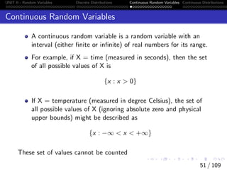
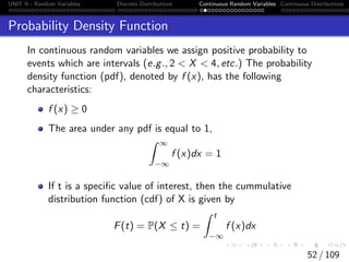
1) Discrete and continuous random variables and their probability mass functions (pmf) and probability density functions (pdf) respectively.
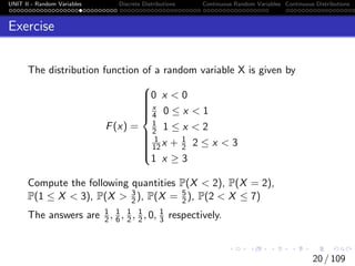
2) Computing probabilities of values a random variable can take using the pmf.
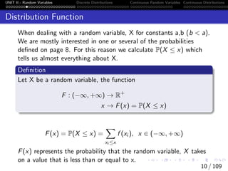
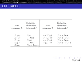
3) The cumulative distribution function (CDF) which gives the probability that a random variable is less than or equal to a value, and its properties.
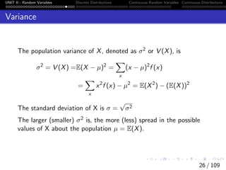
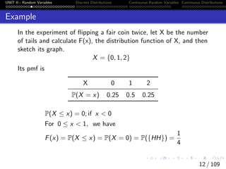
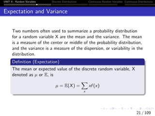
4) Expectation and variance as measures of a random variable's center and spread.
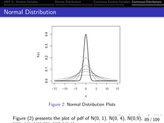
![UNIT II - Random Variables Discrete Distributions Continuous Random Variables Continuous Distributions
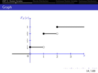
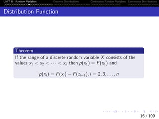
Properties of the CDF
(a) F(x) is non decreasing function of x (i.e if x ≤ y, then
F(x) ≤ F(y))
(b) lim
x→∞
F(x) = F(∞) = 1
(c) lim
x→−∞
F(x) = F(−∞) = 0
(d) P(x1 < X ≤ x2) = F(x2) − F(x1)
(e) For all x ∈ R we have P[X > x] = 1 − F(x)
11 / 109](https://image.slidesharecdn.com/stat253unitii-240328002652-4b9a18f7/85/STAT-253-Probability-and-Statistics-UNIT-II-pdf-11-320.jpg)
![UNIT II - Random Variables Discrete Distributions Continuous Random Variables Continuous Distributions
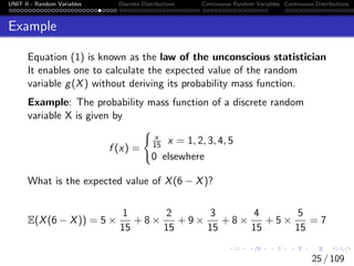
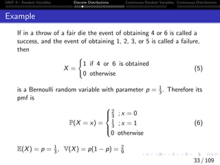
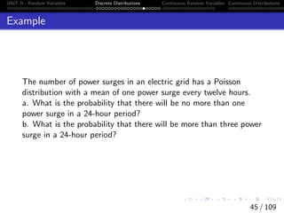
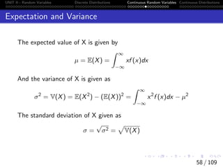
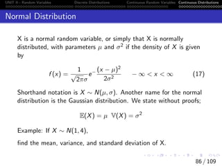
Expectation
Let X be a discrete random variable, then for any function
g : R → R, g(X) is also a discrete random variable and has
expectation
E(g(X)) =
X
∀x
g(x)f (x) (1)
Let a be a constant, then the following properties hold;
1
E(c) = c
2
E[cg(X)] = cE[g(X)]
23 / 109](https://image.slidesharecdn.com/stat253unitii-240328002652-4b9a18f7/85/STAT-253-Probability-and-Statistics-UNIT-II-pdf-23-320.jpg)
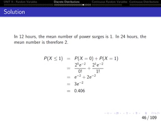
![UNIT II - Random Variables Discrete Distributions Continuous Random Variables Continuous Distributions
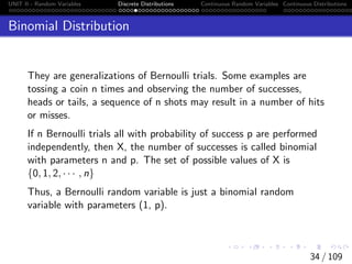
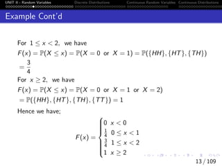
Expectation
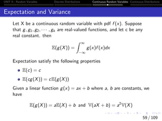
For linear function g(x) = ax +b where a, b are constants, we have
[3]E[g(X)] = aE(X) + b
We show proofs of [1], [2] and [3]. These rules are also applicable
if X is continuous.
24 / 109](https://image.slidesharecdn.com/stat253unitii-240328002652-4b9a18f7/85/STAT-253-Probability-and-Statistics-UNIT-II-pdf-24-320.jpg)