IUT Probability and Statistics - Chapter 02_Part-1.pdf
1.
Lecture 06 -
Chapter02: Random Variables
Math 4441: Probability and Statistics
Reference: Goodman & Yates – Introduction to Probability and Stochastic Process, 3rd
Edition
3.
Summary of Chapter1: Simple Probability Models
Sample Space: 𝑆
• Elements of 𝑆 can be anything
• Does not facilitate further processing
Probability of Outcomes/Events: 𝑝[⋅]
• Lack a concise Representation of probabilities
4.
Example 2.1: (Example1.12)
Procedure: Send 3 packets from a sender to a receiver.
Observation: Number of successes.
𝑆 = {𝐹𝐹𝐹, 𝐹𝐹𝐷, 𝐹𝐷𝐹, 𝐹𝐷𝐷, 𝐷𝐹𝐹, 𝐷𝐹𝐷, 𝐷𝐷𝐹, 𝐷𝐷𝐷}
Probabilities of Outcomes
𝑃[𝐹𝐹𝐹] = (1 − 𝑝)3
𝑃[𝐹𝐹𝐷] = 𝑝(1 − 𝑝)2
𝑃[𝐹𝐷𝐹] = 𝑝(1 − 𝑝)2
𝑃[𝐹𝐷𝐷] = 𝑝2
(1 − 𝑝)
𝑃[𝐷𝐹𝐹] = 𝑝(1 − 𝑝)2
𝑃[𝐷𝐹𝐷] = 𝑝2
(1 − 𝑝)
𝑃[𝐷𝐷𝐹] = 𝑝2
(1 − 𝑝)
𝑃[𝐹𝐷𝐷] = 𝑝3
𝑃[number of success is 0] = (1 − 𝑝)3
𝑃[number of success is 1] = 3𝑝(1 − 𝑝)2
𝑃[number of success is 2] = 3𝑝2
(1 − 𝑝)
𝑃[number of success is 3] = 𝑝3
𝑝 ≜ probability that a single packet is delivered
Each of the deliveries is independent of the others
5.
What do weneed?
• Each element of 𝑆 is a number
o Define a function that converts each element 𝜔 ∈ 𝑆 into a real
number 𝑥 ∈ 𝑅.
o 𝑋: 𝑆 → 𝑅
• Probabilities in a mathematical way
o Recalculate the probability of each real number or an interval of
numbers as outcome
o Represent both the real numbers and their probabilities
mathematically
7.
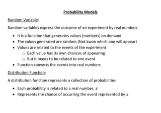
Probability Models
Random Variable:
Randomvariables express the outcome of an experiment by real numbers
• It is a function that generates values (numbers) on demand
• The values generated are random (Not kwon which one will appear)
• Values are related to the events of the experiment
o Each value has its own chances of appearing
o But it needs to be related to one event
• Function converts the events into real numbers
Distribution Function:
A distribution function represents a collection of probabilities
• Each probability is related to a real number, 𝑥
• Represents the chance of occurring the event represented by 𝑥
8.
Random Variable:
How todefine the functions?
• Identify the events related to the observations of the experiment
• Find an event space associated with the experiment (Why?)
• Assign a real number to each event – based on the problem statement
Type of Random Variables:
• Discrete random variables
o Possible values are from a discrete set
o Number of values are either finite or countably infinite
• Continuous random variables
o Possible values are from an interval
o Number of values are uncountable
• Mixed random variables
9.
Example 2.1: (Continued)
Procedure:Send 3 packets from a sender to a receiver.
Observation: Number of successes.
𝑆 = {𝐹𝐹𝐹, 𝐹𝐹𝐷, 𝐹𝐷𝐹, 𝐹𝐷𝐷, 𝐷𝐹𝐹, 𝐷𝐹𝐷, 𝐷𝐷𝐹, 𝐷𝐷𝐷}
Events related to the observations
𝐸𝑖 ≜ # of success(es) is 𝑖
𝑖 = 0, 1, … , 3
𝐸 = {𝐸0, 𝐸1, 𝐸2, 𝐸3}
𝑆𝑋 = { }
FFF
FFD
DDD
DDF
DFD
DFF
FDD
FDF
S
0
1
2
3
R
10.
Definition (Random Variable):The point function 𝑋(𝜔) is called a random variable
if
(a) It is a finite real-valued function defined on the sample space S of a random
experiment, and
(b) For every real number 𝑥, the set {𝜔: 𝑋(𝜔) ≤ 𝑥} is an event.
𝑋: 𝑆 → 𝑅
11.
Distributions Functions:
• Representsthe distribution of probabilities on the number line
• A probability is attached to each number on the number line
• Probabilities are non-zero for a number or an interval, only if the random
variable can take on that value
• Probability that 𝑥 is an outcome is related to the event corresponding to 𝑥
defined by the random variable
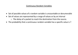
12.
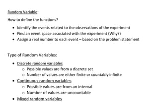
Probability Models byRandom Variables
Probability
Model
Random
Experiment
Sample Space (S)
Prob. of Event P[.]
Random Variable
X: S -> R
Real Numbers SX
{X <= s } is an event
Distribution
Function
P[X=x]
P[X<=x]
PX(x)
FX(x)
13.
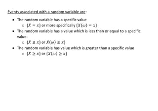
Events associated witha random variable are:
• The random variable has a specific value
o {𝑋 = 𝑥} or more specifically {𝑋(𝜔) = 𝑥}
• The random variable has a value which is less than or equal to a specific
value:
o {𝑋 ≤ 𝑥} or 𝑋(𝜔) ≤ 𝑥}
• The random variable has value which is greater than a specific value
o {𝑋 ≥ 𝑥} or {𝑋(𝜔) ≥ 𝑥}
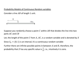
14.
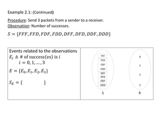
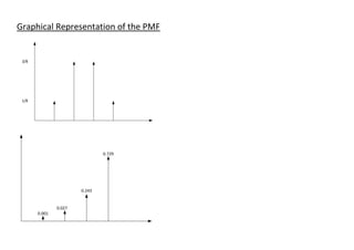
Possible distribution functionsare:
• Probability Mass function (PMF): The probability that a random variable 𝑋
has a specific value 𝑥
o 𝑃[𝑋 = 𝑥]
• Cumulative distribution function (CDF): The probability that a random
variable has a value which is less than or equal to a specific value 𝑥
o 𝑃[𝑋 ≤ 𝑥]
• Complementary cumulative distribution function (CCDF): The probability that
a random variable has a value which is greater than a specific value 𝑥
o 𝑃[𝑋 > 𝑥]
15.
Example 2.1: (Continued)
Procedure:Send 3 packets from a sender to a receiver.
Observation: Number of successes.
𝑆 = {𝐹𝐹𝐹, 𝐹𝐹𝐷, 𝐹𝐷𝐹, 𝐹𝐷𝐷, 𝐷𝐹𝐹, 𝐷𝐹𝐷, 𝐷𝐷𝐹, 𝐷𝐷𝐷}
𝐸 = {𝐸0, 𝐸1, 𝐸2, 𝐸3}
𝑋 ≜ Random variable that counts the number of successes
𝑆𝑋 = {0, 1, 2, 3}
𝐸0 𝐸1 𝐸2 𝐸3
𝑆 𝐹𝐹𝐹 𝐹𝐹𝐷 𝐹𝐷𝐹 𝐷𝐹𝐹 𝐹𝐷𝐷 𝐷𝐹𝐷 𝐷𝐷𝐹 𝐷𝐷𝐷
𝑥
𝑃[𝑋 = 𝑥]
𝑃[𝑋 ≤ 𝑥]
16.
Probability Mass Function(PMF): 𝑃𝑋(𝑥)
If the set of possible values of 𝑋, 𝑆𝑋 = {𝑥1, 𝑥2, … , 𝑥𝑛}, then
1. 𝑃𝑋(𝑥𝑖) = 0, if 𝑥𝑖 ∉ 𝑆𝑋
2. 𝑃𝑋(𝑥𝑖) = 𝑃[𝑋 = 𝑥𝑖], and hence, 𝑃𝑋(𝑥𝑖) > 0, for 𝑖 = 1, 2, … , 𝑛
3. ∑ 𝑃𝑋(𝑥𝑖) = 1
𝑛
𝑖
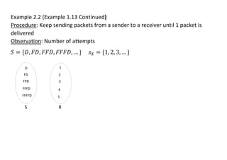
Example 2.2 (Example1.13 Continued)
Procedure: Keep sending packets from a sender to a receiver until 1 packet is
delivered
Observation: Number of attempts
𝑆 = {𝐷, 𝐹𝐷, 𝐹𝐹𝐷, 𝐹𝐹𝐹𝐷, … } 𝑠𝑋 = {1, 2, 3, … }
D
FD
FFFFD
FFFD
FFD
S
1
2
3
R
4
5
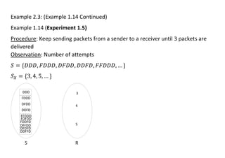
Example 2.3: (Example1.14 Continued)
Example 1.14 (Experiment 1.5)
Procedure: Keep sending packets from a sender to a receiver until 3 packets are
delivered
Observation: Number of attempts
𝑆 = {𝐷𝐷𝐷, 𝐹𝐷𝐷𝐷, 𝐷𝐹𝐷𝐷, 𝐷𝐷𝐹𝐷, 𝐹𝐹𝐷𝐷𝐷, … }
𝑆𝑋 = {3, 4, 5, … }
DDD
FDDD
FDDFD
FDFDD
FFDDD
DDFD
DFDD
S
3
4
5
R
DFFDD
DFDFD
DDFFD
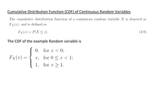
Cumulative Distribution Function(CDF)
𝐹𝑋(𝑥) = 𝑃[𝑋 ≤ 𝑥]
Probability that 𝑋 will assume a value from the subset of 𝑆, where the subset is
the point 𝑥 and all the points to the left of 𝑥.
26.
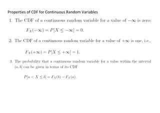
Properties of CDF:
1.It is applicable to both discrete and continuous RVs
2. It is nonnegative, non-decreasing function of 𝑥
3. For discreate random variables it is step function
a. Jumps at the values of 𝑥 where 𝑃𝑋(𝑥) > 0
b. For continuous random variables, it is continuous
4.
a. 𝐹𝑋(−∞) = 0
b. 𝐹𝑋(+∞) = 1
5. If 𝑎 and 𝑏 are two real numbers such that 𝑎 < 𝑏
𝑃[𝑎 < 𝑋 ≤ 𝑏] = 𝐹𝑋(𝑏) − 𝐹𝑋(𝑎)
Which is a direct result of
𝑃[𝑋 ≤ 𝑏] = 𝑃[𝑋 ≤ 𝑧] + 𝑃[𝑎 < 𝑋 ≤ 𝑏]
27.
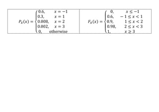
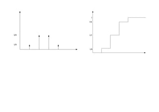
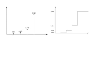
Example 2.4: Leta discrete random variable 𝑋 assumes values −1, 1, 2, and 3, with
probabilities 0.6, 0.3, 0.08, and 0.02 , respectively.
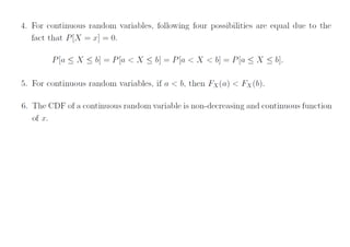
Continuous Random Variables
•Set of possible values of a random variable is uncountable or denumerable
• Set of values are represented by a range of values or by an interval
o The delay of a packet to reach the destination from the source.
• The probability that a continuous random variable has a specific value is ?
32.
Probability Models ofContinuous Random variables
Consider a line 𝐴𝐵 of length 1 unit.
Suppose you randomly choose a point 𝐶 within 𝐴𝐵 that divides the line into two
parts 𝐴𝐶 and 𝐶𝐵
Let, the length of the point 𝐶 from 𝐴, 𝐴𝐶, is a random variable and is denoted by 𝑋
Since 𝑆𝑋 = (0, 1) is an interval, X is a continuous random variable
Further there are infinite possible points in between 𝐴 and 𝐵, therefore, the
probability that 𝑋 has any specific value is
1
∞
, i.e., intuitively it is zero.
33.
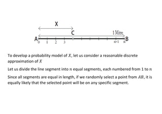
To develop aprobability model of 𝑋, let us consider a reasonable discrete
approximation of 𝑋
Let us divide the line segment into 𝑛 equal segments, each numbered from 1 to 𝑛
Since all segments are equal in length, if we randomly select a point from 𝐴𝐵, it is
equally likely that the selected point will be on any specific segment.
34.
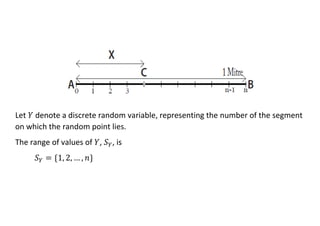
Let 𝑌 denotea discrete random variable, representing the number of the segment
on which the random point lies.
The range of values of 𝑌, 𝑆𝑌, is
𝑆𝑌 = {1, 2, … , 𝑛}
35.
Two important questionsto be answered are:
1. The relation between random variable 𝑋 and the random variable 𝑌
2. How well does 𝑌 approximate the value of 𝑋.
From the Figure, we can easily see that
𝑌 = ⌈𝑛𝑋⌉
If we denote {𝑋 = 𝑥} and {𝑌 = ⌈𝑛𝑋⌉} as two events, we have
{𝑋 = 𝑥} ⊂ {𝑌 = ⌈𝑛𝑋⌉}, and it implies
𝑃[𝑋 = 𝑥] ≤ 𝑃[𝑌 = ⌈𝑛𝑋⌉] = 𝑃[𝑋 = 𝑥] ≤
1
𝑛
𝑃[𝑋 = 𝑥] ≤ lim
𝑛→∞
𝑃[𝑌 = ⌈𝑛𝑋⌉ = lim
𝑛→∞
1
𝑛
= 0
𝑃[𝑋 = 𝑥] ≤ 0
However, according to the 1st Axioms of Probability 𝑃[𝑋 = 𝑥] ≥ 0, hence
𝑃[𝑋 = 𝑥] = 0
36.
PMF as aProbability Model for Continuous Random Variables:
Since 𝑃𝑋(𝑥) = 𝑃[𝑋 = 𝑥] and 𝑃[𝑋 = 𝑥] = 0 for continuous random variables,
• The probability that a continuous RV has a specific value is always zero.
• The MPF is meaningless for a continuous random variable.
37.
Distribution Functions forContinuous Random Variables
• The probability of a continuous random variable for a specific value is not
defined.
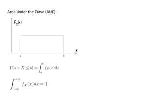
• However, probability for a range of values, an interval, is well defined
o 𝑃[𝑎 < 𝑋 ≤ 𝑏] is well defined
• All points in [0,1] are equally likely to be selected as point 𝐶
• Assume 𝑎 = 0 and 𝑐 = 0.5, intuitively we can say that 50% of the time point
𝐶 will be selected in the interval [0, 0.5]
• Probability that 𝑋 has a value between 0 and 0.5 is
𝑃[𝑎 < 𝑋 ≤ 𝑏] = 𝑃[0 < 𝑋 ≤ 0.5] =
0.5
1.0
= 0.5
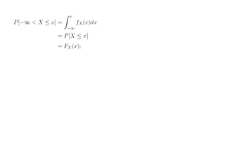
• Further assume that 𝑎 = ∞ and 𝑏 = 𝑥 then
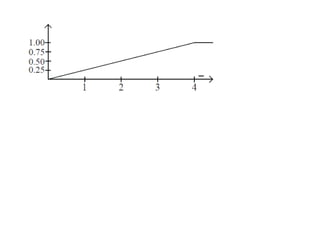
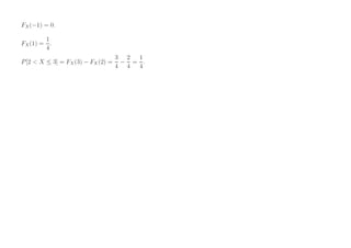
Example 2. 10:The CDF of a continuous random variable is
a) Draw the CDF curve.
b) Find the values of 𝐹𝑋(−1), 𝐹𝑋(1), 𝑃[2 < 𝑋 ≤ 3] and 𝐹𝑋(1.5).
44.
Probability Density Function(PDF)
• PMF: Distribution of probabilities (one unit) on the number line
For continuous Random variable defined in (0, 1)
• Distribute one unit of probability in the interval [0, 1] on the number line
• Infinite points, cannot assign probability to a specific point, 𝑃[𝑋 = 𝑥] = 0
• Though, can assign probability for a range of values, e.g., 0.25 unit in [0,0.25]
0.50 unit in [0, 0.50]
• Distribution can be uniform or non-uniform
We lack to quantify the amount of probability for a specific value of 𝑋
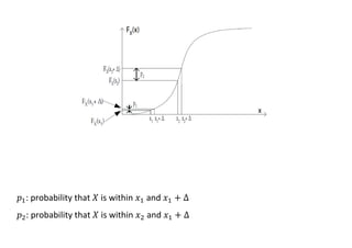
46.
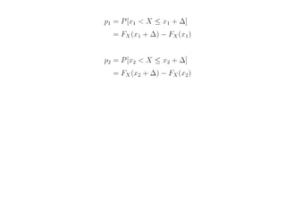
𝑝1: probability that𝑋 is within 𝑥1 and 𝑥1 + Δ
𝑝2: probability that 𝑋 is within 𝑥2 and 𝑥1 + Δ
49.
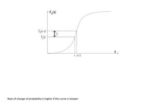
Rate of changeof probability is higher if the curve is steeper
50.
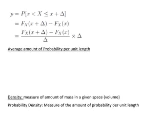
Average amount ofProbability per unit length
Density: measure of amount of mass in a given space (volume)
Probability Density: Measure of the amount of probability per unit length
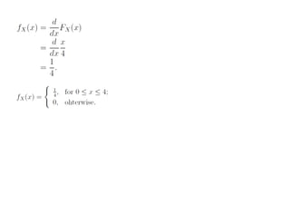
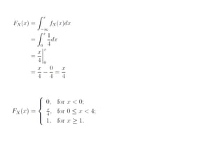
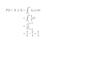
Example 2.11: Forthe CDF 𝐹𝑋(𝑥) given in Example 3.11, find the following:
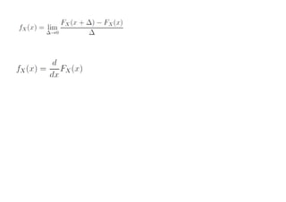
1. 𝑓𝑋(𝑥), from the CDF
2. 𝐹𝑋(𝑥), from the PDF
3. 𝑃[2 < 𝑋 ≤ 3] =?
4. Draw the PDF curve

![Summary of Chapter 1: Simple Probability Models
Sample Space: 𝑆
• Elements of 𝑆 can be anything
• Does not facilitate further processing
Probability of Outcomes/Events: 𝑝[⋅]
• Lack a concise Representation of probabilities](https://image.slidesharecdn.com/chapter02part-1-250702201347-e4a3e26b/85/IUT-Probability-and-Statistics-Chapter-02_Part-1-pdf-3-320.jpg)
![Example 2.1: (Example 1.12)
Procedure: Send 3 packets from a sender to a receiver.
Observation: Number of successes.
𝑆 = {𝐹𝐹𝐹, 𝐹𝐹𝐷, 𝐹𝐷𝐹, 𝐹𝐷𝐷, 𝐷𝐹𝐹, 𝐷𝐹𝐷, 𝐷𝐷𝐹, 𝐷𝐷𝐷}
Probabilities of Outcomes
𝑃[𝐹𝐹𝐹] = (1 − 𝑝)3
𝑃[𝐹𝐹𝐷] = 𝑝(1 − 𝑝)2
𝑃[𝐹𝐷𝐹] = 𝑝(1 − 𝑝)2
𝑃[𝐹𝐷𝐷] = 𝑝2
(1 − 𝑝)
𝑃[𝐷𝐹𝐹] = 𝑝(1 − 𝑝)2
𝑃[𝐷𝐹𝐷] = 𝑝2
(1 − 𝑝)
𝑃[𝐷𝐷𝐹] = 𝑝2
(1 − 𝑝)
𝑃[𝐹𝐷𝐷] = 𝑝3
𝑃[number of success is 0] = (1 − 𝑝)3
𝑃[number of success is 1] = 3𝑝(1 − 𝑝)2
𝑃[number of success is 2] = 3𝑝2
(1 − 𝑝)
𝑃[number of success is 3] = 𝑝3
𝑝 ≜ probability that a single packet is delivered
Each of the deliveries is independent of the others](https://image.slidesharecdn.com/chapter02part-1-250702201347-e4a3e26b/85/IUT-Probability-and-Statistics-Chapter-02_Part-1-pdf-4-320.jpg)

![Probability Models by Random Variables
Probability
Model
Random
Experiment
Sample Space (S)
Prob. of Event P[.]
Random Variable
X: S -> R
Real Numbers SX
{X <= s } is an event
Distribution
Function
P[X=x]
P[X<=x]
PX(x)
FX(x)](https://image.slidesharecdn.com/chapter02part-1-250702201347-e4a3e26b/85/IUT-Probability-and-Statistics-Chapter-02_Part-1-pdf-12-320.jpg)
![Possible distribution functions are:
• Probability Mass function (PMF): The probability that a random variable 𝑋
has a specific value 𝑥
o 𝑃[𝑋 = 𝑥]
• Cumulative distribution function (CDF): The probability that a random
variable has a value which is less than or equal to a specific value 𝑥
o 𝑃[𝑋 ≤ 𝑥]
• Complementary cumulative distribution function (CCDF): The probability that
a random variable has a value which is greater than a specific value 𝑥
o 𝑃[𝑋 > 𝑥]](https://image.slidesharecdn.com/chapter02part-1-250702201347-e4a3e26b/85/IUT-Probability-and-Statistics-Chapter-02_Part-1-pdf-14-320.jpg)
![Example 2.1: (Continued)
Procedure: Send 3 packets from a sender to a receiver.
Observation: Number of successes.
𝑆 = {𝐹𝐹𝐹, 𝐹𝐹𝐷, 𝐹𝐷𝐹, 𝐹𝐷𝐷, 𝐷𝐹𝐹, 𝐷𝐹𝐷, 𝐷𝐷𝐹, 𝐷𝐷𝐷}
𝐸 = {𝐸0, 𝐸1, 𝐸2, 𝐸3}
𝑋 ≜ Random variable that counts the number of successes
𝑆𝑋 = {0, 1, 2, 3}
𝐸0 𝐸1 𝐸2 𝐸3
𝑆 𝐹𝐹𝐹 𝐹𝐹𝐷 𝐹𝐷𝐹 𝐷𝐹𝐹 𝐹𝐷𝐷 𝐷𝐹𝐷 𝐷𝐷𝐹 𝐷𝐷𝐷
𝑥
𝑃[𝑋 = 𝑥]
𝑃[𝑋 ≤ 𝑥]](https://image.slidesharecdn.com/chapter02part-1-250702201347-e4a3e26b/85/IUT-Probability-and-Statistics-Chapter-02_Part-1-pdf-15-320.jpg)
![Probability Mass Function (PMF): 𝑃𝑋(𝑥)
If the set of possible values of 𝑋, 𝑆𝑋 = {𝑥1, 𝑥2, … , 𝑥𝑛}, then
1. 𝑃𝑋(𝑥𝑖) = 0, if 𝑥𝑖 ∉ 𝑆𝑋
2. 𝑃𝑋(𝑥𝑖) = 𝑃[𝑋 = 𝑥𝑖], and hence, 𝑃𝑋(𝑥𝑖) > 0, for 𝑖 = 1, 2, … , 𝑛
3. ∑ 𝑃𝑋(𝑥𝑖) = 1
𝑛
𝑖](https://image.slidesharecdn.com/chapter02part-1-250702201347-e4a3e26b/85/IUT-Probability-and-Statistics-Chapter-02_Part-1-pdf-16-320.jpg)

![𝐸1 𝐸2 𝐸3 𝐸4 𝐸5
𝑆 𝐷 𝐹𝐷 𝐹𝐹𝐷 𝐹𝐹𝐹𝐷 𝐹𝐹𝐹𝐹𝐷
𝑥
𝑃[𝑋 = 𝑥]
𝑃[𝑋 ≤ 𝑥]
𝐹𝑋(𝑥) = 1 − (1 − 𝑝)𝑥
𝑥 ≥ 1](https://image.slidesharecdn.com/chapter02part-1-250702201347-e4a3e26b/85/IUT-Probability-and-Statistics-Chapter-02_Part-1-pdf-21-320.jpg)

![𝐸3 𝐸4 𝐸5
𝑆 𝐷𝐷𝐷 𝐹𝐷𝐷𝐷 𝐷𝐹𝐷𝐷 𝐷𝐷𝐹𝐷 𝐹𝐹𝐷𝐷𝐷 𝐹𝐷𝐹𝐷𝐷 𝐹𝐷𝐷𝐹𝐷
𝐷𝐹𝐹𝐷𝐷, 𝐷𝐹𝐷𝐹𝐷, 𝐷𝐷𝐹𝐹𝐷
𝑥
𝑃[𝑋 = 𝑥]
𝑃[𝑋 ≤ 𝑥]](https://image.slidesharecdn.com/chapter02part-1-250702201347-e4a3e26b/85/IUT-Probability-and-Statistics-Chapter-02_Part-1-pdf-24-320.jpg)
![Cumulative Distribution Function (CDF)
𝐹𝑋(𝑥) = 𝑃[𝑋 ≤ 𝑥]
Probability that 𝑋 will assume a value from the subset of 𝑆, where the subset is
the point 𝑥 and all the points to the left of 𝑥.](https://image.slidesharecdn.com/chapter02part-1-250702201347-e4a3e26b/85/IUT-Probability-and-Statistics-Chapter-02_Part-1-pdf-25-320.jpg)
![Properties of CDF:
1. It is applicable to both discrete and continuous RVs
2. It is nonnegative, non-decreasing function of 𝑥
3. For discreate random variables it is step function
a. Jumps at the values of 𝑥 where 𝑃𝑋(𝑥) > 0
b. For continuous random variables, it is continuous
4.
a. 𝐹𝑋(−∞) = 0
b. 𝐹𝑋(+∞) = 1
5. If 𝑎 and 𝑏 are two real numbers such that 𝑎 < 𝑏
𝑃[𝑎 < 𝑋 ≤ 𝑏] = 𝐹𝑋(𝑏) − 𝐹𝑋(𝑎)
Which is a direct result of
𝑃[𝑋 ≤ 𝑏] = 𝑃[𝑋 ≤ 𝑧] + 𝑃[𝑎 < 𝑋 ≤ 𝑏]](https://image.slidesharecdn.com/chapter02part-1-250702201347-e4a3e26b/85/IUT-Probability-and-Statistics-Chapter-02_Part-1-pdf-26-320.jpg)

![Two important questions to be answered are:
1. The relation between random variable 𝑋 and the random variable 𝑌
2. How well does 𝑌 approximate the value of 𝑋.
From the Figure, we can easily see that
𝑌 = ⌈𝑛𝑋⌉
If we denote {𝑋 = 𝑥} and {𝑌 = ⌈𝑛𝑋⌉} as two events, we have
{𝑋 = 𝑥} ⊂ {𝑌 = ⌈𝑛𝑋⌉}, and it implies
𝑃[𝑋 = 𝑥] ≤ 𝑃[𝑌 = ⌈𝑛𝑋⌉] = 𝑃[𝑋 = 𝑥] ≤
1
𝑛
𝑃[𝑋 = 𝑥] ≤ lim
𝑛→∞
𝑃[𝑌 = ⌈𝑛𝑋⌉ = lim
𝑛→∞
1
𝑛
= 0
𝑃[𝑋 = 𝑥] ≤ 0
However, according to the 1st Axioms of Probability 𝑃[𝑋 = 𝑥] ≥ 0, hence
𝑃[𝑋 = 𝑥] = 0](https://image.slidesharecdn.com/chapter02part-1-250702201347-e4a3e26b/85/IUT-Probability-and-Statistics-Chapter-02_Part-1-pdf-35-320.jpg)
![PMF as a Probability Model for Continuous Random Variables:
Since 𝑃𝑋(𝑥) = 𝑃[𝑋 = 𝑥] and 𝑃[𝑋 = 𝑥] = 0 for continuous random variables,
• The probability that a continuous RV has a specific value is always zero.
• The MPF is meaningless for a continuous random variable.](https://image.slidesharecdn.com/chapter02part-1-250702201347-e4a3e26b/85/IUT-Probability-and-Statistics-Chapter-02_Part-1-pdf-36-320.jpg)
![Distribution Functions for Continuous Random Variables
• The probability of a continuous random variable for a specific value is not
defined.
• However, probability for a range of values, an interval, is well defined
o 𝑃[𝑎 < 𝑋 ≤ 𝑏] is well defined
• All points in [0,1] are equally likely to be selected as point 𝐶
• Assume 𝑎 = 0 and 𝑐 = 0.5, intuitively we can say that 50% of the time point
𝐶 will be selected in the interval [0, 0.5]
• Probability that 𝑋 has a value between 0 and 0.5 is
𝑃[𝑎 < 𝑋 ≤ 𝑏] = 𝑃[0 < 𝑋 ≤ 0.5] =
0.5
1.0
= 0.5
• Further assume that 𝑎 = ∞ and 𝑏 = 𝑥 then](https://image.slidesharecdn.com/chapter02part-1-250702201347-e4a3e26b/85/IUT-Probability-and-Statistics-Chapter-02_Part-1-pdf-37-320.jpg)
![Example 2. 10: The CDF of a continuous random variable is
a) Draw the CDF curve.
b) Find the values of 𝐹𝑋(−1), 𝐹𝑋(1), 𝑃[2 < 𝑋 ≤ 3] and 𝐹𝑋(1.5).](https://image.slidesharecdn.com/chapter02part-1-250702201347-e4a3e26b/85/IUT-Probability-and-Statistics-Chapter-02_Part-1-pdf-41-320.jpg)
![Probability Density Function (PDF)
• PMF: Distribution of probabilities (one unit) on the number line
For continuous Random variable defined in (0, 1)
• Distribute one unit of probability in the interval [0, 1] on the number line
• Infinite points, cannot assign probability to a specific point, 𝑃[𝑋 = 𝑥] = 0
• Though, can assign probability for a range of values, e.g., 0.25 unit in [0,0.25]
0.50 unit in [0, 0.50]
• Distribution can be uniform or non-uniform
We lack to quantify the amount of probability for a specific value of 𝑋](https://image.slidesharecdn.com/chapter02part-1-250702201347-e4a3e26b/85/IUT-Probability-and-Statistics-Chapter-02_Part-1-pdf-44-320.jpg)


![Example 2.11: For the CDF 𝐹𝑋(𝑥) given in Example 3.11, find the following:
1. 𝑓𝑋(𝑥), from the CDF
2. 𝐹𝑋(𝑥), from the PDF
3. 𝑃[2 < 𝑋 ≤ 3] =?
4. Draw the PDF curve](https://image.slidesharecdn.com/chapter02part-1-250702201347-e4a3e26b/85/IUT-Probability-and-Statistics-Chapter-02_Part-1-pdf-54-320.jpg)