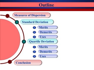
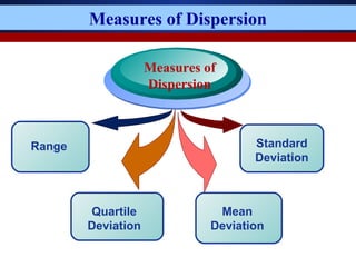
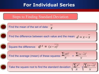
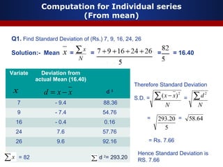
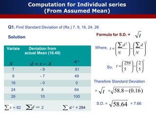
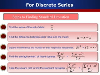
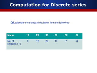
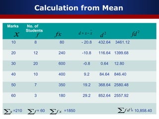
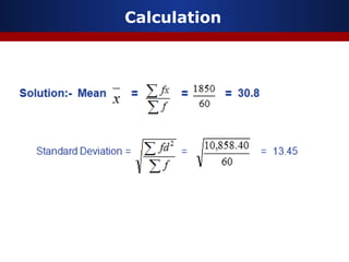
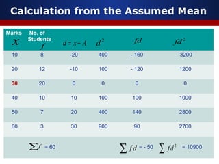
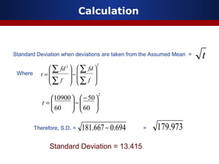
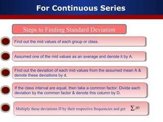
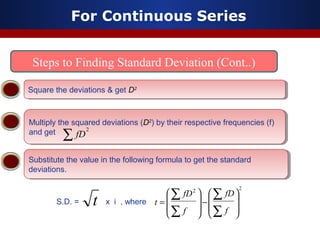
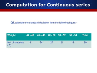
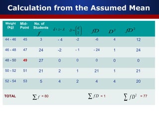
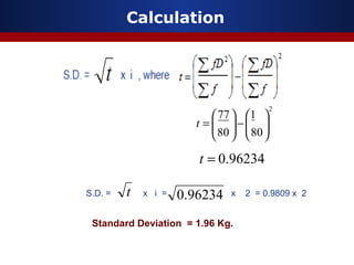
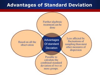
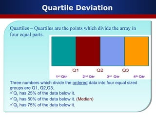
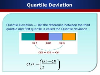
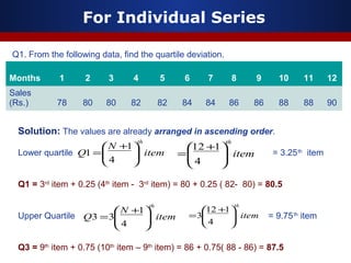
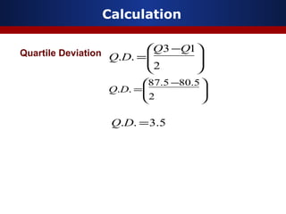
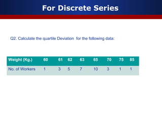
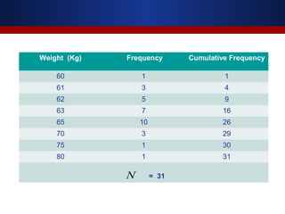
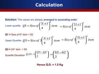
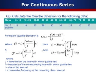
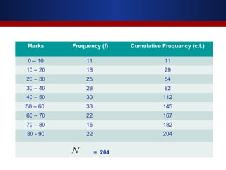
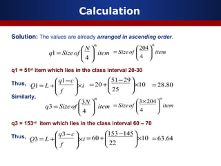
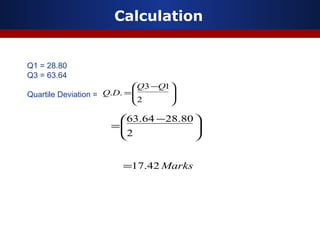
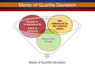
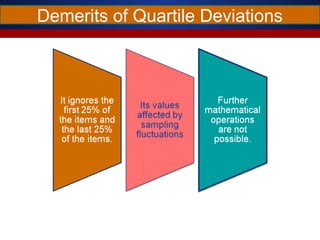
Measures of Dispersion- Standard
deviation & Quartile Deviation
Measures of Dispersion- Standard
deviation & Quartile Deviation
Rekha Yadav
Faculty of Education,
Dayalbagh Educational Institute
Dayalbagh, Agra.
March 31, 2015
Measures of DispersionMeasures of Dispersion
Outline
Standard DeviationStandard Deviation
MeritsMerits
DemeritsDemerits
UsesUses
Quartile DeviationQuartile Deviation
MeritsMerits
DemeritsDemerits
UsesUses
ConclusionConclusion
Measures of Dispersion
The measurement of scattered-ness of the mass of
figures in a series about an average is called measure of
dispersion or measure of variation.
In two or more distributions the central value may be the
same but still there can be wide disparities in the
formation of the distribution. Measures of dispersion
helps in studying this important characteristics of a
distribution.
Range
Measures of
Dispersion
Measures of Dispersion
Quartile
Deviation
Standard
Deviation
Mean
Deviation
Standard DeviationStandard Deviation
Standard Deviation
The standard deviation concept was introduced by Karl Pearson
in 1893.
It is most important & widely used measures of dispersion.
Standard deviation is also known as root mean square
deviation for the reason that it is the square root of the mean of
the squared deviation from the arithmetic mean.
Standard deviation is denoted by the Greek letter σ (read as
sigma)
The value of the standard deviation tells how closely the
values of a data set are clustered around the mean.
Method of calculation of
Standard Deviation
Method of calculation of
Standard Deviation
Types of Series
Enc
Series
Continuous
Series
Discrete
Series
Individual
series
For Individual Series
Steps to Finding Standard Deviation
Find the mean of the set of data:Find the mean of the set of data:
Find the difference between each value and the mean:Find the difference between each value and the mean:
x
Square the difference:Square the difference:
Find the average (mean) of these squares:Find the average (mean) of these squares:
N
xx∑ − 2
)(
Take the square root to find the standard deviation:Take the square root to find the standard deviation:
N
xx∑ − 2
)(
2
)( xx −
xx −
Find the mean of the set of data:Find the mean of the set of data:
Find the difference between each value and the mean:Find the difference between each value and the mean:
x
Square the difference:Square the difference:
Find the average (mean) of these squares: =Find the average (mean) of these squares: =
N
xx∑ − 2
)(
Take the square root to find the standard deviation: =Take the square root to find the standard deviation: =
N
xx∑ − 2
)(
xxd −=
d 2
= 2
)( xx −
N
d∑ 2
N
d∑ 2
)(
Computation for Individual series
(From mean)
Q1. Find Standard Deviation of (Rs.) 7, 9, 16, 24, 26
Solution:- Mean = = = = 16.40
Variate Deviation from
actual Mean (16.40)
d 2
7 - 9.4 88.36
9 - 7.4 54.76
16 - 0.4 0.16
24 7.6 57.76
26 9.6 92.16
= 82 d 2
= 293.20
x
N
x∑
xxd −=
N
d∑ 2
N
xx∑ − 2
)(
Therefore Standard Deviation
S.D. = =
= =
5
20.293 64.58
= Rs. 7.66
Hence Standard Deviation is
RS. 7.66
x
Computation for Individual series
(From Assumed Mean)
Q1. Find Standard Deviation of (Rs.) 7, 9, 16, 24, 26
Solution
Variate Deviation from
actual Mean (16.40)
d 2
7 - 9 81
9 - 7 49
16 - 0 0
24 8 64
26 10 100
= 82 2 d 2
= 294
x Axd −=
Formula for S.D. = t
Where,
22








−








=
∑∑
N
d
N
d
t
So,
2
5
2
5
294






−





=t
Therefore Standard Deviation
= =
64.58
)16.0(8.58 −
S.D. = = 7.66
t
∑ =d
For Discrete Series
Steps to Finding Standard Deviation
Find the mean of the set of data:Find the mean of the set of data:
Find the difference between each value and the mean:Find the difference between each value and the mean:
x
Square the difference and multiply by their respective frequencies: =Square the difference and multiply by their respective frequencies: =
Find the average (mean) of these squares: =Find the average (mean) of these squares: =
∑
∑ −
f
xxf 2
)(
Take the square root to find the standard deviation: =Take the square root to find the standard deviation: =
∑
∑ −
f
xxf 2
)(
xxd −=
2
)( xxf −
∑
∑
f
fd 2
∑
∑
f
fd 2
2
fd
Computation for Discrete series
Q1.calculate the standard deviation from the following:-
Marks 10 20 30 30 50 60
No. of
students ( f )
8 12 20 10 7 3
Calculation from Mean
Marks No. of
Students
10 8 80 - 20.8 432.64 3461.12
20 12 240 -10.8 116.64 1399.68
30 20 600 -0.8 0.64 12.80
40 10 400 9.2 84.64 846.40
50 7 350 19.2 368.64 2580.48
60 3 180 29.2 852.64 2557.92
=210 = 60 =1850 = 10,858.40
f fx xxd −= 2
fd2
d
∑x
x
∑f xf∑
2
df∑
Calculation
Calculation from the Assumed Mean
Marks No. of
Students
10 8 -20 400 - 160 3200
20 12 -10 100 - 120 1200
30 20 0 0 0 0
40 10 10 100 100 1000
50 7 20 400 140 2800
60 3 30 900 90 2700
= 60 = - 50 = 10900
f Axd −= 2
dx
∑f 2
df∑
fd 2
fd
df∑
Calculation
Standard Deviation when deviations are taken from the Assumed Mean =
22








−








=
∑
∑
∑
∑
f
fd
f
fd
t
694.0667.181 −
Where
Therefore, S.D. = =
2
60
50
60
10900





−
−





=t
973.179
Standard Deviation = 13.415
t
For Continuous Series
Steps to Finding Standard Deviation
Find out the mid values of each group or class.Find out the mid values of each group or class.
Assumed one of the mid values as an average and denote it by A.Assumed one of the mid values as an average and denote it by A.
Find out the deviation of each mid values from the assumed mean A &
denote these deviations by d.
Find out the deviation of each mid values from the assumed mean A &
denote these deviations by d.
If the class interval are equal, then take a common factor. Divide each
deviation by the common factor & denote this column by D.
If the class interval are equal, then take a common factor. Divide each
deviation by the common factor & denote this column by D.
Multiply these deviations D by their respective frequencies and getMultiply these deviations D by their respective frequencies and get ∑ fD
For Continuous Series
Steps to Finding Standard Deviation (Cont..)
Multiply the squared deviations (D2
) by their respective frequencies (f)
and get
Multiply the squared deviations (D2
) by their respective frequencies (f)
and get
Substitute the value in the following formula to get the standard
deviations.
Substitute the value in the following formula to get the standard
deviations.
Square the deviations & get D2Square the deviations & get D2
2
∑ fD
S.D. = x i , wheret
22








−








=
∑
∑
∑
∑
f
fD
f
fD
t
Computation for Continuous series
Q1.calculate the standard deviation from the following figure:-
Weight 44 - 46 46 – 48 48 - 50 50 - 52 52 - 54 Total
No. of students
( f )
3 24 27 21 5 80
Calculation from the Assumed Mean
Weight
(kg)
Mid-
Point
No. of
Students
44 - 46 45 3 - 4 -2 -6 4 12
46 - 48 47 24 -2 - 1 - 24 1 24
48 - 50 49 27 0 0 0 0 0
50 - 52 51 21 2 1 21 1 21
52 - 54 53 5 4 2 4 4 20
TOTAL = 80 = 1 = 77
f
Axd −= 





=
2
d
D
∑ f
2
Df∑
fD
2
fD
Df∑
2
D
Calculation
2
80
1
80
77






−





=t
96234.0S.D. = x i = x 2 = 0.9809 x 2t
96234.0=t
Standard Deviation = 1.96 Kg.
Advantages of Standard Deviation
Demerits
Uses
Quartile DeviationQuartile Deviation
Quartile Deviation
Quartiles – Quartiles are the points which divide the array in
four equal parts.
Three numbers which divide the ordered data into four equal sized
groups are Q1, Q2,Q3.
Q1 has 25% of the data below it.
Q2 has 50% of the data below it. (Median)
Q3 has 75% of the data below it.
Quartiles – Quartiles are the points which divide the array in
four equal parts.
Three numbers which divide the ordered data into four equal sized
groups are Q1, Q2,Q3.
Q1 has 25% of the data below it.
Q2 has 50% of the data below it. (Median)
Q3 has 75% of the data below it.
Quartile Deviation
Quartile Deviation – Half the difference between the third
quartile and first quartile is called the Quartile deviation.
Quartile Deviation – Half the difference between the third
quartile and first quartile is called the Quartile deviation.







 −
=
2
13
..
QQ
DQ
Method of calculation of
Quartile Deviation
Method of calculation of
Quartile Deviation
For Individual Series
Q1. From the following data, find the quartile deviation.
Months 1 2 3 4 5 6 7 8 9 10 11 12
Sales
(Rs.) 78 80 80 82 82 84 84 86 86 88 88 90
Solution: The values are already arranged in ascending order.
Lower quartile = 3.25th
item
Q1 = 3rd
item + 0.25 (4th
item - 3rd
item) = 80 + 0.25 ( 82- 80) = 80.5
Upper Quartile = 9.75th
item
Q3 = 9th
item + 0.75 (10th
item – 9th
item) = 86 + 0.75( 88 - 86) = 87.5
item
N
Q
th





 +
=
4
1
1
item
N
Q
th





 +
=
4
1
33
item
th





 +
=
4
112
item
th





 +
=
4
112
3
Calculation
Quartile Deviation







 −
=
2
13
..
QQ
DQ





 −
=
2
5.805.87
..DQ
5.3.. =DQ
For Discrete Series
Weight (Kg.) 60 61 62 63 65 70 75 85
No. of Workers 1 3 5 7 10 3 1 1
Q2. Calculate the quartile Deviation for the following data:
Weight (Kg) Frequency Cumulative Frequency
60 1 1
61 3 4
62 5 9
63 7 16
65 10 26
70 3 29
75 1 30
80 1 31
= 31N
Calculation
Solution: The values are already arranged in ascending order.
Lower quartile
Q1 = Size of 8th
item = 62
Upper Quartile
Q3 = 24th
item = 65
Quartile Deviation
Hence Q.D. = 1.5 Kg
item
N
ofSizeQ
th





 +
=
4
1
1 itemofSize
th





 +
=
4
131
itemofSize
th





 +
=
4
131
3item
N
ofSizeQ
th





 +
=
4
1
33





 −
=
2
6265







 −
=
2
13
..
QQ
DQ
For Continuous Series
Q3. Calculate the Quartile deviation for the following data:
Marks 0 - 10 10 - 20 20-30 30 - 40 40 - 50 50 - 60 60 - 70 70 - 80 80 - 90
No. of
Students
11 18 25 28 30 33 22 15 22
Formula of Quartile Deviation is
Where , Here
& , here
where
L = lower limit of the interval in which quartile lies.
f = frequency of the corresponding interval in which quartile lies
i = size of the interval
c = cumulative frequency of the preceding class interval







 −
=
2
13
..
QQ
DQ
i
f
cq
LQ ×






 −
+=
1
1 item
N
ofSizeq
th






=
4
1
i
f
cq
LQ ×






 −
+=
3
3 item
N
ofSizeq
th






=
4
3
3
Marks Frequency (f) Cumulative Frequency (c.f.)
0 – 10 11 11
10 – 20 18 29
20 – 30 25 54
30 – 40 28 82
40 – 50 30 112
50 – 60 33 145
60 – 70 22 167
70 – 80 15 182
80 - 90 22 204
= 204N
Calculation
Solution: The values are already arranged in ascending order.
q1 = 51st
item which lies in the class interval 20-30
Thus,
Similarly,
q3 = 153rd
item which lies in the class interval 60 – 70
Thus,
item
N
ofSizeq
th






=
4
1 itemofSize
th






=
4
204
i
f
cq
LQ ×






 −
+=
1
1 10
25
2951
20 ×




 −
+= 80.28=
item
N
ofSizeq
th






=
4
3
3 itemofSize
th





 ×
=
4
2043
i
f
cq
LQ ×






 −
+=
3
3 10
22
145153
60 ×




 −
+= 64.63=
Calculation
Q1 = 28.80
Q3 = 63.64
Quartile Deviation = 






 −
=
2
13
..
QQ
DQ





 −
=
2
80.2864.63
Marks42.17=
Merits of Quartile Deviation
Demerits of Quartile Deviations
QUESTIONS

Standard deviation quartile deviation

  • 1.
    Measures of Dispersion-Standard deviation & Quartile Deviation Measures of Dispersion- Standard deviation & Quartile Deviation Rekha Yadav Faculty of Education, Dayalbagh Educational Institute Dayalbagh, Agra. March 31, 2015
  • 2.
    Measures of DispersionMeasuresof Dispersion Outline Standard DeviationStandard Deviation MeritsMerits DemeritsDemerits UsesUses Quartile DeviationQuartile Deviation MeritsMerits DemeritsDemerits UsesUses ConclusionConclusion
  • 3.
    Measures of Dispersion Themeasurement of scattered-ness of the mass of figures in a series about an average is called measure of dispersion or measure of variation. In two or more distributions the central value may be the same but still there can be wide disparities in the formation of the distribution. Measures of dispersion helps in studying this important characteristics of a distribution.
  • 4.
    Range Measures of Dispersion Measures ofDispersion Quartile Deviation Standard Deviation Mean Deviation
  • 5.
  • 6.
    Standard Deviation The standarddeviation concept was introduced by Karl Pearson in 1893. It is most important & widely used measures of dispersion. Standard deviation is also known as root mean square deviation for the reason that it is the square root of the mean of the squared deviation from the arithmetic mean. Standard deviation is denoted by the Greek letter σ (read as sigma) The value of the standard deviation tells how closely the values of a data set are clustered around the mean. The standard deviation concept was introduced by Karl Pearson in 1893. It is most important & widely used measures of dispersion. Standard deviation is also known as root mean square deviation for the reason that it is the square root of the mean of the squared deviation from the arithmetic mean. Standard deviation is denoted by the Greek letter σ (read as sigma) The value of the standard deviation tells how closely the values of a data set are clustered around the mean.
  • 7.
    Method of calculationof Standard Deviation Method of calculation of Standard Deviation
  • 8.
  • 9.
    For Individual Series Stepsto Finding Standard Deviation Find the mean of the set of data:Find the mean of the set of data: Find the difference between each value and the mean:Find the difference between each value and the mean: x Square the difference:Square the difference: Find the average (mean) of these squares:Find the average (mean) of these squares: N xx∑ − 2 )( Take the square root to find the standard deviation:Take the square root to find the standard deviation: N xx∑ − 2 )( 2 )( xx − xx − Find the mean of the set of data:Find the mean of the set of data: Find the difference between each value and the mean:Find the difference between each value and the mean: x Square the difference:Square the difference: Find the average (mean) of these squares: =Find the average (mean) of these squares: = N xx∑ − 2 )( Take the square root to find the standard deviation: =Take the square root to find the standard deviation: = N xx∑ − 2 )( xxd −= d 2 = 2 )( xx − N d∑ 2 N d∑ 2 )(
  • 10.
    Computation for Individualseries (From mean) Q1. Find Standard Deviation of (Rs.) 7, 9, 16, 24, 26 Solution:- Mean = = = = 16.40 Variate Deviation from actual Mean (16.40) d 2 7 - 9.4 88.36 9 - 7.4 54.76 16 - 0.4 0.16 24 7.6 57.76 26 9.6 92.16 = 82 d 2 = 293.20 x N x∑ xxd −= N d∑ 2 N xx∑ − 2 )( Therefore Standard Deviation S.D. = = = = 5 20.293 64.58 = Rs. 7.66 Hence Standard Deviation is RS. 7.66 x
  • 11.
    Computation for Individualseries (From Assumed Mean) Q1. Find Standard Deviation of (Rs.) 7, 9, 16, 24, 26 Solution Variate Deviation from actual Mean (16.40) d 2 7 - 9 81 9 - 7 49 16 - 0 0 24 8 64 26 10 100 = 82 2 d 2 = 294 x Axd −= Formula for S.D. = t Where, 22         −         = ∑∑ N d N d t So, 2 5 2 5 294       −      =t Therefore Standard Deviation = = 64.58 )16.0(8.58 − S.D. = = 7.66 t ∑ =d
  • 12.
    For Discrete Series Stepsto Finding Standard Deviation Find the mean of the set of data:Find the mean of the set of data: Find the difference between each value and the mean:Find the difference between each value and the mean: x Square the difference and multiply by their respective frequencies: =Square the difference and multiply by their respective frequencies: = Find the average (mean) of these squares: =Find the average (mean) of these squares: = ∑ ∑ − f xxf 2 )( Take the square root to find the standard deviation: =Take the square root to find the standard deviation: = ∑ ∑ − f xxf 2 )( xxd −= 2 )( xxf − ∑ ∑ f fd 2 ∑ ∑ f fd 2 2 fd
  • 13.
    Computation for Discreteseries Q1.calculate the standard deviation from the following:- Marks 10 20 30 30 50 60 No. of students ( f ) 8 12 20 10 7 3
  • 14.
    Calculation from Mean MarksNo. of Students 10 8 80 - 20.8 432.64 3461.12 20 12 240 -10.8 116.64 1399.68 30 20 600 -0.8 0.64 12.80 40 10 400 9.2 84.64 846.40 50 7 350 19.2 368.64 2580.48 60 3 180 29.2 852.64 2557.92 =210 = 60 =1850 = 10,858.40 f fx xxd −= 2 fd2 d ∑x x ∑f xf∑ 2 df∑
  • 15.
  • 16.
    Calculation from theAssumed Mean Marks No. of Students 10 8 -20 400 - 160 3200 20 12 -10 100 - 120 1200 30 20 0 0 0 0 40 10 10 100 100 1000 50 7 20 400 140 2800 60 3 30 900 90 2700 = 60 = - 50 = 10900 f Axd −= 2 dx ∑f 2 df∑ fd 2 fd df∑
  • 17.
    Calculation Standard Deviation whendeviations are taken from the Assumed Mean = 22         −         = ∑ ∑ ∑ ∑ f fd f fd t 694.0667.181 − Where Therefore, S.D. = = 2 60 50 60 10900      − −      =t 973.179 Standard Deviation = 13.415 t
  • 18.
    For Continuous Series Stepsto Finding Standard Deviation Find out the mid values of each group or class.Find out the mid values of each group or class. Assumed one of the mid values as an average and denote it by A.Assumed one of the mid values as an average and denote it by A. Find out the deviation of each mid values from the assumed mean A & denote these deviations by d. Find out the deviation of each mid values from the assumed mean A & denote these deviations by d. If the class interval are equal, then take a common factor. Divide each deviation by the common factor & denote this column by D. If the class interval are equal, then take a common factor. Divide each deviation by the common factor & denote this column by D. Multiply these deviations D by their respective frequencies and getMultiply these deviations D by their respective frequencies and get ∑ fD
  • 19.
    For Continuous Series Stepsto Finding Standard Deviation (Cont..) Multiply the squared deviations (D2 ) by their respective frequencies (f) and get Multiply the squared deviations (D2 ) by their respective frequencies (f) and get Substitute the value in the following formula to get the standard deviations. Substitute the value in the following formula to get the standard deviations. Square the deviations & get D2Square the deviations & get D2 2 ∑ fD S.D. = x i , wheret 22         −         = ∑ ∑ ∑ ∑ f fD f fD t
  • 20.
    Computation for Continuousseries Q1.calculate the standard deviation from the following figure:- Weight 44 - 46 46 – 48 48 - 50 50 - 52 52 - 54 Total No. of students ( f ) 3 24 27 21 5 80
  • 21.
    Calculation from theAssumed Mean Weight (kg) Mid- Point No. of Students 44 - 46 45 3 - 4 -2 -6 4 12 46 - 48 47 24 -2 - 1 - 24 1 24 48 - 50 49 27 0 0 0 0 0 50 - 52 51 21 2 1 21 1 21 52 - 54 53 5 4 2 4 4 20 TOTAL = 80 = 1 = 77 f Axd −=       = 2 d D ∑ f 2 Df∑ fD 2 fD Df∑ 2 D
  • 22.
  • 23.
  • 24.
  • 25.
  • 26.
  • 27.
    Quartile Deviation Quartiles –Quartiles are the points which divide the array in four equal parts. Three numbers which divide the ordered data into four equal sized groups are Q1, Q2,Q3. Q1 has 25% of the data below it. Q2 has 50% of the data below it. (Median) Q3 has 75% of the data below it. Quartiles – Quartiles are the points which divide the array in four equal parts. Three numbers which divide the ordered data into four equal sized groups are Q1, Q2,Q3. Q1 has 25% of the data below it. Q2 has 50% of the data below it. (Median) Q3 has 75% of the data below it.
  • 28.
    Quartile Deviation Quartile Deviation– Half the difference between the third quartile and first quartile is called the Quartile deviation. Quartile Deviation – Half the difference between the third quartile and first quartile is called the Quartile deviation.         − = 2 13 .. QQ DQ
  • 29.
    Method of calculationof Quartile Deviation Method of calculation of Quartile Deviation
  • 30.
    For Individual Series Q1.From the following data, find the quartile deviation. Months 1 2 3 4 5 6 7 8 9 10 11 12 Sales (Rs.) 78 80 80 82 82 84 84 86 86 88 88 90 Solution: The values are already arranged in ascending order. Lower quartile = 3.25th item Q1 = 3rd item + 0.25 (4th item - 3rd item) = 80 + 0.25 ( 82- 80) = 80.5 Upper Quartile = 9.75th item Q3 = 9th item + 0.75 (10th item – 9th item) = 86 + 0.75( 88 - 86) = 87.5 item N Q th       + = 4 1 1 item N Q th       + = 4 1 33 item th       + = 4 112 item th       + = 4 112 3
  • 31.
  • 32.
    For Discrete Series Weight(Kg.) 60 61 62 63 65 70 75 85 No. of Workers 1 3 5 7 10 3 1 1 Q2. Calculate the quartile Deviation for the following data:
  • 33.
    Weight (Kg) FrequencyCumulative Frequency 60 1 1 61 3 4 62 5 9 63 7 16 65 10 26 70 3 29 75 1 30 80 1 31 = 31N
  • 34.
    Calculation Solution: The valuesare already arranged in ascending order. Lower quartile Q1 = Size of 8th item = 62 Upper Quartile Q3 = 24th item = 65 Quartile Deviation Hence Q.D. = 1.5 Kg item N ofSizeQ th       + = 4 1 1 itemofSize th       + = 4 131 itemofSize th       + = 4 131 3item N ofSizeQ th       + = 4 1 33       − = 2 6265         − = 2 13 .. QQ DQ
  • 35.
    For Continuous Series Q3.Calculate the Quartile deviation for the following data: Marks 0 - 10 10 - 20 20-30 30 - 40 40 - 50 50 - 60 60 - 70 70 - 80 80 - 90 No. of Students 11 18 25 28 30 33 22 15 22 Formula of Quartile Deviation is Where , Here & , here where L = lower limit of the interval in which quartile lies. f = frequency of the corresponding interval in which quartile lies i = size of the interval c = cumulative frequency of the preceding class interval         − = 2 13 .. QQ DQ i f cq LQ ×        − += 1 1 item N ofSizeq th       = 4 1 i f cq LQ ×        − += 3 3 item N ofSizeq th       = 4 3 3
  • 36.
    Marks Frequency (f)Cumulative Frequency (c.f.) 0 – 10 11 11 10 – 20 18 29 20 – 30 25 54 30 – 40 28 82 40 – 50 30 112 50 – 60 33 145 60 – 70 22 167 70 – 80 15 182 80 - 90 22 204 = 204N
  • 37.
    Calculation Solution: The valuesare already arranged in ascending order. q1 = 51st item which lies in the class interval 20-30 Thus, Similarly, q3 = 153rd item which lies in the class interval 60 – 70 Thus, item N ofSizeq th       = 4 1 itemofSize th       = 4 204 i f cq LQ ×        − += 1 1 10 25 2951 20 ×      − += 80.28= item N ofSizeq th       = 4 3 3 itemofSize th       × = 4 2043 i f cq LQ ×        − += 3 3 10 22 145153 60 ×      − += 64.63=
  • 38.
    Calculation Q1 = 28.80 Q3= 63.64 Quartile Deviation =         − = 2 13 .. QQ DQ       − = 2 80.2864.63 Marks42.17=
  • 39.
  • 40.
  • 42.