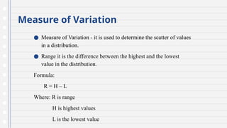
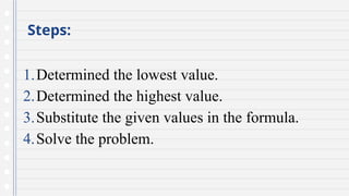
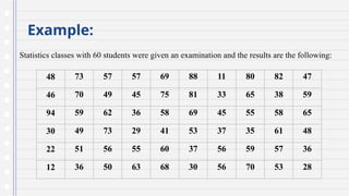
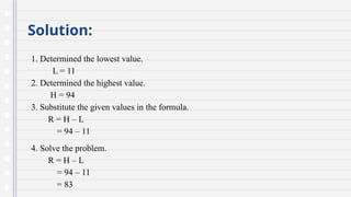
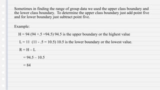
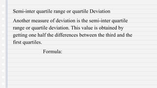
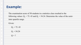
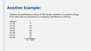
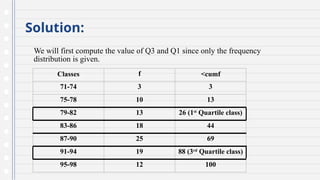
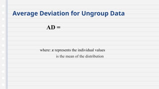
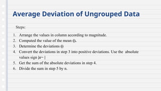
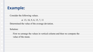
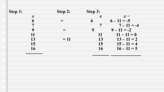
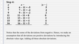
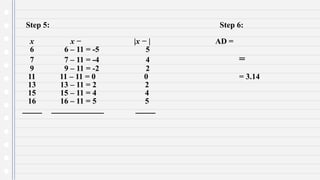
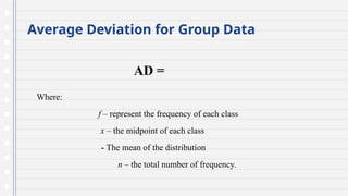
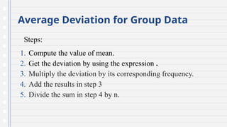
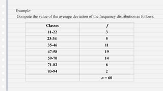
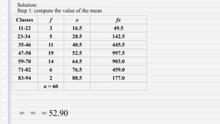
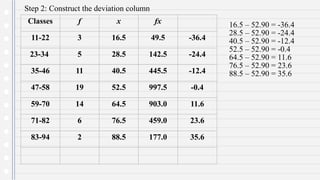
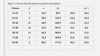
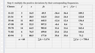
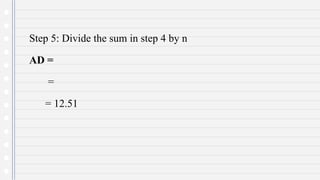
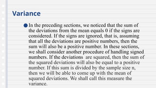
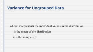
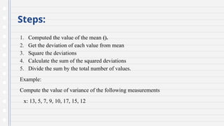
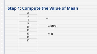
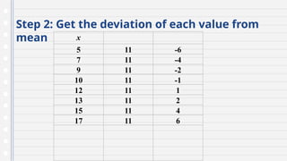
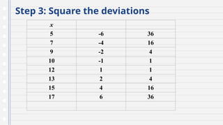
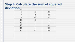
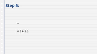
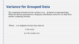
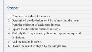
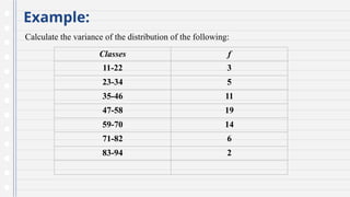
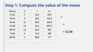
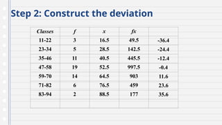
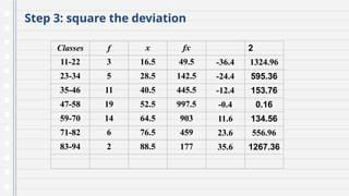
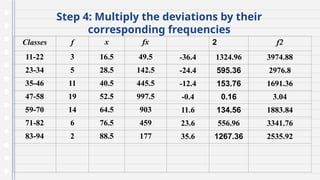
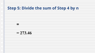
Measure of Variation
● Measure of Variation - it is used to determine the scatter of values
in a distribution.
● Range it is the difference between the highest and the lowest
value in the distribution.
Formula:
R = H – L
Where: R is range
H is highest values
L is the lowest value
Steps:
1.Determined the lowest value.
2.Determined the highest value.
3.Substitute the given values in the formula.
4.Solve the problem.
Example:
Statistics classes with 60 students were given an examination and the results are the following:
48 73 57 57 69 88 11 80 82 47
46 70 49 45 75 81 33 65 38 59
94 59 62 36 58 69 45 55 58 65
30 49 73 29 41 53 37 35 61 48
22 51 56 55 60 37 56 59 57 36
12 36 50 63 68 30 56 70 53 28
Solution:
1. Determined the lowest value.
L = 11
2. Determined the highest value.
H = 94
3. Substitute the given values in the formula.
R = H – L
= 94 – 11
4. Solve the problem.
R = H – L
= 94 – 11
= 83
Sometimes in finding the range of group data we used the upper class boundary and
the lower class boundary. To determine the upper class boundary just add point five
and for lower boundary just subtract point five.
Example:
H = 94 (94 +.5 =94.5) 94.5 is the upper boundary or the highest value
L = 11 (11 - .5 = 10.5) 10.5 is the lower boundary or the lowest value.
R = H – L
= 94.5 – 10.5
= 84
Semi-inter quartile range or quartile Deviation
Another measure of deviation is the semi-inter quartile
range or quartile deviation. This value is obtained by
getting one half the differences between the third and the
first quartiles.
Formula:
Example:
The examination score of 50 students in a statistics class resulted to the
following values: Q3 = 75. 43 and Q1 = 54.24. Determine the value of the semi-
inter quartile range.
Given:
Q3 = 75. 43
Q1 = 54.24
Q = ?
Solution:
Another Example:
Suppose the performance rating of 100 faculty members of a certain college
were taken and are presented in a frequency distribution as follows:
Classes f
71-74 3
75-78 10
79-82 13
83-86 18
87-90 25
91-94 19
95-98 12
n = 100
Solution:
We will first compute the value of Q3 and Q1 since only the frequency
distribution is given.
Classes f <cumf
71-74 3 3
75-78 10 13
79-82 13 26 (1st
Quartile class)
83-86 18 44
87-90 25 69
91-94 19 88 (3rd
Quartile class)
95-98 12 100
Formula:
Solution:
Formula:
Solution:
The value of Q can now be obtained. Thus,
Average
Deviation
●The average deviation refers to the
arithmetic mean of the absolute deviations
of the values from the mean of the
distribution. This measure in sometimes
referred to as the mean absolute deviation.
Average Deviation for Ungroup Data
AD =
where: x represents the individual values
is the mean of the distribution
Average Deviation of Ungrouped Data
Steps:
1. Arrange the values in column according to magnitude.
2. Computed the value of the mean ().
3. Determine the deviations ()
4. Convert the deviations in step 3 into positive deviations. Use the absolute
values sign |x− |
5. Get the sum of the absolute deviations in step 4.
6. Divide the sum in step 5 by n.
Example:
Consider the following values.
x: 13, 16, 9, 6, 15, 7, 11
Determined the value of the average deviation.
Solution:
First we arrange the values in vertical column and then we compute the
value of the mean.
Step 1: Step 2: Step 3:
x x x −
6 = 6 6 – 11 = -5
7 7 7 – 11 = -4
9 = 9 9 – 11 = -2
11 11 11 – 11 = 0
13 = 11 13 13 – 11 = 2
15 15 15 – 11 = 4
16 16 16 – 11 = 5
Step 4:
x x − |x − |
6 6 – 11 = -5 5
7 7 – 11 = -4 4
9 9 – 11 = -2 2
11 11 – 11 = 0 0
13 13 – 11 = 2 2
15 15 – 11 = 4 4
16 16 – 11 = 5 5
Notice that the some of the deviations from negative. Hence, we make an
assumption that all deviations are positive deviations by introducing the
absolute value sign. Adding all these absolute deviations.
Step 5: Step 6:
x x − |x − | AD =
6 6 – 11 = -5 5
7 7 – 11 = -4 4 =
9 9 – 11 = -2 2
11 11 – 11 = 0 0 = 3.14
13 13 – 11 = 2 2
15 15 – 11 = 4 4
16 16 – 11 = 5 5
Average Deviation for Group Data
AD =
Where:
f – represent the frequency of each class
x – the midpoint of each class
- The mean of the distribution
n – the total number of frequency.
Average Deviation for Group Data
Steps:
1. Compute the value of mean.
2. Get the deviation by using the expression .
3. Multiply the deviation by its corresponding frequency.
4. Add the results in step 3
5. Divide the sum in step 4 by n.
Example:
Compute the value of the average deviation of the frequency distribution as follows:
Classes f
11-22 3
23-34 5
35-46 11
47-58 19
59-70 14
71-82 6
83-94 2
n = 60
Solution:
Step 1: compute the value of the mean
= = = 52.90
Classes f x fx
11-22 3 16.5 49.5
23-34 5 28.5 142.5
35-46 11 40.5 445.5
47-58 19 52.5 997.5
59-70 14 64.5 903.0
71-82 6 76.5 459.0
83-94 2 88.5 177.0
n = 60
Step 2: Construct the deviation column
16.5 – 52.90 = -36.4
28.5 – 52.90 = -24.4
40.5 – 52.90 = -12.4
52.5 – 52.90 = -0.4
64.5 – 52.90 = 11.6
76.5 – 52.90 = 23.6
88.5 – 52.90 = 35.6
Classes f x fx
11-22 3 16.5 49.5 -36.4
23-34 5 28.5 142.5 -24.4
35-46 11 40.5 445.5 -12.4
47-58 19 52.5 997.5 -0.4
59-70 14 64.5 903.0 11.6
71-82 6 76.5 459.0 23.6
83-94 2 88.5 177.0 35.6
Step 3: Convert the deviations to positive deviations
Classes f x fx |x− |
11-22 3 16.5 49.5 -36.4 36.4
23-34 5 28.5 142.5 -24.4 24.4
35-46 11 40.5 445.5 -12.4 12.4
47-58 19 52.5 997.5 -0.4 0.4
59-70 14 64.5 903.0 11.6 11.6
71-82 6 76.5 459.0 23.6 23.6
83-94 2 88.5 177.0 35.6 35.6
Step 4: multiply the positive deviations by their corresponding frequencies.
Classes f x fx |x− | f |x− |
11-22 3 16.5 49.5 -36.4 36.4 109.2
23-34 5 28.5 142.5 -24.4 24.4 122.0
35-46 11 40.5 445.5 -12.4 12.4 136.4
47-58 19 52.5 997.5 -0.4 0.4 7.6
59-70 14 64.5 903.0 11.6 11.6 162.4
71-82 6 76.5 459.0 23.6 23.6 141.6
83-94 2 88.5 177.0 35.6 35.6 71.2
n = 60 ∑fx = 3,174 ∑f |x− | = 750.4
Step 5: Divide the sum in step 4 by n
AD =
=
= 12.51
Variance
●In the preceding sections, we noticed that the sum of
the deviations from the mean equals 0 if the signs are
considered. If the signs are ignored, that is, assuming
that all the deviations are positive numbers, then the
sum will also be a positive number. In these sections,
we shall consider another procedure of handling signed
numbers. If the deviations are squared, then the sum of
the squared deviations will also be equal to a positive
number. If this sum is divided by the sample size n,
then we will be able to come up with the mean of
squared deviations. We shall call this measure the
variance.
Variance for Ungrouped Data
where: x represents the individual values in the distribution
is the mean of the distribution
n is the sample size
Steps:
1. Computed the value of the mean ().
2. Get the deviation of each value from mean
3. Square the deviations
4. Calculate the sum of the squared deviations
5. Divide the sum by the total number of values.
Example:
Compute the value of variance of the following measurements
x: 13, 5, 7, 9, 10, 17, 15, 12
Step 1: Compute the Value of Mean
x
5
7
9
10
12
13
15
17
=
= 88/8
= 11
Step 2: Get the deviation of each value from
mean x
5 11 -6
7 11 -4
9 11 -2
10 11 -1
12 11 1
13 11 2
15 11 4
17 11 6
Step 3: Square the deviations
x
5 -6 36
7 -4 16
9 -2 4
10 -1 1
12 1 1
13 2 4
15 4 16
17 6 36
Step 4: Calculate the sum of squared
deviation x
5 -6 36
7 -4 16
9 -2 4
10 -1 1
12 1 1
13 2 4
15 4 16
17 6 36
Step 5:
=
= 14.25
Variance for Grouped Data
The computing formulas for the variance as in is based on ungrouped data.
When the data are presented in a frequency distribution, however, we shall have
another computing formula.
Where: x is midpoint of each class interval
is the mean
n is the sample size
Steps:
1. Compute the value of the mean.
2. Determined the deviation x− by subtracting
x
̄ the mean
from the midpoint of each class interval.
3. Square the deviations obtained in step 2.
4. Multiply the frequencies by their corresponding squared
deviations.
5. Add the results in step 4.
6. Divide the result in step 5 by the sample size.
Example:
Calculate the variance of the distribution of the following:
Classes f
11-22 3
23-34 5
35-46 11
47-58 19
59-70 14
71-82 6
83-94 2
Step 1: Compute the value of the mean
Classes f x fx
11-22 3 16.5 49.5
23-34 5 28.5 142.5
35-46 11 40.5 445.5
47-58 19 52.5 997.5
59-70 14 64.5 903
71-82 6 76.5 459
83-94 2 88.5 177
=
=
= 52.90
Step 2: Construct the deviation
Classes f x fx
11-22 3 16.5 49.5 -36.4
23-34 5 28.5 142.5 -24.4
35-46 11 40.5 445.5 -12.4
47-58 19 52.5 997.5 -0.4
59-70 14 64.5 903 11.6
71-82 6 76.5 459 23.6
83-94 2 88.5 177 35.6
Step 3: square the deviation
Classes f x fx 2
11-22 3 16.5 49.5 -36.4 1324.96
23-34 5 28.5 142.5 -24.4 595.36
35-46 11 40.5 445.5 -12.4 153.76
47-58 19 52.5 997.5 -0.4 0.16
59-70 14 64.5 903 11.6 134.56
71-82 6 76.5 459 23.6 556.96
83-94 2 88.5 177 35.6 1267.36
Step 4: Multiply the deviations by their
corresponding frequencies
Classes f x fx 2 f2
11-22 3 16.5 49.5 -36.4 1324.96 3974.88
23-34 5 28.5 142.5 -24.4 595.36 2976.8
35-46 11 40.5 445.5 -12.4 153.76 1691.36
47-58 19 52.5 997.5 -0.4 0.16 3.04
59-70 14 64.5 903 11.6 134.56 1883.84
71-82 6 76.5 459 23.6 556.96 3341.76
83-94 2 88.5 177 35.6 1267.36 2535.92
Step 5: Divide the sum of Step 4 by n
=
= 273.46
Chapter-6-Variance Purposive Communication.pptx

Chapter-6-Variance Purposive Communication.pptx

  • 1.
    Measure of Variation ●Measure of Variation - it is used to determine the scatter of values in a distribution. ● Range it is the difference between the highest and the lowest value in the distribution. Formula: R = H – L Where: R is range H is highest values L is the lowest value
  • 2.
    Steps: 1.Determined the lowestvalue. 2.Determined the highest value. 3.Substitute the given values in the formula. 4.Solve the problem.
  • 3.
    Example: Statistics classes with60 students were given an examination and the results are the following: 48 73 57 57 69 88 11 80 82 47 46 70 49 45 75 81 33 65 38 59 94 59 62 36 58 69 45 55 58 65 30 49 73 29 41 53 37 35 61 48 22 51 56 55 60 37 56 59 57 36 12 36 50 63 68 30 56 70 53 28
  • 4.
    Solution: 1. Determined thelowest value. L = 11 2. Determined the highest value. H = 94 3. Substitute the given values in the formula. R = H – L = 94 – 11 4. Solve the problem. R = H – L = 94 – 11 = 83
  • 5.
    Sometimes in findingthe range of group data we used the upper class boundary and the lower class boundary. To determine the upper class boundary just add point five and for lower boundary just subtract point five. Example: H = 94 (94 +.5 =94.5) 94.5 is the upper boundary or the highest value L = 11 (11 - .5 = 10.5) 10.5 is the lower boundary or the lowest value. R = H – L = 94.5 – 10.5 = 84
  • 6.
    Semi-inter quartile rangeor quartile Deviation Another measure of deviation is the semi-inter quartile range or quartile deviation. This value is obtained by getting one half the differences between the third and the first quartiles. Formula:
  • 7.
    Example: The examination scoreof 50 students in a statistics class resulted to the following values: Q3 = 75. 43 and Q1 = 54.24. Determine the value of the semi- inter quartile range. Given: Q3 = 75. 43 Q1 = 54.24 Q = ?
  • 8.
  • 9.
    Another Example: Suppose theperformance rating of 100 faculty members of a certain college were taken and are presented in a frequency distribution as follows: Classes f 71-74 3 75-78 10 79-82 13 83-86 18 87-90 25 91-94 19 95-98 12 n = 100
  • 10.
    Solution: We will firstcompute the value of Q3 and Q1 since only the frequency distribution is given. Classes f <cumf 71-74 3 3 75-78 10 13 79-82 13 26 (1st Quartile class) 83-86 18 44 87-90 25 69 91-94 19 88 (3rd Quartile class) 95-98 12 100
  • 11.
  • 12.
    The value ofQ can now be obtained. Thus,
  • 13.
    Average Deviation ●The average deviationrefers to the arithmetic mean of the absolute deviations of the values from the mean of the distribution. This measure in sometimes referred to as the mean absolute deviation.
  • 14.
    Average Deviation forUngroup Data AD = where: x represents the individual values is the mean of the distribution
  • 15.
    Average Deviation ofUngrouped Data Steps: 1. Arrange the values in column according to magnitude. 2. Computed the value of the mean (). 3. Determine the deviations () 4. Convert the deviations in step 3 into positive deviations. Use the absolute values sign |x− | 5. Get the sum of the absolute deviations in step 4. 6. Divide the sum in step 5 by n.
  • 16.
    Example: Consider the followingvalues. x: 13, 16, 9, 6, 15, 7, 11 Determined the value of the average deviation. Solution: First we arrange the values in vertical column and then we compute the value of the mean.
  • 17.
    Step 1: Step2: Step 3: x x x − 6 = 6 6 – 11 = -5 7 7 7 – 11 = -4 9 = 9 9 – 11 = -2 11 11 11 – 11 = 0 13 = 11 13 13 – 11 = 2 15 15 15 – 11 = 4 16 16 16 – 11 = 5
  • 18.
    Step 4: x x− |x − | 6 6 – 11 = -5 5 7 7 – 11 = -4 4 9 9 – 11 = -2 2 11 11 – 11 = 0 0 13 13 – 11 = 2 2 15 15 – 11 = 4 4 16 16 – 11 = 5 5 Notice that the some of the deviations from negative. Hence, we make an assumption that all deviations are positive deviations by introducing the absolute value sign. Adding all these absolute deviations.
  • 19.
    Step 5: Step6: x x − |x − | AD = 6 6 – 11 = -5 5 7 7 – 11 = -4 4 = 9 9 – 11 = -2 2 11 11 – 11 = 0 0 = 3.14 13 13 – 11 = 2 2 15 15 – 11 = 4 4 16 16 – 11 = 5 5
  • 20.
    Average Deviation forGroup Data AD = Where: f – represent the frequency of each class x – the midpoint of each class - The mean of the distribution n – the total number of frequency.
  • 21.
    Average Deviation forGroup Data Steps: 1. Compute the value of mean. 2. Get the deviation by using the expression . 3. Multiply the deviation by its corresponding frequency. 4. Add the results in step 3 5. Divide the sum in step 4 by n.
  • 22.
    Example: Compute the valueof the average deviation of the frequency distribution as follows: Classes f 11-22 3 23-34 5 35-46 11 47-58 19 59-70 14 71-82 6 83-94 2 n = 60
  • 23.
    Solution: Step 1: computethe value of the mean = = = 52.90 Classes f x fx 11-22 3 16.5 49.5 23-34 5 28.5 142.5 35-46 11 40.5 445.5 47-58 19 52.5 997.5 59-70 14 64.5 903.0 71-82 6 76.5 459.0 83-94 2 88.5 177.0 n = 60
  • 24.
    Step 2: Constructthe deviation column 16.5 – 52.90 = -36.4 28.5 – 52.90 = -24.4 40.5 – 52.90 = -12.4 52.5 – 52.90 = -0.4 64.5 – 52.90 = 11.6 76.5 – 52.90 = 23.6 88.5 – 52.90 = 35.6 Classes f x fx 11-22 3 16.5 49.5 -36.4 23-34 5 28.5 142.5 -24.4 35-46 11 40.5 445.5 -12.4 47-58 19 52.5 997.5 -0.4 59-70 14 64.5 903.0 11.6 71-82 6 76.5 459.0 23.6 83-94 2 88.5 177.0 35.6
  • 25.
    Step 3: Convertthe deviations to positive deviations Classes f x fx |x− | 11-22 3 16.5 49.5 -36.4 36.4 23-34 5 28.5 142.5 -24.4 24.4 35-46 11 40.5 445.5 -12.4 12.4 47-58 19 52.5 997.5 -0.4 0.4 59-70 14 64.5 903.0 11.6 11.6 71-82 6 76.5 459.0 23.6 23.6 83-94 2 88.5 177.0 35.6 35.6
  • 26.
    Step 4: multiplythe positive deviations by their corresponding frequencies. Classes f x fx |x− | f |x− | 11-22 3 16.5 49.5 -36.4 36.4 109.2 23-34 5 28.5 142.5 -24.4 24.4 122.0 35-46 11 40.5 445.5 -12.4 12.4 136.4 47-58 19 52.5 997.5 -0.4 0.4 7.6 59-70 14 64.5 903.0 11.6 11.6 162.4 71-82 6 76.5 459.0 23.6 23.6 141.6 83-94 2 88.5 177.0 35.6 35.6 71.2 n = 60 ∑fx = 3,174 ∑f |x− | = 750.4
  • 27.
    Step 5: Dividethe sum in step 4 by n AD = = = 12.51
  • 28.
    Variance ●In the precedingsections, we noticed that the sum of the deviations from the mean equals 0 if the signs are considered. If the signs are ignored, that is, assuming that all the deviations are positive numbers, then the sum will also be a positive number. In these sections, we shall consider another procedure of handling signed numbers. If the deviations are squared, then the sum of the squared deviations will also be equal to a positive number. If this sum is divided by the sample size n, then we will be able to come up with the mean of squared deviations. We shall call this measure the variance.
  • 29.
    Variance for UngroupedData where: x represents the individual values in the distribution is the mean of the distribution n is the sample size
  • 30.
    Steps: 1. Computed thevalue of the mean (). 2. Get the deviation of each value from mean 3. Square the deviations 4. Calculate the sum of the squared deviations 5. Divide the sum by the total number of values. Example: Compute the value of variance of the following measurements x: 13, 5, 7, 9, 10, 17, 15, 12
  • 31.
    Step 1: Computethe Value of Mean x 5 7 9 10 12 13 15 17 = = 88/8 = 11
  • 32.
    Step 2: Getthe deviation of each value from mean x 5 11 -6 7 11 -4 9 11 -2 10 11 -1 12 11 1 13 11 2 15 11 4 17 11 6
  • 33.
    Step 3: Squarethe deviations x 5 -6 36 7 -4 16 9 -2 4 10 -1 1 12 1 1 13 2 4 15 4 16 17 6 36
  • 34.
    Step 4: Calculatethe sum of squared deviation x 5 -6 36 7 -4 16 9 -2 4 10 -1 1 12 1 1 13 2 4 15 4 16 17 6 36
  • 35.
  • 36.
    Variance for GroupedData The computing formulas for the variance as in is based on ungrouped data. When the data are presented in a frequency distribution, however, we shall have another computing formula. Where: x is midpoint of each class interval is the mean n is the sample size
  • 37.
    Steps: 1. Compute thevalue of the mean. 2. Determined the deviation x− by subtracting x ̄ the mean from the midpoint of each class interval. 3. Square the deviations obtained in step 2. 4. Multiply the frequencies by their corresponding squared deviations. 5. Add the results in step 4. 6. Divide the result in step 5 by the sample size.
  • 38.
    Example: Calculate the varianceof the distribution of the following: Classes f 11-22 3 23-34 5 35-46 11 47-58 19 59-70 14 71-82 6 83-94 2
  • 39.
    Step 1: Computethe value of the mean Classes f x fx 11-22 3 16.5 49.5 23-34 5 28.5 142.5 35-46 11 40.5 445.5 47-58 19 52.5 997.5 59-70 14 64.5 903 71-82 6 76.5 459 83-94 2 88.5 177 = = = 52.90
  • 40.
    Step 2: Constructthe deviation Classes f x fx 11-22 3 16.5 49.5 -36.4 23-34 5 28.5 142.5 -24.4 35-46 11 40.5 445.5 -12.4 47-58 19 52.5 997.5 -0.4 59-70 14 64.5 903 11.6 71-82 6 76.5 459 23.6 83-94 2 88.5 177 35.6
  • 41.
    Step 3: squarethe deviation Classes f x fx 2 11-22 3 16.5 49.5 -36.4 1324.96 23-34 5 28.5 142.5 -24.4 595.36 35-46 11 40.5 445.5 -12.4 153.76 47-58 19 52.5 997.5 -0.4 0.16 59-70 14 64.5 903 11.6 134.56 71-82 6 76.5 459 23.6 556.96 83-94 2 88.5 177 35.6 1267.36
  • 42.
    Step 4: Multiplythe deviations by their corresponding frequencies Classes f x fx 2 f2 11-22 3 16.5 49.5 -36.4 1324.96 3974.88 23-34 5 28.5 142.5 -24.4 595.36 2976.8 35-46 11 40.5 445.5 -12.4 153.76 1691.36 47-58 19 52.5 997.5 -0.4 0.16 3.04 59-70 14 64.5 903 11.6 134.56 1883.84 71-82 6 76.5 459 23.6 556.96 3341.76 83-94 2 88.5 177 35.6 1267.36 2535.92
  • 43.
    Step 5: Dividethe sum of Step 4 by n = = 273.46