SlideShare a Scribd company logo
1 of 43
Download to read offline
1	
	
Belarusian Economic Research and Outreach Center
Working Paper Series
BEROC WP No. 47
Determinants of poverty with and without economic growth. Explaining Belarus's poverty
dynamics during 2009-2016.
Aleh Mazol
November 2017
Abstract
This paper studies the incidence and determinants of poverty in Belarus using data from yearly
Household Budget Surveys for 2009-2016. The poverty is evaluated from consumption perspective
applying the cost of basic needs approach and using food and absolute poverty lines. During last
two years, absolute poverty in Belarus has increased twofold and reached 29% of the population.
Household size, number of children, lonely mothers and labor status of the household members are
among the key determinants of household welfare and poverty. Moreover, living in rural areas and in
Brest, Gomel and Mogilev regions increases the likelihood of being poor and negatively relates with
welfare. Therefore, public policy directed towards the provision of better family planning, education
as well as more diverse possibilities for financial investment, labor market reform targeted for
productive job creation, increased non-agricultural employment opportunities for rural residents and
additional location specific efforts in Brest, Gomel and Mogilev regions should be among the
strategies for poverty reduction in Belarus.
Keywords: poverty, income, consumption, household, survey, Belarus
JEL Classification: E20, I32, O18, R23
Belarusian Economic Research and Outreach Center (BEROC) started its work as joint project of
Stockholm Institute of Transition Economics (SITE) and Economics Education and Research
Consortium (EERC) in 2008 with financial support from SIDA and USAID. The mission of
BEROC is to spread the international academic standards and values through academic and policy
research, modern economic education and strengthening of communication and networking with
the world academic community.
2	
	
1. Introduction
Poverty reduction and general wellbeing are public policy goals commonly pursued by the Belarusian
government today. Since 2000, Belarus's economic growth not only has noticeably enhanced the
average standard of living in Belarus, but also has raised substantial number of Belarusians out of
poverty. According to official estimates, the poverty rate in Belarus has decreased from 41.9% of the
population in 2000 up to 5.2% in 2010 and currently hovers around 6% (during 2011-2016).1
This
was a remarkable result achieved in a very short period.2
However, economic downturns may introduce considerable survival problems for many households.
For example, according to the World Bank, in some countries the poverty rate may reach 50%
because of an economic crisis (World Bank, 2000a; 2005).3
In this regard, small increase in the
official poverty during periods of economic crises in the country (2009, 2011 and 2015-2016) casts
doubt on Belarus's record in poverty reduction.
Moreover, both the construction and the assessment of the anti-poverty policies are dependent on
precise appraisal of the actual degree of poverty. Even an estimated error of only a few percentage
points would have notable consequences: hundreds of thousands of people in Belarus would be
wrongly classified as non-poor, weakening the government's anti-poverty policy.
In this regard, the official methodology to measure poverty4
(uses the definition of family income –
disposable income, that is compared to poverty threshold – national poverty line) suffers from
several drawbacks.
First, largest share (over 60%) of calories in the budget of the subsistence minimum (MSB) used to
define poverty threshold in Belarus comes from rye bread, cereals, milk, dairy products, eggs and fat
that are the cheapest source of calories. Therefore, it would be relatively easy to construct a poverty
line that satisfies a minimum caloric requirement and is consistent with comparatively low level of
household income, thus achieving low incidence of poverty in Belarus.
Second, the share of cost of non-food items in the MSB should be estimated at the level of total
food cost of households around the food poverty line (i.e. low-income families), in comparison with
current more austere definition of using total cost. Poverty levels and changes are clearly sensitive to
																																																													
1 Belstat.
2 The largest reported decline in poverty was in 2001, from 41.9% in 2000 to 28.9% occurred on the background of a
relatively modest yearly growth performance (4.7% of GDP).
3 The main paths for transmission of the adverse effects to the economy were reductions in social spending and
government transfers, the impairment of savings affected by hyperinflation and subsequent devaluation of the national
currency, and overall corrections to the labor market (World Bank, 2000a; 2005).
4 Official poverty measurement is based on comparison of per capita disposable income of household with national
poverty line, which is the average per capita budget of the subsistence minimum (MSB) of a family of four containing
two adults and two children. The MSB is a minimum set of goods and services needed to guarantee the sustainability of
the family, preservation of health of its members, as well as compulsory payments and contributions. The MSB of a
family of four is based on 42 food items and hundreds of other non-food items categorized under the following
categories: clothing and footwear; home amenities; sanitary, hygiene and medical products; housing; and
communications and services. The cost of non-food goods and services is defined as a fixed share of 77% of the cost of
the food goods. The MSB is calculated on a quarterly basis by the Ministry of Labor and Social Protection of the
Republic of Belarus in the prices of the last month of the quarter.
3	
	
where the poverty line is set (i.e. the higher is the share of non-food goods, the higher is the poverty
threshold).
Third, poverty threshold is not adjusted for geographic differences in the cost of living, since the
official poverty measurement does not consider regional variations in calorie diet and also does not
take into account regional differences in food and non-food prices. Official price index, such as CPI,
reflect the increase in cost of living for an average household.
Fourth, using an income measure for assessing poverty is problematic due to a controlled income
policy in Belarus including administrative wage increases and subsequent corrections in pensions.
Wages and pensions account for approximately three quarters of disposable income of households
in Belarus.
Fifth, another odd consequence of applying income aggregate would be to place wrongly younger
households above the poverty line. For example, young renters who have above average incomes,
but pay a substantial proportion of what they do earn in rent are one such group. Moreover, income
is sensitive to volatile shocks and with the possibility of households to smooth their consumption
through time using borrowings, savings, and mutual insurance, consumption measures are
considered much more reliable and more theoretically sound (Ravallion, 1996; Deaton, 1997).
Finally, the inconsistency in the official poverty measurement in Belarus can be attributed also to
constant changes in the national poverty line over time due to normative considerations. For
example, before 2014 the cost of non-food items in the MSB was calculated using predefined
norms, while after – as a share.
Therefore, the main goal of the research is to determine and measure poverty in Belarus more
accurately in order to present improved evidence for public policy intervention. Correspondingly,
this paper has several broad objectives. First, to provide a descriptive characterization of poverty in
Belarus by undertaking a detailed analysis of the factors influencing welfare and poverty at the
household level; and by determining which regions and areas of Belarus have highest levels of
poverty. Second, it aims to contribute to the literature of poverty studies. To date, there has been
very little analysis of poverty dynamics in Belarus – for example, studies that examine the welfare
movements of households over time. Third, this paper is the first study that tries to shed light how
financial and economic downturns happened in 2011 and 2015-2016 in Belarus adjusted poverty
status of households in Belarus.
The paper uses data from yearly Household Budget Surveys in Belarus for 2009-2016 and applies a
poverty measurement methodology based on food and absolute poverty lines skipping issues related
to capabilities, social exclusion and participation (Laderchi et al., 2003) and constructing a household
welfare aggregate comparable over time and across different regions of Belarus. In particular, the
welfare measure is based on household consumption, deflated to take into account differences in
purchasing power over time and regions of residence and corrected per person nutrition
requirements among households of different size and demographic composition.
4	
	
Next, in order to identify food and absolute poverty lines in Belarus the cost of basic needs
approach is used.5
This method stipulates a minimum consumer basket (including food and non-
food items) adequate for basic consumption needs. In this way, the research adopts the approach of
previous studies of poverty dynamics and follow next microeconomic assumptions: first, human
behavior follows utility maximization model; second, expenditures display the marginal value people
place on goods; and, third, expenditure data can be considered as a proxy for consumption as a
welfare measure (Laderchi et al., 2003).
Finally, the paper emphasizes on several common associations of poverty found both for developing
and transition countries. For instance, the poverty is typically higher in households with single
parent, in households where the number of dependants related to income earners is on average
higher, and in large households (Milanovic, 1996; Lokshin & Popkin, 1999). Additionally, other
factors that usually define poverty in less developed countries including the evidence of higher
poverty for the elderly in the region (Milanovic, 1996; Klugman et al., 2002), the evidence that
households with low educated heads or main income earners were most probably to be in poverty
(World Bank, 2000a, 2005), the influence of unemployment (World Bank, 2000a, 2005) will also be
studied.
The empirical strategy of the research consists of the following steps and methods: (1) setting the
food and absolute poverty lines using the cost of basic needs approach; (2) estimating poverty
measures based on Foster-Greer-Thorbecke's poverty indices; (3) analyzing the determinants of
welfare and poverty using OLS and probit regressions.
The main results of the research are:
§ During 2009-2011, poverty at the national level stayed almost unchanged reaching 32.6% of
the population. During 2012-2014 there was a substantial decrease in incidence of poverty (by
18 percentage points) caused mostly by the strong growth of household incomes (by 39%). In
contrast, economic crisis in 2015-2016 was associated with a twofold increase in incidence,
depth and severity of poverty in Belarus.
§ The analysis also shows that considerably more poverty exists in the rural areas of Belarus
than in urban areas. A poverty incidence for the nation's rural areas over 2009-2016 is
approximately 10.5 percentage points (or 44%) higher than the national average, while that of
the urban areas is nearly 4 percentage points (or 16%) below national average.
§ The results indicate presence of large regional differences in poverty. In particular, a poverty
incidence for Grodno region in 2016 is roughly 3% below the national average, that for the
Brest and Mogilev regions are 31% and 21% higher than this average, correspondingly.
§ Among factors that substantially decrease household welfare and increase poverty at the
household level in Belarus are family size, the number of children in a household, presence in
																																																													
5 Unlike the official methodology the cost of basic needs approach meets the following four requirements: (1)
conformity with national recommendations for minimum nutritional intakes; (2) tailoring to family size and both gender
and age calorie needs; and (3) reflection of market prices with poverty lines adjusted to take into account price
differentials into account.
5	
	
the household of economically inactive members. Moreover, lonely mothers in Belarus appear
to be noticeably more vulnerable to macroeconomic shocks than full families both from
welfare and poverty perspectives. Additionally, one of the most important determinants of
welfare and poverty in all samples is spatial location of household. Poverty highly
discriminates against living in rural areas, Brest, Gomel and Mogilev regions.
§ Finally, on average, large positive influence on consumption expenditure and negative on the
chance of getting poor have savings and access to landplot.
The rest of the paper is structured as follows. Section 2 presents the literature review. Section 3
describes the methodology used in the research and guides the empirical analysis. Section 4 discusses
the data used. Section 5 presents and interprets the results of the analysis. Finally, Section 6
concludes and develops some implications for public policy intervention.
2. Literature Review
2.1. Theory
Poverty by itself means the absence of an acceptable minimum level of material welfare. There are
four main objectives to measure poverty (Srinivasan, 2001). First, its assessment is necessary to
describe the extent of poverty in a particular point of time or geographical location for
governmental accountability and monitoring the fulfillment of public programmes. Second,
measurement is required to study the determinants of poverty. Third, in order to develop an
effective poverty-alleviating strategy in the country the correct identification of the socio-economic
characteristics of individuals and households that move in and out of poverty is crucial. Finally,
these characteristics play a significant role in the understanding of the influence of economic crises
on households, which will help to develop better policies that would protect their welfare (Dollar &
Kraay, 2002; Ravallion, 2001; Ravallion, 2005).
Correspondingly, in the last case poverty becomes one of the defining issues for the state, because
economic downturns may introduce substantial survival problems for many households. For
example, according to the World Bank, in some countries the poverty rate may reach 50% because
of an economic crisis (World Bank, 2000a; 2005). Consequently, the investigation of determinants
and dynamics of poverty has received additional attention in studies concerning developing
economies that constantly suffer from economic and financial shocks (e.g. Bane & Ellwood, 1986;
Layte & Whelan, 2003).
The key effects of economic downturns on households contain increase in unemployment, cuts in
social spending and public transfers, loss of financial savings because of rising inflation and a sharp
devaluation of the national currency due to financial instability that often accompanies or precedes
economic crises. As a result, the labor market adjusts to falling demand for labor, caused, first, by
the decline in production, and, second, as a consequence of the inefficient use of labor resources in
previous years (Adam, 1982). These adjustments to labor market happen through a decline in real
wages, a fall in employment and rise in unemployment. Moreover, these changes are accompanied
6	
	
by the sectoral and occupational reallocation of labor jointly with the additional corrections in the
relative level of wages (Jackman, 1998), which subsequently causes drop in households'
consumption.
In addition to above direct effects of the economic fluctuations on households, there are also
indirect effects originating from the financial instability that by itself generates growth instability.
This situation occurs because financial shocks destabilize investments (the level of investment
depends on the availability of finance) and, consequently, the rate of economic growth. Moreover,
financial instability leads to a volatility of relative prices since the prices of different goods or
services are not influenced in the same proportion: prices of tradable goods are determined by
foreign prices and the nominal exchange rate, while prices of non-tradable goods are subject to the
domestic supply and demand. Both the instability of investment and the real exchange rate lead to
growth volatility, which may increase or prolong corrections to welfare of households.
Moreover, due to asymmetry between periods of decreasing and rising of aggregate income, caused
by periods of expansion and contraction in the economy, poor households may be more exposed to
cyclical fluctuations of economic growth than the rich ones (de Janvry & Sadoulet, 2000). This
asymmetry is possibly the result of several factors that can vary from one country to another. From
one hand, the less skilled and poorest workers lose their jobs first and when the expansions starts
they were unemployed for a longer period. This is so-called the effect of delay, when the former
unemployed are the last to be hired. Second, since prices rarely decrease during recessions, they
most common increase during expansions. The poor households are supposed to depend more on
state determined income (such as pension, state subsidies or direct transfers) than the rich ones,
which is only party corrected for inflation (Easterly & Fischer, 2001).
Furthermore, the poverty is mostly concentrated in rural areas. Governments generally do not
correct for growth of international prices for exports of agricultural products for the rural
households, while they pass the price drop on them due to budget constraints. As a result, since they
receive no benefit from the insurance scheme, the decrease in the incomes of poor people can lead
them to worry less about their health, the education of their children, which in the long-run harms
their human capital and overall human development of the country.
Therefore, the above issues rise questions of how household may cope with economic crises.
According to one strand of literature, namely the life-cycle theory, households use wealth
accumulation to smooth consumption over their life cycle (Ando & Modigliani, 1963). Subsequently,
any unpredicted changes in their wealth, following crisis, may cause households to reconsider their
consumption plans (Modigliani, 1971; Aron et al., 2010; Muellbauer, 2010; Carroll, Otsuka &
Slacalek, 2011), although in the short-run such shocks do not fully pass to consumption.
Households that expect the occurrence of the crisis will tend to smooth consumption and nutrition
plans, which contain spending in the form of livestock and other assets (Dercon, 1996), attempt to
diversify incomes by exploitation of a landplot (Barrett, Reardon & Webb, 2001; Dercon &
Krishnan, 1996).
7	
	
The second direction of economic studies concentrates on precautionary savings and asset levels
investigating the vulnerability of households to economic and financial shocks. In accordance with
this theory, risk-averse individuals facing with the uninsurable risks accumulate wealth to protect
themselves against shocks (Deaton 1992; Carroll, 1997).		However, other empirical studies show that
many households possess few or no assets and no savings and that they are very exposed to shocks
(Caner & Wolff, 2004). Additionally, it was identified the scarcity of assets among certain population
groups (Oliver & Shapiro, 1995; Conley, 1999; Havemann & Wolff, 2004; Bucks, Kennickell &
Moore, 2004; Sherraden, 2005).
Furthermore, households' assets may be scarce not due to their inability to accumulate wealth, but
due to influence of shocks that decrease their savings (Deaton, 1992). Households may rely on their
relatives and friends to deal with unpredicted economic and financial shocks (Briggs, 1998; Sarkasian
& Gerstel, 2004; Henley, Danziger & Offer, 2005; Harknett & Knab, 2007). Finally, other activities
that households can engage when facing shocks may be the increase in their home production of
goods in order to reduce their expenditure (Aguiar & Hurst, 2005). This heterogeneity in behavior of
households may indicate differences in their economic circumstances and opportunity (e.g.,
education), differences in financial capabilities (Lusardi, 2009).
2.2. Empirical research
Past studies in developing countries has shown that households experience poverty caused by
economic downturns differently: richer households are poor for shorter periods of time or
experience one episode of poverty, while poorer families face with long-lasting poverty or have
multiple poverty episodes (Bane & Ellwood, 1986; Gottschalk et al., 1994; Rank & Hirschl, 2001).6
Correspondingly, it was found that periods of recessions decrease the income of the poor greater
than the periods of economic expansions increase. For example, de Janvry and Sadoulet (2000),
studying economic indicators of twelve countries in Latin American countries between 1970 and
1994, have found that economic growth on average has decreased poverty both in urban and rural
areas, but the negative effects of the recessions on poverty was found to be stronger than the
positive effects of economic growth.
Next, existing research has identified several fundamental factors of poverty in developing countries.
For instance, it was considered that the level of poverty is higher among families with many
children, incomplete families and families with a higher than average number of dependents relative
to the number of people receiving income (Milanovic 1996; Lokshin & Popkin, 1999). However, the
evidence of higher poverty risk for the elderly is scarce (Milanovic 1996; Klugman, Micklewright &
Redmond, 2002).
Regarding transition countries, the empirical studies defined that households with low educated
heads or main income providers were more likely to fall into poverty (World Bank, 2005).
Concerning the CIS7
countries this factor showed less relative influence in the 1990s in comparison
																																																													
6 This effect holds also for developed countries.
7 CIS – The Commonwealth of Independent States.
8	
	
with the countries from the Central Europe, but its influence has increased since 2000 (World Bank,
2000a; 2005). Finally, Gustafsson and Nivorozhkina (2004) investigated the evolution of poverty and
its determinants during transition period, but concentrating only on one city. However, generally the
existing studies on the dynamics and determinants of poverty in the CIS countries remain scarce.
The results from studies concerning transition countries that used consumption expenditure and the
basic needs concept showed that 24.5% of Lithuanian population in 2010 was below absolute
poverty line (Sileika, 2011). In Italy the consumption-based measure of absolute poverty was 9.3% in
2013 (Campiglio, 2017). A similar study for Ukraine showed that 23.2% of its population were
consumption poor in 2004 (Bruck et al., 2010); for Russia, Croatia, Hungary, Poland, Latvia,
Azerbaijan, Bulgaria and Slovenia – 14.1%, 12.5%, 17.3%, 10.1%, 12.4%, 78.9%, 67.5% and 3.5%,
correspondingly, in 2010 (Scare & Druzeta, 2014).
Previous empirical studies of poverty in Belarus mostly comes from several reports accomplished by
the World Bank (World Bank, 1996; 2004; Cojocaru & Matytsin, 2017) and by the IPM Research
Center (2017).
Cojocaru and Matytsin (2017) using the international poverty lines (IPL)8
(for example, equaled to
PPP9
10 US Dollar/day threshold) showed that the poverty incidence in Belarus dropped from 82%
in 2003, to less than 10% in 2014, before increasing to 12.3% in 2015 (Cojocaru & Matytsin, 2017).
However, the IPL measures for determining national level of poverty unable to reflect local
circumstances such as spatial price differences and the consumption patterns of the poor, as well as
the country and time-specific composition of households.
Study accomplished by the IPM Research Center showed a static picture based on 2013-2016 yearly
household data. According to their estimates, the rate of absolute poverty in Belarus equaled 4.8%
of the population in 2013 and gradually reached 6.7% in 2016, which is only by one percentage point
higher than the official estimate. However, the IPM Research Center's approach to poverty
estimation in Belarus relied mostly on the same official methodology.10
3. Methodology
There are two main methods in the poverty literature to explain the concept of household welfare:
the monetary and the non-monetary approaches.
The monetary approach to poverty defines welfare in terms of utility (Ravallion, 1994). However,
given that utility cannot be directly estimated, financial resources of a household (expenditure or
income) are used to estimate welfare. These measurements reflect a narrow vision of welfare
																																																													
8 The IPL is used by the World Bank as a common standard for all countries (Ravallion et al., 2008). The basic idea is to
assure that two people who possess the same purchasing power over commodities are classified consistently as either
poor or non-poor regardless of whether they live in same or different countries.
9 PPP – Purchasing Power Parity – the common unit of measurement established by the International Comparison
Programme (ICP) based on collected prices of comparable goods in countries around the world.
10 Modifications: (1) corrections to poverty threshold dependent on age structure of the household; and (2) calculation of
the poverty level accomplished based on annual averages and not on quarterly (IPM Research Center, 2017).
9	
	
(Deaton, 2003), because unable to account for non-quantifiable dimension of household wellbeing,
for example non-market goods and services (Ravallion, 1996).
The non-monetary approach defines, first, the basic needs concept (Asselin & Dauphin, 2001) and,
second, the notion of capability (Sen, 1992). In the first case, poverty is estimated based on the cost
of basic needs (or cost of living for particular household) and using predetermined poverty lines
(Chen & Ravallion, 2004, 2010). The poor are those households, who are deprived of a basic set of
commodities (food, water, health, education, housing, energy etc.), that are essential for obtaining
good standards of living (Asselin & Dauphin, 2001). Therefore, the basic needs concept is less
abstract than pure monetary approach and combines both monetary and non-monetary variables
making it possible to evaluate goods and services directly in terms of human welfare and favors
targeted public policy. The capability approach underlines the concept of "functionings" that takes
into account various things that every individual in the household may value doing or being, such as
being adequately nourished, being healthy, taking part in social life and so on. However, according
to Sen (1992) the set of individual capabilities cannot be directly observed and must be determined
based on presumption. This subjective approach grounds on a value judgment as to what it means
to be poor. It uses data from self-reported assessments of living conditions and determines poverty
using an individual perception of own well-being (see World Bank, 2000; Deaton, 2008).
Hence, in order to take into account the non-monetary aspect of household welfare and to get a
broader view for policy implementation the basic needs approach is used to analyze and measure
poverty in Belarus. This approach estimates poverty using quantifiable dimensions of welfare and
based on objective data provided by each person and/or household in a whole (for example, income
or expenditure).
In this study, consumption expenditure is used to measure welfare. This choice is motivated by
several considerations. First, consumption expenditure shows household's ability to obtain goods
and services. Second, the data collected on consumption are more accurate than the income data
taking into account that people may have reasons to hide part of their earnings (Ravallion, 2001) and
that measured consumption patterns vary less in comparison with estimated income patterns
(Deaton, 1997). For example, an increased income only raises household welfare if it is consumed,
while past income (savings) or borrowings can also be used for consumption purposes. Third,
income is sensitive to volatile shocks and with the possibility of households to smooth their
consumption through time using borrowings, savings, and mutual insurance, consumption measures
are considered much more reliable and more theoretically sound (Ravallion, 1996; Deaton, 1997).
Therefore, consumption expenditure data are supposed to depict household welfare more accurately
in comparison with income, because can be viewed as realized welfare, whereas income is more a
measure of potential welfare.
In the whole, the empirical strategy to evaluate the incidence of poverty among Belarusian
households and its determinants over 2009-2016 involves the following steps and methods: (1)
10	
	
setting the food and absolute poverty lines; (2) estimating poverty measures; (3) analyzing the
determinants of welfare and poverty using OLS and probit regressions.
3.1. Determining the poverty lines
In order to define the poor households in Belarus using the cost of basic needs method two
household-specific poverty lines are estimated: the food poverty line and absolute poverty line (see
Kakwani, 2003). The food poverty line represents the monetary amount needed to cover expenditure on
required calorie intake of a particular household taking into account its age and gender composition
and adjusting for differences in regional food prices (Deaton, 1997; Lanjouw et al., 2004). The
absolute poverty line augments the food poverty line with a non-food allowance. This non-food part is
estimated based on the share of non-food expenditures in total consumption expenditures in a given
year of those households close to the poverty threshold. Thus, the absolute poverty line capture
both food and non-food expenditures and can evaluate poverty more precisely.
Following Ravallion (1994) and Kakwani (2003), the food and absolute poverty lines for each
studied Belarusian household are determined using next five steps:
Step 1: Specifying the calorie requirement. Depending on the age and gender of all household
members from Belarusian Household Budget Surveys for 2009-2016 the required per capita calorie
requirement for each household is defined. For these purposes, the official list of 20 categories of
people (based on age and gender) with different calorie requirements ranging from 110 to 3050 kcal
per person per day is used (see Table A1).
Step 2: Calculating the cost of calories for Belarusian regions. The cost of a calorie separately
for each region of Belarus is determined using the national basic need food basket11
(see Table A2)
and average regional prices12
of each of its items. First, the expenditure on each food item is defined
multiplying the quantities of each food item in the food basket by average regional market price in
each region of Belarus in a particular year. Second, the total cost of the food basket for each region
is determined as a sum of all expenditures on the food basket. Third, the food quantities from
national food basket are converted into calorie equivalents using a nutritional conversion table (see
Table A2). Finally, the cost of a calorie for each region of Belarus is determined dividing the total
cost of the national food basket for a particular region by the total number of calories from this
food basket.
Step 3: Determining food poverty lines for regions. The estimated nutritional requirements for
each household living in a particular region (Step 1) and the calorie cost at the regional level (Step 2)
are used to determine the food poverty line for each studied household: the quantity of calories
from food basket for each household is divided by 365 (number of days in the year) and multiplied
by the cost of a calorie for a particular region and by number of days in the month (30).
																																																													
11 A basic need basket of food items is determined to estimate the cost of food consumption.
12 Regional average yearly market prices for food items in the basic need food basket are obtained from Belstat.
11	
	
Step 4: Estimating non-food poverty lines for regions. The calculation of the non-food poverty
line is accomplished based on the official Engel ratio (see Table A3), which shows the share of food
monthly expenditure of poor population in Belarus.
Step 5: Calculating absolute poverty lines for regions. The absolute poverty line for each
household is determined as the sum of their corresponding food and non-food poverty lines in the
region.
The food and absolute poverty lines are estimated individually for each year of 2009-2016 and then
deflated to 2009 values using national food and nonfood CPIs (for higher precision and
comparability across years).
3.2. Poverty measures
To evaluate the incidence of poverty in time the Foster-Greer-Thorbecke (FGT) methodology is
used. Accordingly, three poverty measures are calculated: the headcount index, the poverty gap
index and the poverty severity index (Foster et al., 1984; Ravallion, 1992; Haughton & Khandker,
2009).
The headcount index (P0) is the most commonly-used poverty measure. P0 represents the percentage of
the population living in households with consumption (or income) per member of the family below
the poverty line, i.e. the proportion of poor of the total population:
0 ,PN
P
N
= (1)
where NP is the number of poor in a population N.
However, the headcount index takes into account only the proportion of a population that is
considered as poor. It does not defines the severity (intensity) of poverty or the distribution (depth)
of poverty among the poor.
The poverty gap (P1) measures the depth of poverty and determines the mean distance below the
poverty line as a proportion of that line – the mean is taken over the whole population and non-
poor are counted as having a zero gap. P1 reflects the minimum cost for poverty elimination, that is
how much transfer to the poor would be necessary to increase their expenditures (or incomes) up to
the poverty line. P1 is calculated as follows:
1
1 1
1
,
q
i
z y
P
N z=
−⎡ ⎤
= ⎢ ⎥⎣ ⎦
∑ (2)
where z is the poverty line and y1 is the consumption of the poor, arranged in ascending order.
The poverty gap index is more accurate than the headcount index because its sensitivity to the distance
from the poverty line.
12	
	
The poverty severity (P2) is a weighted sum of poverty gaps, i.e. the mean squared proportionate
poverty gap. The poverty severity measure help to build conclusions about the distribution of
poverty among the poor, that is whether it is equally distributed or not. P2 is calculated as follows:
2
1
2 1
1
,
q
i
z y
P
N z=
−⎡ ⎤
= ⎢ ⎥⎣ ⎦
∑ (3)
Due to squaring of the poverty gaps, poverty severity index considers households that are more
distant from poverty line with the greater significance. In this way, this measure is more sensitive to
the changes in the bottom of distribution of income or consumption.
3.3. OLS and probit regressions
In this study, the static regression analysis is used to model the determinants of household welfare
and poverty (see Ravallion (1998) and Haughton and Khandker (2009)). Correspondingly, it consists
of two approaches. The first approach is to apply OLS estimation procedure regressing the natural
logarithm of per capita consumption against a series of independent variables – factors that
determine households' welfare. The OLS econometric model is specified as follows:
0
1
ln ,
n
j i ij j
i
C Xβ β ε
=
= + +∑ (4)
where Cj represents a per capita consumption for household j, Xij denotes the value of explanatory
variable i for household j, 0 and i are parameters to be estimated, ln defines natural logarithm, and
j denotes a random error term. The list of used explanatory variables is presented in Table 1. Eight
separate models are estimated, for each year of 2009-2016.
A second approach is to run probit regression to make inferences about poverty status and to
determine the contributions of predefined factors on household's probability of being poor. A
household is determined to be poor (pi = 1) if its real consumption per capita Ci is below the
calculated real absolute poverty line APLi in the respective year. In other case it is determined to be
non-poor (pi = 0).
The probit model is expressed as follows:
( ) 0
1
1 ,
n
i i ij j
i
Prob p F X uδ δ
=
⎛ ⎞
= = + +⎜ ⎟
⎝ ⎠
∑ (5)
where pj represents the probability that the j-th household is poor, 0 and i are parameters to be
estimated, Xij's are the explanatory variables presented in Table 1, and u j is a random error term that
is assumed to be uncorrelated with the explanatory variables. The same as for the OLS model, eight
separate equations are estimated for 2009-2016.
The key commonality between these two approaches is that the determinants of household welfare
and poverty may be generally grouped into household characteristics (composition of a household),
human capital, livestock (or landplot) ownership, financial assets ownership, economic shocks to
13	
	
labor market, and fixed geographical factors (Klugman & Kolev, 2001; Gustafsson & Nivorozhkina,
2004). The definition of consumption variable, as well as other variables used in the study are
presented in Table 1 and discussed below.
Table 1. Description of variables
Variable Variable description
Consumption The household consumption measure captures average monthly household food expenditure
(26 different food items including alcohol and eating out), expenditure on daily non-food items
(25 non-food items, e.g. soap, cosmetics, clothes, kitchen utensils, tobacco) as well as payments
for services, rent and utilities.
Household size Number of household members, that currently and usually living together and sharing a
common household budget.
Number of 0-6 years aged Number of 0 to 6 years old members in the household.
Number of 7-12 years aged Number of 7 to 12 years old members in the household.
Number of 13-17 years aged Number of 13 to 17 years old members in the household.
Number of pension aged Number of household members in pension age.
Households with only
women and children
Dummy variable identifying households consisting only of lonely mothers and children.
Average years of schooling Average adjusted years of schooling of all household members aged 15 and above. The
calculation of variable is based on the highest educational level obtained by respondents and the
number of years of schooling typically required to achieve this level. The variable is calculated
using the conversion scheme by Gorodnichenko and Sabirianova Peter (2005).
Access to land Indicates households having potential access to land or a garden plot.
Inactive Indicates that the household has at least one economically inactive member, i.e.
household member that is out of the labor force.
Village Dummy variable indicating households residing in rural areas and villages.
Town Dummy variable indicating households residing in urban settlements and towns up to 100000
inhabitants.
City Dummy variable indicating households residing in cities of 100,001 inhabitants and more.
Minsk Dummy variable indicating households residing in Minsk city.
Brest region Dummy variable indicating households residing in the oblasts belonging to this geographical
macro region Brest region.
Gomel region Dummy variable indicating households residing in the oblasts belonging to this geographical
macro region Gomel region.
Grodno region Dummy variable indicating households residing in the oblasts belonging to this geographical
macro region Grodno region.
Minsk region Dummy variable indicating households residing in the oblasts belonging to this geographical
macro region Gomel region.
Mogilev region Dummy variable indicating households residing in the oblasts belonging to this geographical
macro region Mogilev region.
Vitebsk region Dummy variable indicating households residing in the oblasts belonging to this geographical
macro region Vitebsk region.
The household composition is controlled by including the size of the household and numbers of
persons in different age groups in the household (number of persons aged below 6, aged 6-12, 13–
17, persons in pension age). I also added a categorical variable defining households comprising only
of females and children. These variables serve as important indicators in a transition context of the
economic crisis, because they influence the distribution and importance of different incomes
sources, including wages, social transfers to families or pensions. For example, economic recession
often leads to an increase in the gender wage gaps (Brainerd, 2000), reduction of child care facilities
and increasing costs for child care (Lokshin, 2004).
14	
	
Additionally, the age composition of the household shows the life cycle status of the household and
has an extra sense in the context of the transition of the economic shocks: different age groups are
related with different experience of economic problems. For example, the age of the household head
may capture work experience and stage in the life cycle associated with growth in income and asset
ownership and supposed to positively influence the household welfare and to negatively relate with
the probability of being poor. However, taking into account the life-cycle hypothesis, the
relationship between age and poverty may be nonlinear, suggesting that poverty is relatively higher at
a young age, decreases at middle age, and then increases again at an old age. Therefore, to account
for above issues the squared age head was included into both OLS and probit regressions.
The physical, financial and human capital variables are used in the analysis, because the absence of
assets can be directly connected to the consequences and/or additional causes of poverty due to
potentially low returns (and their volatility) to these assets (World Bank, 2000b). Moreover, these
variables may serve as another example of improving the welfare of the household. For example, it
was found that families in rural areas of developing countries typically depend on agricultural
income obtained from end-use of environmental resources (Ellis, 2000). Furthermore, the poorer
households rely more on agricultural income in comparison with relatively richer families (Angelsen
et al., 2014). Thus, inclusion of such variables in poverty analysis may help to understand poverty
more properly. However, one of the consequences of the economic shocks for households is the
possible loss of these assets or its deadweight spending in the attempt to sustain previous level of
consumption, which can lead to additional loss of wealth.
In this regard, the average years of schooling of all household members in the working age (15-74) is
used as a proxy for human capital. The educational level of a household is supposed to influence its
ability to obtain and evaluate the needed information in order to handle with economic problems or
to faster find suitable job from vacancies currently available on the labor market (Zimmerman and
Carter, 2003). The variable indicating whether a household owned or used any land in the last 12
months and the variable indicating whether a household possesses deposits in banks in the last 12
months are used as proxies for productive and financial assets of the household.
Additionally, in order to assess the current status of the household, as well as its exposure to
negative shocks in the labor market, the regression models in this paper incorporate such a variable
as presence of inactive member in a household. When studying the influence of the macroeconomic
shocks of the labor market on the welfare of households the next question is of a particular
importance: does the influence of shocks on households during the economic downturn grow and
how its degree is linked with the absence of a particular adult member of a household in a labor
force? It is supposed that the possibility to be influenced more due to economic or financial crisis
(for example, through a labor market shock) is higher in the early stages of crisis. In contrast, it is
assumed that in a period of economic growth and with the development of labor market institutions
the frequency and strength of shocks decrease.
15	
	
The last ten variables in the research analysis (see Table 1) represent geographical controls (rural
areas, towns with population up to 100000 residents, cities with population more than 100000
residents, Minsk city, and macro-regions of Belarus) included to capture unobserved factors driving
the sizable regional disparities in consumption. Furthermore, such indicators will capture not only
the spatial structure of Belarus, but also will serve as the indicators for the diffusion of shocks and
growth patterns at the regional level of Belarus (between the center and the periphery).
4. Data
The data used in this research are pooled cross-sections from 2009 to 2016 of the yearly Belarusian
Household Budget Surveys (BHBS)13
obtained from the National Statistical Committee of the
Republic of Belarus (Belstat). The data in each cross-section is adjusted for outliers and missing
values and contains on average 5000 households.
All eight surveys use the same sampling strategy and designed to be representative of the total
Belarusian population. Each observation includes sampling weights inversely proportional to the
probability of being sampled and corrections for unit non-response to the interview.
These surveys consist of household and individual questionnaires that contain important overall data
about households14
including decomposition of expenditures and income by categories, detailed data
on consumption of food items, the size, age and gender composition of households, living
conditions. The income and expenditure data are collected quarterly using a diary filled by
households and survey questions asked by interviewers and represents monthly averages for the
particular year.
The data on individuals that form studied households (approximately 14000 observations for each
yearly cross-section) comprise of age information, socioeconomic status, sources of income (for
example, wages, pensions etc.), information on their level of education, number of children, labor
status.
The main variable for the research is the household consumption (household expenditures) used as
the welfare measure. The consumption variable consists of data on actual household expenditure
(measured using nominal unit prices) on approximately twenty six food items (alcohol, eating out
etc.), on around twenty five items of daily non-food items (tobacco etc.), expenditures for grown
and produced at home food, along with payments for services, rent and utilities during the last thirty
days. Overly, the consumption variable capture the same information from all eight surveys, thus,
allow to perform intertemporal comparisons of households' wefare in Belarus.
																																																													
13 Belarusian Sample Household Living Standards Surveys for each year of 2009-2016 are abbreviated as follows: BHBS-
09, BHBS-10, BHBS-11, BHBS-12, BHBS-13, BHBS-14, BHBS-15 and BHBS-16.
14 According to surveys, a household consists of all persons who live together in the same dwelling and share at
minimum some mutual expenses and income.
16	
	
The consumption data are in nominal terms; therefore, converted into real terms using annual food
and nonfood CPI indices. Accordingly, the monthly food and non-food expenditure of the
households available from the survey data are divided by household size and deflated by the
corresponding national level food CPI and non-food CPI to arrive at the real monthly per capita
expenditure of the households (sum of food and non-food parts) in each survey.
The descriptive statistics of data are displayed in Table 2 and 3. Examples of estimated food and
absolute poverty lines are presented in Table A4 and A5.
17	
	
Table 2. Descriptive statistics of variables, 2009-2012
Variable
2009 2010 2011 2012
Mean Min Max Mean Min Max Mean Min Max Mean Min Max
Consumption 603787.70 29487.68 5867745.00 681605.70 84978.86 4073936.00 665245.00 90971.82 4826126.00 817617.50 108201.50 9292001.00
Household size 2.59 1 8 2.54 1 8 2.55 1 10 2.44 1 9
Household size squared 8.17 1 64 7.95 1 64 7.97 1 100 7.32 1 81
Age of head 51.00 19 92 51.44 19 93 50.40 19 93 51.60 19 92
Age of head squared 2836.43 361 8464 2878.97 361 8649 2773.51 361 8649 2897.47 361 8464
Number of children of age 0-5 0.17 0 3 0.17 0 4 0.21 0 4 0.18 0 3
Number of children of age 6-12 0.19 0 4 0.19 0 3 0.24 0 4 0.20 0 3
Number of children of age 13-17 0.18 0 3 0.16 0 3 0.16 0 4 0.14 0 3
Number of pensioners 0.46 0 3 0.49 0 3 0.45 0 3 0.50 0 3
Average years of schooling (15-72) 11.63 4 19 11.81 4 19 11.28 4 19 12.48 4 19
HH with only woman and children 0.04 0 1 0.04 0 1 0.05 0 1 0.05 0 1
Inactive 0.24 0 1 0.23 0 1 0.14 0 1 0.16 0 1
Access to landplot 0.79 0 1 0.77 0 1 0.79 0 1 0.79 0 1
Savings 0.67 0 1 0.72 0 1 0.57 0 1 0.64 0 1
Minsk region 0.16 0 1 0.17 0 1 0.16 0 1 0.16 0 1
Brest region 0.16 0 1 0.15 0 1 0.14 0 1 0.16 0 1
Vitebsk region 0.14 0 1 0.14 0 1 0.15 0 1 0.14 0 1
Grodno region 0.13 0 1 0.13 0 1 0.13 0 1 0.13 0 1
Gomel region 0.16 0 1 0.17 0 1 0.17 0 1 0.16 0 1
Mogilev region 0.12 0 1 0.13 0 1 0.12 0 1 0.12 0 1
Village 0.36 0 1 0.37 0 1 0.36 0 1 0.32 0 1
Town 0.24 0 1 0.24 0 1 0.26 0 1 0.26 0 1
City 0.28 0 1 0.27 0 1 0.25 0 1 0.30 0 1
Minsk 0.12 0 1 0.13 0 1 0.13 0 1 0.13 0 1
Observations 4535 5006 4949 4803
Source: authors estimates based on BHBS-2009, BHBS-2010, BHBS-2011, BHBS-2012, BHBS-2013, BHBS-2014, BHBS-2015, BHBS-2016.
18	
	
Table 3. Descriptive statistics of variables, 2013-2016
Variable
2013 2014 2015 2016
Mean Min Max Mean Min Max Mean Min Max Mean Min Max
Consumption 950281.00 104946.20 32100000.00 985179.00 163999.00 12100000.00 965235.40 112406.40 9002931.00 902845.40 118078.20 23500000.00
Household size 2.38 1 9 2.39 1 8 2.30 1 10 2.27 1 11
Household size squared 7.05 1 81 7.13 1 64 6.56 1 100 6.40 1 121
Age of head 51.66 19 95 51.24 19 90 52.64 19 95 52.83 19 96
Age of head squared 2901.73 361 9025 2859.97 361 8100 2997.31 361 9025 3001.89 361 9216
Number of children of age 0-5 0.19 0 5 0.20 0 4 0.15 0 3 0.14 0 3
Number of children of age 6-12 0.18 0 3 0.21 0 4 0.19 0 4 0.20 0 4
Number of children of age 13-17 0.13 0 3 0.13 0 3 0.12 0 5 0.13 0 7
Number of pensioners 0.51 0 3 0.63 0 3 0.68 0 3 0.70 0 3
Average years of schooling (15-72) 12.63 4 19 12.78 4 19 12.58 4 19 13.17 4 19
HH with only woman and children 0.05 0 1 0.05 0 1 0.04 0 1 0.05 0 1
Inactive 0.17 0 1 0.17 0 1 0.15 0 1 0.15 0 1
Access to landplot 0.78 0 1 0.76 0 1 0.77 0 1 0.77 0 1
Savings 0.70 0 1 0.69 0 1 0.64 0 1 0.60 0 1
Minsk region 0.15 0 1 0.15 0 1 0.16 0 1 0.16 0 1
Brest region 0.15 0 1 0.15 0 1 0.15 0 1 0.15 0 1
Vitebsk region 0.15 0 1 0.14 0 1 0.14 0 1 0.14 0 1
Grodno region 0.13 0 1 0.13 0 1 0.12 0 1 0.12 0 1
Gomel region 0.16 0 1 0.16 0 1 0.16 0 1 0.16 0 1
Mogilev region 0.12 0 1 0.12 0 1 0.12 0 1 0.12 0 1
Village 0.32 0 1 0.32 0 1 0.30 0 1 0.31 0 1
Town 0.24 0 1 0.23 0 1 0.19 0 1 0.19 0 1
City 0.31 0 1 0.31 0 1 0.36 0 1 0.35 0 1
Minsk 0.13 0 1 0.14 0 1 0.15 0 1 0.15 0 1
Observations 4971 5123 5350 5367
Source: authors estimates based on BHBS-2009, BHBS-2010, BHBS-2011, BHBS-2012, BHBS-2013, BHBS-2014, BHBS-2015, BHBS-2016.
19	
	
5. Empirical analysis
5.1. Growth and poverty dynamics in Belarus, 2009-2016
As noted earlier, the data analyzed in the paper refers to eight years: 2009-2016. However, in order
to provide a context, estimated trends in several economic indicators relating to a longer period of
2000-2016 are presented in Table 4 and briefly reviewed below.
Table 4. Descriptive statistics for Belarus, 2000-2016
Year GDP
per capita
growth
(%/year)
Real wage
(thousand
BYN 2000)
Real wage
growth
(%/year)
Gross fixed
capital
formation
growth
(%/year)
InflationCPI
(%/year)
Current
account
balance
(% of GDP)
External
balance of
goods and
services
(% of GDP)
Money supply
growth – M2
(%/year)
2000 6.3 58.9 13.0 2.3 168.6 -3.6 -3.2 124.9
2001 5.3 76.3 29.6 -2.3 61.1 -4.3 -3.5 101.2
2002 5.7 82.4 7.9 6.7 42.5 -2.2 -3.7 57.1
2003 7.8 85.0 3.2 20.6 28.4 -2.6 -3.8 67.9
2004 12.2 99.8 17.4 19.9 18.1 -5.2 -6.4 65.5
2005 10.1 120.7 21.0 19.5 10.3 1.5 0.7 60.1
2006 10.7 141.6 17.3 31.6 7.0 -3.8 -4.2 45.5
2007 9.1 155.7 10.0 16.4 8.4 -6.7 -6.3 27.7
2008 10.6 169.7 9.0 23.8 14.8 -8.2 -7.7 26.1
2009 0.4 169.8 0.1 5.0 12.9 -12.5 -11.3 1.8
2010 8.0 195.3 15.0 17.5 7.7 -14.5 -13.2 25.8
2011 5.7 199.0 1.9 13.9 53.2 -8.2 -1.0 62.1
2012 1.8 241.8 21.5 -11.3 59.2 -2.8 4.5 59.4
2013 1.0 281.5 16.4 9.6 18.3 -10.0 -3.1 18.1
2014 1.6 285.0 1.3 -5.3 18.1 -6.6 -0.8 16.4
2015 -4.0 278.7 -2.2 -15.9 13.5 -3.3 0.1 -1.1
2016 -2.8 268.1 -3.8 -16.7 11.8 -3.6 -0.1 19.4
Source: World Bank WDI database, IFS database, author's calculations using Belstat time series.
After growing rapidly in the 2000s, Belarus's economy stagnated in the 2010s: first, in 2011-2014 due
to domestic financial crisis triggered by sharp and large devaluations of Belarusian ruble in 2011,15
and second, in 2015-2016 due to domestic economic crisis (Mazol, 2017).
As the Table 4 shows, from 2000 to 2010 the average annual growth rate of GDP per capita
equaled 7.8%. The basis for this growth was a strong export performance in such traditional
commodities as petroleum, potash fertilizers and agricultural products.16
After that, over the period
2011-2016 the average annual growth was only 0.6%.17
This period of economic downturn was
characterized by high inflation, slump in fixed capital investment, persistent and high negative
																																																													
15 The substantial financial shocks of 2011 had a significant and lasting impact on the economy over the rest of the
studied years.
16 The economic model of this period also heavily relied on underpriced energy resources from Russia, with an annual
average size of the imputed subsidy of over 13% of GDP (World Bank, 2012).
17 The existing model of economic development has reached its limits and could not ensure the sustainability of
economic growth without accomplishment of structural reforms.
20	
	
current account balance (see Table 4), extensive government ownership of productive enterprises
(generate approximately 70% of GDP)18
and direct inference of the state in the economic process.
Moreover, the period from 2000 to 2014 also observed a significant increase in real wages in Belarus.
As the Table 4 indicates, the real average monthly wages rose from 58900 Belarusian rubles (in
constant 2000 prices) in 2000 to 285000 Belarusian rubles in 2014 or by 384% (12% per year on
average). This increase in wages reflects growth in social spending that helped to reduce poverty and
inequality (see Mazol, 2016). However, it also build a significant ground for macroeconomic
imbalances19
that coupled with expansionary monetary policy promoting fixed investment (see
Table 4), an appreciation in the real exchange rate, subsidized prices for key inputs (including energy
and utilities) and favored treatment for state-owned enterprises in access to "cheap" finance targeted
at their production growth led to financial crisis in 2011, subsequent recession in 2012-2014 and
economic crisis in 2015-2016 (Dobrinsky et al., 2016).
Turning to poverty, trends in its incidence (headcount index) based on absolute poverty line are
illustrated in Figure 1. Subsequently, as can be seen from the graph, the timeline of poverty analysis
for Belarus can be subdivided into three periods: 2009-2011, 2012-2014, and 2015-2016.
Figure 1: Incidence of absolute poverty and GDP per capita growth in Belarus
Source: authors estimates based on BHBS-2009, BHBS-2010, BHBS-2011, BHBS-2012, BHBS-2013, BHBS-2014,
BHBS-2015, BHBS-2016.
Note: Estimates reflect weighted household data.
																																																													
18 The state sector in Belarus dominates especially in the manufacturing sector, whereas the private sector concentrate
mostly in retail trade and business services.
19 Forced growth of wages resulted in significant increase of unit labor costs (real wage growth outperformed
productivity growth), competitiveness losses and was one of the main sources of inflationary pressure in the economy of
Belarus (Dobrinsky et al., 2016).
-10%
0%
10%
20%
30%
40%
50%
2009 2010 2011 2012 2013 2014 2015 2016
0.4
7.9
5.7
1.8 1.0 1.6
-4.0 -2.8
National headcount index, % Rural headcount index, %
Urban headcount index, % GDP per capita growth, %
21	
	
During the first period (from 2009 to 2011), absolute poverty at the national level increased from
30.9% to 32.6%. Incidence of absolute poverty for rural and urban areas in 2011 reached 45% and
28% of the population, correspondingly. In the spatial dimension, the highest level in the incidence
of absolute poverty in 2011 was in Brest, Gomel and Mogilev regions – 38.9%, 39.4% and 40.9%,
correspondingly (see Table A6).
From 2009 to 2011, the depth and strength of absolute poverty stayed almost unchanged, as it is
apparent from the dynamics of poverty gap index and poverty severity index (see Table 5). The
poverty gap index decreased from 13.2% to 13% for rural areas, while it increased for urban areas –
from 6.2% to 6.4%. The dynamics of poverty severity index followed the same pattern – slightly
decreasing for rural areas and increasing for urban areas. However, overly the above figures indicate
the seriousness of absolute poverty in Belarus during the first studied period especially for rural
areas.
Table 5. Poverty measures based on absolute poverty line by area and year in Belarus
Year
Poverty measure
2009 2010 2011 2012 2013 2014 2015 2016
Headcount index (P0), %
National 30.917 27.387 32.581 23.431 15.272 14.874 22.483 29.297
Rural 42.524 40.277 44.505 31.768 23.974 22.398 34.058 40.547
Urban 26.861 22.645 28.324 20.405 12.225 12.114 18.450 25.271
Poverty gap (P1), %
National 8.027 6.850 8.160 5.586 3.374 3.272 5.240 7.078
Rural 13.185 11.551 12.988 8.406 6.056 5.583 8.878 11.233
Urban 6.225 5.121 6.436 4.563 2.435 2.425 3.973 5.591
Poverty severity (P2), %
National 3.170 2.555 3.090 2.003 1.167 1.082 1.853 2.529
Rural 5.914 4.756 5.334 3.252 2.261 2.068 3.324 4.387
Urban 2.211 1.746 2.289 1.550 0.784 0.720 1.340 1.865
Source: authors estimates based on BHBS-2009, BHBS-2010, BHBS-2011, BHBS-2012, BHBS-2013, BHBS-2014,
BHBS-2015, BHBS-2016.
Note: Estimates reflect weighted household data.
The dynamics of food poverty based on corresponding food poverty line during 2009-2011 is
illustrated in Figure 2. Determining food poverty as the consumption expenditure necessary to cover
the cost of the minimum nutritional requirement (basic need food items), food poverty at the
national level decreased from 3.1% in 2009 to 2.9% in 2011. However, this drop corresponds only
to rural area, while urban area showed increase in incidence of food poverty. Nonetheless, food
poverty disproportionally affected rural households. The ratio of food poverty headcount indices for
the rural and urban areas ( 0 0
rural urban
P P ) was 4.8 in 2009, 4.0 in 2010, and 3.3 in 2011. The highest
regional levels in the incidence of food poverty in 2011 were in Gomel and Mogilev regions – 4.9%
for both regions (see Table A3).
22	
	
Figure 2: Incidence of food poverty in Belarus
Source: authors estimates based on BHBS-2009, BHBS-2010, BHBS-2011, BHBS-2012, BHBS-2013, BHBS-2014,
BHBS-2015, BHBS-2016.
Note: Estimates reflect weighted household data.
The dynamics of corresponding poverty gap and poverty severity indices of food poverty share the
same pattern of headcount index (see Table 6) – decreasing at the national and rural levels, and
slightly increasing at the urban level.
Table 6. Poverty measures based on food poverty line by area and year in Belarus
Year
Poverty measure
2009 2010 2011 2012 2013 2014 2015 2016
Headcount index (P0), %
National 3.147 2.329 2.890 1.320 0.541 0.411 0.656 1.116
Rural 7.718 5.236 5.901 2.729 1.225 1.239 1.472 2.473
Urban 1.549 1.259 1.815 0.809 0.301 0.108 0.372 0.631
Poverty gap (P1), %
National 0.683 0.371 0.540 0.223 0.078 0.041 0.114 0.144
Rural 1.833 0.996 1.093 0.501 0.161 0.120 0.274 0.322
Urban 0.280 0.141 0.343 0.122 0.049 0.011 0.058 0.081
Poverty severity (P2), %
National 0.216 0.095 0.168 0.059 0.017 0.006 0.034 0.030
Rural 0.626 0.282 0.344 0.124 0.028 0.020 0.087 0.066
Urban 0.072 0.026 0.105 0.036 0.014 0.001 0.015 0.017
Source: Authors estimates based on BHBS-2009, BHBS-2010, BHBS-2011, BHBS-2012, BHBS-2013, BHBS-2014,
BHBS-2015, BHBS-2016.
Note: Estimates reflect weighted household data.
0%
1%
2%
3%
4%
5%
6%
7%
8%
2009 2010 2011 2012 2013 2014 2015 2016
National headcount index, % Rural headcount index, % Urban headcount index, %
23	
	
The second period (from 2012 to 2014) was characterized by a sharp poverty reduction (see
Figure 1). For example, the absolute national poverty headcount ratio has plummeted from 32.6% in
2011 to 14.9% in 2014, rural poverty dropped by 22.1 percentage points or almost by half and urban
poverty decreased by 16.2 percentage points. Correspondingly, the depth and strength of absolute
poverty decreased as well: the poverty gap index by 4.9 percentage points and the poverty severity
index by 2 percentage points.
Within each year of the second period, absolute poverty rates lowered as the measure of household
income becomes more significant (see Figure 3). As graph shows, the real per capita household
income increased by 39% from 2011 to 2014. However, the headcount ratio remains higher in the
rural than in the urban area, the two ratios were not converging – the ratio ( 0 0
rural urban
P P ) increased
from 1.6 in 2011 to 1.9 in 2014 (see Table 6). All these suggest the existence of the disintegrated
labor market in Belarus during second period, and indicates that non-agricultural sources of income
are not the same in the two areas.
Figure 3: Household income and expenditure share on food in Belarus
Source: authors estimates based on BHBS-2009, BHBS-2010, BHBS-2011, BHBS-2012, BHBS-2013, BHBS-2014,
BHBS-2015, BHBS-2016.
Note: Real total household income is the household average real monthly per capita income received by all household members
and comprises monetary income as well as the monetary value of income received in the form of goods and services (the
monetary assessment of in-kind payments obtained by the respondents)20. Estimates reflect weighted household data.
In the spatial dimension, the highest levels in the incidence of absolute poverty in 2014 were in
Brest, Gomel and Mogilev regions – 18.3%, 18.4% and 25.0%, correspondingly (see Table A6).
																																																													
20 Household income is the sum of labor earnings [a. any payments after taxes from main and additional jobs of all household
members in the form of money, goods or services + b. income from sale of own produced products, including food and animals
not included in a.], capital earnings [income from capital investment + income from sale of personal property (assets) + income
from renting apartment(s)/house(s) or other personal property], government transfers [any type of pension (retirement pension,
pension for years of service, disability pension, loss of provider pension) + unemployment benefits + child benefits + other forms
of social support (maternity benefits, low-income family benefits, etc.) + stipends], private transfers [help and gifts from relatives
and friends in the form of money, goods or services + alimony] + other income.
500000
600000
700000
800000
900000
1000000
20%
24%
28%
32%
36%
40%
2009 2010 2011 2012 2013 2014 2015 2016
Real total household income, in BYN 2009 (left axis)
Average household expenditure share on food (right axis)
28.6
26.9
27.7
26.2
23.1
23.9
24.6
25.3
24	
	
The estimates of food poverty also showed substantial improvement: its incidence dropped from
2.9% in 2011 to 0.4% in 2014 (see Table 6). The same happened for rural and urban areas: the
headcount ratio declined and equaled 1.2% for rural areas and 0.1% for urban areas in 2014. The
progress in food poverty showed all regions of Belarus. Finally, during the second period, the depth
and strength of absolute and food poverty also decreased substantially at national level, both for
urban and rural areas and for all Belarusian regions (see Table A2 and A3). This is not surprising,
since rapid increase in real per capita household income in Belarus led to rise in calorie intake and,
thus, real per capita household expenditure.
In turn, the third period saw a sharp rise in the incidence of poverty. From 2015 to 2016, the
headcount ratio for absolute poverty increased by 14.4 percentage points (see Table 5). As a result,
in 2016 the share of expenditure-poor households in Belarus reached 29.3% or almost the same as
in 2009 and 2011. The incidence of food poverty was growing moderately – from 0.4% in 2014 to
1.1% in 2016 (see Table 6).
Moreover, during the third period not only urban and rural disparity for poverty widened – 25.3% in
urban vs 40.6% in rural areas in 2016 and for extreme poverty – 0.6% vs. 2.5%, but also regional
variations in both absolute and extreme poverty were also large (see Table A6 and A7). Brest and
Mogilev regions showed 38.3% and 35.6% of incidence of absolute poverty, respectively, while only
12.3% of households in Minsk city were observed to be overly poor. The same holds for depth and
strength of absolute poverty.
The significant increase in poverty in 2015-2016 was due to a combination of several factors,
including the household income decline in comparison with its growth in previous years, the
increasing need to spend more on food necessities (see Figure 3) and the growth in food and
especially non-food price levels (see Figure 4).
Figure 4: Real monthly average per capita household expenditure on food and non-food
items and real monthly standardized food and non-food poverty lines, 2009-2016
180000
200000
220000
240000
260000
280000
300000
320000
100000
200000
300000
400000
500000
600000
700000
800000
2009 2010 2011 2012 2013 2014 2015 2016
Food poverty line (left axis) Non-food poverty line (left axis)
Real expenditure on food (right axis) Realexpenditure on non-food items (right axis)
25	
	
Source: Authors estimates based on BHBS-2009, BHBS-2010, BHBS-2011, BHBS-2012, BHBS-2013, BHBS-2014,
BHBS-2015, BHBS-2016.
Note: In constant prices (2009=100). Poverty lines presented on the graph were defined for the comparison purposes
and calculated per standardized person (assuming 2100 kcal/day). Estimates reflect weighted household data.
As the Figure 4 shows, starting from 2015 there has been a rapid increase in the real cost of non-
food budget for Belarusian households, while cost of food budget have remained almost the same in
real terms. Correspondingly, the non-food poverty line increased from 267074 Belarusian rubles in
2014 to 306156 Belarusian rubles in 2016 or by 14.6%, while the food poverty line increased only by
2.9%.
Furthermore, as income fell (by 7.2% over the 2015-2016), the share of food items in total
expenditure increased (see Figure 3) and real non-food expenditure decreased. This is because
household income was not enough to cover both expenditures on food and non-food items. As a
result, due to 2015-2016 economic crisis the cost of meeting the non-food essentials has increased
so fast (see Figure 4) that it has squeezed the non-food budget, leaving insufficient purchasing
power for non-food items.
Finally, in order to be consistent with the results above Figure 5 displays the cumulative distribution
functions of real monthly per capita household expenditure for five surveys with the 2009 as the
base year. The figure shows a shift in the whole distribution of household expenditure in Belarus
from one year to the next, except for that of 2016, which demonstrates the downward dynamics and
tends to that of 2012.
Figure 5: Cumulative distribution functions of real monthly per capita household
expenditure for 2009, 2011, 2012, 2014 and 2016
Source: Authors estimates based on BHBS-2009, BHBS-2010, BHBS-2011, BHBS-2012, BHBS-2013, BHBS-2014,
BHBS-2015, BHBS-2016.
5.2. OLS regression results: determinants of welfare
Table 7 presents the regression results for the correlates of household welfare in 2009 -2016
measured by the log of real household per capita consumption in terms of 2009 Belarusian rubles.
Because the dependent variable is in the log form, the calculated regression coefficients for
0.0
0.2
0.4
0.6
0.8
1.0
11.50 12.00 12.50 13.00 13.50 14.00 14.50 15.00 15.50
2009 2011 2012 2014 2016
Probability
2009
2016
26	
	
continuous variables measure the percentage change in household per capita consumption due to a
unit increase in the independent variable. For categorical (dummy) variables, the percentage change
in per capita consumption due to the change in the considered binary variable from a value of 0 to 1
was estimated as follows: 100·(ea
-1), where a denotes the calculated coefficient for the considered
independent variable (Giles, 2011).
27	
	
Table 7. OLS estimates of log of household per capita consumption (welfare)
Variable 2009 2010 2011 2012 2013	 2014	 2015	 2016
Household size -0.098*** [0.024] -0.110*** [0.023] -0.139*** [0.022] -0.185*** [0.021] -0.179*** [0.025] -0.133*** [0.022] -0.195*** [0.027] -0.215*** [0.023]
Household size squared 0.007* [0.004] 0.011*** [0.003] 0.015*** [0.003] 0.020*** [0.003] 0.021*** [0.004] 0.008** [0.004] 0.018*** [0.004] 0.025*** [0.004]
Age of head 0.011*** [0.004] 0.003 [0.003] 0.006* [0.003] 0.006* [0.003] 0.007** [0.003] 0.015*** [0.003] 0.009 [0.006] 0.014*** [0.004]
Age of head squared * 103 -0.141*** [0.038] -0.074*** [0.028] -0.107*** [0.032] -0.094*** [0.029] -0.117*** [0.030] -0.188*** [0.029] -0.130*** [0.050] -0.180*** [0.032]
Number of children of age 0-5 -0.217*** [0.021] -0.197*** [0.021] -0.240*** [0.022] -0.181*** [0.020] -0.169*** [0.020] -0.120*** [0.024] -0.119*** [0.029] -0.161*** [0.025]
Number of children of age 6-12 -0.205*** [0.019] -0.206*** [0.017] -0.195*** [0.017] -0.212*** [0.018] -0.198*** [0.019] -0.163*** [0.022] -0.189*** [0.026] -0.210*** [0.021]
Number of children of age 13-17 -0.067*** [0.018] -0.079*** [0.020] -0.080*** [0.020] -0.040* [0.021] -0.069*** [0.022] -0.041* [0.024] -0.096*** [0.030] -0.100*** [0.025]
Number of pensioners -0.079*** [0.014] -0.043*** [0.013] -0.023* [0.013] -0.065*** [0.014] -0.047*** [0.014] -0.010 [0.014] -0.012 [0.013] -0.005 [0.017]
Average years of schooling (15-72) 0.041*** [0.002] 0.039*** [0.002] 0.033*** [0.002] 0.039*** [0.002] 0.036*** [0.002] 0.038*** [0.002] 0.024*** [0.002] 0.047*** [0.002]
HH with only woman and children -0.196*** [0.038] -0.194*** [0.035] -0.158*** [0.038] -0.104*** [0.034] -0.199*** [0.033] -0.215*** [0.032] -0.204*** [0.032] -0.154*** [0.029]
Inactive -0.070*** [0.019] -0.093*** [0.019] -0.102*** [0.023] -0.144*** [0.021] -0.131*** [0.020] -0.108*** [0.021] -0.106*** [0.024] -0.096*** [0.022]
Access to landplot 0.089*** [0.018] 0.103*** [0.017] 0.087*** [0.018] 0.107*** [0.017] 0.059*** [0.017] 0.065*** [0.017] 0.087*** [0.019] 0.072*** [0.019]
Savings 0.124*** [0.016] 0.130*** [0.016] 0.152*** [0.014] 0.181*** [0.015] 0.183*** [0.016] 0.160*** [0.015] 0.155*** [0.014] 0.138*** [0.015]
Brest region (OV: Minsk region) -0.122*** [0.025] -0.057** [0.024] -0.095*** [0.025] -0.173*** [0.022] -0.133*** [0.023] -0.148*** [0.026] -0.126*** [0.024] -0.089*** [0.024]
Vitebsk region -0.072*** [0.027] -0.048* [0.025] -0.074*** [0.026] -0.152*** [0.024] -0.126*** [0.024] -0.137*** [0.025] -0.071*** [0.023] -0.079*** [0.022]
Grodno region -0.049* [0.026] -0.024 [0.025] -0.086*** [0.023] -0.091*** [0.026] -0.091*** [0.025] -0.121*** [0.026] -0.043* [0.023] -0.040* [0.023]
Gomel region -0.114*** [0.026] -0.142*** [0.024] -0.079*** [0.025] -0.168*** [0.023] -0.176*** [0.025] -0.152*** [0.024] -0.102*** [0.023] -0.074*** [0.023]
Mogilev region -0.169*** [0.027] -0.159*** [0.026] -0.169*** [0.028] -0.158*** [0.024] -0.193*** [0.026] -0.188*** [0.026] -0.121*** [0.024] -0.096*** [0.022]
Town (OV: village) 0.082*** [0.019] 0.127*** [0.017] 0.091*** [0.017] 0.079*** [0.018] 0.090*** [0.018] 0.062*** [0.018] 0.072*** [0.018] 0.068*** [0.017]
City 0.200*** [0.019] 0.199*** [0.018] 0.167*** [0.018] 0.123*** [0.017] 0.136*** [0.018] 0.134*** [0.019] 0.175*** [0.017] 0.148*** [0.016]
Minsk 0.304*** [0.028] 0.331*** [0.026] 0.271*** [0.026] 0.179*** [0.025] 0.199*** [0.026] 0.215*** [0.029] 0.396*** [0.028] 0.321*** [0.025]
Constant 12.681*** [0.097] 12.976*** [0.089] 13.097*** [0.088] 13.248*** [0.089] 13.409*** [0.093] 13.190*** [0.095] 13.477*** [0.157] 12.988*** [0.116]
Observations 4535 5006 4949 4803 4971 5123 5350 5367
R2
0.414 0.390 0.385 0.401 0.368 0.398 0.369 0.406
Note: Results reflect weighted household data. Robust standard errors in square brackets. *** significant at 1%, ** significant at 5%, * significant at 10%.
28	
	
The goodness-of-fit statistics R2
indicate a reasonably good fit for all model specifications. The F-
statistics are highly significant (p < 0.001), indicating that the explanatory variables jointly exert
significant influence on household welfare. Furthermore, most of the estimated coefficients are
strongly significant during all studied years.
As shown in Table 7, household size has a statistically significant and relatively large negative impact
on welfare of household in Belarus during all years, meanwhile substantially increasing in 2012 – the
year after the 2011 domestic financial crisis and in 2015-2016 – period of economic crisis. The
coefficients of the households size are -0.185 in 2012, -0.195 in 2015 and -0.215 in 2016. This means
that the increase in the size of the household decreases its real per capita expenditure (consumption)
by 18.5% in 2012, by 19.5% in 2015 and by 21.5% in 2016. Moreover, the Belarusian households'
size profile is concave (the coefficients for household size squared are positive).
The coefficients of the age of the household head are positive and significant for all studied years
except 2010 and 2015. In turn, squared of household head is negative and significant. These mean
that the older heads increase household welfare in Belarus, but as age of household's head increases
the welfare of the household increases at a decreasing rate, reaches a maximum, and decreases at old
age. These results confirm findings of the previous studies for other countries, in particular are
consistent with life-cycle hypothesis of higher earning capacity with greater experience and
smoothing of consumption over the life cycle. However, the magnitude of the age of the household
head coefficients is relatively low (see Table 7), indicating that that Belarusian households headed by
older individuals, holding other variables constant, will not tend to have substantially higher welfare
than those headed by younger individuals.
The increase in the number of children in the Belarusian households has significant and relatively
large negative effect on household per capita expenditure during all studied years. However, the
impact is noticeably higher for children in the age of 0-5 and 6-12, than in the age of 13-17.
Moreover, starting from 2012 the influence of number of children in the age of 6-12 on welfare of
household is the highest one (see Table 7). These results may indicate, first, that the presence of
more children in a Belarusian household implies a lower share of adult members in employment,
which constraints the earning potential of that household. Second, Belarusian families with more
children in the age of 6-12 bear larger cost burden (especially starting from 2012), such as the cost of
education, health care or other costs concerning children than families with more children in the age
of 0-5 (to a lesser extent) and in the age of 13-17 (to a greater extent).
As Table 7 displays, the increase in the number of household's members in the pension age in
Belarus has significant negative effect on real household per capita consumption, but only in 2009-
2013. Staring from 2014 the influence is insignificant.
Such factor as average years of schooling of the household is positively correlated with household
per capita consumption. For example, a one-year increase in schooling resulted in 4.1% increase in
per capita consumption in 2009, 3.9% in 2012 and 4.7% in 2016, suggesting that attainment of
higher levels of education provides higher levels of household welfare. This is expected as an
29	
	
increase in educational attainments increases the chances of one's absorption in the labor market
and increased earnings. However, overly, the influence of level of education on household's welfare
does not exceed 5% for all studied years, which is low in comparison with other correlates (and
other countries, especially developed) suggesting the presence of educational inefficiency in the labor
market of Belarus.21
The results also indicate that households with children, whose heads are lonely mothers gained
substantially lower per capita consumption, for example, by 21.7% in 2009, by 11.0% in 2012 and by
16.8% in 2016. Therefore, in general, these findings suggest, first, that marriage is associated with
significantly better economic welfare of members of the households including children (Waite,
1995), and, second, incomplete families should be treated as one of the primary goals for poverty
alleviation policy in Belarus.
Households having economically inactive members were significantly worse off over the whole
studied period and especially in 2012 and 2013 (after the 2011 financial crisis), when its magnitude
reached -0.144 and -0.131, correspondingly; meaning 15.5% decrease in household per capita
expenditure in 2012 and 14.0% – in 2013. Overly, the presence in the Belarusian family of at least
one economically inactive member leads to a large decrease in welfare during all studied years.
Access to landplot and savings have a positive impact on real per capita household expenditure
meaning that possession of additional physical capital (agricultural assets) and financial capital (bank
deposits) help to increase welfare for Belarusian households. However, the effect of financial assets
is diminishing in the last three years (2014-2016), while in the period of 2009-2013 it was increasing.
These results may be explained due to influence of economic crisis in 2015-2016 preceded by
recession, that, first, slowed down the growth of households' incomes in 2014 and, second, led to
their decrease in 2015-2016. Additionally, the decrease in the positive influence of savings on welfare
of households in Belarus possibly indicates the growing tendency to smooth consumption by
Belarusian households through using their savings. However, the longer the crisis or subsequent
economic stagnation, the lower the possibilities to smooth consumption – lower savings.
In the spatial dimension, the largest negative influence on welfare of household in Belarus showed
residence in Brest, Gomel and Mogilev regions especially during 2012-2014. However, starting from
2015 the gap between six regions started to diminish resulted from economic crisis of last two years.
Finally, urban residence have a positive impact on real per capita expenditures (see Table 7). For
example, households living in cities achieved 22.1%, 13.0% and 16.1% higher per capita
consumption in 2009, 2012 and 2016 than rural households. This indicates insufficient employment
opportunities, infrastructure, and quality of services in rural areas. Furthermore, it also implies that
agriculture, though playing a crucial role as a source of rural livelihood in Belarus, has performed
poorly during 2009-2016.
																																																													
21 The availability of employment opportunities is an important part of the social contract in Belarus. The first objective
of public policies in the labor market is the access to jobs for everyone as well as rising personal income through wage
growth. The second one is the absence of significant wage differentials achieved using wage scale that regulates the
salaries for every profession (Dobrinsky et al., 2016).
30	
	
5.3. Probit regression results: determinants of poverty
As a final step, I estimated the determinants of the probability of the Belarusian households to be
below the absolute poverty line using probit regression. Table 8 reports the marginal effects for all
households and for all studied years. The marginal effect represents the change in the probability of
being poor, when a dummy variable changes value from 0 to 1 or a continuous variable changes by
one unit. The log-likelihood ratio (LR) tests show that there are significant relationship between the
probabilities of being poor and the explanatory variables included in all eight models (p < 0.001).
The results in Table 8 highlight that household size and household size squared have coefficients
with opposite signs and both are statistically significant. The coefficients for household size are
positive suggesting that the probability of households in Belarus being poor increases with the size
of the household. The squared term is negative and significant, indicating that the negative effect of
household size decreases for bigger households. These relationships hold for all estimated models.
Moreover, the effects are much larger in 2012, 2015-2016 than in the rest of the studied years. In the
first case, this is a year after the financial crisis in Belarus. In the second case, these are the years of
economic crisis.
Age of the household head and age squared show insignificant coefficients for all studied years,
indicating that the level of household poverty in Belarus does not seem to be determined by the age
of the head. Households with more children of age 6-12 are more likely to fall into poverty in
Belarus. These results hold over all studied years and possibly indicate that such families bear
significant burden, such as the cost of education, health care or other costs concerning children of
age 6-12. Moreover, these may also mean that the higher the number of younger (school age)
siblings, the greater will be the workload for the adult (working age) members of the households in
Belarus, thus higher poverty. On the other hand, there is almost no significant effect on probability
of being poor for households with more children over the age of 12 for all studied years except
2009. This may be due to the effect of household help, which means that older children also help in
caring for younger siblings in the households. After all, older women are less likely to have younger
kids in need of direct care.
The marginal effects from Table 8 show that the presence of household members in the pension age
decreases the risk of poverty for the Belarusian households with statistically significant effects in
2010-2011 and in 2015-2016. Therefore, presence of more elders in the Belarusian family plays an
important role for poverty insurance and especially in periods of financial and economic instability.
Next, the higher level of education have a negative, but small impact on the probability of being
poor. A one-year increase in schooling resulted in 2.8 percentage points decrease in the probability
of being poor in 2009, in 2.4 percentage points in 2012 and 3 percentage points in 2016. Hence, it
seems that education in Belarus only slightly improves the skills of individuals leading to small
growth of their possibility of obtaining a job and earnings capacity.
31	
	
Table 8. Probit estimates of the determinants of poverty
Variable 2009 2010 2011 2012 2013	 2014	 2015	 2016
Household size 0.116*** [0.030] 0.094*** [0.022] 0.102*** [0.032] 0.162*** [0.024] 0.107*** [0.022] 0.070*** [0.023] 0.171*** [0.026] 0.222*** [0.024]
Household size squared -0.009* [0.005] -0.006* [0.003] -0.006 [0.005] -0.015*** [0.004] -0.011*** [0.003] -0.002 [0.003] -0.014*** [0.003] -0.021*** [0.004]
Age of head 0.0001 [0.004] -0.002 [0.003] 0.005 [0.004] -0.001 [0.003] 0.004 [0.003] 0.002 [0.003] -0.001 [0.003] -0.005 [0.004]
Age of head squared * 103 -0.001 [0.038] 0.016 [0.030] -0.052 [0.035] 0.004 [0.031] -0.039 [0.030] -0.021 [0.031] 0.005 [0.031] 0.055 [0.037]
Number of children of age 0-5 0.057** [0.023] 0.019 [0.018] 0.077*** [0.025] 0.001 [0.020] -0.007 [0.019] -0.036* [0.018] -0.039* [0.021] -0.023 [0.025]
Number of children of age 6-12 0.099*** [0.019] 0.086*** [0.015] 0.107*** [0.020] 0.083*** [0.018] 0.066*** [0.014] 0.048*** [0.014] 0.081*** [0.017] 0.076*** [0.022]
Number of children of age 13-17 0.062*** [0.019] 0.018 [0.017] 0.003 [0.022] 0.002 [0.019] 0.017 [0.017] 0.010 [0.017] 0.031 [0.021] 0.039 [0.024]
Number of pensioners -0.015 [0.018] -0.032** [0.015] -0.040** [0.016] -0.012 [0.015] -0.010 [0.013] -0.010 [0.013] -0.027* [0.015] -0.057*** [0.018]
Average years of schooling (15-72) -0.028*** [0.002] -0.027*** [0.002] -0.028*** [0.002] -0.024*** [0.002] -0.018*** [0.002] -0.014*** [0.002] -0.013*** [0.002] -0.030*** [0.003]
HH with only woman and children 0.087** [0.035] 0.118*** [0.031] 0.114*** [0.031] 0.036 [0.030] 0.083*** [0.025] 0.085*** [0.023] 0.089*** [0.027] 0.074** [0.030]
Inactive 0.049** [0.019] 0.061*** [0.017] 0.092*** [0.023] 0.099*** [0.018] 0.080*** [0.016] 0.070*** [0.015] 0.063*** [0.019] 0.080*** [0.022]
Access to landplot -0.060*** [0.019] -0.069*** [0.017] -0.066*** [0.019] -0.049*** [0.017] -0.034** [0.016] -0.045*** [0.015] -0.060*** [0.017] -0.088*** [0.019]
Savings -0.092*** [0.015] -0.096*** [0.014] -0.118*** [0.015] -0.128*** [0.013] -0.101*** [0.012] -0.100*** [0.013] -0.095*** [0.014] -0.105*** [0.015]
Brest region (OV: Minsk region) 0.102*** [0.027] -0.011 [0.023] 0.101*** [0.025] 0.119*** [0.023] 0.064*** [0.021] 0.057*** [0.021] 0.064*** [0.025] 0.066** [0.027]
Vitebsk region 0.058** [0.029] 0.008 [0.024] 0.058*** [0.027] 0.118*** [0.024] 0.048** [0.023] 0.059*** [0.022] 0.055** [0.024] 0.046 [0.029]
Grodno region 0.011 [0.029] -0.013 [0.024] 0.040 [0.028] 0.019 [0.031] -0.004 [0.023] 0.024 [0.025] -0.023 [0.027] 0.008 [0.028]
Gomel region 0.081*** [0.027] 0.062*** [0.022] 0.082*** [0.026] 0.126*** [0.023] 0.090*** [0.022] 0.070*** [0.021] 0.058** [0.025] 0.045* [0.026]
Mogilev region 0.154*** [0.029] 0.115*** [0.024] 0.142*** [0.028] 0.104*** [0.025] 0.085*** [0.023] 0.111*** [0.022] 0.052* [0.027] 0.085*** [0.028]
Town (OV: village) -0.055*** [0.018] -0.076*** [0.016] -0.066*** [0.019] -0.029 [0.017] -0.060*** [0.015] -0.039** [0.015] -0.076*** [0.020] -0.066*** [0.020]
City -0.138*** [0.019] -0.125*** [0.017] -0.117*** [0.019] -0.085*** [0.017] -0.090*** [0.015] -0.074*** [0.015] -0.141*** [0.016] -0.125*** [0.018]
Minsk -0.121*** [0.033] -0.230*** [0.029] -0.117*** [0.030] -0.103*** [0.030] -0.074*** [0.026] -0.080*** [0.027] -0.220*** [0.031] -0.204*** [0.031]
Observations 4535 5006 4949 4803 4971 5123 5350 5367
Pseudo R2
0.213 0.239 0.220 0.235 0.214 0.263 0.238 0.256
Note: Results reflect weighted household data. Robust z statistics in square brackets. *** significant at 1%, ** significant at 5%, * significant at 10%.
32	
	
In contrast, the results of this study show that incomplete family is very important and significant
determinant of poverty in Belarus. During 2009-2016, being a lonely mother with children increases
the probability of being poor, for example, by 8.7 percentage points in 2009, by 11.4 percentage
points in 2011 and by 7.4 percentage points in 2016.
As Table 8 shows, both access to landplot and savings reduce the probability of being poor for
Belarusian families. Besides that, all coefficients for variable indicating presence of the inactive
member in the household are positive and statistically significant indicating increase in the likelihood
of being poor for such households in Belarus.
Furthermore, the probit results also indicate that, relative to rural areas, families in urban areas and
especially in Minsk are less vulnerable to poverty. Moreover, in 2015-2016 the last link increased
substantially, indicating more job and higher earnings opportunities in Belarusian capital in period of
economic crisis. In turn, households living in rural areas mostly dependent on agriculture that do not
have many employment opportunities. Therefore, the poverty alleviation strategies are more urgent
in rural areas and in small cities of Belarus especially in years of economic turbulence.
Finally, poverty in Belarus has also a spatial dimension. Families living in Mogilev, Gomel and Brest
regions have substantially higher probabilities of being poor than in the rest of Belarusian regions.
7. Conclusion
Poverty alleviation and development reflect economic and social progress in the country. Therefore,
understanding the pattern of poverty and its driving mechanism through which poverty arises and
expands can provide valuable insights into the design of pro-poor policies.
Consequently, this paper provides an assessment of poverty in Belarus based on household
consumption expenditure and using eight waves of surveys to track the dynamics of poverty change
across three development periods: 2009-2011, 2012-2014, and 2015-2016. It was assumed that
different macroeconomic conditions followed each of these episodes have differential effects on
poverty during the respective periods. The study used the cost of basic needs approach to calculate
food and absolute poverty lines for each sampled household over eight years and across all regions
of Belarus. An analysis of poverty was performed at the level of entire Belarus and its constituent
parts based on Foster-Greer-Thorbecke's poverty indices and using OLS and probit regressions.
Several sets of conclusions can be drawn. First, during 2009-2011, poverty at the national level
stayed almost unchanged. The 2011 financial crisis was associated with a slight increase in the
incidence of poverty, but not the depth and severity of poverty. During 2012-2014 there was a
substantial decrease in incidence of poverty (by 18 percentage points) caused mostly by the strong
growth of household incomes (by 39%). In contrast, economic crisis in 2015-2016 was associated
with a twofold increase in incidence, depth and severity of poverty in Belarus.
33	
	
Second, the other outcome of the poverty measures undoubtedly points out that considerably more
poverty exists in the nation's rural areas than in urban areas. For instance, the poverty incidence for
the nation's rural areas over 2009-2016 is approximately 10.5 percentage points (or 44%) higher than
the national average, while that of the urban areas is nearly 4 percentage points (or 16%) below
national average. These suggest the presence of significant inequality, with poorer rural households
falling to benefit from the more remunerative productive activities. The higher income households
tend to be very concentrated in the urban centers of Belarus, where many of these productive
activities are based. Moreover, high levels of poverty in rural areas possibly reflect the limited
employment opportunities available to households in these areas.
Therefore, more immediately, attention needs to be paid to the reduction in urban-rural inequalities,
given that poverty in Belarus is disproportionately a rural phenomenon and given that such
inequalities are likely to be an important contributory factor to urban poverty as well (through the
migration induced as a result). This raises the issue of whether government policy is sufficiently
focused on the needs of rural households to overcome the already very strong tendencies toward
urban concentration (78% of population).
Third, comparing to such urban-rural differences, however, some regional differences are also large.
In particular, a poverty incidence for Grodno region in 2016 is roughly 3% below the national
average, that for the Brest and Mogilev regions are 31% and 21% higher than this average,
correspondingly.
Finally, besides describing the pattern of poverty, the second main objective of this paper was to
identify some of the most important determinants of welfare and key contributory causes of poverty
in Belarus at the household level. Such an analysis provides important general information, which is
of value in working out at least some of the key priorities of a poverty alleviation strategy. Among
factors that decrease household welfare and increase poverty are household size, the number of
children in a household, presence in the household of economically inactive members. The next
result is that lonely mothers appear to be substantially more vulnerable to macroeconomic shocks
than full families both from welfare and poverty perspectives. By far one of the most important
determinants of welfare and poverty in all samples is spatial location of household. Poverty highly
discriminates against living in rural areas, Brest, Gomel and Mogilev regions.
In turn, on average, positive influence on consumption expenditure and negative on the chance of
getting poor have savings and access to landplot. It is supposed that landplot experience increases
household welfare, that is reduces the chance of not having adequate food and thereby falling below
the minimum calorie intake.
Therefore, polices directed towards the provision of better family planning, education as well as
more diverse possibilities for financial investment, increased non-agricultural employment
opportunities for rural residents and additional location specific efforts in Brest, Gomel and Mogilev
regions are important for reducing poverty in Belarus.
34	
	
The further directions of poverty studies in Belarus should include several questions: How much of
the differences have been and might be brought down by rapid economic growth? What has been
the effectiveness of regional policies and efforts to increase the efficiency of use of regional
resources? To what extent can policies to improve the mobility of resources reduce disparities?
References
Adam, J. (1982). Employment Policies in the Soviet Union and Eastern Europe. London,
Macmillan.
Aguiar, M. and E. Hurst. (2005). Consumption Versus Expenditure. Journal of Political Economy,
113(5): 919-948.
Ando, A. and F. Modigliani. (1963). The Life Cycle Hypothesis of Saving: Aggregate Implications
and Tests. American Economic Review, 53(1): 55-84.
Angelsen, A., Jagger, P., Babigumira, R., Belcher, B., Hogarth, N.J., Bauch, S., Börner, J., Smith-Hall,
C., and S. Wunder. (2014). Environmental Income and Rural Livelihoods: A Global Comparative
Analysis. World Development, 64: S12-S28.
Aron, J., J. Duca, J. Muellbauer, K. Murata, and A. Murphy. (2010). Credit, Housing Collateral and
Consumption: Evidence from the UK, Japan and the US. CEPR Discussion Paper No. 7876.
Asselin, L.-M., and A. Dauphin. (2001). Mesure de la Pauvreté: un Cadre Conceptuel [Poverty
Measurement: A Conceptual Framework], Centre Canadien d’Etude et de Cooperation International
[Canadian Centre for International Studies and Cooperation, Quebec]
Bane, M., and D. Ellwood. (1986). Slipping into and Out of Poverty: The Dynamics of Spells. Journal
of Human Resources, 21: 1-23.
Barrett, C., Reardon, T., and P. Webb. (2001). Nonfarm Income Diversification and Household
Livelihood Strategies in Rural Africa: Concepts, Dynamics, and Policy Implications. Food Policy, 26:
315-331.
Briggs, Xavier de Souza. (1998). Brown Kids in White Suburbs: Housing Mobility and the Many
Faces of Social Capital. Housing Policy Debate, 9(1): 177-221.
Brainerd, E. (2000). Women in Transition: Changes in Gender Wage Differentials in Eastern
Europe and the Former Soviet Union. Industrial & Labor Relations Review, 54(1): 138-162.
Bruck, T., Danzer, A., Muravyev, A. and N. Weisshaar (2010). Poverty During Transition:
Household Survey Evidence from Ukraine. Journal of Comparative Economics, 38(2): 123-145.
Bucks, B., A. Kennickell, and K. Moore. (2006). Recent Changes in U.S. Family Finances: Evidence
from the 2001 and 2004 Survey of Consumer Finances. Federal Reserve Bulletin, A1-A38.
Campiglio, L. (2017). Absolute-poverty, Food and Housing. VP vita e pensiero, 79: 1-64.
35	
	
Caner, A. and E. Wolff. (2004). Asset Poverty in the United States, 1984-99: Evidence from the
Panel Study of Income Dynamics. Review of Income and Wealth, 50(4): 493-518.
Carroll, C. (1997). Buffer Stock Saving and the Life Cycle/Permanent Income Hypothesis. Quarterly
Journal of Economics, 112(1): 1-56.
Carroll, C., M. Otsuka, and J. Slacalek. (2011). How Large Are Housing and Financial Wealth
Effects? A New Approach. Journal of Money, Credit and Banking, 43 (1): 55-79.
Chen, S., and M. Ravallion. (2004). How Have the World’s Poorest Fared Since the Early 1980s?.
World Bank Research Observer, 19: 141-169.
Chen, S., and M. Ravallion. (2010). The Developing World is Poorer Than We Thought, But No
Less Successful in the Fight Against Poverty. Quarterly Journal of Economics, 125(4): 1577-1625.
Cojocaru, A., and M. Matytsin (2017). Poverty and shared prosperity in Belarus over the past decade:
Trends, drivers and challenges. Poverty and Equity Global Practice. Washington DC: The World
Bank.
Conley, D. (1999). Being Black, Living in the Red. Berkeley: University of California Press.
Deaton, A. (1992). Understanding Consumption. Oxford: Oxford University Press.
Deaton, A. (1997). The Analysis of Household Surveys: A Microeconometric Approach to
Development Policy. Johns Hopkins University Press, Baltimore.
Deaton, A. (2003). Measuring Poverty. Research Program in Development Studies, Princeton:
Princeton University.
Deaton, A. (2008). Income, Health, and Well-Being around the World: Evidence from the Gallup
World Poll. Journal of Economic Perspectives, 22(2): 53-72.
Dercon, S. (1996). Risk, Crop Choice and Savings: Evidence from Tanzania. Economic Development and
Cultural Change, 44(3): 385-514.
Dercon, S. and K. Pramilla. (1996). Income Portfolios in Rural Ethiopia and Tanzania: Choices and
Constraints. Journal of Development Studies, 32(6): 850-875.
Dollar D. and A. Kraay. (2002). Growth is Good for the Poor. Journal of Economic Growth, 7(3): 195-
225.
Dobrinsky R., Adarov A., Bornukova K., Havlik P., Hunya G., Kruk D., and O. Pindyuk. (2016).
The Belarus Economy: The Challenges of Stalled Reforms. wiiw Research Report No. 413. The
Vienna Institute for International Economic Studies, Vienna, Austria.
Easterly W. and S. Fischer. (2001). Inflation and the Poor. Journal of Money, Credit and Banking, 33(2):
160-178.
Ellis, F. (2000). The Determinants of Rural Livelihood Diversification in Developing Countries.
Journal of Agricultural Economics, 51: 289-302.
Уровень бедности в Беларуси

More Related Content

What's hot

Informal stakeholder meeting_kenya_ppt-victor
Informal stakeholder meeting_kenya_ppt-victorInformal stakeholder meeting_kenya_ppt-victor
Informal stakeholder meeting_kenya_ppt-victorJulien Grollier
 
Leaving no one behind
Leaving no one behindLeaving no one behind
Leaving no one behindSABC News
 
14 - Population projections revisited, part 3 (2015) (ENG)
14 - Population projections revisited, part 3 (2015) (ENG)14 - Population projections revisited, part 3 (2015) (ENG)
14 - Population projections revisited, part 3 (2015) (ENG)InstitutoBBVAdePensiones
 
How to reactivate the economy of brazil after the new coronavirus pandemic
How to reactivate the economy of brazil after the new coronavirus pandemicHow to reactivate the economy of brazil after the new coronavirus pandemic
How to reactivate the economy of brazil after the new coronavirus pandemicFernando Alcoforado
 
Kingdom of Morocco: Governmental plan for gender equality (2012-2016)
Kingdom of Morocco: Governmental plan for gender equality (2012-2016)Kingdom of Morocco: Governmental plan for gender equality (2012-2016)
Kingdom of Morocco: Governmental plan for gender equality (2012-2016)Gobernabilidad
 
How to plan brazil's development in the contemporary era
How to plan brazil's development in the contemporary eraHow to plan brazil's development in the contemporary era
How to plan brazil's development in the contemporary eraFernando Alcoforado
 
The abominable bolsonaro government
The abominable bolsonaro governmentThe abominable bolsonaro government
The abominable bolsonaro governmentFernando Alcoforado
 
The "New Pilgrams" - Key to the State's Economy - Are Already Here
The "New Pilgrams" - Key to the State's Economy - Are Already HereThe "New Pilgrams" - Key to the State's Economy - Are Already Here
The "New Pilgrams" - Key to the State's Economy - Are Already HereInstituto Diáspora Brasil (IDB)
 
Brazil toward economic depression
Brazil toward economic depressionBrazil toward economic depression
Brazil toward economic depressionFernando Alcoforado
 
Unemployment and precarious work must continue in brazil
Unemployment and precarious work must continue in brazilUnemployment and precarious work must continue in brazil
Unemployment and precarious work must continue in brazilFernando Alcoforado
 
Chapture 4 Towards an Enabling Macroeconomic Environment
Chapture 4 Towards an Enabling Macroeconomic Environment Chapture 4 Towards an Enabling Macroeconomic Environment
Chapture 4 Towards an Enabling Macroeconomic Environment Dr Lendy Spires
 
The president necessary to brazil
The president necessary to brazilThe president necessary to brazil
The president necessary to brazilFernando Alcoforado
 
Neoliberalism and economic and social debacle of brazil
Neoliberalism and economic and social debacle of brazilNeoliberalism and economic and social debacle of brazil
Neoliberalism and economic and social debacle of brazilFernando Alcoforado
 
Adjustment of the costing tool of evaluation of needs to national planning an...
Adjustment of the costing tool of evaluation of needs to national planning an...Adjustment of the costing tool of evaluation of needs to national planning an...
Adjustment of the costing tool of evaluation of needs to national planning an...Gobernabilidad
 
Monthly Newsletter 10/2013
Monthly Newsletter 10/2013Monthly Newsletter 10/2013
Monthly Newsletter 10/2013Latvijas Banka
 

What's hot (20)

Informal stakeholder meeting_kenya_ppt-victor
Informal stakeholder meeting_kenya_ppt-victorInformal stakeholder meeting_kenya_ppt-victor
Informal stakeholder meeting_kenya_ppt-victor
 
Leaving no one behind
Leaving no one behindLeaving no one behind
Leaving no one behind
 
Ed Amann - Werner Baer memorial conference
Ed Amann - Werner Baer memorial conferenceEd Amann - Werner Baer memorial conference
Ed Amann - Werner Baer memorial conference
 
14 - Population projections revisited, part 3 (2015) (ENG)
14 - Population projections revisited, part 3 (2015) (ENG)14 - Population projections revisited, part 3 (2015) (ENG)
14 - Population projections revisited, part 3 (2015) (ENG)
 
Smokinganddrinkin tcm77 198843
Smokinganddrinkin tcm77 198843Smokinganddrinkin tcm77 198843
Smokinganddrinkin tcm77 198843
 
How to reactivate the economy of brazil after the new coronavirus pandemic
How to reactivate the economy of brazil after the new coronavirus pandemicHow to reactivate the economy of brazil after the new coronavirus pandemic
How to reactivate the economy of brazil after the new coronavirus pandemic
 
Kingdom of Morocco: Governmental plan for gender equality (2012-2016)
Kingdom of Morocco: Governmental plan for gender equality (2012-2016)Kingdom of Morocco: Governmental plan for gender equality (2012-2016)
Kingdom of Morocco: Governmental plan for gender equality (2012-2016)
 
How to plan brazil's development in the contemporary era
How to plan brazil's development in the contemporary eraHow to plan brazil's development in the contemporary era
How to plan brazil's development in the contemporary era
 
The abominable bolsonaro government
The abominable bolsonaro governmentThe abominable bolsonaro government
The abominable bolsonaro government
 
The "New Pilgrams" - Key to the State's Economy - Are Already Here
The "New Pilgrams" - Key to the State's Economy - Are Already HereThe "New Pilgrams" - Key to the State's Economy - Are Already Here
The "New Pilgrams" - Key to the State's Economy - Are Already Here
 
Brazil toward economic depression
Brazil toward economic depressionBrazil toward economic depression
Brazil toward economic depression
 
Unemployment and precarious work must continue in brazil
Unemployment and precarious work must continue in brazilUnemployment and precarious work must continue in brazil
Unemployment and precarious work must continue in brazil
 
Chapture 4 Towards an Enabling Macroeconomic Environment
Chapture 4 Towards an Enabling Macroeconomic Environment Chapture 4 Towards an Enabling Macroeconomic Environment
Chapture 4 Towards an Enabling Macroeconomic Environment
 
CASE Network Studies and Analyses 417 - Oil-led Economic Growth and the Distr...
CASE Network Studies and Analyses 417 - Oil-led Economic Growth and the Distr...CASE Network Studies and Analyses 417 - Oil-led Economic Growth and the Distr...
CASE Network Studies and Analyses 417 - Oil-led Economic Growth and the Distr...
 
G316268.pdf
G316268.pdfG316268.pdf
G316268.pdf
 
The president necessary to brazil
The president necessary to brazilThe president necessary to brazil
The president necessary to brazil
 
Neoliberalism and economic and social debacle of brazil
Neoliberalism and economic and social debacle of brazilNeoliberalism and economic and social debacle of brazil
Neoliberalism and economic and social debacle of brazil
 
Adjustment of the costing tool of evaluation of needs to national planning an...
Adjustment of the costing tool of evaluation of needs to national planning an...Adjustment of the costing tool of evaluation of needs to national planning an...
Adjustment of the costing tool of evaluation of needs to national planning an...
 
Monthly Newsletter 10/2013
Monthly Newsletter 10/2013Monthly Newsletter 10/2013
Monthly Newsletter 10/2013
 
Transformative Social Protection in a Transforming Economy and Society
Transformative Social Protection in a Transforming Economy and SocietyTransformative Social Protection in a Transforming Economy and Society
Transformative Social Protection in a Transforming Economy and Society
 

Similar to Уровень бедности в Беларуси

Review of poverty_and_inequality_in_namibia_2008
Review of poverty_and_inequality_in_namibia_2008Review of poverty_and_inequality_in_namibia_2008
Review of poverty_and_inequality_in_namibia_2008Tresah
 
Analysis of the Effect of Regional Original Income, Regional Minimum Wage, Un...
Analysis of the Effect of Regional Original Income, Regional Minimum Wage, Un...Analysis of the Effect of Regional Original Income, Regional Minimum Wage, Un...
Analysis of the Effect of Regional Original Income, Regional Minimum Wage, Un...AJHSSR Journal
 
Impact of Economic Development of the Czech Republic in the Years 2005-2012 ...
	Impact of Economic Development of the Czech Republic in the Years 2005-2012 ...	Impact of Economic Development of the Czech Republic in the Years 2005-2012 ...
Impact of Economic Development of the Czech Republic in the Years 2005-2012 ...inventionjournals
 
Demographic analysis of poverty
Demographic analysis of povertyDemographic analysis of poverty
Demographic analysis of povertyAlexander Decker
 
Analysis of Relationshipbetween Socio-Economic Factors and the Level of Pover...
Analysis of Relationshipbetween Socio-Economic Factors and the Level of Pover...Analysis of Relationshipbetween Socio-Economic Factors and the Level of Pover...
Analysis of Relationshipbetween Socio-Economic Factors and the Level of Pover...AJHSSR Journal
 
Analyzing socio economic situations in ghana by dr. julius kwaku kattah.pptx ...
Analyzing socio economic situations in ghana by dr. julius kwaku kattah.pptx ...Analyzing socio economic situations in ghana by dr. julius kwaku kattah.pptx ...
Analyzing socio economic situations in ghana by dr. julius kwaku kattah.pptx ...Julius Kwaku Kattah
 
Trends of poverty in bangladesh
Trends of poverty in bangladeshTrends of poverty in bangladesh
Trends of poverty in bangladeshSaeed Anwar
 
HOW TO ELIMINATE INFLATION IN BRAZIL.pdf
HOW TO ELIMINATE INFLATION IN BRAZIL.pdfHOW TO ELIMINATE INFLATION IN BRAZIL.pdf
HOW TO ELIMINATE INFLATION IN BRAZIL.pdfFaga1939
 
20200917_acaps_coxs_bazar_analysis_hub_upazila_profiles_0.pdf
20200917_acaps_coxs_bazar_analysis_hub_upazila_profiles_0.pdf20200917_acaps_coxs_bazar_analysis_hub_upazila_profiles_0.pdf
20200917_acaps_coxs_bazar_analysis_hub_upazila_profiles_0.pdfAbdullahAlMamun288577
 
SDG Goal 1 (No Poverty) and its Progress in Context of Pakistan
SDG Goal 1 (No Poverty) and its Progress in Context of PakistanSDG Goal 1 (No Poverty) and its Progress in Context of Pakistan
SDG Goal 1 (No Poverty) and its Progress in Context of PakistanMirzaMuhammadAhmed
 
EPAR_UW_327_Nigeria Economic Growth & Poverty_3.22.16
EPAR_UW_327_Nigeria Economic Growth & Poverty_3.22.16EPAR_UW_327_Nigeria Economic Growth & Poverty_3.22.16
EPAR_UW_327_Nigeria Economic Growth & Poverty_3.22.16Claire Guilmette (Aylward)
 
The Bolsa Família Cash Transfer Programme in Brazil
The Bolsa Família Cash Transfer Programme in BrazilThe Bolsa Família Cash Transfer Programme in Brazil
The Bolsa Família Cash Transfer Programme in BrazilUNDP Policy Centre
 
The impact of the global financial crisis on reproductive and maternal health...
The impact of the global financial crisis on reproductive and maternal health...The impact of the global financial crisis on reproductive and maternal health...
The impact of the global financial crisis on reproductive and maternal health...UN Global Pulse
 
Inequality matters: BRICS inequalities fact sheet
Inequality matters: BRICS inequalities fact sheetInequality matters: BRICS inequalities fact sheet
Inequality matters: BRICS inequalities fact sheetOxfam Brasil
 
Rural urban poverty nexus impact of housing environment
Rural urban poverty nexus impact of housing environmentRural urban poverty nexus impact of housing environment
Rural urban poverty nexus impact of housing environmentAlexander Decker
 
Estimating the magnitude and correlates of poverty using consumption approach...
Estimating the magnitude and correlates of poverty using consumption approach...Estimating the magnitude and correlates of poverty using consumption approach...
Estimating the magnitude and correlates of poverty using consumption approach...Alexander Decker
 
Method Data Envelopment Analysis for Estimating of Efficiency in Indication o...
Method Data Envelopment Analysis for Estimating of Efficiency in Indication o...Method Data Envelopment Analysis for Estimating of Efficiency in Indication o...
Method Data Envelopment Analysis for Estimating of Efficiency in Indication o...IJERA Editor
 
The 20 millions phenomenon: how low- and middle-income Brazilians changed the...
The 20 millions phenomenon: how low- and middle-income Brazilians changed the...The 20 millions phenomenon: how low- and middle-income Brazilians changed the...
The 20 millions phenomenon: how low- and middle-income Brazilians changed the...Natalò Niccoli
 

Similar to Уровень бедности в Беларуси (20)

Review of poverty_and_inequality_in_namibia_2008
Review of poverty_and_inequality_in_namibia_2008Review of poverty_and_inequality_in_namibia_2008
Review of poverty_and_inequality_in_namibia_2008
 
Article4 volume4issue22020
Article4 volume4issue22020Article4 volume4issue22020
Article4 volume4issue22020
 
Analysis of the Effect of Regional Original Income, Regional Minimum Wage, Un...
Analysis of the Effect of Regional Original Income, Regional Minimum Wage, Un...Analysis of the Effect of Regional Original Income, Regional Minimum Wage, Un...
Analysis of the Effect of Regional Original Income, Regional Minimum Wage, Un...
 
Impact of Economic Development of the Czech Republic in the Years 2005-2012 ...
	Impact of Economic Development of the Czech Republic in the Years 2005-2012 ...	Impact of Economic Development of the Czech Republic in the Years 2005-2012 ...
Impact of Economic Development of the Czech Republic in the Years 2005-2012 ...
 
Demographic analysis of poverty
Demographic analysis of povertyDemographic analysis of poverty
Demographic analysis of poverty
 
dddeve34
dddeve34dddeve34
dddeve34
 
Analysis of Relationshipbetween Socio-Economic Factors and the Level of Pover...
Analysis of Relationshipbetween Socio-Economic Factors and the Level of Pover...Analysis of Relationshipbetween Socio-Economic Factors and the Level of Pover...
Analysis of Relationshipbetween Socio-Economic Factors and the Level of Pover...
 
Analyzing socio economic situations in ghana by dr. julius kwaku kattah.pptx ...
Analyzing socio economic situations in ghana by dr. julius kwaku kattah.pptx ...Analyzing socio economic situations in ghana by dr. julius kwaku kattah.pptx ...
Analyzing socio economic situations in ghana by dr. julius kwaku kattah.pptx ...
 
Trends of poverty in bangladesh
Trends of poverty in bangladeshTrends of poverty in bangladesh
Trends of poverty in bangladesh
 
HOW TO ELIMINATE INFLATION IN BRAZIL.pdf
HOW TO ELIMINATE INFLATION IN BRAZIL.pdfHOW TO ELIMINATE INFLATION IN BRAZIL.pdf
HOW TO ELIMINATE INFLATION IN BRAZIL.pdf
 
20200917_acaps_coxs_bazar_analysis_hub_upazila_profiles_0.pdf
20200917_acaps_coxs_bazar_analysis_hub_upazila_profiles_0.pdf20200917_acaps_coxs_bazar_analysis_hub_upazila_profiles_0.pdf
20200917_acaps_coxs_bazar_analysis_hub_upazila_profiles_0.pdf
 
SDG Goal 1 (No Poverty) and its Progress in Context of Pakistan
SDG Goal 1 (No Poverty) and its Progress in Context of PakistanSDG Goal 1 (No Poverty) and its Progress in Context of Pakistan
SDG Goal 1 (No Poverty) and its Progress in Context of Pakistan
 
EPAR_UW_327_Nigeria Economic Growth & Poverty_3.22.16
EPAR_UW_327_Nigeria Economic Growth & Poverty_3.22.16EPAR_UW_327_Nigeria Economic Growth & Poverty_3.22.16
EPAR_UW_327_Nigeria Economic Growth & Poverty_3.22.16
 
The Bolsa Família Cash Transfer Programme in Brazil
The Bolsa Família Cash Transfer Programme in BrazilThe Bolsa Família Cash Transfer Programme in Brazil
The Bolsa Família Cash Transfer Programme in Brazil
 
The impact of the global financial crisis on reproductive and maternal health...
The impact of the global financial crisis on reproductive and maternal health...The impact of the global financial crisis on reproductive and maternal health...
The impact of the global financial crisis on reproductive and maternal health...
 
Inequality matters: BRICS inequalities fact sheet
Inequality matters: BRICS inequalities fact sheetInequality matters: BRICS inequalities fact sheet
Inequality matters: BRICS inequalities fact sheet
 
Rural urban poverty nexus impact of housing environment
Rural urban poverty nexus impact of housing environmentRural urban poverty nexus impact of housing environment
Rural urban poverty nexus impact of housing environment
 
Estimating the magnitude and correlates of poverty using consumption approach...
Estimating the magnitude and correlates of poverty using consumption approach...Estimating the magnitude and correlates of poverty using consumption approach...
Estimating the magnitude and correlates of poverty using consumption approach...
 
Method Data Envelopment Analysis for Estimating of Efficiency in Indication o...
Method Data Envelopment Analysis for Estimating of Efficiency in Indication o...Method Data Envelopment Analysis for Estimating of Efficiency in Indication o...
Method Data Envelopment Analysis for Estimating of Efficiency in Indication o...
 
The 20 millions phenomenon: how low- and middle-income Brazilians changed the...
The 20 millions phenomenon: how low- and middle-income Brazilians changed the...The 20 millions phenomenon: how low- and middle-income Brazilians changed the...
The 20 millions phenomenon: how low- and middle-income Brazilians changed the...
 

More from mResearcher

Дослідження громадської думки щодо ситуації у країні під час пандемії COVID-1...
Дослідження громадської думки щодо ситуації у країні під час пандемії COVID-1...Дослідження громадської думки щодо ситуації у країні під час пандемії COVID-1...
Дослідження громадської думки щодо ситуації у країні під час пандемії COVID-1...mResearcher
 
ЗВІТ ЗА ПРОЕКТОМ "ЕКСПРЕС ОПИТУВАННЯ - ОЦІНКА ПОДІЙ, ПОВ'ЯЗАНИХ З ЕПІДЕМІЄЮ К...
ЗВІТ ЗА ПРОЕКТОМ "ЕКСПРЕС ОПИТУВАННЯ - ОЦІНКА ПОДІЙ, ПОВ'ЯЗАНИХ З ЕПІДЕМІЄЮ К...ЗВІТ ЗА ПРОЕКТОМ "ЕКСПРЕС ОПИТУВАННЯ - ОЦІНКА ПОДІЙ, ПОВ'ЯЗАНИХ З ЕПІДЕМІЄЮ К...
ЗВІТ ЗА ПРОЕКТОМ "ЕКСПРЕС ОПИТУВАННЯ - ОЦІНКА ПОДІЙ, ПОВ'ЯЗАНИХ З ЕПІДЕМІЄЮ К...mResearcher
 
РЕЗУЛЬТАТИ РЕГІОНАЛЬНОГО ОПИТУВАННЯ У ДОНЕЦЬКІЙ ТА ЛУГАНСЬКІЙ ОБЛАСТЯХ
 РЕЗУЛЬТАТИ РЕГІОНАЛЬНОГО ОПИТУВАННЯ У ДОНЕЦЬКІЙ ТА ЛУГАНСЬКІЙ ОБЛАСТЯХ РЕЗУЛЬТАТИ РЕГІОНАЛЬНОГО ОПИТУВАННЯ У ДОНЕЦЬКІЙ ТА ЛУГАНСЬКІЙ ОБЛАСТЯХ
РЕЗУЛЬТАТИ РЕГІОНАЛЬНОГО ОПИТУВАННЯ У ДОНЕЦЬКІЙ ТА ЛУГАНСЬКІЙ ОБЛАСТЯХmResearcher
 
Суспільні настрої на Донбасі
Суспільні настрої на ДонбасіСуспільні настрої на Донбасі
Суспільні настрої на ДонбасіmResearcher
 
YOUкраїна. Тижневий дайджест 30 березня - 5 квітня.
YOUкраїна. Тижневий дайджест 30 березня - 5 квітня.YOUкраїна. Тижневий дайджест 30 березня - 5 квітня.
YOUкраїна. Тижневий дайджест 30 березня - 5 квітня.mResearcher
 
Психоемоційний стан українців на карантині
Психоемоційний стан українців на карантиніПсихоемоційний стан українців на карантині
Психоемоційний стан українців на карантиніmResearcher
 
Українці в умовах протидії коронавірусу
Українці в умовах протидії коронавірусуУкраїнці в умовах протидії коронавірусу
Українці в умовах протидії коронавірусуmResearcher
 
Емоції і поведінка українців на карантині
Емоції і поведінка українців на карантиніЕмоції і поведінка українців на карантині
Емоції і поведінка українців на карантиніmResearcher
 
YOUкраїна, ТИЖНЕВИЙ ДАЙДЖЕСТ 23-29 БЕРЕЗНЯ
YOUкраїна, ТИЖНЕВИЙ ДАЙДЖЕСТ 23-29 БЕРЕЗНЯYOUкраїна, ТИЖНЕВИЙ ДАЙДЖЕСТ 23-29 БЕРЕЗНЯ
YOUкраїна, ТИЖНЕВИЙ ДАЙДЖЕСТ 23-29 БЕРЕЗНЯmResearcher
 
Ставлення до медичної реформи в Україні
Ставлення до медичної реформи в УкраїніСтавлення до медичної реформи в Україні
Ставлення до медичної реформи в УкраїніmResearcher
 
Карантин. Робота. Дистнаційка
Карантин. Робота. ДистнаційкаКарантин. Робота. Дистнаційка
Карантин. Робота. ДистнаційкаmResearcher
 
Загроза коронавірусу
Загроза коронавірусуЗагроза коронавірусу
Загроза коронавірусуmResearcher
 
Дослідження громадської думки щодо ситуації в країні під час пандемії COVID-19
Дослідження громадської думки щодо ситуації в країні під час пандемії COVID-19Дослідження громадської думки щодо ситуації в країні під час пандемії COVID-19
Дослідження громадської думки щодо ситуації в країні під час пандемії COVID-19mResearcher
 
Как жители Беларуси рагируют на коронавирус?
Как жители Беларуси рагируют на коронавирус?Как жители Беларуси рагируют на коронавирус?
Как жители Беларуси рагируют на коронавирус?mResearcher
 
СОЦІАЛЬНО-ПОЛІТИЧНІ НАСТРОЇ ПІД ЧАС КАРАНТИНУ
СОЦІАЛЬНО-ПОЛІТИЧНІ НАСТРОЇ ПІД ЧАС КАРАНТИНУСОЦІАЛЬНО-ПОЛІТИЧНІ НАСТРОЇ ПІД ЧАС КАРАНТИНУ
СОЦІАЛЬНО-ПОЛІТИЧНІ НАСТРОЇ ПІД ЧАС КАРАНТИНУmResearcher
 
Соціальна ініціатива "YOUкраїна"
Соціальна ініціатива "YOUкраїна"Соціальна ініціатива "YOUкраїна"
Соціальна ініціатива "YOUкраїна"mResearcher
 
Фейки в социальных сетях
Фейки в социальных сетяхФейки в социальных сетях
Фейки в социальных сетяхmResearcher
 
ИССЛЕДОВАНИЕ МНЕНИЯ НАСЕЛЕНИЯ МИНСКА О РАЗВИТИИ ВЕЛОДВИЖЕНИЯ
ИССЛЕДОВАНИЕ МНЕНИЯ НАСЕЛЕНИЯ МИНСКА О РАЗВИТИИ ВЕЛОДВИЖЕНИЯИССЛЕДОВАНИЕ МНЕНИЯ НАСЕЛЕНИЯ МИНСКА О РАЗВИТИИ ВЕЛОДВИЖЕНИЯ
ИССЛЕДОВАНИЕ МНЕНИЯ НАСЕЛЕНИЯ МИНСКА О РАЗВИТИИ ВЕЛОДВИЖЕНИЯmResearcher
 
ДУМКИ І ПОГЛЯДИ НАСЕЛЕННЯ УКРАЇНИ ЩОДО ОХОРОНИ ЗДОРОВ’ЯТА ІНШИХ ПИТАНЬ: СІЧЕН...
ДУМКИ І ПОГЛЯДИ НАСЕЛЕННЯ УКРАЇНИ ЩОДО ОХОРОНИ ЗДОРОВ’ЯТА ІНШИХ ПИТАНЬ: СІЧЕН...ДУМКИ І ПОГЛЯДИ НАСЕЛЕННЯ УКРАЇНИ ЩОДО ОХОРОНИ ЗДОРОВ’ЯТА ІНШИХ ПИТАНЬ: СІЧЕН...
ДУМКИ І ПОГЛЯДИ НАСЕЛЕННЯ УКРАЇНИ ЩОДО ОХОРОНИ ЗДОРОВ’ЯТА ІНШИХ ПИТАНЬ: СІЧЕН...mResearcher
 
Оцінка рівня соціальної безпеки в умовах поширення коронавірусної інфекції
Оцінка рівня соціальної безпеки в умовах поширення коронавірусної інфекціїОцінка рівня соціальної безпеки в умовах поширення коронавірусної інфекції
Оцінка рівня соціальної безпеки в умовах поширення коронавірусної інфекціїmResearcher
 

More from mResearcher (20)

Дослідження громадської думки щодо ситуації у країні під час пандемії COVID-1...
Дослідження громадської думки щодо ситуації у країні під час пандемії COVID-1...Дослідження громадської думки щодо ситуації у країні під час пандемії COVID-1...
Дослідження громадської думки щодо ситуації у країні під час пандемії COVID-1...
 
ЗВІТ ЗА ПРОЕКТОМ "ЕКСПРЕС ОПИТУВАННЯ - ОЦІНКА ПОДІЙ, ПОВ'ЯЗАНИХ З ЕПІДЕМІЄЮ К...
ЗВІТ ЗА ПРОЕКТОМ "ЕКСПРЕС ОПИТУВАННЯ - ОЦІНКА ПОДІЙ, ПОВ'ЯЗАНИХ З ЕПІДЕМІЄЮ К...ЗВІТ ЗА ПРОЕКТОМ "ЕКСПРЕС ОПИТУВАННЯ - ОЦІНКА ПОДІЙ, ПОВ'ЯЗАНИХ З ЕПІДЕМІЄЮ К...
ЗВІТ ЗА ПРОЕКТОМ "ЕКСПРЕС ОПИТУВАННЯ - ОЦІНКА ПОДІЙ, ПОВ'ЯЗАНИХ З ЕПІДЕМІЄЮ К...
 
РЕЗУЛЬТАТИ РЕГІОНАЛЬНОГО ОПИТУВАННЯ У ДОНЕЦЬКІЙ ТА ЛУГАНСЬКІЙ ОБЛАСТЯХ
 РЕЗУЛЬТАТИ РЕГІОНАЛЬНОГО ОПИТУВАННЯ У ДОНЕЦЬКІЙ ТА ЛУГАНСЬКІЙ ОБЛАСТЯХ РЕЗУЛЬТАТИ РЕГІОНАЛЬНОГО ОПИТУВАННЯ У ДОНЕЦЬКІЙ ТА ЛУГАНСЬКІЙ ОБЛАСТЯХ
РЕЗУЛЬТАТИ РЕГІОНАЛЬНОГО ОПИТУВАННЯ У ДОНЕЦЬКІЙ ТА ЛУГАНСЬКІЙ ОБЛАСТЯХ
 
Суспільні настрої на Донбасі
Суспільні настрої на ДонбасіСуспільні настрої на Донбасі
Суспільні настрої на Донбасі
 
YOUкраїна. Тижневий дайджест 30 березня - 5 квітня.
YOUкраїна. Тижневий дайджест 30 березня - 5 квітня.YOUкраїна. Тижневий дайджест 30 березня - 5 квітня.
YOUкраїна. Тижневий дайджест 30 березня - 5 квітня.
 
Психоемоційний стан українців на карантині
Психоемоційний стан українців на карантиніПсихоемоційний стан українців на карантині
Психоемоційний стан українців на карантині
 
Українці в умовах протидії коронавірусу
Українці в умовах протидії коронавірусуУкраїнці в умовах протидії коронавірусу
Українці в умовах протидії коронавірусу
 
Емоції і поведінка українців на карантині
Емоції і поведінка українців на карантиніЕмоції і поведінка українців на карантині
Емоції і поведінка українців на карантині
 
YOUкраїна, ТИЖНЕВИЙ ДАЙДЖЕСТ 23-29 БЕРЕЗНЯ
YOUкраїна, ТИЖНЕВИЙ ДАЙДЖЕСТ 23-29 БЕРЕЗНЯYOUкраїна, ТИЖНЕВИЙ ДАЙДЖЕСТ 23-29 БЕРЕЗНЯ
YOUкраїна, ТИЖНЕВИЙ ДАЙДЖЕСТ 23-29 БЕРЕЗНЯ
 
Ставлення до медичної реформи в Україні
Ставлення до медичної реформи в УкраїніСтавлення до медичної реформи в Україні
Ставлення до медичної реформи в Україні
 
Карантин. Робота. Дистнаційка
Карантин. Робота. ДистнаційкаКарантин. Робота. Дистнаційка
Карантин. Робота. Дистнаційка
 
Загроза коронавірусу
Загроза коронавірусуЗагроза коронавірусу
Загроза коронавірусу
 
Дослідження громадської думки щодо ситуації в країні під час пандемії COVID-19
Дослідження громадської думки щодо ситуації в країні під час пандемії COVID-19Дослідження громадської думки щодо ситуації в країні під час пандемії COVID-19
Дослідження громадської думки щодо ситуації в країні під час пандемії COVID-19
 
Как жители Беларуси рагируют на коронавирус?
Как жители Беларуси рагируют на коронавирус?Как жители Беларуси рагируют на коронавирус?
Как жители Беларуси рагируют на коронавирус?
 
СОЦІАЛЬНО-ПОЛІТИЧНІ НАСТРОЇ ПІД ЧАС КАРАНТИНУ
СОЦІАЛЬНО-ПОЛІТИЧНІ НАСТРОЇ ПІД ЧАС КАРАНТИНУСОЦІАЛЬНО-ПОЛІТИЧНІ НАСТРОЇ ПІД ЧАС КАРАНТИНУ
СОЦІАЛЬНО-ПОЛІТИЧНІ НАСТРОЇ ПІД ЧАС КАРАНТИНУ
 
Соціальна ініціатива "YOUкраїна"
Соціальна ініціатива "YOUкраїна"Соціальна ініціатива "YOUкраїна"
Соціальна ініціатива "YOUкраїна"
 
Фейки в социальных сетях
Фейки в социальных сетяхФейки в социальных сетях
Фейки в социальных сетях
 
ИССЛЕДОВАНИЕ МНЕНИЯ НАСЕЛЕНИЯ МИНСКА О РАЗВИТИИ ВЕЛОДВИЖЕНИЯ
ИССЛЕДОВАНИЕ МНЕНИЯ НАСЕЛЕНИЯ МИНСКА О РАЗВИТИИ ВЕЛОДВИЖЕНИЯИССЛЕДОВАНИЕ МНЕНИЯ НАСЕЛЕНИЯ МИНСКА О РАЗВИТИИ ВЕЛОДВИЖЕНИЯ
ИССЛЕДОВАНИЕ МНЕНИЯ НАСЕЛЕНИЯ МИНСКА О РАЗВИТИИ ВЕЛОДВИЖЕНИЯ
 
ДУМКИ І ПОГЛЯДИ НАСЕЛЕННЯ УКРАЇНИ ЩОДО ОХОРОНИ ЗДОРОВ’ЯТА ІНШИХ ПИТАНЬ: СІЧЕН...
ДУМКИ І ПОГЛЯДИ НАСЕЛЕННЯ УКРАЇНИ ЩОДО ОХОРОНИ ЗДОРОВ’ЯТА ІНШИХ ПИТАНЬ: СІЧЕН...ДУМКИ І ПОГЛЯДИ НАСЕЛЕННЯ УКРАЇНИ ЩОДО ОХОРОНИ ЗДОРОВ’ЯТА ІНШИХ ПИТАНЬ: СІЧЕН...
ДУМКИ І ПОГЛЯДИ НАСЕЛЕННЯ УКРАЇНИ ЩОДО ОХОРОНИ ЗДОРОВ’ЯТА ІНШИХ ПИТАНЬ: СІЧЕН...
 
Оцінка рівня соціальної безпеки в умовах поширення коронавірусної інфекції
Оцінка рівня соціальної безпеки в умовах поширення коронавірусної інфекціїОцінка рівня соціальної безпеки в умовах поширення коронавірусної інфекції
Оцінка рівня соціальної безпеки в умовах поширення коронавірусної інфекції
 

Recently uploaded

Prezentacja Q1 2024 EN strona www relacji
Prezentacja Q1 2024  EN strona www relacjiPrezentacja Q1 2024  EN strona www relacji
Prezentacja Q1 2024 EN strona www relacjiklaudiafilka
 
1. Elemental Economics - Introduction to mining
1. Elemental Economics - Introduction to mining1. Elemental Economics - Introduction to mining
1. Elemental Economics - Introduction to miningNeal Brewster
 
How do I sell my Pi Network currency in 2024?
How do I sell my Pi Network currency in 2024?How do I sell my Pi Network currency in 2024?
How do I sell my Pi Network currency in 2024?DOT TECH
 
20240514-Calibre-Q1-2024-Conference-Call-Presentation.pdf
20240514-Calibre-Q1-2024-Conference-Call-Presentation.pdf20240514-Calibre-Q1-2024-Conference-Call-Presentation.pdf
20240514-Calibre-Q1-2024-Conference-Call-Presentation.pdfAdnet Communications
 
The Pfandbrief Roundtable 2024 - Covered Bonds
The Pfandbrief Roundtable 2024 - Covered BondsThe Pfandbrief Roundtable 2024 - Covered Bonds
The Pfandbrief Roundtable 2024 - Covered BondsNeil Day
 
How to exchange my pi coins on HTX in 2024
How to exchange my pi coins on HTX in 2024How to exchange my pi coins on HTX in 2024
How to exchange my pi coins on HTX in 2024DOT TECH
 
一比一原版(UCSD毕业证书)加利福尼亚大学圣迭戈分校毕业证成绩单学位证书
一比一原版(UCSD毕业证书)加利福尼亚大学圣迭戈分校毕业证成绩单学位证书一比一原版(UCSD毕业证书)加利福尼亚大学圣迭戈分校毕业证成绩单学位证书
一比一原版(UCSD毕业证书)加利福尼亚大学圣迭戈分校毕业证成绩单学位证书atedyxc
 
一比一原版(UPenn毕业证书)宾夕法尼亚大学毕业证成绩单学位证书
一比一原版(UPenn毕业证书)宾夕法尼亚大学毕业证成绩单学位证书一比一原版(UPenn毕业证书)宾夕法尼亚大学毕业证成绩单学位证书
一比一原版(UPenn毕业证书)宾夕法尼亚大学毕业证成绩单学位证书atedyxc
 
L1 2024 Prequisite QM persion milad1371.pdf
L1 2024 Prequisite QM persion milad1371.pdfL1 2024 Prequisite QM persion milad1371.pdf
L1 2024 Prequisite QM persion milad1371.pdfmiladsojoudi211
 
NO1 Best kala jadu karne wale ka contact number kala jadu karne wale baba kal...
NO1 Best kala jadu karne wale ka contact number kala jadu karne wale baba kal...NO1 Best kala jadu karne wale ka contact number kala jadu karne wale baba kal...
NO1 Best kala jadu karne wale ka contact number kala jadu karne wale baba kal...Amil baba
 
Falcon Invoice Discounting: Boost Your Cash Flow Effortlessly
Falcon Invoice Discounting: Boost Your Cash Flow EffortlesslyFalcon Invoice Discounting: Boost Your Cash Flow Effortlessly
Falcon Invoice Discounting: Boost Your Cash Flow EffortlesslyFalcon Invoice Discounting
 
一比一原版(UMich毕业证书)密歇根大学安娜堡分校毕业证成绩单学位证书
一比一原版(UMich毕业证书)密歇根大学安娜堡分校毕业证成绩单学位证书一比一原版(UMich毕业证书)密歇根大学安娜堡分校毕业证成绩单学位证书
一比一原版(UMich毕业证书)密歇根大学安娜堡分校毕业证成绩单学位证书atedyxc
 
State Space Tutorial.pptxjjjjjjjjjjjjjjj
State Space Tutorial.pptxjjjjjjjjjjjjjjjState Space Tutorial.pptxjjjjjjjjjjjjjjj
State Space Tutorial.pptxjjjjjjjjjjjjjjjjoshuaclack73
 
Slideshare - ONS Economic Forum Slidepack - 13 May 2024.pptx
Slideshare - ONS Economic Forum Slidepack - 13 May 2024.pptxSlideshare - ONS Economic Forum Slidepack - 13 May 2024.pptx
Slideshare - ONS Economic Forum Slidepack - 13 May 2024.pptxOffice for National Statistics
 
一比一原版(UC Davis毕业证书)加州大学戴维斯分校毕业证成绩单学位证书
一比一原版(UC Davis毕业证书)加州大学戴维斯分校毕业证成绩单学位证书一比一原版(UC Davis毕业证书)加州大学戴维斯分校毕业证成绩单学位证书
一比一原版(UC Davis毕业证书)加州大学戴维斯分校毕业证成绩单学位证书atedyxc
 
Bond Bazaar Powerpoint Presentation in Details
Bond Bazaar Powerpoint Presentation in DetailsBond Bazaar Powerpoint Presentation in Details
Bond Bazaar Powerpoint Presentation in DetailsChandrakant Akela
 
Economic Risk Factor Update: May 2024 [SlideShare]
Economic Risk Factor Update: May 2024 [SlideShare]Economic Risk Factor Update: May 2024 [SlideShare]
Economic Risk Factor Update: May 2024 [SlideShare]Commonwealth
 
NO1 Popular Black Magic Specialist Expert Amil baba in Norway Poland Portugal...
NO1 Popular Black Magic Specialist Expert Amil baba in Norway Poland Portugal...NO1 Popular Black Magic Specialist Expert Amil baba in Norway Poland Portugal...
NO1 Popular Black Magic Specialist Expert Amil baba in Norway Poland Portugal...Amil Baba Dawood bangali
 
Understanding China(International Trade-Chinese Model of development-Export l...
Understanding China(International Trade-Chinese Model of development-Export l...Understanding China(International Trade-Chinese Model of development-Export l...
Understanding China(International Trade-Chinese Model of development-Export l...Arifa Saeed
 
Class XII Business Studies-Mind Maps.pdf
Class XII Business Studies-Mind Maps.pdfClass XII Business Studies-Mind Maps.pdf
Class XII Business Studies-Mind Maps.pdfshan_1900
 

Recently uploaded (20)

Prezentacja Q1 2024 EN strona www relacji
Prezentacja Q1 2024  EN strona www relacjiPrezentacja Q1 2024  EN strona www relacji
Prezentacja Q1 2024 EN strona www relacji
 
1. Elemental Economics - Introduction to mining
1. Elemental Economics - Introduction to mining1. Elemental Economics - Introduction to mining
1. Elemental Economics - Introduction to mining
 
How do I sell my Pi Network currency in 2024?
How do I sell my Pi Network currency in 2024?How do I sell my Pi Network currency in 2024?
How do I sell my Pi Network currency in 2024?
 
20240514-Calibre-Q1-2024-Conference-Call-Presentation.pdf
20240514-Calibre-Q1-2024-Conference-Call-Presentation.pdf20240514-Calibre-Q1-2024-Conference-Call-Presentation.pdf
20240514-Calibre-Q1-2024-Conference-Call-Presentation.pdf
 
The Pfandbrief Roundtable 2024 - Covered Bonds
The Pfandbrief Roundtable 2024 - Covered BondsThe Pfandbrief Roundtable 2024 - Covered Bonds
The Pfandbrief Roundtable 2024 - Covered Bonds
 
How to exchange my pi coins on HTX in 2024
How to exchange my pi coins on HTX in 2024How to exchange my pi coins on HTX in 2024
How to exchange my pi coins on HTX in 2024
 
一比一原版(UCSD毕业证书)加利福尼亚大学圣迭戈分校毕业证成绩单学位证书
一比一原版(UCSD毕业证书)加利福尼亚大学圣迭戈分校毕业证成绩单学位证书一比一原版(UCSD毕业证书)加利福尼亚大学圣迭戈分校毕业证成绩单学位证书
一比一原版(UCSD毕业证书)加利福尼亚大学圣迭戈分校毕业证成绩单学位证书
 
一比一原版(UPenn毕业证书)宾夕法尼亚大学毕业证成绩单学位证书
一比一原版(UPenn毕业证书)宾夕法尼亚大学毕业证成绩单学位证书一比一原版(UPenn毕业证书)宾夕法尼亚大学毕业证成绩单学位证书
一比一原版(UPenn毕业证书)宾夕法尼亚大学毕业证成绩单学位证书
 
L1 2024 Prequisite QM persion milad1371.pdf
L1 2024 Prequisite QM persion milad1371.pdfL1 2024 Prequisite QM persion milad1371.pdf
L1 2024 Prequisite QM persion milad1371.pdf
 
NO1 Best kala jadu karne wale ka contact number kala jadu karne wale baba kal...
NO1 Best kala jadu karne wale ka contact number kala jadu karne wale baba kal...NO1 Best kala jadu karne wale ka contact number kala jadu karne wale baba kal...
NO1 Best kala jadu karne wale ka contact number kala jadu karne wale baba kal...
 
Falcon Invoice Discounting: Boost Your Cash Flow Effortlessly
Falcon Invoice Discounting: Boost Your Cash Flow EffortlesslyFalcon Invoice Discounting: Boost Your Cash Flow Effortlessly
Falcon Invoice Discounting: Boost Your Cash Flow Effortlessly
 
一比一原版(UMich毕业证书)密歇根大学安娜堡分校毕业证成绩单学位证书
一比一原版(UMich毕业证书)密歇根大学安娜堡分校毕业证成绩单学位证书一比一原版(UMich毕业证书)密歇根大学安娜堡分校毕业证成绩单学位证书
一比一原版(UMich毕业证书)密歇根大学安娜堡分校毕业证成绩单学位证书
 
State Space Tutorial.pptxjjjjjjjjjjjjjjj
State Space Tutorial.pptxjjjjjjjjjjjjjjjState Space Tutorial.pptxjjjjjjjjjjjjjjj
State Space Tutorial.pptxjjjjjjjjjjjjjjj
 
Slideshare - ONS Economic Forum Slidepack - 13 May 2024.pptx
Slideshare - ONS Economic Forum Slidepack - 13 May 2024.pptxSlideshare - ONS Economic Forum Slidepack - 13 May 2024.pptx
Slideshare - ONS Economic Forum Slidepack - 13 May 2024.pptx
 
一比一原版(UC Davis毕业证书)加州大学戴维斯分校毕业证成绩单学位证书
一比一原版(UC Davis毕业证书)加州大学戴维斯分校毕业证成绩单学位证书一比一原版(UC Davis毕业证书)加州大学戴维斯分校毕业证成绩单学位证书
一比一原版(UC Davis毕业证书)加州大学戴维斯分校毕业证成绩单学位证书
 
Bond Bazaar Powerpoint Presentation in Details
Bond Bazaar Powerpoint Presentation in DetailsBond Bazaar Powerpoint Presentation in Details
Bond Bazaar Powerpoint Presentation in Details
 
Economic Risk Factor Update: May 2024 [SlideShare]
Economic Risk Factor Update: May 2024 [SlideShare]Economic Risk Factor Update: May 2024 [SlideShare]
Economic Risk Factor Update: May 2024 [SlideShare]
 
NO1 Popular Black Magic Specialist Expert Amil baba in Norway Poland Portugal...
NO1 Popular Black Magic Specialist Expert Amil baba in Norway Poland Portugal...NO1 Popular Black Magic Specialist Expert Amil baba in Norway Poland Portugal...
NO1 Popular Black Magic Specialist Expert Amil baba in Norway Poland Portugal...
 
Understanding China(International Trade-Chinese Model of development-Export l...
Understanding China(International Trade-Chinese Model of development-Export l...Understanding China(International Trade-Chinese Model of development-Export l...
Understanding China(International Trade-Chinese Model of development-Export l...
 
Class XII Business Studies-Mind Maps.pdf
Class XII Business Studies-Mind Maps.pdfClass XII Business Studies-Mind Maps.pdf
Class XII Business Studies-Mind Maps.pdf
 

Уровень бедности в Беларуси

  • 1. 1 Belarusian Economic Research and Outreach Center Working Paper Series BEROC WP No. 47 Determinants of poverty with and without economic growth. Explaining Belarus's poverty dynamics during 2009-2016. Aleh Mazol November 2017 Abstract This paper studies the incidence and determinants of poverty in Belarus using data from yearly Household Budget Surveys for 2009-2016. The poverty is evaluated from consumption perspective applying the cost of basic needs approach and using food and absolute poverty lines. During last two years, absolute poverty in Belarus has increased twofold and reached 29% of the population. Household size, number of children, lonely mothers and labor status of the household members are among the key determinants of household welfare and poverty. Moreover, living in rural areas and in Brest, Gomel and Mogilev regions increases the likelihood of being poor and negatively relates with welfare. Therefore, public policy directed towards the provision of better family planning, education as well as more diverse possibilities for financial investment, labor market reform targeted for productive job creation, increased non-agricultural employment opportunities for rural residents and additional location specific efforts in Brest, Gomel and Mogilev regions should be among the strategies for poverty reduction in Belarus. Keywords: poverty, income, consumption, household, survey, Belarus JEL Classification: E20, I32, O18, R23 Belarusian Economic Research and Outreach Center (BEROC) started its work as joint project of Stockholm Institute of Transition Economics (SITE) and Economics Education and Research Consortium (EERC) in 2008 with financial support from SIDA and USAID. The mission of BEROC is to spread the international academic standards and values through academic and policy research, modern economic education and strengthening of communication and networking with the world academic community.
  • 2. 2 1. Introduction Poverty reduction and general wellbeing are public policy goals commonly pursued by the Belarusian government today. Since 2000, Belarus's economic growth not only has noticeably enhanced the average standard of living in Belarus, but also has raised substantial number of Belarusians out of poverty. According to official estimates, the poverty rate in Belarus has decreased from 41.9% of the population in 2000 up to 5.2% in 2010 and currently hovers around 6% (during 2011-2016).1 This was a remarkable result achieved in a very short period.2 However, economic downturns may introduce considerable survival problems for many households. For example, according to the World Bank, in some countries the poverty rate may reach 50% because of an economic crisis (World Bank, 2000a; 2005).3 In this regard, small increase in the official poverty during periods of economic crises in the country (2009, 2011 and 2015-2016) casts doubt on Belarus's record in poverty reduction. Moreover, both the construction and the assessment of the anti-poverty policies are dependent on precise appraisal of the actual degree of poverty. Even an estimated error of only a few percentage points would have notable consequences: hundreds of thousands of people in Belarus would be wrongly classified as non-poor, weakening the government's anti-poverty policy. In this regard, the official methodology to measure poverty4 (uses the definition of family income – disposable income, that is compared to poverty threshold – national poverty line) suffers from several drawbacks. First, largest share (over 60%) of calories in the budget of the subsistence minimum (MSB) used to define poverty threshold in Belarus comes from rye bread, cereals, milk, dairy products, eggs and fat that are the cheapest source of calories. Therefore, it would be relatively easy to construct a poverty line that satisfies a minimum caloric requirement and is consistent with comparatively low level of household income, thus achieving low incidence of poverty in Belarus. Second, the share of cost of non-food items in the MSB should be estimated at the level of total food cost of households around the food poverty line (i.e. low-income families), in comparison with current more austere definition of using total cost. Poverty levels and changes are clearly sensitive to 1 Belstat. 2 The largest reported decline in poverty was in 2001, from 41.9% in 2000 to 28.9% occurred on the background of a relatively modest yearly growth performance (4.7% of GDP). 3 The main paths for transmission of the adverse effects to the economy were reductions in social spending and government transfers, the impairment of savings affected by hyperinflation and subsequent devaluation of the national currency, and overall corrections to the labor market (World Bank, 2000a; 2005). 4 Official poverty measurement is based on comparison of per capita disposable income of household with national poverty line, which is the average per capita budget of the subsistence minimum (MSB) of a family of four containing two adults and two children. The MSB is a minimum set of goods and services needed to guarantee the sustainability of the family, preservation of health of its members, as well as compulsory payments and contributions. The MSB of a family of four is based on 42 food items and hundreds of other non-food items categorized under the following categories: clothing and footwear; home amenities; sanitary, hygiene and medical products; housing; and communications and services. The cost of non-food goods and services is defined as a fixed share of 77% of the cost of the food goods. The MSB is calculated on a quarterly basis by the Ministry of Labor and Social Protection of the Republic of Belarus in the prices of the last month of the quarter.
  • 3. 3 where the poverty line is set (i.e. the higher is the share of non-food goods, the higher is the poverty threshold). Third, poverty threshold is not adjusted for geographic differences in the cost of living, since the official poverty measurement does not consider regional variations in calorie diet and also does not take into account regional differences in food and non-food prices. Official price index, such as CPI, reflect the increase in cost of living for an average household. Fourth, using an income measure for assessing poverty is problematic due to a controlled income policy in Belarus including administrative wage increases and subsequent corrections in pensions. Wages and pensions account for approximately three quarters of disposable income of households in Belarus. Fifth, another odd consequence of applying income aggregate would be to place wrongly younger households above the poverty line. For example, young renters who have above average incomes, but pay a substantial proportion of what they do earn in rent are one such group. Moreover, income is sensitive to volatile shocks and with the possibility of households to smooth their consumption through time using borrowings, savings, and mutual insurance, consumption measures are considered much more reliable and more theoretically sound (Ravallion, 1996; Deaton, 1997). Finally, the inconsistency in the official poverty measurement in Belarus can be attributed also to constant changes in the national poverty line over time due to normative considerations. For example, before 2014 the cost of non-food items in the MSB was calculated using predefined norms, while after – as a share. Therefore, the main goal of the research is to determine and measure poverty in Belarus more accurately in order to present improved evidence for public policy intervention. Correspondingly, this paper has several broad objectives. First, to provide a descriptive characterization of poverty in Belarus by undertaking a detailed analysis of the factors influencing welfare and poverty at the household level; and by determining which regions and areas of Belarus have highest levels of poverty. Second, it aims to contribute to the literature of poverty studies. To date, there has been very little analysis of poverty dynamics in Belarus – for example, studies that examine the welfare movements of households over time. Third, this paper is the first study that tries to shed light how financial and economic downturns happened in 2011 and 2015-2016 in Belarus adjusted poverty status of households in Belarus. The paper uses data from yearly Household Budget Surveys in Belarus for 2009-2016 and applies a poverty measurement methodology based on food and absolute poverty lines skipping issues related to capabilities, social exclusion and participation (Laderchi et al., 2003) and constructing a household welfare aggregate comparable over time and across different regions of Belarus. In particular, the welfare measure is based on household consumption, deflated to take into account differences in purchasing power over time and regions of residence and corrected per person nutrition requirements among households of different size and demographic composition.
  • 4. 4 Next, in order to identify food and absolute poverty lines in Belarus the cost of basic needs approach is used.5 This method stipulates a minimum consumer basket (including food and non- food items) adequate for basic consumption needs. In this way, the research adopts the approach of previous studies of poverty dynamics and follow next microeconomic assumptions: first, human behavior follows utility maximization model; second, expenditures display the marginal value people place on goods; and, third, expenditure data can be considered as a proxy for consumption as a welfare measure (Laderchi et al., 2003). Finally, the paper emphasizes on several common associations of poverty found both for developing and transition countries. For instance, the poverty is typically higher in households with single parent, in households where the number of dependants related to income earners is on average higher, and in large households (Milanovic, 1996; Lokshin & Popkin, 1999). Additionally, other factors that usually define poverty in less developed countries including the evidence of higher poverty for the elderly in the region (Milanovic, 1996; Klugman et al., 2002), the evidence that households with low educated heads or main income earners were most probably to be in poverty (World Bank, 2000a, 2005), the influence of unemployment (World Bank, 2000a, 2005) will also be studied. The empirical strategy of the research consists of the following steps and methods: (1) setting the food and absolute poverty lines using the cost of basic needs approach; (2) estimating poverty measures based on Foster-Greer-Thorbecke's poverty indices; (3) analyzing the determinants of welfare and poverty using OLS and probit regressions. The main results of the research are: § During 2009-2011, poverty at the national level stayed almost unchanged reaching 32.6% of the population. During 2012-2014 there was a substantial decrease in incidence of poverty (by 18 percentage points) caused mostly by the strong growth of household incomes (by 39%). In contrast, economic crisis in 2015-2016 was associated with a twofold increase in incidence, depth and severity of poverty in Belarus. § The analysis also shows that considerably more poverty exists in the rural areas of Belarus than in urban areas. A poverty incidence for the nation's rural areas over 2009-2016 is approximately 10.5 percentage points (or 44%) higher than the national average, while that of the urban areas is nearly 4 percentage points (or 16%) below national average. § The results indicate presence of large regional differences in poverty. In particular, a poverty incidence for Grodno region in 2016 is roughly 3% below the national average, that for the Brest and Mogilev regions are 31% and 21% higher than this average, correspondingly. § Among factors that substantially decrease household welfare and increase poverty at the household level in Belarus are family size, the number of children in a household, presence in 5 Unlike the official methodology the cost of basic needs approach meets the following four requirements: (1) conformity with national recommendations for minimum nutritional intakes; (2) tailoring to family size and both gender and age calorie needs; and (3) reflection of market prices with poverty lines adjusted to take into account price differentials into account.
  • 5. 5 the household of economically inactive members. Moreover, lonely mothers in Belarus appear to be noticeably more vulnerable to macroeconomic shocks than full families both from welfare and poverty perspectives. Additionally, one of the most important determinants of welfare and poverty in all samples is spatial location of household. Poverty highly discriminates against living in rural areas, Brest, Gomel and Mogilev regions. § Finally, on average, large positive influence on consumption expenditure and negative on the chance of getting poor have savings and access to landplot. The rest of the paper is structured as follows. Section 2 presents the literature review. Section 3 describes the methodology used in the research and guides the empirical analysis. Section 4 discusses the data used. Section 5 presents and interprets the results of the analysis. Finally, Section 6 concludes and develops some implications for public policy intervention. 2. Literature Review 2.1. Theory Poverty by itself means the absence of an acceptable minimum level of material welfare. There are four main objectives to measure poverty (Srinivasan, 2001). First, its assessment is necessary to describe the extent of poverty in a particular point of time or geographical location for governmental accountability and monitoring the fulfillment of public programmes. Second, measurement is required to study the determinants of poverty. Third, in order to develop an effective poverty-alleviating strategy in the country the correct identification of the socio-economic characteristics of individuals and households that move in and out of poverty is crucial. Finally, these characteristics play a significant role in the understanding of the influence of economic crises on households, which will help to develop better policies that would protect their welfare (Dollar & Kraay, 2002; Ravallion, 2001; Ravallion, 2005). Correspondingly, in the last case poverty becomes one of the defining issues for the state, because economic downturns may introduce substantial survival problems for many households. For example, according to the World Bank, in some countries the poverty rate may reach 50% because of an economic crisis (World Bank, 2000a; 2005). Consequently, the investigation of determinants and dynamics of poverty has received additional attention in studies concerning developing economies that constantly suffer from economic and financial shocks (e.g. Bane & Ellwood, 1986; Layte & Whelan, 2003). The key effects of economic downturns on households contain increase in unemployment, cuts in social spending and public transfers, loss of financial savings because of rising inflation and a sharp devaluation of the national currency due to financial instability that often accompanies or precedes economic crises. As a result, the labor market adjusts to falling demand for labor, caused, first, by the decline in production, and, second, as a consequence of the inefficient use of labor resources in previous years (Adam, 1982). These adjustments to labor market happen through a decline in real wages, a fall in employment and rise in unemployment. Moreover, these changes are accompanied
  • 6. 6 by the sectoral and occupational reallocation of labor jointly with the additional corrections in the relative level of wages (Jackman, 1998), which subsequently causes drop in households' consumption. In addition to above direct effects of the economic fluctuations on households, there are also indirect effects originating from the financial instability that by itself generates growth instability. This situation occurs because financial shocks destabilize investments (the level of investment depends on the availability of finance) and, consequently, the rate of economic growth. Moreover, financial instability leads to a volatility of relative prices since the prices of different goods or services are not influenced in the same proportion: prices of tradable goods are determined by foreign prices and the nominal exchange rate, while prices of non-tradable goods are subject to the domestic supply and demand. Both the instability of investment and the real exchange rate lead to growth volatility, which may increase or prolong corrections to welfare of households. Moreover, due to asymmetry between periods of decreasing and rising of aggregate income, caused by periods of expansion and contraction in the economy, poor households may be more exposed to cyclical fluctuations of economic growth than the rich ones (de Janvry & Sadoulet, 2000). This asymmetry is possibly the result of several factors that can vary from one country to another. From one hand, the less skilled and poorest workers lose their jobs first and when the expansions starts they were unemployed for a longer period. This is so-called the effect of delay, when the former unemployed are the last to be hired. Second, since prices rarely decrease during recessions, they most common increase during expansions. The poor households are supposed to depend more on state determined income (such as pension, state subsidies or direct transfers) than the rich ones, which is only party corrected for inflation (Easterly & Fischer, 2001). Furthermore, the poverty is mostly concentrated in rural areas. Governments generally do not correct for growth of international prices for exports of agricultural products for the rural households, while they pass the price drop on them due to budget constraints. As a result, since they receive no benefit from the insurance scheme, the decrease in the incomes of poor people can lead them to worry less about their health, the education of their children, which in the long-run harms their human capital and overall human development of the country. Therefore, the above issues rise questions of how household may cope with economic crises. According to one strand of literature, namely the life-cycle theory, households use wealth accumulation to smooth consumption over their life cycle (Ando & Modigliani, 1963). Subsequently, any unpredicted changes in their wealth, following crisis, may cause households to reconsider their consumption plans (Modigliani, 1971; Aron et al., 2010; Muellbauer, 2010; Carroll, Otsuka & Slacalek, 2011), although in the short-run such shocks do not fully pass to consumption. Households that expect the occurrence of the crisis will tend to smooth consumption and nutrition plans, which contain spending in the form of livestock and other assets (Dercon, 1996), attempt to diversify incomes by exploitation of a landplot (Barrett, Reardon & Webb, 2001; Dercon & Krishnan, 1996).
  • 7. 7 The second direction of economic studies concentrates on precautionary savings and asset levels investigating the vulnerability of households to economic and financial shocks. In accordance with this theory, risk-averse individuals facing with the uninsurable risks accumulate wealth to protect themselves against shocks (Deaton 1992; Carroll, 1997). However, other empirical studies show that many households possess few or no assets and no savings and that they are very exposed to shocks (Caner & Wolff, 2004). Additionally, it was identified the scarcity of assets among certain population groups (Oliver & Shapiro, 1995; Conley, 1999; Havemann & Wolff, 2004; Bucks, Kennickell & Moore, 2004; Sherraden, 2005). Furthermore, households' assets may be scarce not due to their inability to accumulate wealth, but due to influence of shocks that decrease their savings (Deaton, 1992). Households may rely on their relatives and friends to deal with unpredicted economic and financial shocks (Briggs, 1998; Sarkasian & Gerstel, 2004; Henley, Danziger & Offer, 2005; Harknett & Knab, 2007). Finally, other activities that households can engage when facing shocks may be the increase in their home production of goods in order to reduce their expenditure (Aguiar & Hurst, 2005). This heterogeneity in behavior of households may indicate differences in their economic circumstances and opportunity (e.g., education), differences in financial capabilities (Lusardi, 2009). 2.2. Empirical research Past studies in developing countries has shown that households experience poverty caused by economic downturns differently: richer households are poor for shorter periods of time or experience one episode of poverty, while poorer families face with long-lasting poverty or have multiple poverty episodes (Bane & Ellwood, 1986; Gottschalk et al., 1994; Rank & Hirschl, 2001).6 Correspondingly, it was found that periods of recessions decrease the income of the poor greater than the periods of economic expansions increase. For example, de Janvry and Sadoulet (2000), studying economic indicators of twelve countries in Latin American countries between 1970 and 1994, have found that economic growth on average has decreased poverty both in urban and rural areas, but the negative effects of the recessions on poverty was found to be stronger than the positive effects of economic growth. Next, existing research has identified several fundamental factors of poverty in developing countries. For instance, it was considered that the level of poverty is higher among families with many children, incomplete families and families with a higher than average number of dependents relative to the number of people receiving income (Milanovic 1996; Lokshin & Popkin, 1999). However, the evidence of higher poverty risk for the elderly is scarce (Milanovic 1996; Klugman, Micklewright & Redmond, 2002). Regarding transition countries, the empirical studies defined that households with low educated heads or main income providers were more likely to fall into poverty (World Bank, 2005). Concerning the CIS7 countries this factor showed less relative influence in the 1990s in comparison 6 This effect holds also for developed countries. 7 CIS – The Commonwealth of Independent States.
  • 8. 8 with the countries from the Central Europe, but its influence has increased since 2000 (World Bank, 2000a; 2005). Finally, Gustafsson and Nivorozhkina (2004) investigated the evolution of poverty and its determinants during transition period, but concentrating only on one city. However, generally the existing studies on the dynamics and determinants of poverty in the CIS countries remain scarce. The results from studies concerning transition countries that used consumption expenditure and the basic needs concept showed that 24.5% of Lithuanian population in 2010 was below absolute poverty line (Sileika, 2011). In Italy the consumption-based measure of absolute poverty was 9.3% in 2013 (Campiglio, 2017). A similar study for Ukraine showed that 23.2% of its population were consumption poor in 2004 (Bruck et al., 2010); for Russia, Croatia, Hungary, Poland, Latvia, Azerbaijan, Bulgaria and Slovenia – 14.1%, 12.5%, 17.3%, 10.1%, 12.4%, 78.9%, 67.5% and 3.5%, correspondingly, in 2010 (Scare & Druzeta, 2014). Previous empirical studies of poverty in Belarus mostly comes from several reports accomplished by the World Bank (World Bank, 1996; 2004; Cojocaru & Matytsin, 2017) and by the IPM Research Center (2017). Cojocaru and Matytsin (2017) using the international poverty lines (IPL)8 (for example, equaled to PPP9 10 US Dollar/day threshold) showed that the poverty incidence in Belarus dropped from 82% in 2003, to less than 10% in 2014, before increasing to 12.3% in 2015 (Cojocaru & Matytsin, 2017). However, the IPL measures for determining national level of poverty unable to reflect local circumstances such as spatial price differences and the consumption patterns of the poor, as well as the country and time-specific composition of households. Study accomplished by the IPM Research Center showed a static picture based on 2013-2016 yearly household data. According to their estimates, the rate of absolute poverty in Belarus equaled 4.8% of the population in 2013 and gradually reached 6.7% in 2016, which is only by one percentage point higher than the official estimate. However, the IPM Research Center's approach to poverty estimation in Belarus relied mostly on the same official methodology.10 3. Methodology There are two main methods in the poverty literature to explain the concept of household welfare: the monetary and the non-monetary approaches. The monetary approach to poverty defines welfare in terms of utility (Ravallion, 1994). However, given that utility cannot be directly estimated, financial resources of a household (expenditure or income) are used to estimate welfare. These measurements reflect a narrow vision of welfare 8 The IPL is used by the World Bank as a common standard for all countries (Ravallion et al., 2008). The basic idea is to assure that two people who possess the same purchasing power over commodities are classified consistently as either poor or non-poor regardless of whether they live in same or different countries. 9 PPP – Purchasing Power Parity – the common unit of measurement established by the International Comparison Programme (ICP) based on collected prices of comparable goods in countries around the world. 10 Modifications: (1) corrections to poverty threshold dependent on age structure of the household; and (2) calculation of the poverty level accomplished based on annual averages and not on quarterly (IPM Research Center, 2017).
  • 9. 9 (Deaton, 2003), because unable to account for non-quantifiable dimension of household wellbeing, for example non-market goods and services (Ravallion, 1996). The non-monetary approach defines, first, the basic needs concept (Asselin & Dauphin, 2001) and, second, the notion of capability (Sen, 1992). In the first case, poverty is estimated based on the cost of basic needs (or cost of living for particular household) and using predetermined poverty lines (Chen & Ravallion, 2004, 2010). The poor are those households, who are deprived of a basic set of commodities (food, water, health, education, housing, energy etc.), that are essential for obtaining good standards of living (Asselin & Dauphin, 2001). Therefore, the basic needs concept is less abstract than pure monetary approach and combines both monetary and non-monetary variables making it possible to evaluate goods and services directly in terms of human welfare and favors targeted public policy. The capability approach underlines the concept of "functionings" that takes into account various things that every individual in the household may value doing or being, such as being adequately nourished, being healthy, taking part in social life and so on. However, according to Sen (1992) the set of individual capabilities cannot be directly observed and must be determined based on presumption. This subjective approach grounds on a value judgment as to what it means to be poor. It uses data from self-reported assessments of living conditions and determines poverty using an individual perception of own well-being (see World Bank, 2000; Deaton, 2008). Hence, in order to take into account the non-monetary aspect of household welfare and to get a broader view for policy implementation the basic needs approach is used to analyze and measure poverty in Belarus. This approach estimates poverty using quantifiable dimensions of welfare and based on objective data provided by each person and/or household in a whole (for example, income or expenditure). In this study, consumption expenditure is used to measure welfare. This choice is motivated by several considerations. First, consumption expenditure shows household's ability to obtain goods and services. Second, the data collected on consumption are more accurate than the income data taking into account that people may have reasons to hide part of their earnings (Ravallion, 2001) and that measured consumption patterns vary less in comparison with estimated income patterns (Deaton, 1997). For example, an increased income only raises household welfare if it is consumed, while past income (savings) or borrowings can also be used for consumption purposes. Third, income is sensitive to volatile shocks and with the possibility of households to smooth their consumption through time using borrowings, savings, and mutual insurance, consumption measures are considered much more reliable and more theoretically sound (Ravallion, 1996; Deaton, 1997). Therefore, consumption expenditure data are supposed to depict household welfare more accurately in comparison with income, because can be viewed as realized welfare, whereas income is more a measure of potential welfare. In the whole, the empirical strategy to evaluate the incidence of poverty among Belarusian households and its determinants over 2009-2016 involves the following steps and methods: (1)
  • 10. 10 setting the food and absolute poverty lines; (2) estimating poverty measures; (3) analyzing the determinants of welfare and poverty using OLS and probit regressions. 3.1. Determining the poverty lines In order to define the poor households in Belarus using the cost of basic needs method two household-specific poverty lines are estimated: the food poverty line and absolute poverty line (see Kakwani, 2003). The food poverty line represents the monetary amount needed to cover expenditure on required calorie intake of a particular household taking into account its age and gender composition and adjusting for differences in regional food prices (Deaton, 1997; Lanjouw et al., 2004). The absolute poverty line augments the food poverty line with a non-food allowance. This non-food part is estimated based on the share of non-food expenditures in total consumption expenditures in a given year of those households close to the poverty threshold. Thus, the absolute poverty line capture both food and non-food expenditures and can evaluate poverty more precisely. Following Ravallion (1994) and Kakwani (2003), the food and absolute poverty lines for each studied Belarusian household are determined using next five steps: Step 1: Specifying the calorie requirement. Depending on the age and gender of all household members from Belarusian Household Budget Surveys for 2009-2016 the required per capita calorie requirement for each household is defined. For these purposes, the official list of 20 categories of people (based on age and gender) with different calorie requirements ranging from 110 to 3050 kcal per person per day is used (see Table A1). Step 2: Calculating the cost of calories for Belarusian regions. The cost of a calorie separately for each region of Belarus is determined using the national basic need food basket11 (see Table A2) and average regional prices12 of each of its items. First, the expenditure on each food item is defined multiplying the quantities of each food item in the food basket by average regional market price in each region of Belarus in a particular year. Second, the total cost of the food basket for each region is determined as a sum of all expenditures on the food basket. Third, the food quantities from national food basket are converted into calorie equivalents using a nutritional conversion table (see Table A2). Finally, the cost of a calorie for each region of Belarus is determined dividing the total cost of the national food basket for a particular region by the total number of calories from this food basket. Step 3: Determining food poverty lines for regions. The estimated nutritional requirements for each household living in a particular region (Step 1) and the calorie cost at the regional level (Step 2) are used to determine the food poverty line for each studied household: the quantity of calories from food basket for each household is divided by 365 (number of days in the year) and multiplied by the cost of a calorie for a particular region and by number of days in the month (30). 11 A basic need basket of food items is determined to estimate the cost of food consumption. 12 Regional average yearly market prices for food items in the basic need food basket are obtained from Belstat.
  • 11. 11 Step 4: Estimating non-food poverty lines for regions. The calculation of the non-food poverty line is accomplished based on the official Engel ratio (see Table A3), which shows the share of food monthly expenditure of poor population in Belarus. Step 5: Calculating absolute poverty lines for regions. The absolute poverty line for each household is determined as the sum of their corresponding food and non-food poverty lines in the region. The food and absolute poverty lines are estimated individually for each year of 2009-2016 and then deflated to 2009 values using national food and nonfood CPIs (for higher precision and comparability across years). 3.2. Poverty measures To evaluate the incidence of poverty in time the Foster-Greer-Thorbecke (FGT) methodology is used. Accordingly, three poverty measures are calculated: the headcount index, the poverty gap index and the poverty severity index (Foster et al., 1984; Ravallion, 1992; Haughton & Khandker, 2009). The headcount index (P0) is the most commonly-used poverty measure. P0 represents the percentage of the population living in households with consumption (or income) per member of the family below the poverty line, i.e. the proportion of poor of the total population: 0 ,PN P N = (1) where NP is the number of poor in a population N. However, the headcount index takes into account only the proportion of a population that is considered as poor. It does not defines the severity (intensity) of poverty or the distribution (depth) of poverty among the poor. The poverty gap (P1) measures the depth of poverty and determines the mean distance below the poverty line as a proportion of that line – the mean is taken over the whole population and non- poor are counted as having a zero gap. P1 reflects the minimum cost for poverty elimination, that is how much transfer to the poor would be necessary to increase their expenditures (or incomes) up to the poverty line. P1 is calculated as follows: 1 1 1 1 , q i z y P N z= −⎡ ⎤ = ⎢ ⎥⎣ ⎦ ∑ (2) where z is the poverty line and y1 is the consumption of the poor, arranged in ascending order. The poverty gap index is more accurate than the headcount index because its sensitivity to the distance from the poverty line.
  • 12. 12 The poverty severity (P2) is a weighted sum of poverty gaps, i.e. the mean squared proportionate poverty gap. The poverty severity measure help to build conclusions about the distribution of poverty among the poor, that is whether it is equally distributed or not. P2 is calculated as follows: 2 1 2 1 1 , q i z y P N z= −⎡ ⎤ = ⎢ ⎥⎣ ⎦ ∑ (3) Due to squaring of the poverty gaps, poverty severity index considers households that are more distant from poverty line with the greater significance. In this way, this measure is more sensitive to the changes in the bottom of distribution of income or consumption. 3.3. OLS and probit regressions In this study, the static regression analysis is used to model the determinants of household welfare and poverty (see Ravallion (1998) and Haughton and Khandker (2009)). Correspondingly, it consists of two approaches. The first approach is to apply OLS estimation procedure regressing the natural logarithm of per capita consumption against a series of independent variables – factors that determine households' welfare. The OLS econometric model is specified as follows: 0 1 ln , n j i ij j i C Xβ β ε = = + +∑ (4) where Cj represents a per capita consumption for household j, Xij denotes the value of explanatory variable i for household j, 0 and i are parameters to be estimated, ln defines natural logarithm, and j denotes a random error term. The list of used explanatory variables is presented in Table 1. Eight separate models are estimated, for each year of 2009-2016. A second approach is to run probit regression to make inferences about poverty status and to determine the contributions of predefined factors on household's probability of being poor. A household is determined to be poor (pi = 1) if its real consumption per capita Ci is below the calculated real absolute poverty line APLi in the respective year. In other case it is determined to be non-poor (pi = 0). The probit model is expressed as follows: ( ) 0 1 1 , n i i ij j i Prob p F X uδ δ = ⎛ ⎞ = = + +⎜ ⎟ ⎝ ⎠ ∑ (5) where pj represents the probability that the j-th household is poor, 0 and i are parameters to be estimated, Xij's are the explanatory variables presented in Table 1, and u j is a random error term that is assumed to be uncorrelated with the explanatory variables. The same as for the OLS model, eight separate equations are estimated for 2009-2016. The key commonality between these two approaches is that the determinants of household welfare and poverty may be generally grouped into household characteristics (composition of a household), human capital, livestock (or landplot) ownership, financial assets ownership, economic shocks to
  • 13. 13 labor market, and fixed geographical factors (Klugman & Kolev, 2001; Gustafsson & Nivorozhkina, 2004). The definition of consumption variable, as well as other variables used in the study are presented in Table 1 and discussed below. Table 1. Description of variables Variable Variable description Consumption The household consumption measure captures average monthly household food expenditure (26 different food items including alcohol and eating out), expenditure on daily non-food items (25 non-food items, e.g. soap, cosmetics, clothes, kitchen utensils, tobacco) as well as payments for services, rent and utilities. Household size Number of household members, that currently and usually living together and sharing a common household budget. Number of 0-6 years aged Number of 0 to 6 years old members in the household. Number of 7-12 years aged Number of 7 to 12 years old members in the household. Number of 13-17 years aged Number of 13 to 17 years old members in the household. Number of pension aged Number of household members in pension age. Households with only women and children Dummy variable identifying households consisting only of lonely mothers and children. Average years of schooling Average adjusted years of schooling of all household members aged 15 and above. The calculation of variable is based on the highest educational level obtained by respondents and the number of years of schooling typically required to achieve this level. The variable is calculated using the conversion scheme by Gorodnichenko and Sabirianova Peter (2005). Access to land Indicates households having potential access to land or a garden plot. Inactive Indicates that the household has at least one economically inactive member, i.e. household member that is out of the labor force. Village Dummy variable indicating households residing in rural areas and villages. Town Dummy variable indicating households residing in urban settlements and towns up to 100000 inhabitants. City Dummy variable indicating households residing in cities of 100,001 inhabitants and more. Minsk Dummy variable indicating households residing in Minsk city. Brest region Dummy variable indicating households residing in the oblasts belonging to this geographical macro region Brest region. Gomel region Dummy variable indicating households residing in the oblasts belonging to this geographical macro region Gomel region. Grodno region Dummy variable indicating households residing in the oblasts belonging to this geographical macro region Grodno region. Minsk region Dummy variable indicating households residing in the oblasts belonging to this geographical macro region Gomel region. Mogilev region Dummy variable indicating households residing in the oblasts belonging to this geographical macro region Mogilev region. Vitebsk region Dummy variable indicating households residing in the oblasts belonging to this geographical macro region Vitebsk region. The household composition is controlled by including the size of the household and numbers of persons in different age groups in the household (number of persons aged below 6, aged 6-12, 13– 17, persons in pension age). I also added a categorical variable defining households comprising only of females and children. These variables serve as important indicators in a transition context of the economic crisis, because they influence the distribution and importance of different incomes sources, including wages, social transfers to families or pensions. For example, economic recession often leads to an increase in the gender wage gaps (Brainerd, 2000), reduction of child care facilities and increasing costs for child care (Lokshin, 2004).
  • 14. 14 Additionally, the age composition of the household shows the life cycle status of the household and has an extra sense in the context of the transition of the economic shocks: different age groups are related with different experience of economic problems. For example, the age of the household head may capture work experience and stage in the life cycle associated with growth in income and asset ownership and supposed to positively influence the household welfare and to negatively relate with the probability of being poor. However, taking into account the life-cycle hypothesis, the relationship between age and poverty may be nonlinear, suggesting that poverty is relatively higher at a young age, decreases at middle age, and then increases again at an old age. Therefore, to account for above issues the squared age head was included into both OLS and probit regressions. The physical, financial and human capital variables are used in the analysis, because the absence of assets can be directly connected to the consequences and/or additional causes of poverty due to potentially low returns (and their volatility) to these assets (World Bank, 2000b). Moreover, these variables may serve as another example of improving the welfare of the household. For example, it was found that families in rural areas of developing countries typically depend on agricultural income obtained from end-use of environmental resources (Ellis, 2000). Furthermore, the poorer households rely more on agricultural income in comparison with relatively richer families (Angelsen et al., 2014). Thus, inclusion of such variables in poverty analysis may help to understand poverty more properly. However, one of the consequences of the economic shocks for households is the possible loss of these assets or its deadweight spending in the attempt to sustain previous level of consumption, which can lead to additional loss of wealth. In this regard, the average years of schooling of all household members in the working age (15-74) is used as a proxy for human capital. The educational level of a household is supposed to influence its ability to obtain and evaluate the needed information in order to handle with economic problems or to faster find suitable job from vacancies currently available on the labor market (Zimmerman and Carter, 2003). The variable indicating whether a household owned or used any land in the last 12 months and the variable indicating whether a household possesses deposits in banks in the last 12 months are used as proxies for productive and financial assets of the household. Additionally, in order to assess the current status of the household, as well as its exposure to negative shocks in the labor market, the regression models in this paper incorporate such a variable as presence of inactive member in a household. When studying the influence of the macroeconomic shocks of the labor market on the welfare of households the next question is of a particular importance: does the influence of shocks on households during the economic downturn grow and how its degree is linked with the absence of a particular adult member of a household in a labor force? It is supposed that the possibility to be influenced more due to economic or financial crisis (for example, through a labor market shock) is higher in the early stages of crisis. In contrast, it is assumed that in a period of economic growth and with the development of labor market institutions the frequency and strength of shocks decrease.
  • 15. 15 The last ten variables in the research analysis (see Table 1) represent geographical controls (rural areas, towns with population up to 100000 residents, cities with population more than 100000 residents, Minsk city, and macro-regions of Belarus) included to capture unobserved factors driving the sizable regional disparities in consumption. Furthermore, such indicators will capture not only the spatial structure of Belarus, but also will serve as the indicators for the diffusion of shocks and growth patterns at the regional level of Belarus (between the center and the periphery). 4. Data The data used in this research are pooled cross-sections from 2009 to 2016 of the yearly Belarusian Household Budget Surveys (BHBS)13 obtained from the National Statistical Committee of the Republic of Belarus (Belstat). The data in each cross-section is adjusted for outliers and missing values and contains on average 5000 households. All eight surveys use the same sampling strategy and designed to be representative of the total Belarusian population. Each observation includes sampling weights inversely proportional to the probability of being sampled and corrections for unit non-response to the interview. These surveys consist of household and individual questionnaires that contain important overall data about households14 including decomposition of expenditures and income by categories, detailed data on consumption of food items, the size, age and gender composition of households, living conditions. The income and expenditure data are collected quarterly using a diary filled by households and survey questions asked by interviewers and represents monthly averages for the particular year. The data on individuals that form studied households (approximately 14000 observations for each yearly cross-section) comprise of age information, socioeconomic status, sources of income (for example, wages, pensions etc.), information on their level of education, number of children, labor status. The main variable for the research is the household consumption (household expenditures) used as the welfare measure. The consumption variable consists of data on actual household expenditure (measured using nominal unit prices) on approximately twenty six food items (alcohol, eating out etc.), on around twenty five items of daily non-food items (tobacco etc.), expenditures for grown and produced at home food, along with payments for services, rent and utilities during the last thirty days. Overly, the consumption variable capture the same information from all eight surveys, thus, allow to perform intertemporal comparisons of households' wefare in Belarus. 13 Belarusian Sample Household Living Standards Surveys for each year of 2009-2016 are abbreviated as follows: BHBS- 09, BHBS-10, BHBS-11, BHBS-12, BHBS-13, BHBS-14, BHBS-15 and BHBS-16. 14 According to surveys, a household consists of all persons who live together in the same dwelling and share at minimum some mutual expenses and income.
  • 16. 16 The consumption data are in nominal terms; therefore, converted into real terms using annual food and nonfood CPI indices. Accordingly, the monthly food and non-food expenditure of the households available from the survey data are divided by household size and deflated by the corresponding national level food CPI and non-food CPI to arrive at the real monthly per capita expenditure of the households (sum of food and non-food parts) in each survey. The descriptive statistics of data are displayed in Table 2 and 3. Examples of estimated food and absolute poverty lines are presented in Table A4 and A5.
  • 17. 17 Table 2. Descriptive statistics of variables, 2009-2012 Variable 2009 2010 2011 2012 Mean Min Max Mean Min Max Mean Min Max Mean Min Max Consumption 603787.70 29487.68 5867745.00 681605.70 84978.86 4073936.00 665245.00 90971.82 4826126.00 817617.50 108201.50 9292001.00 Household size 2.59 1 8 2.54 1 8 2.55 1 10 2.44 1 9 Household size squared 8.17 1 64 7.95 1 64 7.97 1 100 7.32 1 81 Age of head 51.00 19 92 51.44 19 93 50.40 19 93 51.60 19 92 Age of head squared 2836.43 361 8464 2878.97 361 8649 2773.51 361 8649 2897.47 361 8464 Number of children of age 0-5 0.17 0 3 0.17 0 4 0.21 0 4 0.18 0 3 Number of children of age 6-12 0.19 0 4 0.19 0 3 0.24 0 4 0.20 0 3 Number of children of age 13-17 0.18 0 3 0.16 0 3 0.16 0 4 0.14 0 3 Number of pensioners 0.46 0 3 0.49 0 3 0.45 0 3 0.50 0 3 Average years of schooling (15-72) 11.63 4 19 11.81 4 19 11.28 4 19 12.48 4 19 HH with only woman and children 0.04 0 1 0.04 0 1 0.05 0 1 0.05 0 1 Inactive 0.24 0 1 0.23 0 1 0.14 0 1 0.16 0 1 Access to landplot 0.79 0 1 0.77 0 1 0.79 0 1 0.79 0 1 Savings 0.67 0 1 0.72 0 1 0.57 0 1 0.64 0 1 Minsk region 0.16 0 1 0.17 0 1 0.16 0 1 0.16 0 1 Brest region 0.16 0 1 0.15 0 1 0.14 0 1 0.16 0 1 Vitebsk region 0.14 0 1 0.14 0 1 0.15 0 1 0.14 0 1 Grodno region 0.13 0 1 0.13 0 1 0.13 0 1 0.13 0 1 Gomel region 0.16 0 1 0.17 0 1 0.17 0 1 0.16 0 1 Mogilev region 0.12 0 1 0.13 0 1 0.12 0 1 0.12 0 1 Village 0.36 0 1 0.37 0 1 0.36 0 1 0.32 0 1 Town 0.24 0 1 0.24 0 1 0.26 0 1 0.26 0 1 City 0.28 0 1 0.27 0 1 0.25 0 1 0.30 0 1 Minsk 0.12 0 1 0.13 0 1 0.13 0 1 0.13 0 1 Observations 4535 5006 4949 4803 Source: authors estimates based on BHBS-2009, BHBS-2010, BHBS-2011, BHBS-2012, BHBS-2013, BHBS-2014, BHBS-2015, BHBS-2016.
  • 18. 18 Table 3. Descriptive statistics of variables, 2013-2016 Variable 2013 2014 2015 2016 Mean Min Max Mean Min Max Mean Min Max Mean Min Max Consumption 950281.00 104946.20 32100000.00 985179.00 163999.00 12100000.00 965235.40 112406.40 9002931.00 902845.40 118078.20 23500000.00 Household size 2.38 1 9 2.39 1 8 2.30 1 10 2.27 1 11 Household size squared 7.05 1 81 7.13 1 64 6.56 1 100 6.40 1 121 Age of head 51.66 19 95 51.24 19 90 52.64 19 95 52.83 19 96 Age of head squared 2901.73 361 9025 2859.97 361 8100 2997.31 361 9025 3001.89 361 9216 Number of children of age 0-5 0.19 0 5 0.20 0 4 0.15 0 3 0.14 0 3 Number of children of age 6-12 0.18 0 3 0.21 0 4 0.19 0 4 0.20 0 4 Number of children of age 13-17 0.13 0 3 0.13 0 3 0.12 0 5 0.13 0 7 Number of pensioners 0.51 0 3 0.63 0 3 0.68 0 3 0.70 0 3 Average years of schooling (15-72) 12.63 4 19 12.78 4 19 12.58 4 19 13.17 4 19 HH with only woman and children 0.05 0 1 0.05 0 1 0.04 0 1 0.05 0 1 Inactive 0.17 0 1 0.17 0 1 0.15 0 1 0.15 0 1 Access to landplot 0.78 0 1 0.76 0 1 0.77 0 1 0.77 0 1 Savings 0.70 0 1 0.69 0 1 0.64 0 1 0.60 0 1 Minsk region 0.15 0 1 0.15 0 1 0.16 0 1 0.16 0 1 Brest region 0.15 0 1 0.15 0 1 0.15 0 1 0.15 0 1 Vitebsk region 0.15 0 1 0.14 0 1 0.14 0 1 0.14 0 1 Grodno region 0.13 0 1 0.13 0 1 0.12 0 1 0.12 0 1 Gomel region 0.16 0 1 0.16 0 1 0.16 0 1 0.16 0 1 Mogilev region 0.12 0 1 0.12 0 1 0.12 0 1 0.12 0 1 Village 0.32 0 1 0.32 0 1 0.30 0 1 0.31 0 1 Town 0.24 0 1 0.23 0 1 0.19 0 1 0.19 0 1 City 0.31 0 1 0.31 0 1 0.36 0 1 0.35 0 1 Minsk 0.13 0 1 0.14 0 1 0.15 0 1 0.15 0 1 Observations 4971 5123 5350 5367 Source: authors estimates based on BHBS-2009, BHBS-2010, BHBS-2011, BHBS-2012, BHBS-2013, BHBS-2014, BHBS-2015, BHBS-2016.
  • 19. 19 5. Empirical analysis 5.1. Growth and poverty dynamics in Belarus, 2009-2016 As noted earlier, the data analyzed in the paper refers to eight years: 2009-2016. However, in order to provide a context, estimated trends in several economic indicators relating to a longer period of 2000-2016 are presented in Table 4 and briefly reviewed below. Table 4. Descriptive statistics for Belarus, 2000-2016 Year GDP per capita growth (%/year) Real wage (thousand BYN 2000) Real wage growth (%/year) Gross fixed capital formation growth (%/year) InflationCPI (%/year) Current account balance (% of GDP) External balance of goods and services (% of GDP) Money supply growth – M2 (%/year) 2000 6.3 58.9 13.0 2.3 168.6 -3.6 -3.2 124.9 2001 5.3 76.3 29.6 -2.3 61.1 -4.3 -3.5 101.2 2002 5.7 82.4 7.9 6.7 42.5 -2.2 -3.7 57.1 2003 7.8 85.0 3.2 20.6 28.4 -2.6 -3.8 67.9 2004 12.2 99.8 17.4 19.9 18.1 -5.2 -6.4 65.5 2005 10.1 120.7 21.0 19.5 10.3 1.5 0.7 60.1 2006 10.7 141.6 17.3 31.6 7.0 -3.8 -4.2 45.5 2007 9.1 155.7 10.0 16.4 8.4 -6.7 -6.3 27.7 2008 10.6 169.7 9.0 23.8 14.8 -8.2 -7.7 26.1 2009 0.4 169.8 0.1 5.0 12.9 -12.5 -11.3 1.8 2010 8.0 195.3 15.0 17.5 7.7 -14.5 -13.2 25.8 2011 5.7 199.0 1.9 13.9 53.2 -8.2 -1.0 62.1 2012 1.8 241.8 21.5 -11.3 59.2 -2.8 4.5 59.4 2013 1.0 281.5 16.4 9.6 18.3 -10.0 -3.1 18.1 2014 1.6 285.0 1.3 -5.3 18.1 -6.6 -0.8 16.4 2015 -4.0 278.7 -2.2 -15.9 13.5 -3.3 0.1 -1.1 2016 -2.8 268.1 -3.8 -16.7 11.8 -3.6 -0.1 19.4 Source: World Bank WDI database, IFS database, author's calculations using Belstat time series. After growing rapidly in the 2000s, Belarus's economy stagnated in the 2010s: first, in 2011-2014 due to domestic financial crisis triggered by sharp and large devaluations of Belarusian ruble in 2011,15 and second, in 2015-2016 due to domestic economic crisis (Mazol, 2017). As the Table 4 shows, from 2000 to 2010 the average annual growth rate of GDP per capita equaled 7.8%. The basis for this growth was a strong export performance in such traditional commodities as petroleum, potash fertilizers and agricultural products.16 After that, over the period 2011-2016 the average annual growth was only 0.6%.17 This period of economic downturn was characterized by high inflation, slump in fixed capital investment, persistent and high negative 15 The substantial financial shocks of 2011 had a significant and lasting impact on the economy over the rest of the studied years. 16 The economic model of this period also heavily relied on underpriced energy resources from Russia, with an annual average size of the imputed subsidy of over 13% of GDP (World Bank, 2012). 17 The existing model of economic development has reached its limits and could not ensure the sustainability of economic growth without accomplishment of structural reforms.
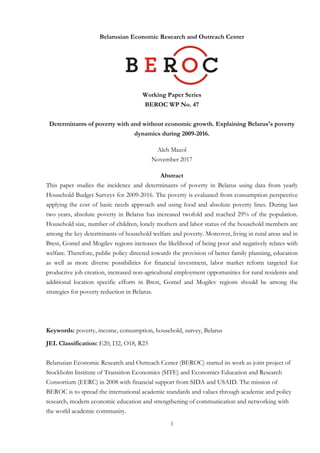
  • 20. 20 current account balance (see Table 4), extensive government ownership of productive enterprises (generate approximately 70% of GDP)18 and direct inference of the state in the economic process. Moreover, the period from 2000 to 2014 also observed a significant increase in real wages in Belarus. As the Table 4 indicates, the real average monthly wages rose from 58900 Belarusian rubles (in constant 2000 prices) in 2000 to 285000 Belarusian rubles in 2014 or by 384% (12% per year on average). This increase in wages reflects growth in social spending that helped to reduce poverty and inequality (see Mazol, 2016). However, it also build a significant ground for macroeconomic imbalances19 that coupled with expansionary monetary policy promoting fixed investment (see Table 4), an appreciation in the real exchange rate, subsidized prices for key inputs (including energy and utilities) and favored treatment for state-owned enterprises in access to "cheap" finance targeted at their production growth led to financial crisis in 2011, subsequent recession in 2012-2014 and economic crisis in 2015-2016 (Dobrinsky et al., 2016). Turning to poverty, trends in its incidence (headcount index) based on absolute poverty line are illustrated in Figure 1. Subsequently, as can be seen from the graph, the timeline of poverty analysis for Belarus can be subdivided into three periods: 2009-2011, 2012-2014, and 2015-2016. Figure 1: Incidence of absolute poverty and GDP per capita growth in Belarus Source: authors estimates based on BHBS-2009, BHBS-2010, BHBS-2011, BHBS-2012, BHBS-2013, BHBS-2014, BHBS-2015, BHBS-2016. Note: Estimates reflect weighted household data. 18 The state sector in Belarus dominates especially in the manufacturing sector, whereas the private sector concentrate mostly in retail trade and business services. 19 Forced growth of wages resulted in significant increase of unit labor costs (real wage growth outperformed productivity growth), competitiveness losses and was one of the main sources of inflationary pressure in the economy of Belarus (Dobrinsky et al., 2016). -10% 0% 10% 20% 30% 40% 50% 2009 2010 2011 2012 2013 2014 2015 2016 0.4 7.9 5.7 1.8 1.0 1.6 -4.0 -2.8 National headcount index, % Rural headcount index, % Urban headcount index, % GDP per capita growth, %
  • 21. 21 During the first period (from 2009 to 2011), absolute poverty at the national level increased from 30.9% to 32.6%. Incidence of absolute poverty for rural and urban areas in 2011 reached 45% and 28% of the population, correspondingly. In the spatial dimension, the highest level in the incidence of absolute poverty in 2011 was in Brest, Gomel and Mogilev regions – 38.9%, 39.4% and 40.9%, correspondingly (see Table A6). From 2009 to 2011, the depth and strength of absolute poverty stayed almost unchanged, as it is apparent from the dynamics of poverty gap index and poverty severity index (see Table 5). The poverty gap index decreased from 13.2% to 13% for rural areas, while it increased for urban areas – from 6.2% to 6.4%. The dynamics of poverty severity index followed the same pattern – slightly decreasing for rural areas and increasing for urban areas. However, overly the above figures indicate the seriousness of absolute poverty in Belarus during the first studied period especially for rural areas. Table 5. Poverty measures based on absolute poverty line by area and year in Belarus Year Poverty measure 2009 2010 2011 2012 2013 2014 2015 2016 Headcount index (P0), % National 30.917 27.387 32.581 23.431 15.272 14.874 22.483 29.297 Rural 42.524 40.277 44.505 31.768 23.974 22.398 34.058 40.547 Urban 26.861 22.645 28.324 20.405 12.225 12.114 18.450 25.271 Poverty gap (P1), % National 8.027 6.850 8.160 5.586 3.374 3.272 5.240 7.078 Rural 13.185 11.551 12.988 8.406 6.056 5.583 8.878 11.233 Urban 6.225 5.121 6.436 4.563 2.435 2.425 3.973 5.591 Poverty severity (P2), % National 3.170 2.555 3.090 2.003 1.167 1.082 1.853 2.529 Rural 5.914 4.756 5.334 3.252 2.261 2.068 3.324 4.387 Urban 2.211 1.746 2.289 1.550 0.784 0.720 1.340 1.865 Source: authors estimates based on BHBS-2009, BHBS-2010, BHBS-2011, BHBS-2012, BHBS-2013, BHBS-2014, BHBS-2015, BHBS-2016. Note: Estimates reflect weighted household data. The dynamics of food poverty based on corresponding food poverty line during 2009-2011 is illustrated in Figure 2. Determining food poverty as the consumption expenditure necessary to cover the cost of the minimum nutritional requirement (basic need food items), food poverty at the national level decreased from 3.1% in 2009 to 2.9% in 2011. However, this drop corresponds only to rural area, while urban area showed increase in incidence of food poverty. Nonetheless, food poverty disproportionally affected rural households. The ratio of food poverty headcount indices for the rural and urban areas ( 0 0 rural urban P P ) was 4.8 in 2009, 4.0 in 2010, and 3.3 in 2011. The highest regional levels in the incidence of food poverty in 2011 were in Gomel and Mogilev regions – 4.9% for both regions (see Table A3).
  • 22. 22 Figure 2: Incidence of food poverty in Belarus Source: authors estimates based on BHBS-2009, BHBS-2010, BHBS-2011, BHBS-2012, BHBS-2013, BHBS-2014, BHBS-2015, BHBS-2016. Note: Estimates reflect weighted household data. The dynamics of corresponding poverty gap and poverty severity indices of food poverty share the same pattern of headcount index (see Table 6) – decreasing at the national and rural levels, and slightly increasing at the urban level. Table 6. Poverty measures based on food poverty line by area and year in Belarus Year Poverty measure 2009 2010 2011 2012 2013 2014 2015 2016 Headcount index (P0), % National 3.147 2.329 2.890 1.320 0.541 0.411 0.656 1.116 Rural 7.718 5.236 5.901 2.729 1.225 1.239 1.472 2.473 Urban 1.549 1.259 1.815 0.809 0.301 0.108 0.372 0.631 Poverty gap (P1), % National 0.683 0.371 0.540 0.223 0.078 0.041 0.114 0.144 Rural 1.833 0.996 1.093 0.501 0.161 0.120 0.274 0.322 Urban 0.280 0.141 0.343 0.122 0.049 0.011 0.058 0.081 Poverty severity (P2), % National 0.216 0.095 0.168 0.059 0.017 0.006 0.034 0.030 Rural 0.626 0.282 0.344 0.124 0.028 0.020 0.087 0.066 Urban 0.072 0.026 0.105 0.036 0.014 0.001 0.015 0.017 Source: Authors estimates based on BHBS-2009, BHBS-2010, BHBS-2011, BHBS-2012, BHBS-2013, BHBS-2014, BHBS-2015, BHBS-2016. Note: Estimates reflect weighted household data. 0% 1% 2% 3% 4% 5% 6% 7% 8% 2009 2010 2011 2012 2013 2014 2015 2016 National headcount index, % Rural headcount index, % Urban headcount index, %
  • 23. 23 The second period (from 2012 to 2014) was characterized by a sharp poverty reduction (see Figure 1). For example, the absolute national poverty headcount ratio has plummeted from 32.6% in 2011 to 14.9% in 2014, rural poverty dropped by 22.1 percentage points or almost by half and urban poverty decreased by 16.2 percentage points. Correspondingly, the depth and strength of absolute poverty decreased as well: the poverty gap index by 4.9 percentage points and the poverty severity index by 2 percentage points. Within each year of the second period, absolute poverty rates lowered as the measure of household income becomes more significant (see Figure 3). As graph shows, the real per capita household income increased by 39% from 2011 to 2014. However, the headcount ratio remains higher in the rural than in the urban area, the two ratios were not converging – the ratio ( 0 0 rural urban P P ) increased from 1.6 in 2011 to 1.9 in 2014 (see Table 6). All these suggest the existence of the disintegrated labor market in Belarus during second period, and indicates that non-agricultural sources of income are not the same in the two areas. Figure 3: Household income and expenditure share on food in Belarus Source: authors estimates based on BHBS-2009, BHBS-2010, BHBS-2011, BHBS-2012, BHBS-2013, BHBS-2014, BHBS-2015, BHBS-2016. Note: Real total household income is the household average real monthly per capita income received by all household members and comprises monetary income as well as the monetary value of income received in the form of goods and services (the monetary assessment of in-kind payments obtained by the respondents)20. Estimates reflect weighted household data. In the spatial dimension, the highest levels in the incidence of absolute poverty in 2014 were in Brest, Gomel and Mogilev regions – 18.3%, 18.4% and 25.0%, correspondingly (see Table A6). 20 Household income is the sum of labor earnings [a. any payments after taxes from main and additional jobs of all household members in the form of money, goods or services + b. income from sale of own produced products, including food and animals not included in a.], capital earnings [income from capital investment + income from sale of personal property (assets) + income from renting apartment(s)/house(s) or other personal property], government transfers [any type of pension (retirement pension, pension for years of service, disability pension, loss of provider pension) + unemployment benefits + child benefits + other forms of social support (maternity benefits, low-income family benefits, etc.) + stipends], private transfers [help and gifts from relatives and friends in the form of money, goods or services + alimony] + other income. 500000 600000 700000 800000 900000 1000000 20% 24% 28% 32% 36% 40% 2009 2010 2011 2012 2013 2014 2015 2016 Real total household income, in BYN 2009 (left axis) Average household expenditure share on food (right axis) 28.6 26.9 27.7 26.2 23.1 23.9 24.6 25.3
  • 24. 24 The estimates of food poverty also showed substantial improvement: its incidence dropped from 2.9% in 2011 to 0.4% in 2014 (see Table 6). The same happened for rural and urban areas: the headcount ratio declined and equaled 1.2% for rural areas and 0.1% for urban areas in 2014. The progress in food poverty showed all regions of Belarus. Finally, during the second period, the depth and strength of absolute and food poverty also decreased substantially at national level, both for urban and rural areas and for all Belarusian regions (see Table A2 and A3). This is not surprising, since rapid increase in real per capita household income in Belarus led to rise in calorie intake and, thus, real per capita household expenditure. In turn, the third period saw a sharp rise in the incidence of poverty. From 2015 to 2016, the headcount ratio for absolute poverty increased by 14.4 percentage points (see Table 5). As a result, in 2016 the share of expenditure-poor households in Belarus reached 29.3% or almost the same as in 2009 and 2011. The incidence of food poverty was growing moderately – from 0.4% in 2014 to 1.1% in 2016 (see Table 6). Moreover, during the third period not only urban and rural disparity for poverty widened – 25.3% in urban vs 40.6% in rural areas in 2016 and for extreme poverty – 0.6% vs. 2.5%, but also regional variations in both absolute and extreme poverty were also large (see Table A6 and A7). Brest and Mogilev regions showed 38.3% and 35.6% of incidence of absolute poverty, respectively, while only 12.3% of households in Minsk city were observed to be overly poor. The same holds for depth and strength of absolute poverty. The significant increase in poverty in 2015-2016 was due to a combination of several factors, including the household income decline in comparison with its growth in previous years, the increasing need to spend more on food necessities (see Figure 3) and the growth in food and especially non-food price levels (see Figure 4). Figure 4: Real monthly average per capita household expenditure on food and non-food items and real monthly standardized food and non-food poverty lines, 2009-2016 180000 200000 220000 240000 260000 280000 300000 320000 100000 200000 300000 400000 500000 600000 700000 800000 2009 2010 2011 2012 2013 2014 2015 2016 Food poverty line (left axis) Non-food poverty line (left axis) Real expenditure on food (right axis) Realexpenditure on non-food items (right axis)
  • 25. 25 Source: Authors estimates based on BHBS-2009, BHBS-2010, BHBS-2011, BHBS-2012, BHBS-2013, BHBS-2014, BHBS-2015, BHBS-2016. Note: In constant prices (2009=100). Poverty lines presented on the graph were defined for the comparison purposes and calculated per standardized person (assuming 2100 kcal/day). Estimates reflect weighted household data. As the Figure 4 shows, starting from 2015 there has been a rapid increase in the real cost of non- food budget for Belarusian households, while cost of food budget have remained almost the same in real terms. Correspondingly, the non-food poverty line increased from 267074 Belarusian rubles in 2014 to 306156 Belarusian rubles in 2016 or by 14.6%, while the food poverty line increased only by 2.9%. Furthermore, as income fell (by 7.2% over the 2015-2016), the share of food items in total expenditure increased (see Figure 3) and real non-food expenditure decreased. This is because household income was not enough to cover both expenditures on food and non-food items. As a result, due to 2015-2016 economic crisis the cost of meeting the non-food essentials has increased so fast (see Figure 4) that it has squeezed the non-food budget, leaving insufficient purchasing power for non-food items. Finally, in order to be consistent with the results above Figure 5 displays the cumulative distribution functions of real monthly per capita household expenditure for five surveys with the 2009 as the base year. The figure shows a shift in the whole distribution of household expenditure in Belarus from one year to the next, except for that of 2016, which demonstrates the downward dynamics and tends to that of 2012. Figure 5: Cumulative distribution functions of real monthly per capita household expenditure for 2009, 2011, 2012, 2014 and 2016 Source: Authors estimates based on BHBS-2009, BHBS-2010, BHBS-2011, BHBS-2012, BHBS-2013, BHBS-2014, BHBS-2015, BHBS-2016. 5.2. OLS regression results: determinants of welfare Table 7 presents the regression results for the correlates of household welfare in 2009 -2016 measured by the log of real household per capita consumption in terms of 2009 Belarusian rubles. Because the dependent variable is in the log form, the calculated regression coefficients for 0.0 0.2 0.4 0.6 0.8 1.0 11.50 12.00 12.50 13.00 13.50 14.00 14.50 15.00 15.50 2009 2011 2012 2014 2016 Probability 2009 2016
  • 26. 26 continuous variables measure the percentage change in household per capita consumption due to a unit increase in the independent variable. For categorical (dummy) variables, the percentage change in per capita consumption due to the change in the considered binary variable from a value of 0 to 1 was estimated as follows: 100·(ea -1), where a denotes the calculated coefficient for the considered independent variable (Giles, 2011).
  • 27. 27 Table 7. OLS estimates of log of household per capita consumption (welfare) Variable 2009 2010 2011 2012 2013 2014 2015 2016 Household size -0.098*** [0.024] -0.110*** [0.023] -0.139*** [0.022] -0.185*** [0.021] -0.179*** [0.025] -0.133*** [0.022] -0.195*** [0.027] -0.215*** [0.023] Household size squared 0.007* [0.004] 0.011*** [0.003] 0.015*** [0.003] 0.020*** [0.003] 0.021*** [0.004] 0.008** [0.004] 0.018*** [0.004] 0.025*** [0.004] Age of head 0.011*** [0.004] 0.003 [0.003] 0.006* [0.003] 0.006* [0.003] 0.007** [0.003] 0.015*** [0.003] 0.009 [0.006] 0.014*** [0.004] Age of head squared * 103 -0.141*** [0.038] -0.074*** [0.028] -0.107*** [0.032] -0.094*** [0.029] -0.117*** [0.030] -0.188*** [0.029] -0.130*** [0.050] -0.180*** [0.032] Number of children of age 0-5 -0.217*** [0.021] -0.197*** [0.021] -0.240*** [0.022] -0.181*** [0.020] -0.169*** [0.020] -0.120*** [0.024] -0.119*** [0.029] -0.161*** [0.025] Number of children of age 6-12 -0.205*** [0.019] -0.206*** [0.017] -0.195*** [0.017] -0.212*** [0.018] -0.198*** [0.019] -0.163*** [0.022] -0.189*** [0.026] -0.210*** [0.021] Number of children of age 13-17 -0.067*** [0.018] -0.079*** [0.020] -0.080*** [0.020] -0.040* [0.021] -0.069*** [0.022] -0.041* [0.024] -0.096*** [0.030] -0.100*** [0.025] Number of pensioners -0.079*** [0.014] -0.043*** [0.013] -0.023* [0.013] -0.065*** [0.014] -0.047*** [0.014] -0.010 [0.014] -0.012 [0.013] -0.005 [0.017] Average years of schooling (15-72) 0.041*** [0.002] 0.039*** [0.002] 0.033*** [0.002] 0.039*** [0.002] 0.036*** [0.002] 0.038*** [0.002] 0.024*** [0.002] 0.047*** [0.002] HH with only woman and children -0.196*** [0.038] -0.194*** [0.035] -0.158*** [0.038] -0.104*** [0.034] -0.199*** [0.033] -0.215*** [0.032] -0.204*** [0.032] -0.154*** [0.029] Inactive -0.070*** [0.019] -0.093*** [0.019] -0.102*** [0.023] -0.144*** [0.021] -0.131*** [0.020] -0.108*** [0.021] -0.106*** [0.024] -0.096*** [0.022] Access to landplot 0.089*** [0.018] 0.103*** [0.017] 0.087*** [0.018] 0.107*** [0.017] 0.059*** [0.017] 0.065*** [0.017] 0.087*** [0.019] 0.072*** [0.019] Savings 0.124*** [0.016] 0.130*** [0.016] 0.152*** [0.014] 0.181*** [0.015] 0.183*** [0.016] 0.160*** [0.015] 0.155*** [0.014] 0.138*** [0.015] Brest region (OV: Minsk region) -0.122*** [0.025] -0.057** [0.024] -0.095*** [0.025] -0.173*** [0.022] -0.133*** [0.023] -0.148*** [0.026] -0.126*** [0.024] -0.089*** [0.024] Vitebsk region -0.072*** [0.027] -0.048* [0.025] -0.074*** [0.026] -0.152*** [0.024] -0.126*** [0.024] -0.137*** [0.025] -0.071*** [0.023] -0.079*** [0.022] Grodno region -0.049* [0.026] -0.024 [0.025] -0.086*** [0.023] -0.091*** [0.026] -0.091*** [0.025] -0.121*** [0.026] -0.043* [0.023] -0.040* [0.023] Gomel region -0.114*** [0.026] -0.142*** [0.024] -0.079*** [0.025] -0.168*** [0.023] -0.176*** [0.025] -0.152*** [0.024] -0.102*** [0.023] -0.074*** [0.023] Mogilev region -0.169*** [0.027] -0.159*** [0.026] -0.169*** [0.028] -0.158*** [0.024] -0.193*** [0.026] -0.188*** [0.026] -0.121*** [0.024] -0.096*** [0.022] Town (OV: village) 0.082*** [0.019] 0.127*** [0.017] 0.091*** [0.017] 0.079*** [0.018] 0.090*** [0.018] 0.062*** [0.018] 0.072*** [0.018] 0.068*** [0.017] City 0.200*** [0.019] 0.199*** [0.018] 0.167*** [0.018] 0.123*** [0.017] 0.136*** [0.018] 0.134*** [0.019] 0.175*** [0.017] 0.148*** [0.016] Minsk 0.304*** [0.028] 0.331*** [0.026] 0.271*** [0.026] 0.179*** [0.025] 0.199*** [0.026] 0.215*** [0.029] 0.396*** [0.028] 0.321*** [0.025] Constant 12.681*** [0.097] 12.976*** [0.089] 13.097*** [0.088] 13.248*** [0.089] 13.409*** [0.093] 13.190*** [0.095] 13.477*** [0.157] 12.988*** [0.116] Observations 4535 5006 4949 4803 4971 5123 5350 5367 R2 0.414 0.390 0.385 0.401 0.368 0.398 0.369 0.406 Note: Results reflect weighted household data. Robust standard errors in square brackets. *** significant at 1%, ** significant at 5%, * significant at 10%.
  • 28. 28 The goodness-of-fit statistics R2 indicate a reasonably good fit for all model specifications. The F- statistics are highly significant (p < 0.001), indicating that the explanatory variables jointly exert significant influence on household welfare. Furthermore, most of the estimated coefficients are strongly significant during all studied years. As shown in Table 7, household size has a statistically significant and relatively large negative impact on welfare of household in Belarus during all years, meanwhile substantially increasing in 2012 – the year after the 2011 domestic financial crisis and in 2015-2016 – period of economic crisis. The coefficients of the households size are -0.185 in 2012, -0.195 in 2015 and -0.215 in 2016. This means that the increase in the size of the household decreases its real per capita expenditure (consumption) by 18.5% in 2012, by 19.5% in 2015 and by 21.5% in 2016. Moreover, the Belarusian households' size profile is concave (the coefficients for household size squared are positive). The coefficients of the age of the household head are positive and significant for all studied years except 2010 and 2015. In turn, squared of household head is negative and significant. These mean that the older heads increase household welfare in Belarus, but as age of household's head increases the welfare of the household increases at a decreasing rate, reaches a maximum, and decreases at old age. These results confirm findings of the previous studies for other countries, in particular are consistent with life-cycle hypothesis of higher earning capacity with greater experience and smoothing of consumption over the life cycle. However, the magnitude of the age of the household head coefficients is relatively low (see Table 7), indicating that that Belarusian households headed by older individuals, holding other variables constant, will not tend to have substantially higher welfare than those headed by younger individuals. The increase in the number of children in the Belarusian households has significant and relatively large negative effect on household per capita expenditure during all studied years. However, the impact is noticeably higher for children in the age of 0-5 and 6-12, than in the age of 13-17. Moreover, starting from 2012 the influence of number of children in the age of 6-12 on welfare of household is the highest one (see Table 7). These results may indicate, first, that the presence of more children in a Belarusian household implies a lower share of adult members in employment, which constraints the earning potential of that household. Second, Belarusian families with more children in the age of 6-12 bear larger cost burden (especially starting from 2012), such as the cost of education, health care or other costs concerning children than families with more children in the age of 0-5 (to a lesser extent) and in the age of 13-17 (to a greater extent). As Table 7 displays, the increase in the number of household's members in the pension age in Belarus has significant negative effect on real household per capita consumption, but only in 2009- 2013. Staring from 2014 the influence is insignificant. Such factor as average years of schooling of the household is positively correlated with household per capita consumption. For example, a one-year increase in schooling resulted in 4.1% increase in per capita consumption in 2009, 3.9% in 2012 and 4.7% in 2016, suggesting that attainment of higher levels of education provides higher levels of household welfare. This is expected as an
  • 29. 29 increase in educational attainments increases the chances of one's absorption in the labor market and increased earnings. However, overly, the influence of level of education on household's welfare does not exceed 5% for all studied years, which is low in comparison with other correlates (and other countries, especially developed) suggesting the presence of educational inefficiency in the labor market of Belarus.21 The results also indicate that households with children, whose heads are lonely mothers gained substantially lower per capita consumption, for example, by 21.7% in 2009, by 11.0% in 2012 and by 16.8% in 2016. Therefore, in general, these findings suggest, first, that marriage is associated with significantly better economic welfare of members of the households including children (Waite, 1995), and, second, incomplete families should be treated as one of the primary goals for poverty alleviation policy in Belarus. Households having economically inactive members were significantly worse off over the whole studied period and especially in 2012 and 2013 (after the 2011 financial crisis), when its magnitude reached -0.144 and -0.131, correspondingly; meaning 15.5% decrease in household per capita expenditure in 2012 and 14.0% – in 2013. Overly, the presence in the Belarusian family of at least one economically inactive member leads to a large decrease in welfare during all studied years. Access to landplot and savings have a positive impact on real per capita household expenditure meaning that possession of additional physical capital (agricultural assets) and financial capital (bank deposits) help to increase welfare for Belarusian households. However, the effect of financial assets is diminishing in the last three years (2014-2016), while in the period of 2009-2013 it was increasing. These results may be explained due to influence of economic crisis in 2015-2016 preceded by recession, that, first, slowed down the growth of households' incomes in 2014 and, second, led to their decrease in 2015-2016. Additionally, the decrease in the positive influence of savings on welfare of households in Belarus possibly indicates the growing tendency to smooth consumption by Belarusian households through using their savings. However, the longer the crisis or subsequent economic stagnation, the lower the possibilities to smooth consumption – lower savings. In the spatial dimension, the largest negative influence on welfare of household in Belarus showed residence in Brest, Gomel and Mogilev regions especially during 2012-2014. However, starting from 2015 the gap between six regions started to diminish resulted from economic crisis of last two years. Finally, urban residence have a positive impact on real per capita expenditures (see Table 7). For example, households living in cities achieved 22.1%, 13.0% and 16.1% higher per capita consumption in 2009, 2012 and 2016 than rural households. This indicates insufficient employment opportunities, infrastructure, and quality of services in rural areas. Furthermore, it also implies that agriculture, though playing a crucial role as a source of rural livelihood in Belarus, has performed poorly during 2009-2016. 21 The availability of employment opportunities is an important part of the social contract in Belarus. The first objective of public policies in the labor market is the access to jobs for everyone as well as rising personal income through wage growth. The second one is the absence of significant wage differentials achieved using wage scale that regulates the salaries for every profession (Dobrinsky et al., 2016).
  • 30. 30 5.3. Probit regression results: determinants of poverty As a final step, I estimated the determinants of the probability of the Belarusian households to be below the absolute poverty line using probit regression. Table 8 reports the marginal effects for all households and for all studied years. The marginal effect represents the change in the probability of being poor, when a dummy variable changes value from 0 to 1 or a continuous variable changes by one unit. The log-likelihood ratio (LR) tests show that there are significant relationship between the probabilities of being poor and the explanatory variables included in all eight models (p < 0.001). The results in Table 8 highlight that household size and household size squared have coefficients with opposite signs and both are statistically significant. The coefficients for household size are positive suggesting that the probability of households in Belarus being poor increases with the size of the household. The squared term is negative and significant, indicating that the negative effect of household size decreases for bigger households. These relationships hold for all estimated models. Moreover, the effects are much larger in 2012, 2015-2016 than in the rest of the studied years. In the first case, this is a year after the financial crisis in Belarus. In the second case, these are the years of economic crisis. Age of the household head and age squared show insignificant coefficients for all studied years, indicating that the level of household poverty in Belarus does not seem to be determined by the age of the head. Households with more children of age 6-12 are more likely to fall into poverty in Belarus. These results hold over all studied years and possibly indicate that such families bear significant burden, such as the cost of education, health care or other costs concerning children of age 6-12. Moreover, these may also mean that the higher the number of younger (school age) siblings, the greater will be the workload for the adult (working age) members of the households in Belarus, thus higher poverty. On the other hand, there is almost no significant effect on probability of being poor for households with more children over the age of 12 for all studied years except 2009. This may be due to the effect of household help, which means that older children also help in caring for younger siblings in the households. After all, older women are less likely to have younger kids in need of direct care. The marginal effects from Table 8 show that the presence of household members in the pension age decreases the risk of poverty for the Belarusian households with statistically significant effects in 2010-2011 and in 2015-2016. Therefore, presence of more elders in the Belarusian family plays an important role for poverty insurance and especially in periods of financial and economic instability. Next, the higher level of education have a negative, but small impact on the probability of being poor. A one-year increase in schooling resulted in 2.8 percentage points decrease in the probability of being poor in 2009, in 2.4 percentage points in 2012 and 3 percentage points in 2016. Hence, it seems that education in Belarus only slightly improves the skills of individuals leading to small growth of their possibility of obtaining a job and earnings capacity.
  • 31. 31 Table 8. Probit estimates of the determinants of poverty Variable 2009 2010 2011 2012 2013 2014 2015 2016 Household size 0.116*** [0.030] 0.094*** [0.022] 0.102*** [0.032] 0.162*** [0.024] 0.107*** [0.022] 0.070*** [0.023] 0.171*** [0.026] 0.222*** [0.024] Household size squared -0.009* [0.005] -0.006* [0.003] -0.006 [0.005] -0.015*** [0.004] -0.011*** [0.003] -0.002 [0.003] -0.014*** [0.003] -0.021*** [0.004] Age of head 0.0001 [0.004] -0.002 [0.003] 0.005 [0.004] -0.001 [0.003] 0.004 [0.003] 0.002 [0.003] -0.001 [0.003] -0.005 [0.004] Age of head squared * 103 -0.001 [0.038] 0.016 [0.030] -0.052 [0.035] 0.004 [0.031] -0.039 [0.030] -0.021 [0.031] 0.005 [0.031] 0.055 [0.037] Number of children of age 0-5 0.057** [0.023] 0.019 [0.018] 0.077*** [0.025] 0.001 [0.020] -0.007 [0.019] -0.036* [0.018] -0.039* [0.021] -0.023 [0.025] Number of children of age 6-12 0.099*** [0.019] 0.086*** [0.015] 0.107*** [0.020] 0.083*** [0.018] 0.066*** [0.014] 0.048*** [0.014] 0.081*** [0.017] 0.076*** [0.022] Number of children of age 13-17 0.062*** [0.019] 0.018 [0.017] 0.003 [0.022] 0.002 [0.019] 0.017 [0.017] 0.010 [0.017] 0.031 [0.021] 0.039 [0.024] Number of pensioners -0.015 [0.018] -0.032** [0.015] -0.040** [0.016] -0.012 [0.015] -0.010 [0.013] -0.010 [0.013] -0.027* [0.015] -0.057*** [0.018] Average years of schooling (15-72) -0.028*** [0.002] -0.027*** [0.002] -0.028*** [0.002] -0.024*** [0.002] -0.018*** [0.002] -0.014*** [0.002] -0.013*** [0.002] -0.030*** [0.003] HH with only woman and children 0.087** [0.035] 0.118*** [0.031] 0.114*** [0.031] 0.036 [0.030] 0.083*** [0.025] 0.085*** [0.023] 0.089*** [0.027] 0.074** [0.030] Inactive 0.049** [0.019] 0.061*** [0.017] 0.092*** [0.023] 0.099*** [0.018] 0.080*** [0.016] 0.070*** [0.015] 0.063*** [0.019] 0.080*** [0.022] Access to landplot -0.060*** [0.019] -0.069*** [0.017] -0.066*** [0.019] -0.049*** [0.017] -0.034** [0.016] -0.045*** [0.015] -0.060*** [0.017] -0.088*** [0.019] Savings -0.092*** [0.015] -0.096*** [0.014] -0.118*** [0.015] -0.128*** [0.013] -0.101*** [0.012] -0.100*** [0.013] -0.095*** [0.014] -0.105*** [0.015] Brest region (OV: Minsk region) 0.102*** [0.027] -0.011 [0.023] 0.101*** [0.025] 0.119*** [0.023] 0.064*** [0.021] 0.057*** [0.021] 0.064*** [0.025] 0.066** [0.027] Vitebsk region 0.058** [0.029] 0.008 [0.024] 0.058*** [0.027] 0.118*** [0.024] 0.048** [0.023] 0.059*** [0.022] 0.055** [0.024] 0.046 [0.029] Grodno region 0.011 [0.029] -0.013 [0.024] 0.040 [0.028] 0.019 [0.031] -0.004 [0.023] 0.024 [0.025] -0.023 [0.027] 0.008 [0.028] Gomel region 0.081*** [0.027] 0.062*** [0.022] 0.082*** [0.026] 0.126*** [0.023] 0.090*** [0.022] 0.070*** [0.021] 0.058** [0.025] 0.045* [0.026] Mogilev region 0.154*** [0.029] 0.115*** [0.024] 0.142*** [0.028] 0.104*** [0.025] 0.085*** [0.023] 0.111*** [0.022] 0.052* [0.027] 0.085*** [0.028] Town (OV: village) -0.055*** [0.018] -0.076*** [0.016] -0.066*** [0.019] -0.029 [0.017] -0.060*** [0.015] -0.039** [0.015] -0.076*** [0.020] -0.066*** [0.020] City -0.138*** [0.019] -0.125*** [0.017] -0.117*** [0.019] -0.085*** [0.017] -0.090*** [0.015] -0.074*** [0.015] -0.141*** [0.016] -0.125*** [0.018] Minsk -0.121*** [0.033] -0.230*** [0.029] -0.117*** [0.030] -0.103*** [0.030] -0.074*** [0.026] -0.080*** [0.027] -0.220*** [0.031] -0.204*** [0.031] Observations 4535 5006 4949 4803 4971 5123 5350 5367 Pseudo R2 0.213 0.239 0.220 0.235 0.214 0.263 0.238 0.256 Note: Results reflect weighted household data. Robust z statistics in square brackets. *** significant at 1%, ** significant at 5%, * significant at 10%.
  • 32. 32 In contrast, the results of this study show that incomplete family is very important and significant determinant of poverty in Belarus. During 2009-2016, being a lonely mother with children increases the probability of being poor, for example, by 8.7 percentage points in 2009, by 11.4 percentage points in 2011 and by 7.4 percentage points in 2016. As Table 8 shows, both access to landplot and savings reduce the probability of being poor for Belarusian families. Besides that, all coefficients for variable indicating presence of the inactive member in the household are positive and statistically significant indicating increase in the likelihood of being poor for such households in Belarus. Furthermore, the probit results also indicate that, relative to rural areas, families in urban areas and especially in Minsk are less vulnerable to poverty. Moreover, in 2015-2016 the last link increased substantially, indicating more job and higher earnings opportunities in Belarusian capital in period of economic crisis. In turn, households living in rural areas mostly dependent on agriculture that do not have many employment opportunities. Therefore, the poverty alleviation strategies are more urgent in rural areas and in small cities of Belarus especially in years of economic turbulence. Finally, poverty in Belarus has also a spatial dimension. Families living in Mogilev, Gomel and Brest regions have substantially higher probabilities of being poor than in the rest of Belarusian regions. 7. Conclusion Poverty alleviation and development reflect economic and social progress in the country. Therefore, understanding the pattern of poverty and its driving mechanism through which poverty arises and expands can provide valuable insights into the design of pro-poor policies. Consequently, this paper provides an assessment of poverty in Belarus based on household consumption expenditure and using eight waves of surveys to track the dynamics of poverty change across three development periods: 2009-2011, 2012-2014, and 2015-2016. It was assumed that different macroeconomic conditions followed each of these episodes have differential effects on poverty during the respective periods. The study used the cost of basic needs approach to calculate food and absolute poverty lines for each sampled household over eight years and across all regions of Belarus. An analysis of poverty was performed at the level of entire Belarus and its constituent parts based on Foster-Greer-Thorbecke's poverty indices and using OLS and probit regressions. Several sets of conclusions can be drawn. First, during 2009-2011, poverty at the national level stayed almost unchanged. The 2011 financial crisis was associated with a slight increase in the incidence of poverty, but not the depth and severity of poverty. During 2012-2014 there was a substantial decrease in incidence of poverty (by 18 percentage points) caused mostly by the strong growth of household incomes (by 39%). In contrast, economic crisis in 2015-2016 was associated with a twofold increase in incidence, depth and severity of poverty in Belarus.
  • 33. 33 Second, the other outcome of the poverty measures undoubtedly points out that considerably more poverty exists in the nation's rural areas than in urban areas. For instance, the poverty incidence for the nation's rural areas over 2009-2016 is approximately 10.5 percentage points (or 44%) higher than the national average, while that of the urban areas is nearly 4 percentage points (or 16%) below national average. These suggest the presence of significant inequality, with poorer rural households falling to benefit from the more remunerative productive activities. The higher income households tend to be very concentrated in the urban centers of Belarus, where many of these productive activities are based. Moreover, high levels of poverty in rural areas possibly reflect the limited employment opportunities available to households in these areas. Therefore, more immediately, attention needs to be paid to the reduction in urban-rural inequalities, given that poverty in Belarus is disproportionately a rural phenomenon and given that such inequalities are likely to be an important contributory factor to urban poverty as well (through the migration induced as a result). This raises the issue of whether government policy is sufficiently focused on the needs of rural households to overcome the already very strong tendencies toward urban concentration (78% of population). Third, comparing to such urban-rural differences, however, some regional differences are also large. In particular, a poverty incidence for Grodno region in 2016 is roughly 3% below the national average, that for the Brest and Mogilev regions are 31% and 21% higher than this average, correspondingly. Finally, besides describing the pattern of poverty, the second main objective of this paper was to identify some of the most important determinants of welfare and key contributory causes of poverty in Belarus at the household level. Such an analysis provides important general information, which is of value in working out at least some of the key priorities of a poverty alleviation strategy. Among factors that decrease household welfare and increase poverty are household size, the number of children in a household, presence in the household of economically inactive members. The next result is that lonely mothers appear to be substantially more vulnerable to macroeconomic shocks than full families both from welfare and poverty perspectives. By far one of the most important determinants of welfare and poverty in all samples is spatial location of household. Poverty highly discriminates against living in rural areas, Brest, Gomel and Mogilev regions. In turn, on average, positive influence on consumption expenditure and negative on the chance of getting poor have savings and access to landplot. It is supposed that landplot experience increases household welfare, that is reduces the chance of not having adequate food and thereby falling below the minimum calorie intake. Therefore, polices directed towards the provision of better family planning, education as well as more diverse possibilities for financial investment, increased non-agricultural employment opportunities for rural residents and additional location specific efforts in Brest, Gomel and Mogilev regions are important for reducing poverty in Belarus.
  • 34. 34 The further directions of poverty studies in Belarus should include several questions: How much of the differences have been and might be brought down by rapid economic growth? What has been the effectiveness of regional policies and efforts to increase the efficiency of use of regional resources? To what extent can policies to improve the mobility of resources reduce disparities? References Adam, J. (1982). Employment Policies in the Soviet Union and Eastern Europe. London, Macmillan. Aguiar, M. and E. Hurst. (2005). Consumption Versus Expenditure. Journal of Political Economy, 113(5): 919-948. Ando, A. and F. Modigliani. (1963). The Life Cycle Hypothesis of Saving: Aggregate Implications and Tests. American Economic Review, 53(1): 55-84. Angelsen, A., Jagger, P., Babigumira, R., Belcher, B., Hogarth, N.J., Bauch, S., Börner, J., Smith-Hall, C., and S. Wunder. (2014). Environmental Income and Rural Livelihoods: A Global Comparative Analysis. World Development, 64: S12-S28. Aron, J., J. Duca, J. Muellbauer, K. Murata, and A. Murphy. (2010). Credit, Housing Collateral and Consumption: Evidence from the UK, Japan and the US. CEPR Discussion Paper No. 7876. Asselin, L.-M., and A. Dauphin. (2001). Mesure de la Pauvreté: un Cadre Conceptuel [Poverty Measurement: A Conceptual Framework], Centre Canadien d’Etude et de Cooperation International [Canadian Centre for International Studies and Cooperation, Quebec] Bane, M., and D. Ellwood. (1986). Slipping into and Out of Poverty: The Dynamics of Spells. Journal of Human Resources, 21: 1-23. Barrett, C., Reardon, T., and P. Webb. (2001). Nonfarm Income Diversification and Household Livelihood Strategies in Rural Africa: Concepts, Dynamics, and Policy Implications. Food Policy, 26: 315-331. Briggs, Xavier de Souza. (1998). Brown Kids in White Suburbs: Housing Mobility and the Many Faces of Social Capital. Housing Policy Debate, 9(1): 177-221. Brainerd, E. (2000). Women in Transition: Changes in Gender Wage Differentials in Eastern Europe and the Former Soviet Union. Industrial & Labor Relations Review, 54(1): 138-162. Bruck, T., Danzer, A., Muravyev, A. and N. Weisshaar (2010). Poverty During Transition: Household Survey Evidence from Ukraine. Journal of Comparative Economics, 38(2): 123-145. Bucks, B., A. Kennickell, and K. Moore. (2006). Recent Changes in U.S. Family Finances: Evidence from the 2001 and 2004 Survey of Consumer Finances. Federal Reserve Bulletin, A1-A38. Campiglio, L. (2017). Absolute-poverty, Food and Housing. VP vita e pensiero, 79: 1-64.
  • 35. 35 Caner, A. and E. Wolff. (2004). Asset Poverty in the United States, 1984-99: Evidence from the Panel Study of Income Dynamics. Review of Income and Wealth, 50(4): 493-518. Carroll, C. (1997). Buffer Stock Saving and the Life Cycle/Permanent Income Hypothesis. Quarterly Journal of Economics, 112(1): 1-56. Carroll, C., M. Otsuka, and J. Slacalek. (2011). How Large Are Housing and Financial Wealth Effects? A New Approach. Journal of Money, Credit and Banking, 43 (1): 55-79. Chen, S., and M. Ravallion. (2004). How Have the World’s Poorest Fared Since the Early 1980s?. World Bank Research Observer, 19: 141-169. Chen, S., and M. Ravallion. (2010). The Developing World is Poorer Than We Thought, But No Less Successful in the Fight Against Poverty. Quarterly Journal of Economics, 125(4): 1577-1625. Cojocaru, A., and M. Matytsin (2017). Poverty and shared prosperity in Belarus over the past decade: Trends, drivers and challenges. Poverty and Equity Global Practice. Washington DC: The World Bank. Conley, D. (1999). Being Black, Living in the Red. Berkeley: University of California Press. Deaton, A. (1992). Understanding Consumption. Oxford: Oxford University Press. Deaton, A. (1997). The Analysis of Household Surveys: A Microeconometric Approach to Development Policy. Johns Hopkins University Press, Baltimore. Deaton, A. (2003). Measuring Poverty. Research Program in Development Studies, Princeton: Princeton University. Deaton, A. (2008). Income, Health, and Well-Being around the World: Evidence from the Gallup World Poll. Journal of Economic Perspectives, 22(2): 53-72. Dercon, S. (1996). Risk, Crop Choice and Savings: Evidence from Tanzania. Economic Development and Cultural Change, 44(3): 385-514. Dercon, S. and K. Pramilla. (1996). Income Portfolios in Rural Ethiopia and Tanzania: Choices and Constraints. Journal of Development Studies, 32(6): 850-875. Dollar D. and A. Kraay. (2002). Growth is Good for the Poor. Journal of Economic Growth, 7(3): 195- 225. Dobrinsky R., Adarov A., Bornukova K., Havlik P., Hunya G., Kruk D., and O. Pindyuk. (2016). The Belarus Economy: The Challenges of Stalled Reforms. wiiw Research Report No. 413. The Vienna Institute for International Economic Studies, Vienna, Austria. Easterly W. and S. Fischer. (2001). Inflation and the Poor. Journal of Money, Credit and Banking, 33(2): 160-178. Ellis, F. (2000). The Determinants of Rural Livelihood Diversification in Developing Countries. Journal of Agricultural Economics, 51: 289-302.