Downloaded 20 times
![Previous work
Topic models: latent Dirichlet allocation (LDA) [Barnard et
al. ’03], Machine Translation [Duygulu et al. ’02]
Mixture models: Continuous Relevance Model (CRM)
[Lavrenko et al. ’03], Multiple Bernoulli Relevance Model
(MBRM) [Feng ’04]
Discriminative models: Support Vector Machine (SVM)
[Verma and Jahawar ’13], Passive Aggressive Classifier
[Grangier ’08]
Local learning models: Joint Equal Contribution (JEC)
[Makadia’08], Tag Propagation (Tagprop) [Guillaumin et al.
’09], Two-pass KNN (2PKNN) [Verma et al. ’12]](https://image.slidesharecdn.com/sklcrmtalk-140403051314-phpapp02/85/Sparse-Kernel-Learning-for-Image-Annotation-5-320.jpg)
![Continuous Relevance Model (CRM)
CRM estimates joint distribution of image features (f) and
words (w)[Lavrenko et al. 2003]:
P(w, f) =
J∈T
P(J)
N
j=1
P(wj |J)
M
i=1
P(fi |J)
P(J): Uniform prior for training image J
P(fi |J): Gaussian non-parametric kernel density estimate
P(wi |J): Multinomial for word smoothing
Estimate marginal probability distribution over individual tags:
P(w|f) =
P(w, f)
w P(w, f)
Top e.g. 5 words with highest P(w|f) used as annotation](https://image.slidesharecdn.com/sklcrmtalk-140403051314-phpapp02/85/Sparse-Kernel-Learning-for-Image-Annotation-10-320.jpg)


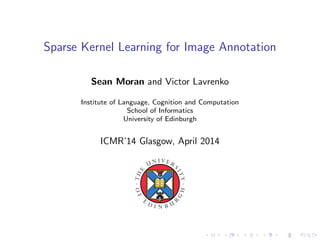
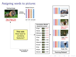
![Datasets/Features
Standard evaluation datasets:
Corel 5K: 5,000 images (landscapes, cities), 260 keywords
IAPR TC12: 19,627 images (tourism, sports), 291 keywords
ESP Game: 20,768 images (drawings, graphs), 268 keywords
Standard “Tagprop” feature set [Guillaumin et al. ’09]:
Bag-of-words histograms: SIFT [Lowe ’04] and Hue [van de
Weijer & Schmid ’06]
Global colour histograms: RGB, HSV, LAB
Global GIST descriptor [Oliva & Torralba ’01]
Descriptors, except GIST, also computed in a 3x1 spatial
arrangement [Lazebnik et al. ’06]](https://image.slidesharecdn.com/sklcrmtalk-140403051314-phpapp02/85/Sparse-Kernel-Learning-for-Image-Annotation-23-320.jpg)
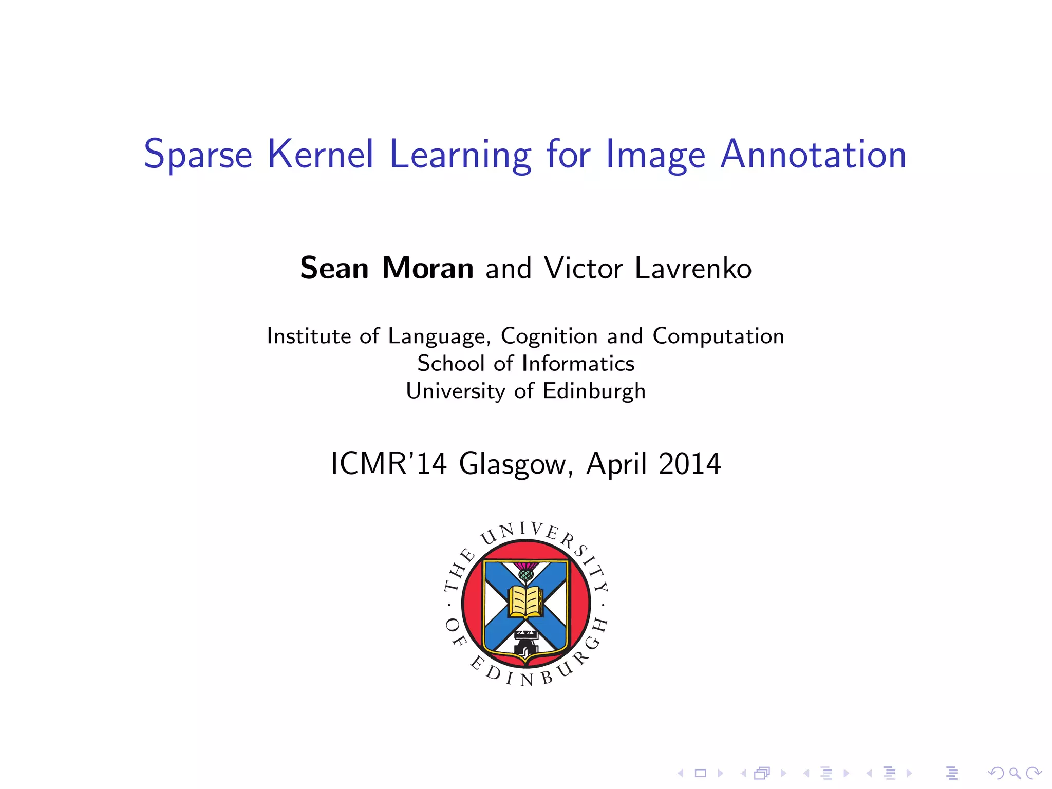
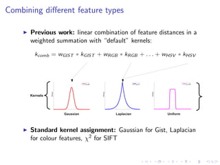
![Evaluation Metrics
Standard evaluation metrics [Guillaumin et al. ’09]:
Mean per word Recall (R)
Mean per word Precision (P)
F1 Measure
Number of words with recall > 0 (N+)
Fixed annotation length of 5 keywords](https://image.slidesharecdn.com/sklcrmtalk-140403051314-phpapp02/85/Sparse-Kernel-Learning-for-Image-Annotation-24-320.jpg)
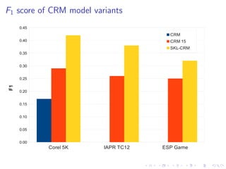
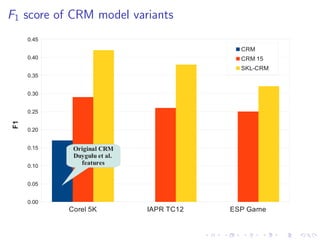
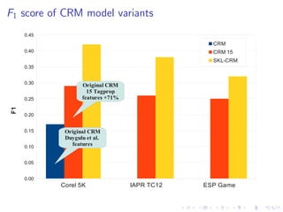
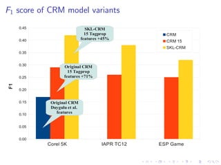
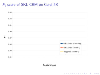
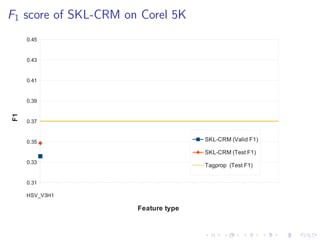
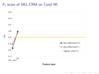
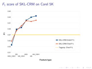
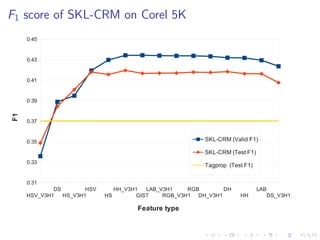
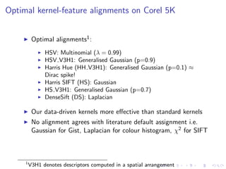
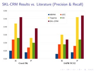
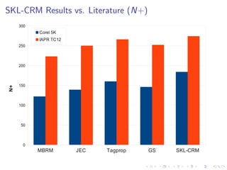
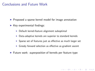

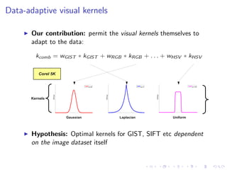
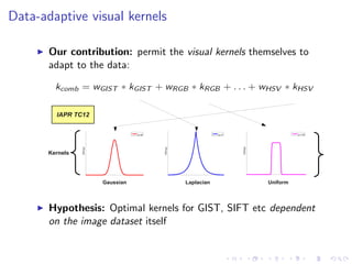
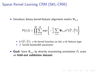
The document describes an approach called Sparse Kernel Continuous Relevance Model (SKL-CRM) for image annotation. SKL-CRM learns data-adaptive visual kernels to better combine different image features like GIST, SIFT, color, and texture. It introduces a binary kernel-feature alignment matrix to learn which kernel functions are best suited to which features by directly optimizing annotation performance on a validation set. Evaluation on standard datasets shows SKL-CRM improves over baselines with fixed 'default' kernels, achieving a relative gain of 10-15% in F1 score.