Downloaded 44 times


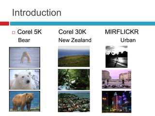
![Methodology
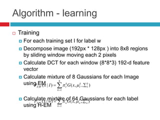
Mixture hierarchies
First step, get GMM from images – regular soft
EM
E:
M:
8
1
| ),,()|(
k
k
I
k
I
k
IWX xGIxP
Initialization
Euclidian distance
Mahalonobis
distance
Initial Par.
estimate
Expectation
Maximizaiton
Max iter. 200Change in likelihood
is too small
n
i
j jjiji xGjzzxP
1
2
1
),;()()|,(
)|,()|,()|,( 1 ttt
zxPzxPzxP
)],;([log),( ,|
ZXFEQ t
xz
t
),(maxarg1 tt
Q ](https://image.slidesharecdn.com/tencerpresentation-120413151853-phpapp02/85/Supervised-Learning-of-Semantic-Classes-for-Image-Annotation-and-Retrieval-9-320.jpg)
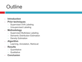
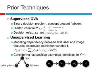
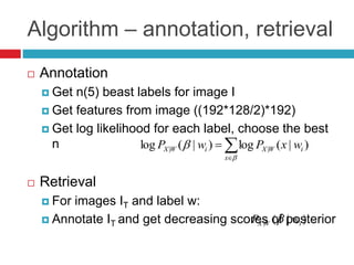
![Methodology
Mixture hierarchies for label
Second step, get HGMM for labels
E:
M:
64
1
| ),,()|(
k
k
w
k
w
k
wWX xGwxP Initialization
Bhattacharyya
distance
Initial Par.
estimate
Expectation
Maximizaiton
Max iter. 200Change in likelihood
is too small
n
i
j jjiji xGjzzxP
1
2
1
),;()()|,(
)|,()|,()|,( 1 ttt
zxPzxPzxP
)],;([log),( ,|
ZXFEQ t
xz
t
),(maxarg1 tt
Q ](https://image.slidesharecdn.com/tencerpresentation-120413151853-phpapp02/85/Supervised-Learning-of-Semantic-Classes-for-Image-Annotation-and-Retrieval-10-320.jpg)
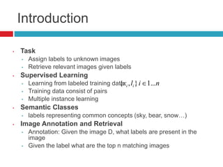
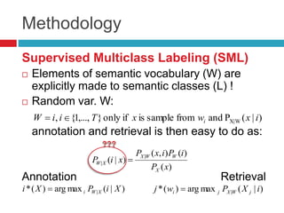
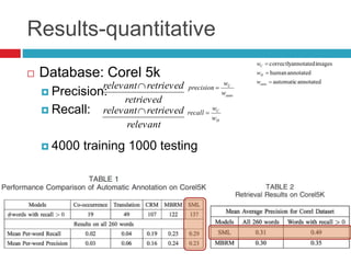
![E and M step for HGMM
Input:
Output:
E-step:
M-step:
KkDj i
k
j
k
j
k
j ,...,1,,...,1},,,{
l
l
c
Ntrace
l
c
l
c
k
j
m
c
Ntrace
m
c
m
c
k
jm
jk
k
j
k
j
l
c
k
j
k
j
m
c
eG
eG
h
]),,([
]),,([
}){(
2
1
}){(
2
1
1
1
Mmm
j
m
j
m
j ,...,1},,,{
KD
h
i
m
jkjknewm
c
)(
jk
jk
k
j
m
jk
k
j
m
jkm
jk
k
j
m
jk
newm
c
h
h
ww
where,)(
jk
Tm
c
k
j
m
c
k
j
k
j
m
jk
newm
c w ]))(([)( ](https://image.slidesharecdn.com/tencerpresentation-120413151853-phpapp02/85/Supervised-Learning-of-Semantic-Classes-for-Image-Annotation-and-Retrieval-11-320.jpg)
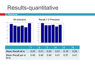
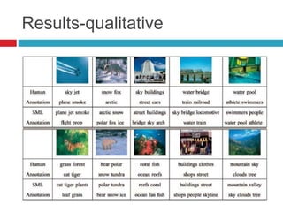
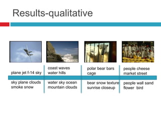
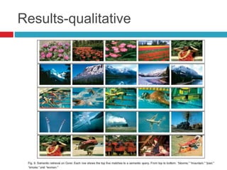


This document discusses methodologies for image annotation and retrieval using supervised and unsupervised learning techniques. It covers the estimation of semantic class distributions, image segmentation, and the performance evaluation through quantitative and qualitative results. The conclusions highlight the advantages and disadvantages of the proposed methods, including their effectiveness with weakly annotated data and the challenges of parameter tuning.


![[MIRU2018] Global Average Poolingの特性を用いたAttention Branch Network](https://cdn.slidesharecdn.com/ss_thumbnails/miru2018longorl-v3-180810062528-thumbnail.jpg?width=640&height=640&fit=bounds)


![[ppt]](https://cdn.slidesharecdn.com/ss_thumbnails/ppt2931-thumbnail.jpg?width=640&height=640&fit=bounds)
![[ppt]](https://cdn.slidesharecdn.com/ss_thumbnails/ppt3441-thumbnail.jpg?width=640&height=640&fit=bounds)