


![17
References
[1] PricewaterhouseCoopers LLP, PwC 2016
Global Industry 4.0 Survey - What we mean by
Industry 4.0 / Survey key findings / Blueprint
for digital success.
[2] “Is scheduling a solved problem?” - Stephen
F. Smith, Carnegie Mellon University, 5000
Forbes Avenue, Pittsburgh PA 15213 USA.
sfs@cs.cmu.edu.
[3] M. L. Pinedo. Scheduling: Theory,
Algorithms, and Systems. Springer, 4th edition,
2012. p. 431.
[4] Cowling, P.; Johansson, M. - Production,
Manufacturing and Logistics
Using real time information for effective
dynamic scheduling - Elsevier: European
Journal of Operational Research 139 (2002)
230–244](https://image.slidesharecdn.com/solvingschedulingproblem-170115114914/85/Solving-the-real-life-scheduling-problem-19-320.jpg)

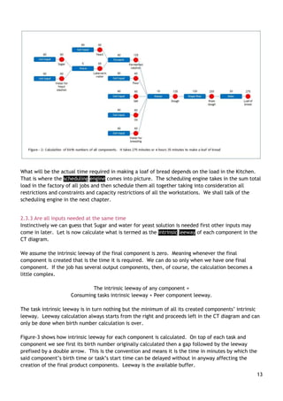
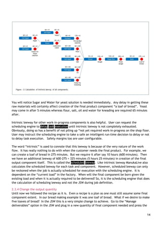
The document discusses a new method for solving the complex real-life scheduling problem in manufacturing processes, highlighting the challenges and failures of existing scheduling solutions. It introduces a Component Task Diagram (CT diagram) to represent and manage tasks and workstations effectively, integrating real-time feedback and rescheduling capabilities. The author emphasizes the importance of accurate scheduling for operational efficiency and invites readers to evaluate the proposed solution through available software downloads.


![Getting Started with Apache Spark: Big Data Made Simple [Free Meetup]](https://cdn.slidesharecdn.com/ss_thumbnails/apachesparkgettingstarted-260203175547-8361bcc3-thumbnail.jpg?width=640&height=640&fit=bounds)


