Download to read offline
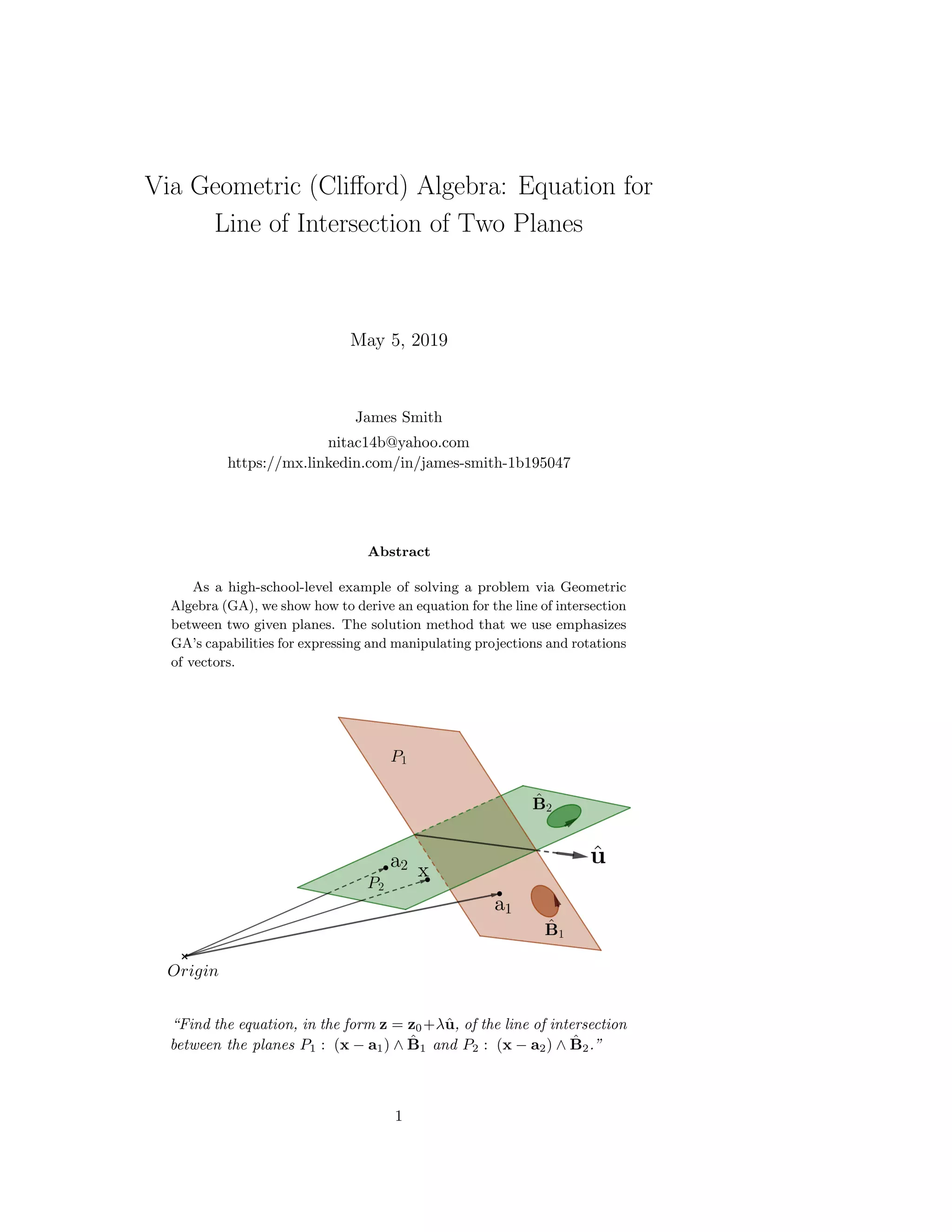
![Figure 1: Plane P1 consists of the endpoints of all those vectors x that satisfy
the condition expressed by the equation (x − a1) ∧ ˆB1 = 0. Plane P2 consists of
the endpoints of all those vectors x that satisfy the condition expressed by the
equation (x − a2) ∧ ˆB2 = 0.
1 Introduction
The line of intersection of two planes is an important element of many mathe-
matical and physical problems. Here, we’ll develop an equation for such a line
using Geometric-Algebra (GA) concepts that are discussed in greater detail in
Refs. [1] and [2].
2 Problem Statement
In Fig. 1,‘Given the planes (x − a1)∧ ˆB1 = 0 and (x − a2)∧ ˆB2 = 0,
derive an equation for their line of intersection, in the parametric
form z = z0 + λˆu.
3 Solution
To define the line of intersection, we will find the line’s direction (ˆu) and one
point along the line. As that point, we will choose the one closest to the origin.
We will call the vector from the origin to that point z0.](https://image.slidesharecdn.com/lineofintersection2planes-190505220546/75/Via-Geometric-Clifford-Algebra-Equation-for-Line-of-Intersection-of-Two-Planes-2-2048.jpg)
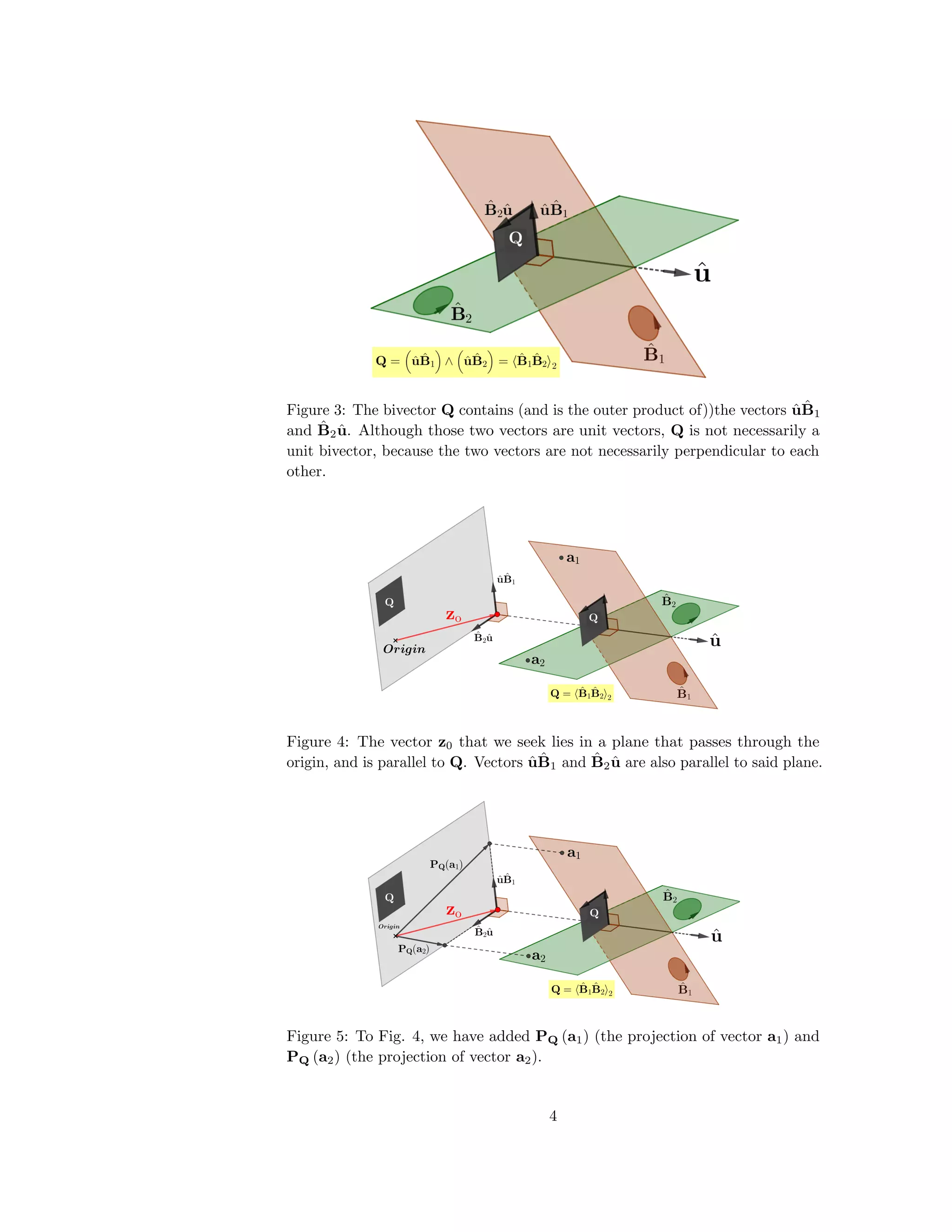
![Figure 6: Looking downward (i.e., in the direction −ˆu) upon the gray plane
shown in Figs. 4 and 5. To find z0, we will begin by solving the blue triangle
for the vector µ1 ˆu ˆB1. Then, z0 = PQ (a1) + µ1 ˆu ˆB1.
From Fig. 6,
µ1 ˆu ˆB1 + µ2
ˆB2 ˆu = PQ (a2) − PQ (a1) .
To solve for µ1, we’ll eliminate µ2 by taking the outer product of both sides
with the vector ˆB2 ˆu:
µ1 ˆu ˆB1 + µ2
ˆB2 ˆu ∧ ˆB2 ˆu = [PQ (a2) − PQ (a1)] ∧ ˆB2 ˆu
µ1 ˆu ˆB1 ∧ ˆB2 ˆu = [PQ (a2) − PQ (a1)] ∧ ˆB2 ˆu .
ˆQ
−1
= ˆQ, and ˆB1
ˆB2
−1
2 =
− ˆB1
ˆB2 2/ ˆB1
ˆB2 2
2
/
Next, we use properties of projections and the outer product to solve for µ1:
µ1 ˆu ˆB1
ˆB2 ˆu 2 = [PQ (a2 − a1)] ∧ ˆB2 ˆu
µ1
ˆB1
ˆB2 2 = (a2 − a1) · ˆQ ˆQ
−1
=PQ(a2−a1)
ˆB2 ˆu 2
µ1
ˆB1
ˆB2 2 = − (a2 − a1) · ˆQ ˆQ ˆB2 ˆu 2
µ1
ˆB1
ˆB2 2
ˆB1
ˆB2
−1
2 = (a2 − a1) · ˆQ ˆQ ˆB2 ˆu 2
ˆB1
ˆB2 2 / ˆB1
ˆB2 2
2
µ1 = (a2 − a1) ˆQ 1
=(a2−a1)· ˆQ
ˆQ ˆB2 ˆu 2
ˆB1
ˆB2 2 / ˆB1
ˆB2 2
2
= (a2 − a1) ˆQ 1
ˆQ −ˆu ˆB2 2
ˆB1
ˆB2 2 / ˆB1
ˆB2 2
2
= (a2 − a1) ˆQ 1 − ˆQˆu ˆB2 2
ˆB1
ˆB2 2 / ˆB1
ˆB2 2
2
.
5](https://image.slidesharecdn.com/lineofintersection2planes-190505220546/75/Via-Geometric-Clifford-Algebra-Equation-for-Line-of-Intersection-of-Two-Planes-5-2048.jpg)
![Now, we recall that ˆu = ˆQI−1
3 . Therefore, − ˆQˆu = − ˆQ ˆQI−1
3 = I−1
3 , and
µ1 = (a2 − a1) ˆQ 1I−1
3
ˆB2 2
ˆB1
ˆB2 2/ ˆB1
ˆB2 2
2
. (3.2)
Our purpose in finding µ1 was to then proceed to find µ1 ˆu ˆB1. We’ll do
that now.
µ1 ˆu ˆB1 =
(a2 − a1) ˆQ 1I−1
3
ˆB2 2
ˆB1
ˆB2 2
2
ˆB1
ˆB2 2
=µ1
ˆB1
ˆB2 2
ˆB1
ˆB2 2
I−1
3
=ˆu
ˆB1
= − (a2 − a1) ˆQ 1I−1
3
ˆB2 2I−1
3
ˆB1 / ˆB1
ˆB2 2 .
To finish, we recognize that I−1
3 = −I3, so that
µ1 ˆu ˆB1 = − (a2 − a1) ˆQ 1I3
ˆB2 2I3
ˆB1 / ˆB1
ˆB2 2 .
Then,
z0 = PQ (a2 − gabolda1) + µ1 ˆu ˆB1
= − (a2 − a1) ˆQ 1
ˆQ −
(a2 − a1) ˆQ 1I3
ˆB2 2I3
ˆB1
ˆB1
ˆB2 2
. (3.3)
References
[1] A. Macdonald, Linear and Geometric Algebra (First Edition) p. 126,
CreateSpace Independent Publishing Platform (Lexington, 2012).
[2] J. Smith, 2016, “Some Solution Strategies for Equations that Arise in
Geometric (Clifford) Algebra”, http://vixra.org/abs/1610.0054.
6](https://image.slidesharecdn.com/lineofintersection2planes-190505220546/75/Via-Geometric-Clifford-Algebra-Equation-for-Line-of-Intersection-of-Two-Planes-6-2048.jpg)

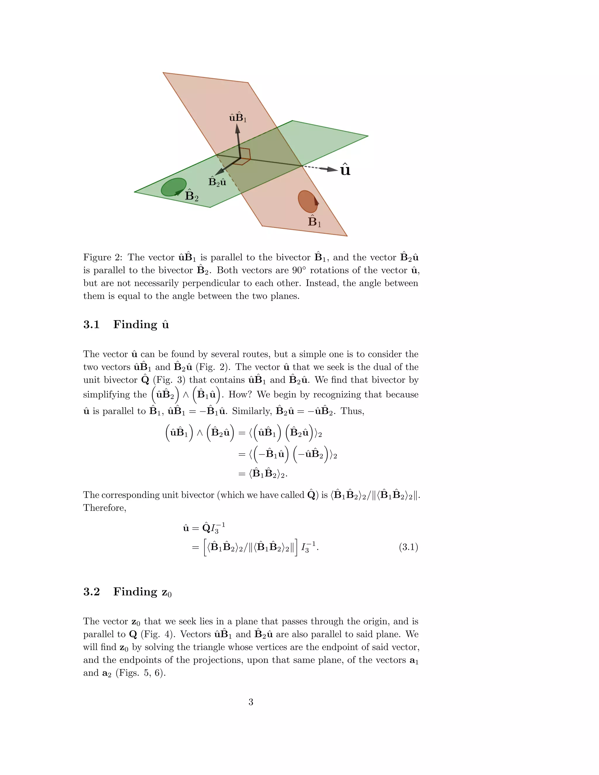
This document presents a method to derive the equation for the line of intersection of two planes using geometric algebra. It describes the steps to find the direction vector and a point on the line through a detailed problem-solving approach. The author illustrates the concepts with geometric interpretations and equations, enhancing understanding of geometric algebra's applications.


