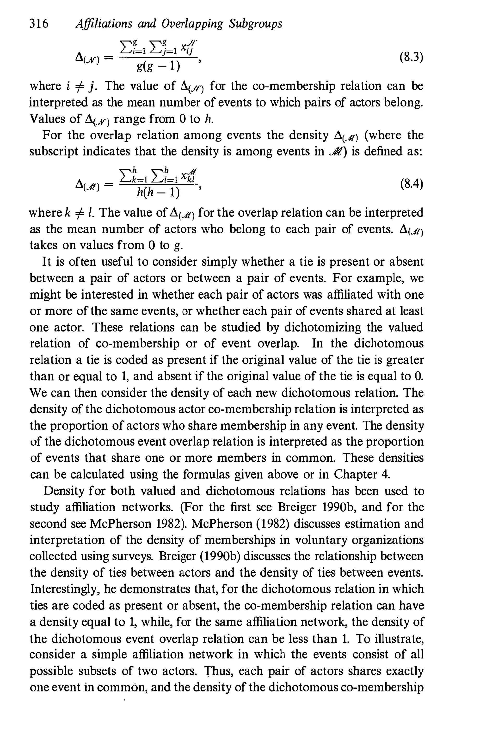
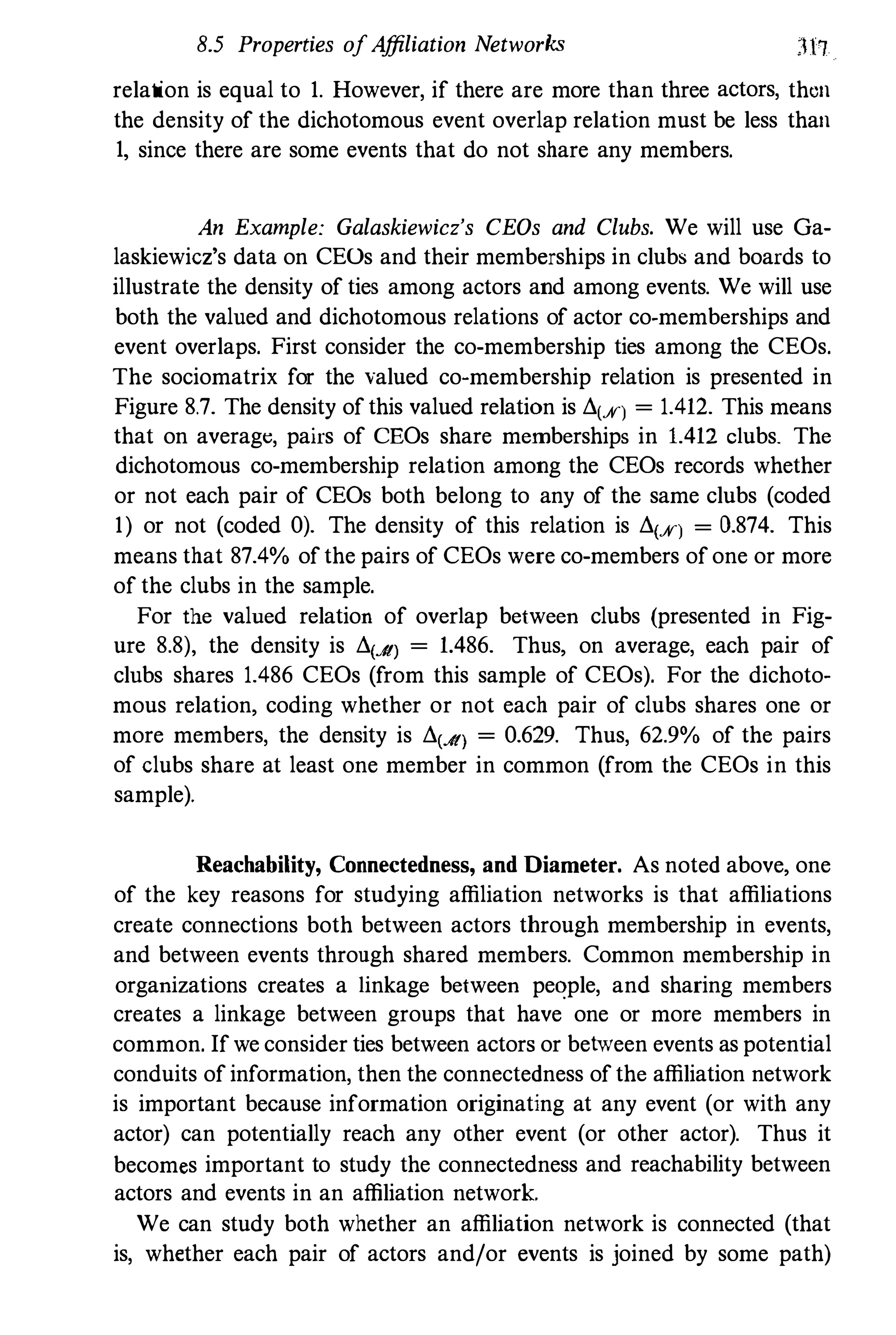
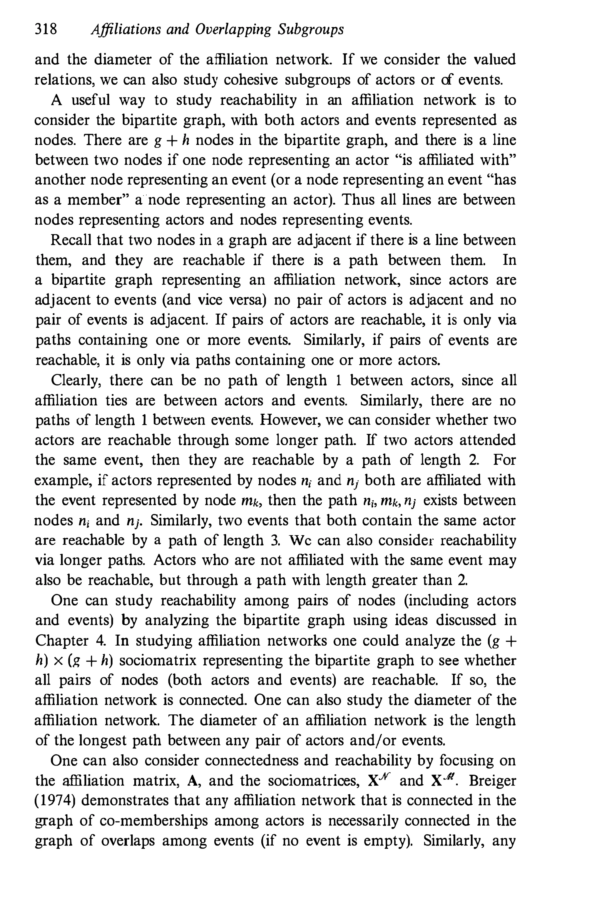
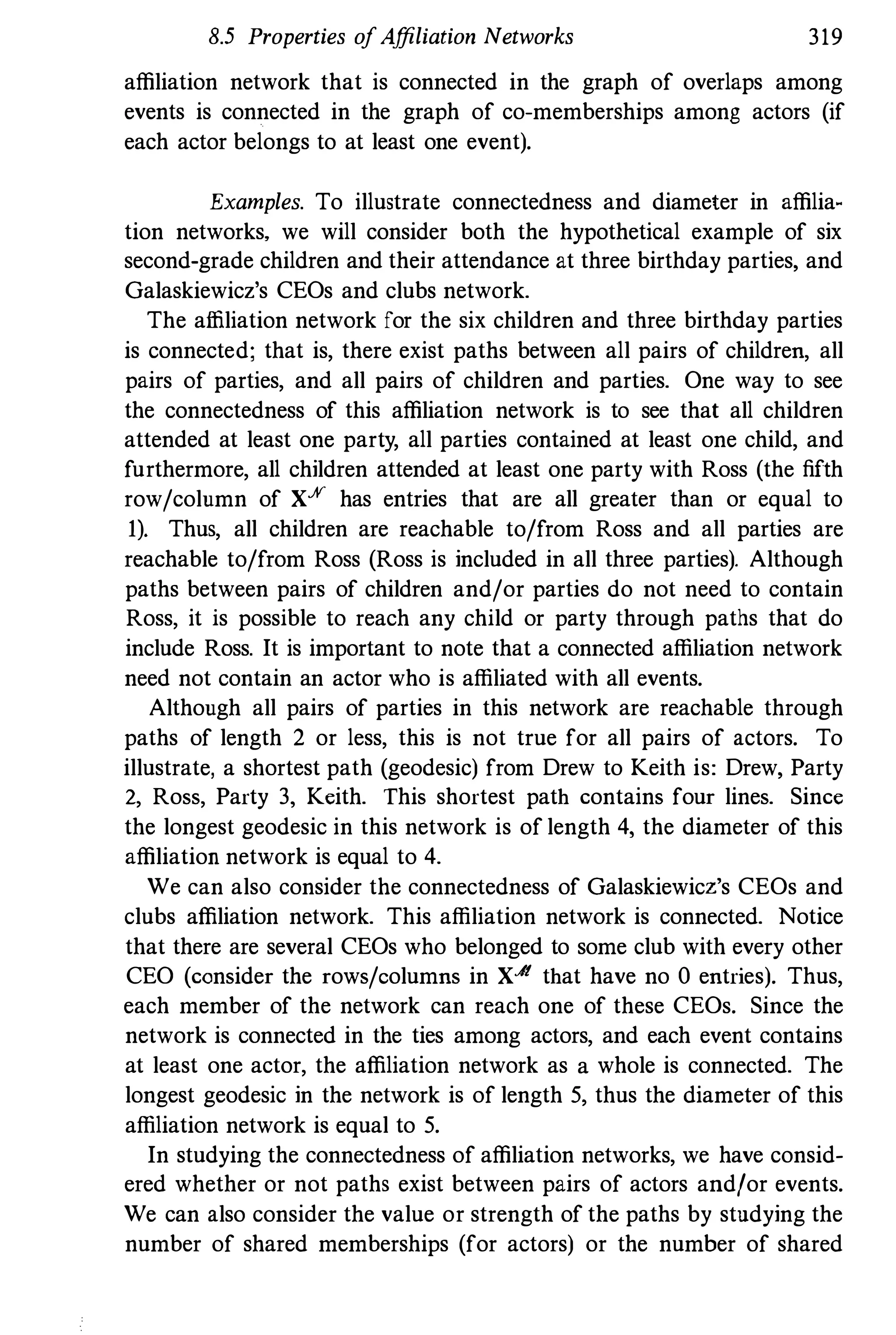
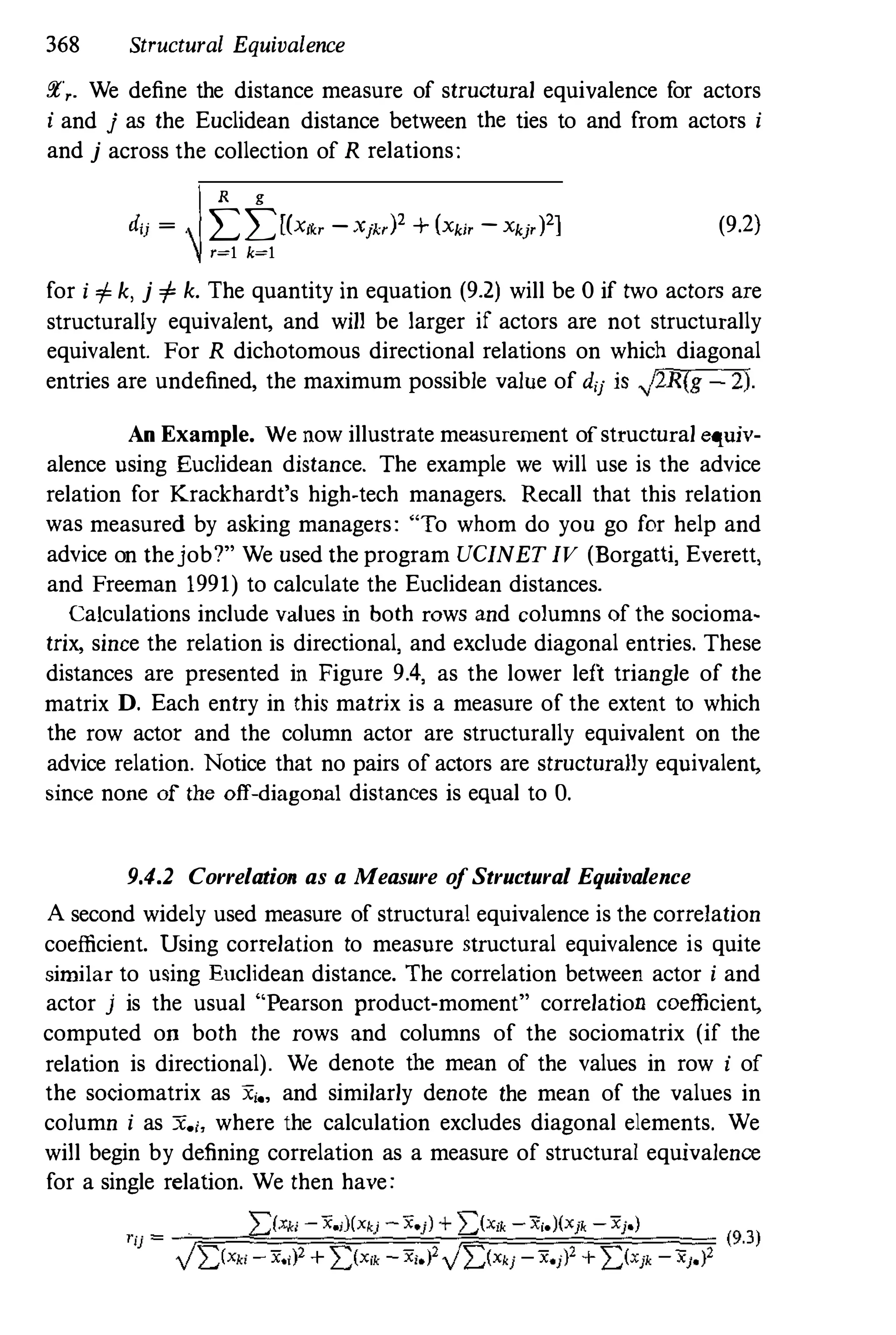
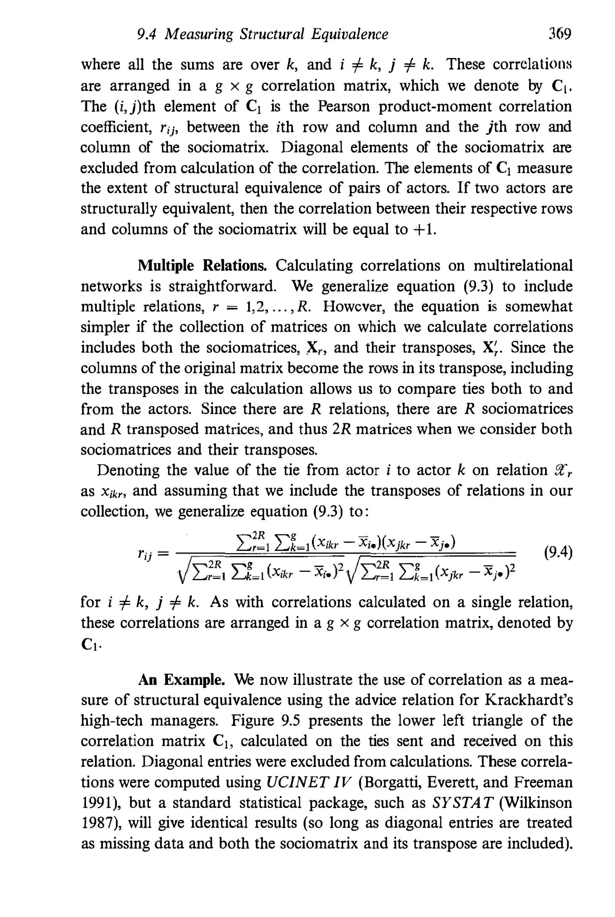
Social network analysis is used widely in the social and
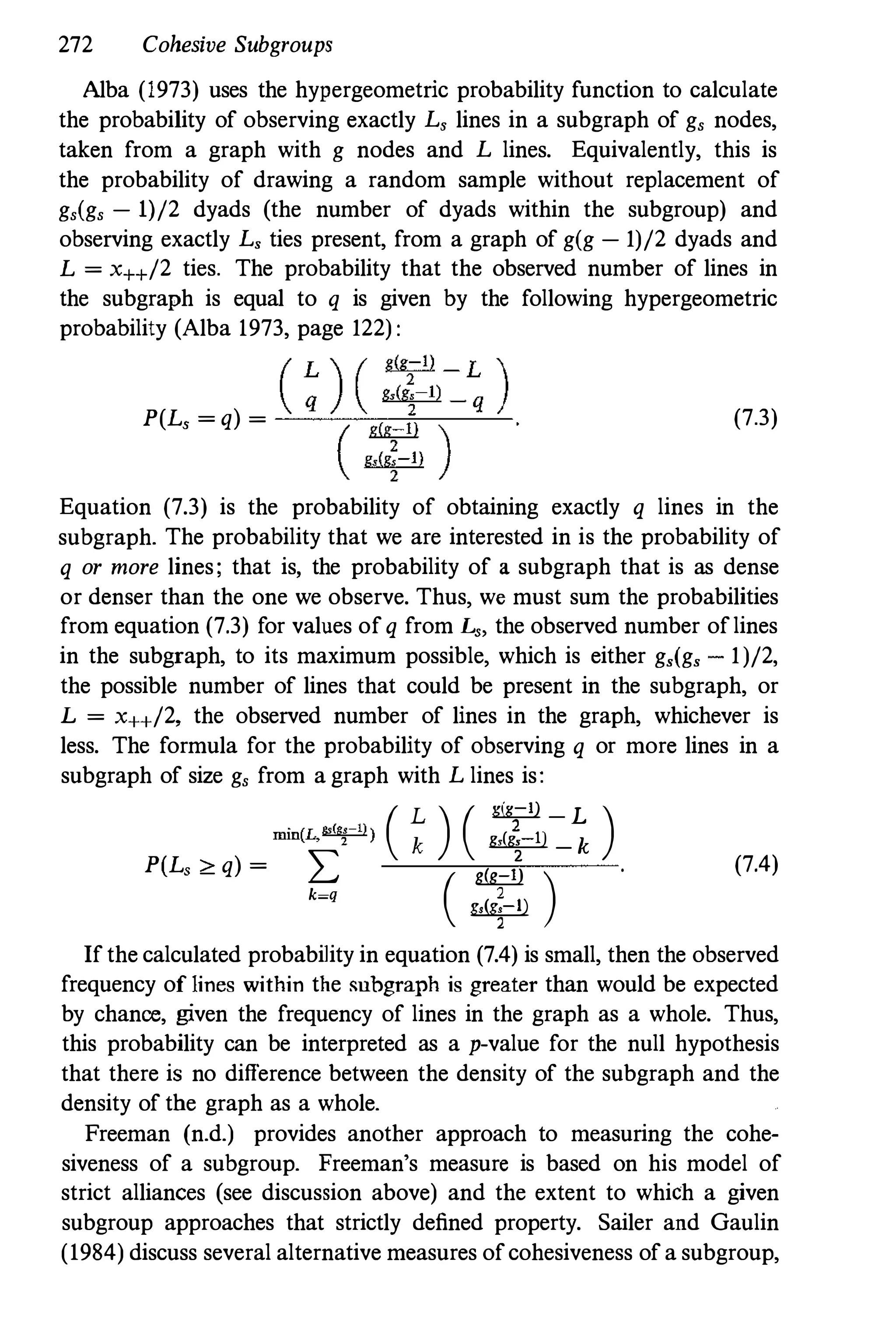
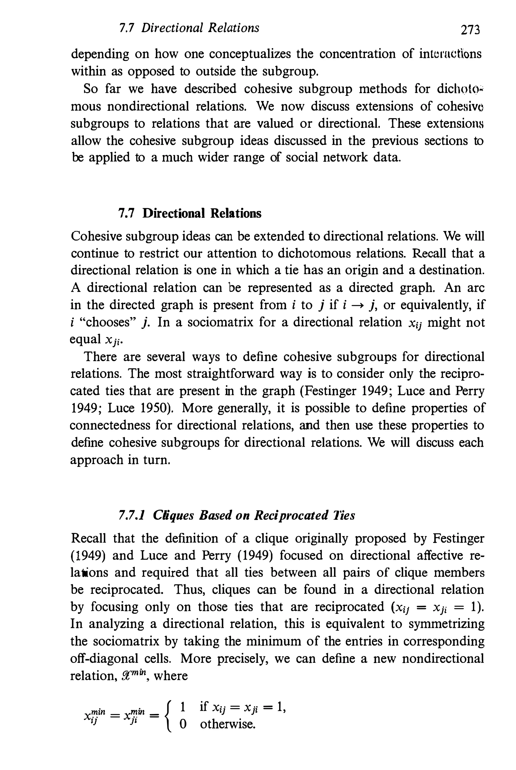
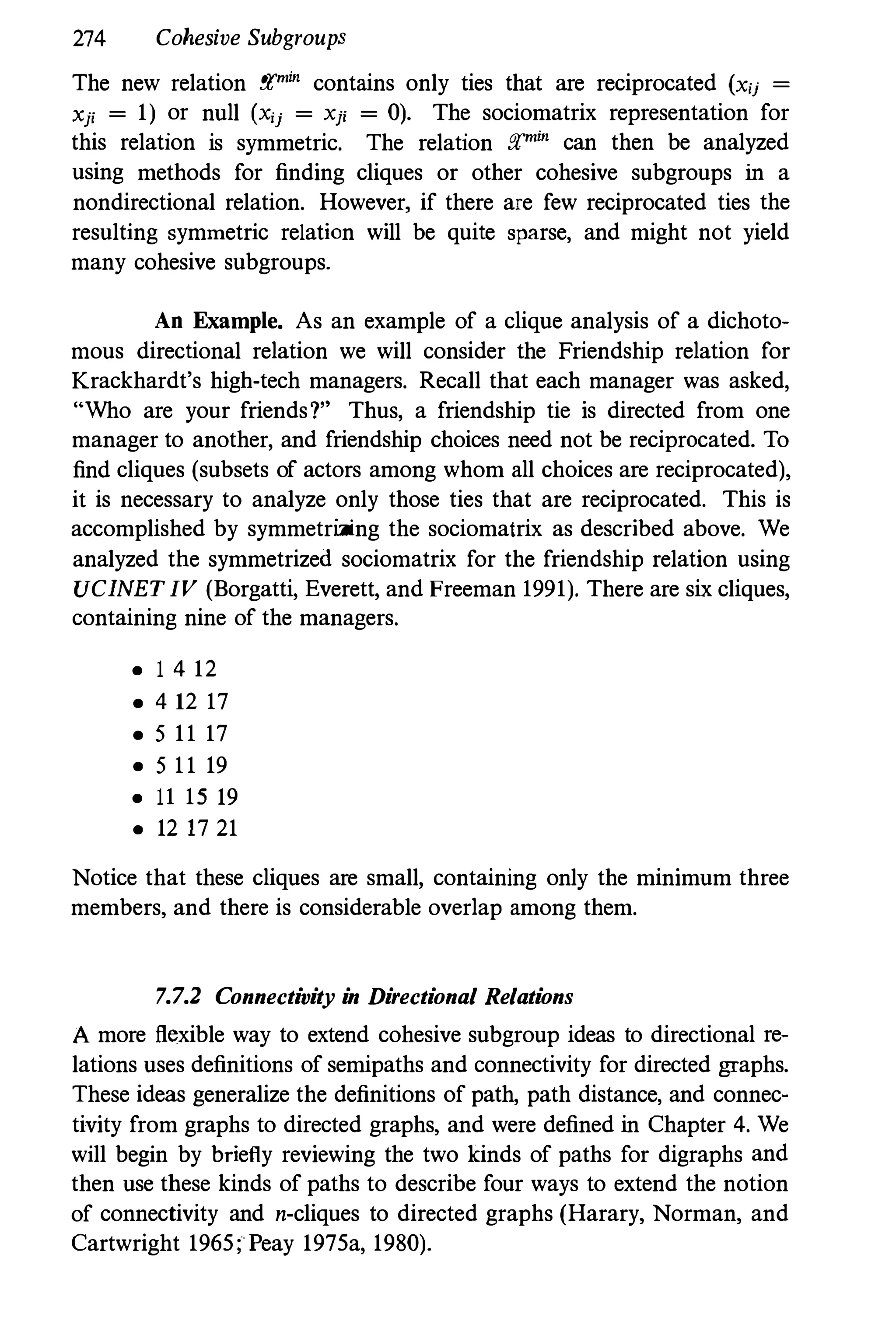
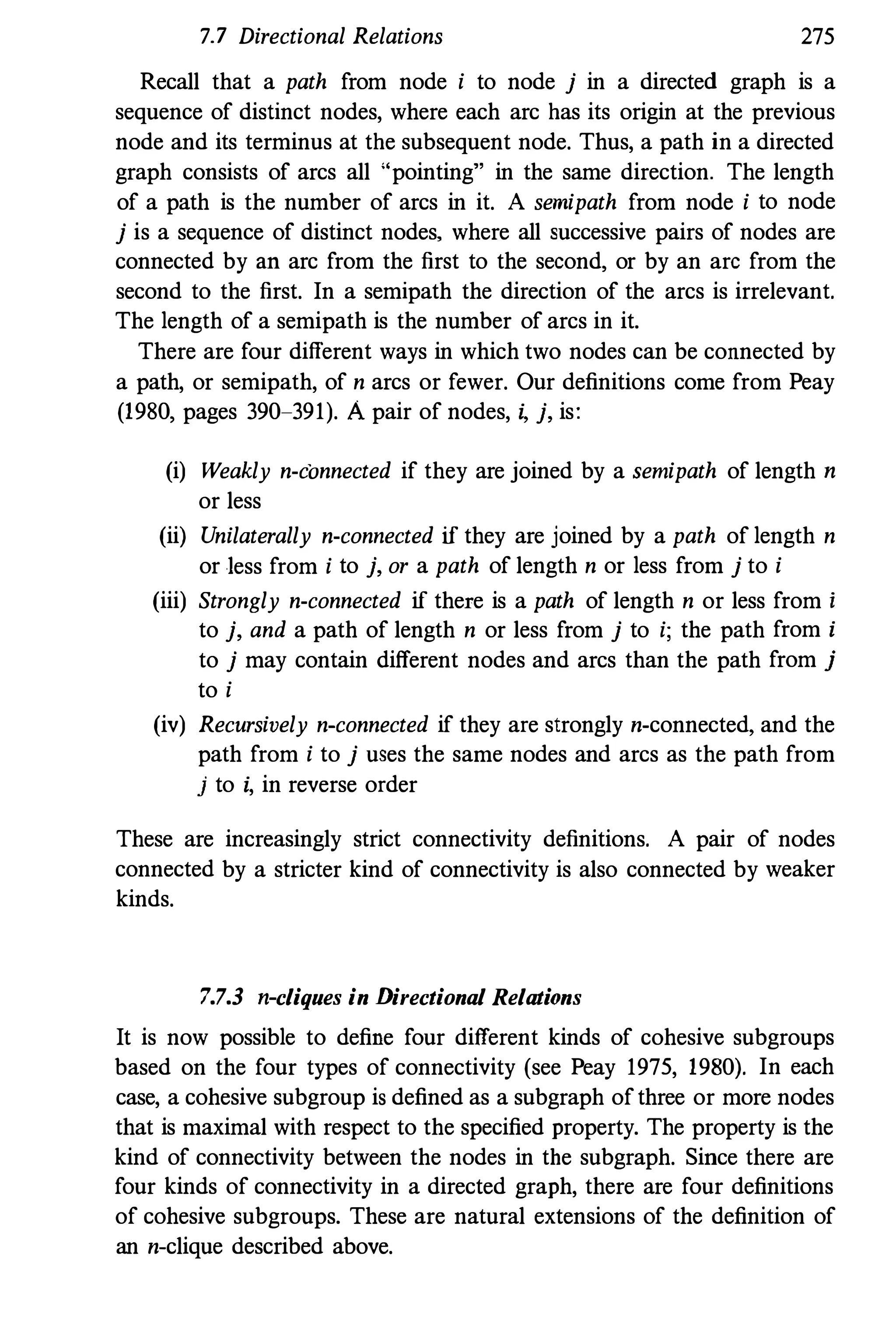
behavioral sciences, as well as in economics, marketing,and
industrial engineering. The social'network perspective focuses
on relationships among social entities; examples include
communications among members of a group, economic
transactions between corporations,and trade or treaties among
nations, The focus on relationships is an important addition to
standard social and behavioral research,which is primarily
concerned with attributes of the social units.
Social Network Analysis: Methods and Applications reviews and
discusses methods for the analysis of social networks with a
focus on applications of these methods to many substantive
examples. The book is organized into six parts. The
introductory chapters give an overview of the social network
perspective and describe different kinds of social network data.
The second part discusses formal representations for social
networks, including notations, graph theory, and matrix
operations. The third part covers structural and locational
properties of social networks, including centrality, prestige,
prominence, structural balance, clusterability, cohesive
subgroups, and affiliation networks. The fourth part examines
methods for social network roles and positions and includes
discussions of structural equivalence, blockmodels, and
relational algebras. The properties of dyads and triads are
covered in the fifth part of the book,and the final part
discusses statistical methods for social networks.
Social Network Analysis: Methods and Applications is a
reference book that can be used by those who want a
comprehensive review of network methods, or by researchers
who have gathered network data and want to find the most
appropriate method by which to analyze them. It is also
intended for use as a textbook,as it is the first book to provide
comprehensive coverage of the methodology and applications
of the field.
SOCIAL NETWORK ANALYSIS
Structural analysis in the social sciences
Mark Granovetter, editor
Other books in the series:
Ronald L. Breiger, ed., Social Mobility and Social Structure
John L. Campbell, J. Rogers Hollingsworth, and Leon N. Lindberg, eds.,
Governance ojthe American Economy
David Knoke, Political Networks: The Structural Perspective
Kyriakos Kontopoulos, The Logics oj Social Structure
Mark S. Mizruchi and Michael Schwartz, eds., Intercorporate Relations:
The Structural Analysis oj Business
Philippa Pattison, Algebraic Models jor Social Networks
Barry Wellman and S. D. Berkowitz, eds., Social Structures: A Network
Approach
The series Structural Analysis in the Social Sciences presents approaches
that explain social behavior and institutions by reference to relations
among such concrete entities as persons and organizations. This con­
trasts with at least four other popular strategies: (a) reductionist attempts
to explain by a focus on individuals alone; (b) explanations stressing the
causal primacy of such abstract concepts as ideas, values, mental har­
monies, and cognitive maps (thus, "structuralism" on the Continent
should be distinguished from structural analysis in the present sense);
(c) technological and material determinism; (d) explanations using "vari­
ables" as the main analytic concepts (as in the "structural equation"
models that dominated much of the sociology of the 1970s), where
structure is that connecting variables rather than actual social entities.
The social network approach is an important example of the strategy
of structural analysis; the series also draws on social science theory and
research that is not framed explicitly in network terms, but stresses the
importance of relations rather than the atomization of reductionism or
the determinism of ideas, technology, or material conditions. Though
the structural perspective has become extremely popular and influential
in all the social sciences, it does not have a coherent identity, and no
series yet pulls together such work under a single rubric. By bringing
the achievements of structurally oriented scholars to a wider public, the
Structural Analysis series hopes to encourage the use of this very fruitful
approach.
Mark Granovetter
SOCIAL NETWORK
ANALYSIS:
METHODS AND
APPLICATIONS
STANLEY WASSERMAN
University ofIllinols
KATHERINE FAUST
University ofSouth Carolina
CAMBRIDGE
UNIVERSITY PRESS
Published by the Press Syndicate of the University of Cambridge
The Pitt Building, Trumpington Street, Cambridge CB2 1RP
40 West 20th Street, New York, NY 10011-4211, USA
10 Stamford Road, Oakleigh, Melbourne 3166, Australia
© Cambridge University Press 1994
First published 1994
Printed in the United States of America
Library of Congress Cataloging-in-Publication Data
Wasserman, Stanley.
Social network analysis : methods and applications / Stanley
Wasserman, Katherine Faust.
p. crn. - (Structural analysis in the social sciences)
Includes bibliographical references and index.
ISBN 0-521-38269-6 (hacdback). - ISBN 0-521-38707-8 (pbk.)
L Social networks - Research - Methodology. 1. Faust, Katherine.
II. Title. III. Series.
HM13I.W356 1994
302'.01'1 - dc20 94-20602
A catalog record for this book is available from the British Library.
ISBN 0-521-38269-6 Hardback
ISBN 0-521-38707-8 Paperback
TAG
CIP
To Sarah
and
To Don and Margaret Faust
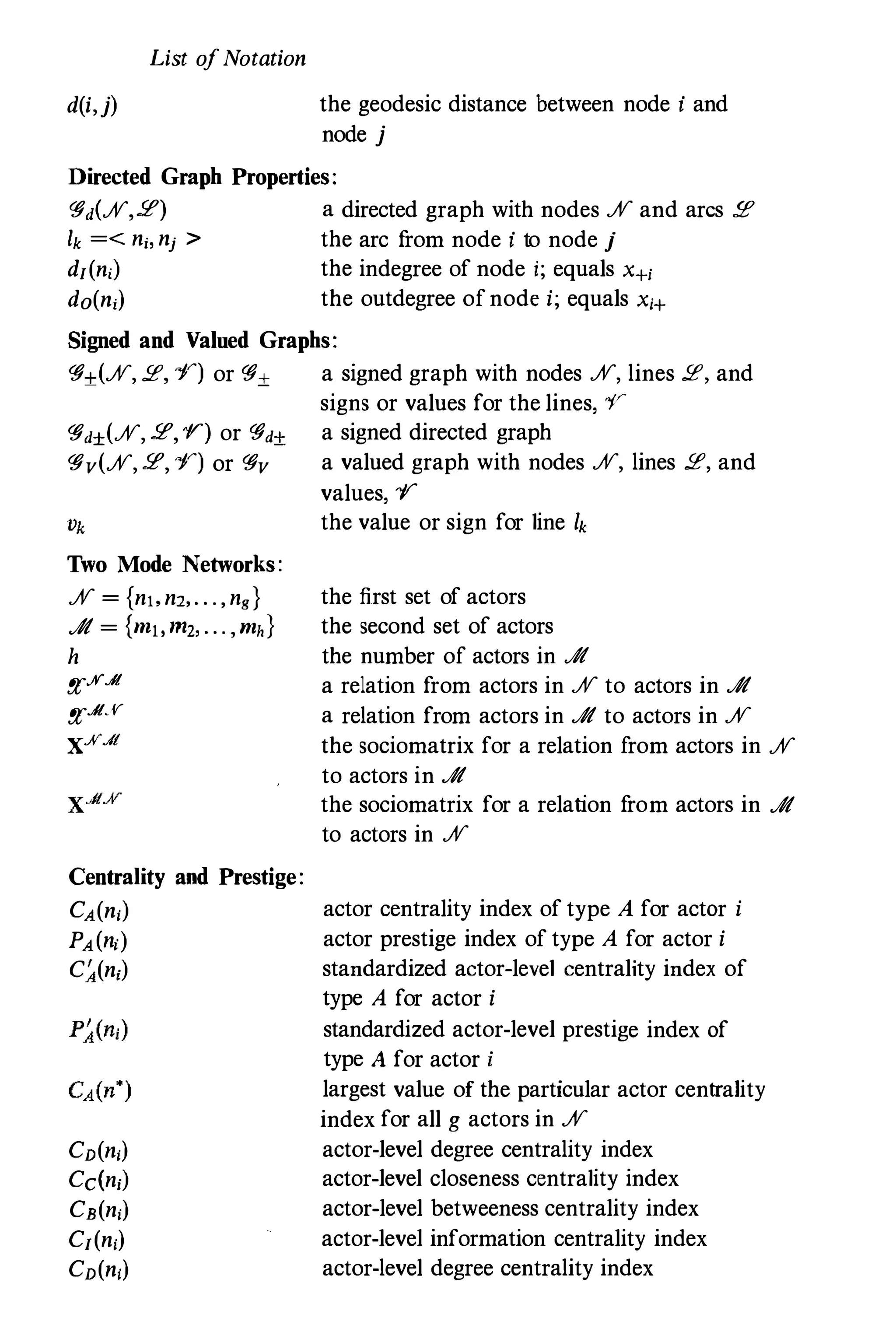
List of Notation
A Single Relation:
JV' = {nl,n2, ...,ng}
!!t
g
X
i--->j
I
XP
Multiple Relations:
R
!!t,
Sf,
L,
X,
Xijr
Graph Properties:
Sf = {h,12,... ,IL}
lk = (n;,nj)
L
<§(%, Sf)
d(n, )
11
the set of actors in a network or the set of
nodes in a graph
a single relation
the number of actors or nodes in %
the sociomatrix for relation !!t
elements of the sociomatrix X; value of the tie
from actor i to actor j
a tie from actor i to actor j
an incidence matrix
the pth power of a sociomatrix
the number of relations
the rth relation, r = 1,2,. .. ,R
the set of lines for the rth relation
the number oflines in Sf,
the sociomatrix for relation !!t,
elements of the sociomatrix X,
the set of lines
the line between nodes i and j
the number of lines in Sf
a graph consisting of node set % and line
set Sf
the degree of node i; d(n;) = x+, = x,+
the density of a graph
List ofNotation
d(i,j) the geodesic distance between node i and
node j
Directed Graph Properties:
�d(%,.P) a directed graph with nodes % and arcs.P
lk =< ni, nj > the arc from node i to node j
d,(n,) the indegree of node i; equals x+,
do(n,) the outdegree ofnode i; equals x,+
Signed and Valued Graphs:
�±(%,.P, 7'") or �± a signed graph with nodes %, lines .P, and
�d±(%,.P,"Y) or �d±
�v(%,.P,7'") or �v
Two Mode Networks:
% = {n!,n2,. . . ,ng}
.tr = {n1!,n12, . . . ,,"h}
h
;y;.KA
;y;A.K
X.K..I!
Centrality and Prestige:
CA(n,)
PA(n;)
C�(n,)
CD(n,)
Cdn,)
CB(n,)
C,(n,)
CD(n,)
signs or values for the lines, "Y
a signed directed graph
a valued graph with nodes %, lines .P, and
values, 7'"
the value or sign for line lk
the first set of actors
the second set of actors
the number of actors in .tr
a relation from actors in % to actors in .tr
a relation from actors in .tr to actors in %
the sociomatrix for a relation from actors in %
to actors in .tr
the sociomatrix for a relation from actors in .tr
to actors in %
actor centrality index of type A for actor i
actor prestige index of type A for actor i
standardized actor-level centrality index of
type A for actor i
standardized actor-level prestige index of
type A for actor i
largest value of the particular actor centrality
index for all g actors in %
actor-level degree centrality index
actor-level closeness centrality index
actor-level betweeness centrality index
actor-level information centrality index
actor-level degree centrality index
S2n
s'c
S21
Pn(n;)
Pp(n,)
PR(n,)
List ofNotation
Cohesive Subgroups:
cg,
.IV,
g,
fE,
d,(i)
A(i,j)
group-level centralization index of type A;
A = D,C,B,I
variance of the standardized degrees; index of
centralization
variance of the standardized closeness
centralities; index of centralization
variance of the standardized information
centralities; index of centralization
actor-level degree prestige index
actor-level proximity prestige index
actor-level rank prestige index
a subgraph
the set of nodes in subgraph cg,
the number of nodes in subgraph cg,
the set of lines in subgraph cg,
the degree of node i in subgraph cg,
the line connectivity of nodes i and j
Affiliations and Overlapping Subgroups:
ff=(d,@J) a hypergraph with point set d={a[,a2,...,ag},
x.J{ ={x;;1}
and edge set@J={Bj,B2,,,.,B.}
the sociomatrix for an affiliation network
sociomatrx of co-membership frequencies for
actors in .IV
sociomatrix of event overlap frequencies for
events in .4t
Structural Equivalence and Blockmodels:
!?4k an equivalence class or position
gk the number of actors in equivalence class k
B={bkl,} an image matrix for relation !Z',
B the number of positions (equivalence classes)
Ilkl' the density of block bkl,
d'j the Euclidean distance between sociomatrix
entries for actors i and j
the correlation between sociomatrix entries for
actors i and j
Relational Algebras:
List ofNotation
U, T, V,
iUj
o
ToU
i(TU)j
Positions and Roles:
<Po(i) = I'4Co)k
:i!BCEA)k
capital letters refer to relations
a tie from actor i to actor j on relation U
the operation of composition
the composition of relations T and U
a tie from actor i to actor j on the compound
relation TU
a set of distinct primitive and compound
relations
the role structure for a network with actor
set .AI'
the number of relations in Y
a partition (or reduction) of Y
the number of elements in fl
the joint homomorphic reduction of Y.¥ and
YJ/
the number of classes in fl�
the common structure semigroup for YJV and
[f'J/
the number of classes in fl��(
a measure of dissimilarity of role structures
YJV and YJ/ based on the joint
homomorphic reduction
a measure of similarity of role structures YJV
and Sf'dI based on hoth the joint homomorphic
reduction and the common structure
semigroup
assignment of actor i to equivalence class I'4Co)k
based on the equivalence definition "."
an equivalence class based on structural
equivalence
an equivalence class based on automorphic
equivalence
an equivalence class based on regular
equivalence
an equivalence class based on local role
equivalence
an equivalence class based on ego algebra
equivalence
List ofNotation
Mij
D(.9'-;,.'J'j)
oi}
Dyads and Reciprocity:
Dij = (Xij, Xj,)
{Dij}
< M,A,N >
Triads and Transitivity:
P-O-X
P-O-Q
+;­
PC;TC
a similarity measure of regular equivalence
a dissimilarity measure of role equivalence
a dissimilarity measure of ego algebra
equivalence
the dyad, or 2-subgraph, consisting of actors i
and j,for i i= j
collection of dyads
the dyad census; numbers of mutual,
asymmetric,and null dyads
indices of mutuality
two actors and an "object," about which
opinions are expressed
a triple of three actors; P and 0 have opinions
about Q
positive and negative signs for a line
the numbers of positive and total (semi)cycles
in a (di)graph
the triad, or 3-subgraph, involving ni, nj, and
nk, i < j < k
!T the set of all triads
T = {Tu;u = 1, 2, . .. ,16} the sixteen count triad census
I = (lu;u = 1,2,. . .,16) a linear combination vector of the triad census
PT
�T
Distributions:
P(.)
S
Gd(.;V)
U
Pi/= P(Xij = 1)
the mean of the triad census; the vector of
expected values of the Tu
the 16 x 16 covariance matrix of the triad
census
a test statistic to test specific configurations
derived from the triad census
test statistics for intransitivity and transitivity
the probability that the event "." occurs
the sample space of a random variable
the set of all possible directed graphs with g
nodes
the nniform random digraph distribution
the probability that a specific arc is present in
List ofNotation
B
UlMAN
PI and Relatives:
PI
y
w
w
Goodness-of-fit:
G2
!!.G2
dt; !!.dt
Obi
Ob2
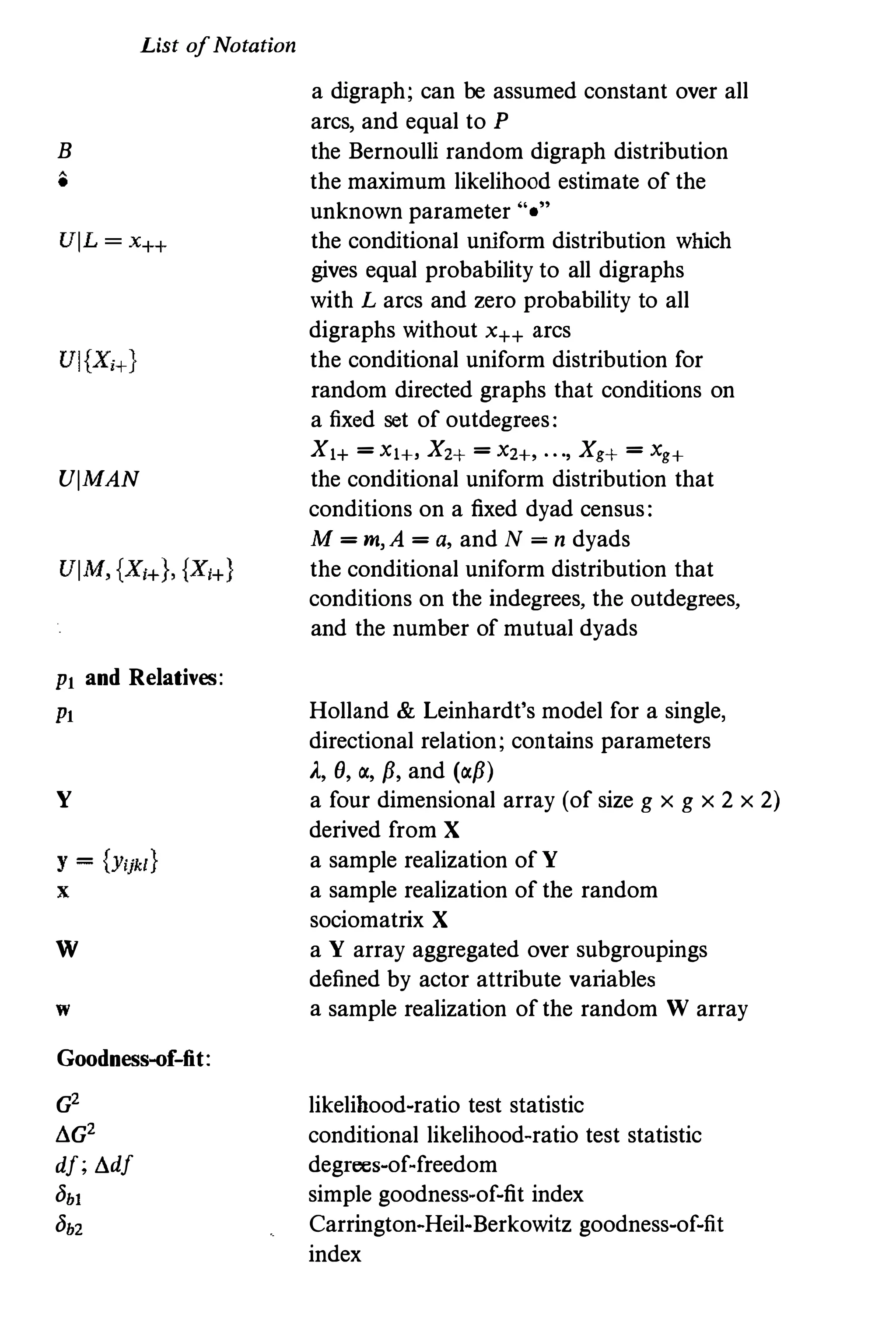
a digraph; can be assumed constant over all
arcs, and equal to P
the Bernoulli random digraph distribution
the maximum likelihood estimate of the
unknown parameter "."
the conditional uniform distribution which
gives equal probability to all digraphs
with L arcs and zero probability to all
digraphs without x++ arcs
the conditional uniform distribution for
random directed graphs that conditions on
a fixed set of outdegrees:
Xl+ = Xl+, X2+ = X2+, . . ., Xg+ = Xg+
the conditional uniform distribution that
conditions on a fixed dyad census:
M = m,A = a, and N = n dyads
the conditional uniform distribution that
conditions on the indegrees, the outdegrees,
and the number of mutual dyads
Holland & Leinhardt's model for a single,
directional relation; contains parameters
A, e, �, p,and (�p)
a four dimensional array (of size g x g x 2 x 2)
derived from X
a sample realization of Y
a sample realization of the random
sociomatrix X
a Y array aggregated over subgroupings
defined by actor attribute variables
a sample realization of the random W array
likelihood-ratio test statistic
conditional likelihood-ratio test statistic
degrees-of-freedom
simple goodness-of-fit index
Carrington-Heil-Berkowitz goodness-of-fit
index
List ofNotation
(t) - b
Xijr - ¢(i)¢(j)r
lix!
Stochastic Blockmodels:
X={xij,}
p(x)
Miscellaneous:
o
®
blockmodel predicted value
goodness-of-fit index comparing data to
predicted values
goodness-of-fit index; match coefficient
goodness-of-fit index; matrix correlation
super-sociomatrix of size g x g x r
the probability distribution for the
super-sociomatrix; also,a stochastic
blockmodel
a "tangential" section of the book
a "difficult" section of the book
Contents
List ofNotation
List of Tables
List ofIllustrations
Preface
Part I: Networks, Relations, and Structure
page xxi
XXIV
xxix
1
1 Social Network Analysis in the Social and Behavioral Sciences 3
1.1 The Social Networks Perspective 4
1.2 Historical and Theoretical Foundations 10
1.2.1 Empirical Motivations 11
1.2..2 Theoretical Motivations 13
1.2.3 Mathematical Motivations 15
1.2.4 In Summary 16
1.3 Fundamental Concepts in Network Analysis 17
1.4 Distinctive Features 21
1.5 Organization of the Book and How to Read It 22
1.5.1 Complexity 23
1.5.2 Descriptive and Statistical Methods 23
1.5.3 Theory Driven Methods 24
1.5.4 Chronology 24
1.5.5 Levels of Analysis 25
1.5.6 Chapter Prerequisites 26
1.6 Summary 27
2 Social Network Data 28
2.1 Introduction: What Are Network Data? 28
2.1.1 Structural and Composition Variables 29
ix
x Contents
2.1.2 Modes
2.1.3 Affiliation Variables
2.2 Boundary Specification and Sampling
2.2.1 What Is Your Population?
2.2.2 Sampling
2.3 Types of Networks
2.3.1 One-Mode Networks
2.3.2 Two-Mode Networks
2.3.3 Ego-centered and Special Dyadic Networks
2.4 Network Data, Measurement and Collection
2.4.1 Measurement
2.4.2 Collection
2.4.3 Longitudinal Data Collection
29
30
30
31
33
35
36
39
41
43
43
45
55
2.4.4 Measurement Validity, Reliability, Accuracy, Error 56
2.5 Data Sets Found in These Pages 59
2.5.1 Krackhardt's High-tech Managers 60
2.5.2 Padgett's Florentine Families 61
2.5.3 Freeman's EIES Network 62
2.5.4 Countries Trade Data 64
2.5.5 Galaskiewicz's CEOs and Clubs Network 65
2.5.6 Other Data 66
Part II: Mathematical Representations of Social Networks 67
3 Notation for Social Network Data 69
3.1 Graph Theoretic Notation 71
3.1.1 A Single Relation 71
3.1.2 OMultiple Relations 73
3.1.3 Summary 75
3.2 Sociometric Notation 77
3.2.1 Single Relation 79
3.2.2 Multiple Relations 81
3.2.3 Summary 83
3.3 OAlgebraic Notation 84
3.4 OTwo Sets of Actors 85
3.4.1 @Different Types ofPairs 86
3.4.2 OSociometric Notation 87
3.5 Putting It All Together 89
Contents xi
4 Graphs and Matrices 92
4.1 Why Graphs? 93
4.2 Graphs 94
4.2.1 Subgraphs, Dyads, and Triads 97
4.2.2 Nodal Degree 100
4.2.3 Density of Graphs and Suhgraphs 101
4.2.4 Example: Padgett's Florentine Families 103
4.2.5 Walks, Trails, and Paths 105
4.2.6 Connected Graphs and Components 109
4.2.7 Geodesics, Distance, and Diameter 110
4.2.8 Connectivity of Graphs 112
4.2.9 Isomorphic Graphs and Subgraphs 117
4.2.10 OSpecial Kinds of Graphs 119
4.3 Directed Graphs 121
4.3.1 Subgraphs - Dyads 124
4.3.2 Nodal Indegree and Qutdegree 125
4.3.3 Density of a Directed Graph 129
4.3.4 An Example 129
4.3.5 Directed Walks, Paths,Semipaths 129
4.3.6 Reachability and Connectivity in Digraphs 132
4.3.7 Geodesics, Distance and Diameter 134
4.3.8 OSpecial Kinds of Directed Graphs 134
4.3.9 Summary 136
4.4 Signed Graphs and Signed Directed Graphs 136
4.4.1 Signed Graph 137
4.4.2 Signed Directed Graphs 138
4.5 Valued Graphs and Valued Directed Graphs 140
4.5.1 Nodes and Dyads 142
4.5.2 Density in a Valued Graph 143
4.5.3 OPaths in Valued Graphs 143
4.6 Multigraphs 145
4.7 i8)Hypergraphs 146
4.8 Relations 148
4.8.1 Definition 148
4.8.2 Properties of Relations 149
4.9 Matrices 150
4.9.1 Matrices for Graphs 150
4.9.2 Matrices for Digraphs 152
4.9.3 Matrices for Valued Graphs 153
4.9.4 Matrices for Two-Mode Networks 154
xu Contents
4.9.5 OMatrices for Hypergraphs
4.9.6 Basic Matrix Operations
4.9.7 Computing Simple Network Properties
4.9.8 Summary
4.10 Properties
4.10.1 Reflexivity
4.10.2 Symmetry
4.10.3 Transitivity
4.11 Summary
Part III: Structural and Locational Properties
5 Centrality and Prestige
5.1 Prominence: Centrality and Prestige
5.1.1 Actor Centrality
5.1.2 Actor Prestige
5.1.3 Group Centralization and Group Prestige
5.2 Nondirectional Relations
5.2.1 Degree Centrality
5.2.2 Closeness Centrality
5.2.3 Betweenness Centrality
5.2.4 ®Information Centrality
5.3 Directional Relations
5.3.1 Centrality
5.3.2 Prestige
5.3.3 A Different Example
5.4 Comparisons and Extensions
6 Structural Balance and Transitivity
6.1 Structural Balance
6.1.1 Signed Nondirectional Relations
6.1.2 Signed Directional Relations
6.1.3 OChecking for Balance
6.1.4 An Index for Balance
6.1.5 Summary
6.2 Clusterability
6.2.1 The Clustering Theorems
6.2.2 Summary
6.3 Generalizations of Clusterability
154
154
159
164
164
164
165
165
165
167
169
172
173
174
175
177
178
183
188
192
198
199
202
210
215
220
222
223
228
230
232
232
233
235
238
239
Contents xiii
6.3.1 Empirical Evidence 239
6.3.2 ORanked Clusterability 240
6.3.3 Summary 242
6.4 Transitivity 243
6.5 Conclusion 247
7 Cohesive Subgroups 249
7.1 Backgrouud 250
7.1.1 Social Group and Subgroup 250
7.1.2 Notation 252
7.2 Subgroups Based on Complete Mutuality 253
7.2.1 Definition of a Clique 254
7.2.2 An Example 254
7.2.3 Considerations 256
7.3 Reachability and Diameter 257
7.3.1 n-cliques 258
7.3.2 An Example 259
7.3.3 Considerations 260
7.3.4 n-clans and n-clubs 260
7.3.5 Summary 262
7.4 Subgroups Based on Nodal Degree 263
7.4.1 k-plexes 265
7.4.2 k-cores 266
7.5 Comparing Within to Outside Subgroup Ties 267
7.5.1 LS Sets 268
7.5.2 Lambda Sets 269
7.6 Measures of Subgroup Cohesion 270
7.7 Directional Relations 273
7.7.1 Cliques Based on Reciprocated Ties 273
7.7.2 Connectivity in Directional Relations 274
7.7.3 n-cliques in Directional Relations 275
7.8 Valued Relations 277
7.8.1 Cliques,n-cliques,and k-plexes 278
7.8.2 Other Approaches for Valued Relations 282
7.9 Interpretation of Cohesive Subgroups 283
7.10 Other Approaches 284
7.10.1 Matrix Permutation Approaches 284
7.10.2 Multidimensional Scaling 287
7.10.3 OFactor Analysis 290
7.11 Summary 290
xiv Contents
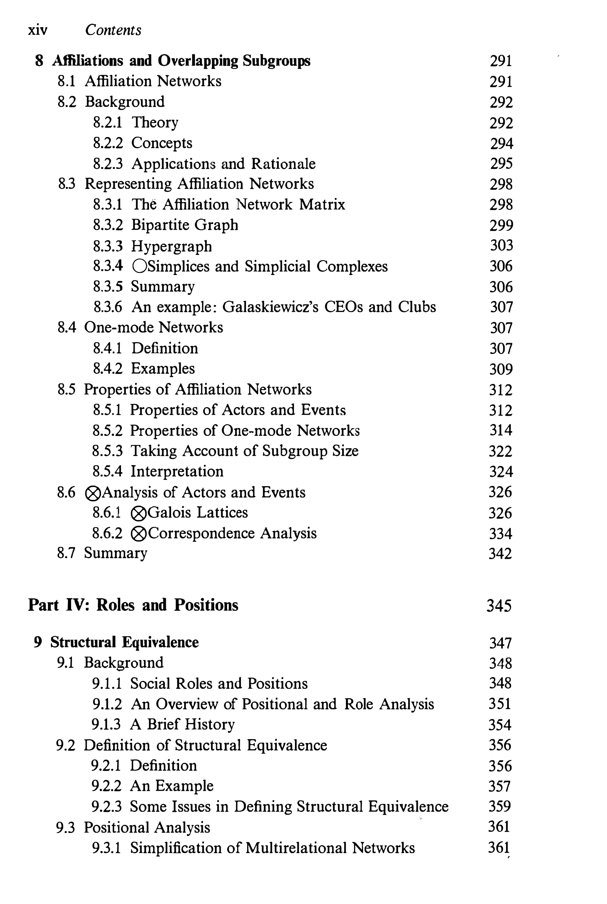
8 Affiliations and Overlapping Subgroups 291
8.1 Affiliation Networks 291
8.2 Background 292
8.2.1 Theory 292
8.2.2 Concepts 294
8.2.3 Applications and Rationale 295
8.3 Representing Affiliation Networks 298
8.3.1 The Affiliation Network Matrix 298
8.3.2 Bipartite Graph 299
8.3.3 Hypergraph 303
8.3.4 OSimplices and Simplicial Complexes 306
8.3.5 Summary 306
8.3.6 An example: Galaskiewicz's CEOs and Clubs 307
8.4 One-mode Networks 307
8.4.1 Definition 307
8.4.2 Examples 309
8.5 Properties of Affiliation Networks 312
8.5.1 Properties of Actors and Events 312
8.5.2 Properties of One-mode Networks 314
8.5.3 Taking Account of Subgroup Size 322
8.5.4 Interpretation 324
8.6 ®Analysis of Actors and Events 326
8.6.1 ®Galois Lattices 326
8.6.2 ®Correspondence Analysis 334
8.7 Summary 342
Part IV: Roles and Positions 345
9 Structural Equivalence 347
9.1 Background 348
9.1.1 Social Roles and Positions 348
9.1.2 An Overview of Positional and Role Analysis 351
9.1.3 A Brief History 354
9.2 Definition of Structnral Equivalence 356
9.2.1 Definition 356
9.2.2 An Example 357
9.2.3 Some Issues in Defining Structural Equivalence 359
9.3 Positional Analysis 361
9.3.1 Simplification of Multirelational Networks 361
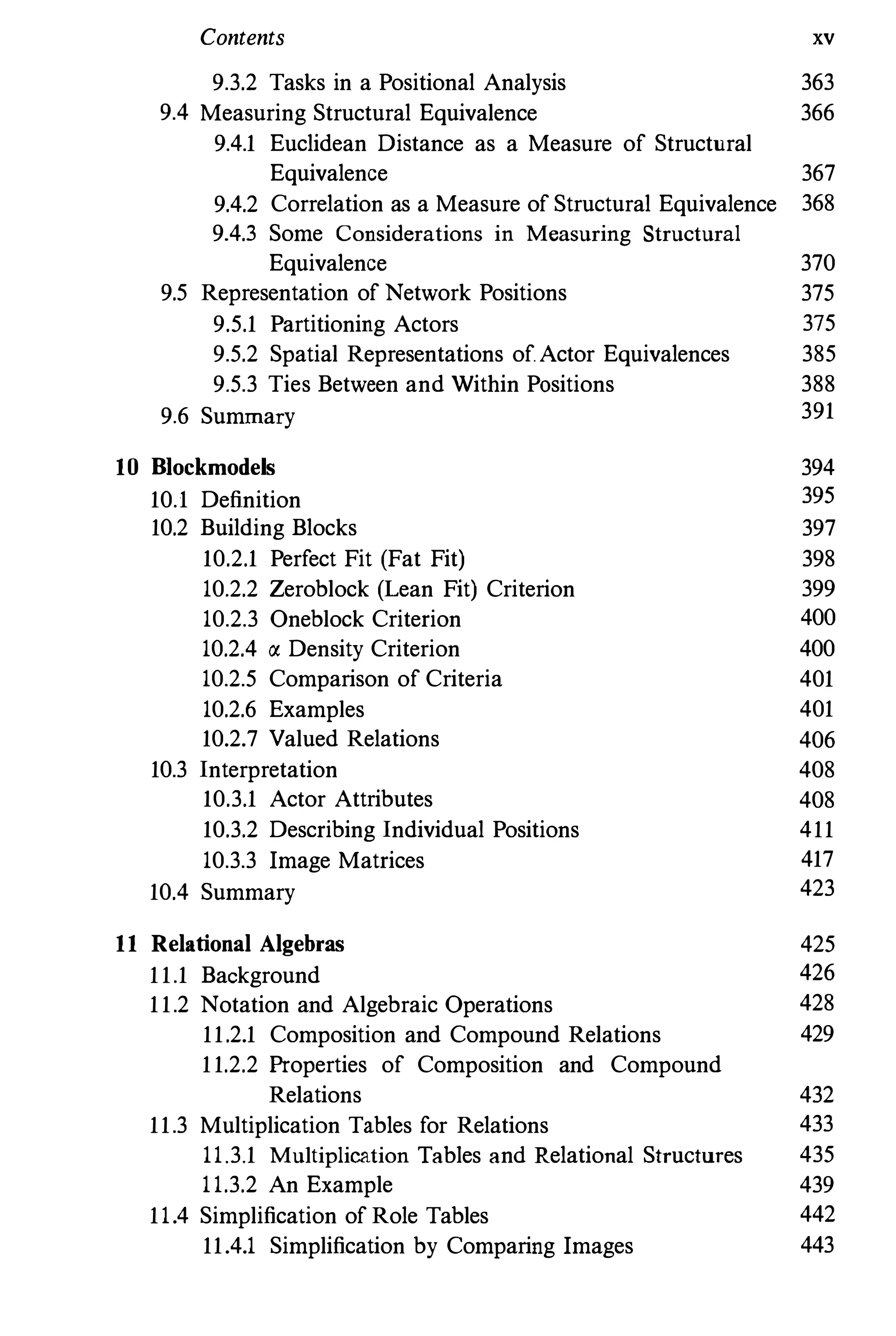
Contents xv
9.3.2 Tasks in a Positional Analysis 363
9.4 Measuring Structural Equivalence 366
9.4.1 Euclidean Distance as a Measure of Structural
Equivalence 367
9.4.2 Correlation as a Measure of Structural Equivalence 368
9.4.3 Some Considerations in Measuring Structural
Equivalence 370
9.5 Representation of Network Positions 375
9.5.1 Partitioning Actors 375
9.5.2 Spatial Representations of.Actor Equivalences 385
9.5.3 Ties Between and Within Positions 388
9.6 Summary 391
10 B1ockmodels 394
10.1 Definition 395
10.2 Building Blocks 397
10.2.1 Perfect Fit (Fat Fit) 398
10.2.2 Zeroblock (Lean Fit) Criterion 399
10.2.3 Oneblock Criterion 400
10.2.4 " Density Criterion 400
10.2.5 Comparison of Criteria 401
10.2.6 Examples 401
10.2.7 Valued Relations 406
10.3 Interpretation 408
10.3.1 Actor Attributes 408
10.3.2 Describing Individual Positions 411
10.3.3 Image Matrices 417
10.4 Summary 423
11 Relational Algebras 425
11.1 Background 426
11.2 Notation and Algebraic Operations 428
11.2.1 Composition and Compound Relations 429
11.2.2 Properties of Composition and Compound
Relations 432
11.3 Multiplication Tables for Relations 433
11.3.1 Multiplication Tables and Relational Structures 435
11.3.2 An Example 439
11.4 Simplification of Role Tables 442
11.4.1 Simplification by Comparing Images 443
XVI Contents
11.4.2 ®Homomorphic Reduction 445
11.5 ®Comparing Role Structures 449
11.5.1 Joint Homomorphic Reduction 451
11.5.2 The Common Structure Semigroup 452
11.5.3 An Example 453
11.5.4 Measuring the Similarity of Role Structures 457
11.6 Summary 460
12 Network Positions and Roles 461
12.1 Background 462
12.1.1 Theoretical Definitions of Roles and Positions 462
12.1.2 Levels of Role Analysis in Social Networks 464
12.1.3 Equivalences in Networks 466
12.2 Structural Equivalence, Revisited 468
12.3 Automorphic and Isomorphic Equivalence 469
12.3.1 Definition 470
12.3.2 Example 471
12.3.3 Measuring Automorphic Equivalence 472
12.4 Regular Equivalence 473
12.4.1 Definition of Regular Equivalence 474
12.4.2 Regular Equivalence for Nondirectional Relations 475
12.4.3 Regular Equivalence Blockmodels 476
12.4.4 OA Measure of Regular Equivalence 479
12.4.5 An Example 481
12.5 "Types" of Ties
12.5.1 An Example
12.6 Local Role Equivalence
12.6.1 Measuring Local Role Dissinrilarity
12.6.2 Examples
12.7 ®Ego Algebras
12.7.1 Definition of Ego Algebras
12.7.2 Equivalence of Ego Algebras
12.7.3 Measuring Ego Algebra Sintilarity
12.7.4 Examples
12.8 Discussion
483
485
487
488
491
494
496
497
497
499
502
Contents xvii
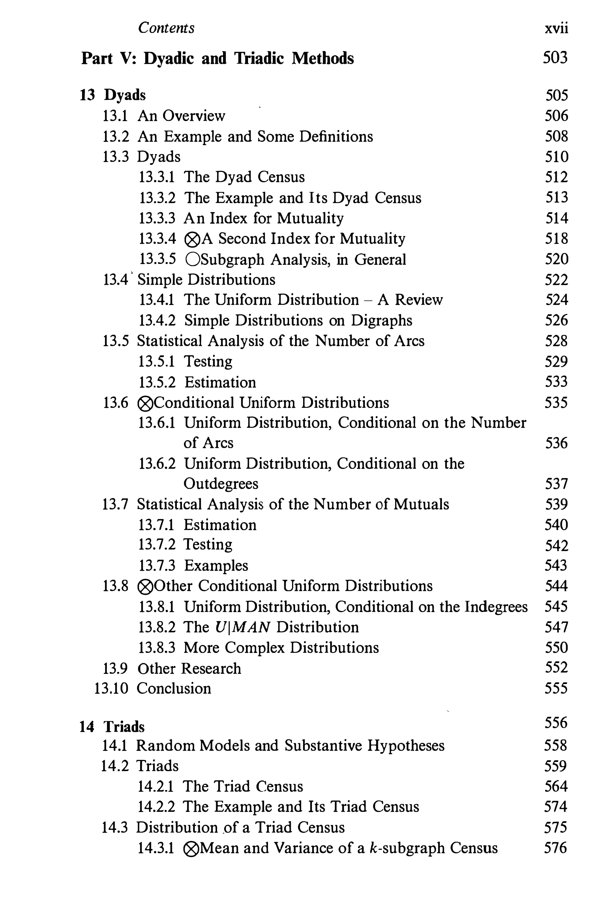
Part V: Dyadic and Triadic Methods 503
13 Dyads 505
13.1 An Overview 506
13.2 An Example and Some Definitions 508
13.3 Dyads 510
13.3.1 The Dyad Census 512
13.3.2 The Example and Its Dyad Census 513
13.3.3 An Index for Mutuality 514
13.3.4 (8)A Second Index for Mutuality 518
13.3.5 OSubgraph Analysis, in General 520
13.4· Simple Distributions 522
13.4.1 The Uniform Distribution - A Review 524
13.4.2 Simple Distributions on Digraphs 526
13.5 Statistical Analysis of the Number of Arcs 528
13.5.1 Testing 529
13.5.2 Estimation 533
13.6 (8)Conditional Uniform Distributions 535
13.6.1 Uniform Distribution, Conditional on the Number
of Arcs 536
13.6.2 Uniform Distribution, Conditional on the
Outdegrees 537
13.7 Statistical Analysis of the Number of Mutuals 539
13.7.1 Estimation 540
13.7.2 Testing 542
13.7.3 Examples 543
13.8 (8)Other Conditional Uniform Distributions 544
13.8.1 Uniform Distribution, Conditional on the Indegrees 545
13.8.2 The UlMAN Distribution 547
13.8.3 More Complex Distributions 550
13.9 Other Research 552
13.10 Conclusion 555
14 Triads 556
14.1 Random Models and Substantive Hypotheses 558
14.2 Triads 559
14.2.1 The Triad Census 564
14.2.2 The Example and Its Triad Census 574
14.3 Distribution of a Triad Census 575
14.3.1 (8)Mean and Variance of a k-subgraph Census 576
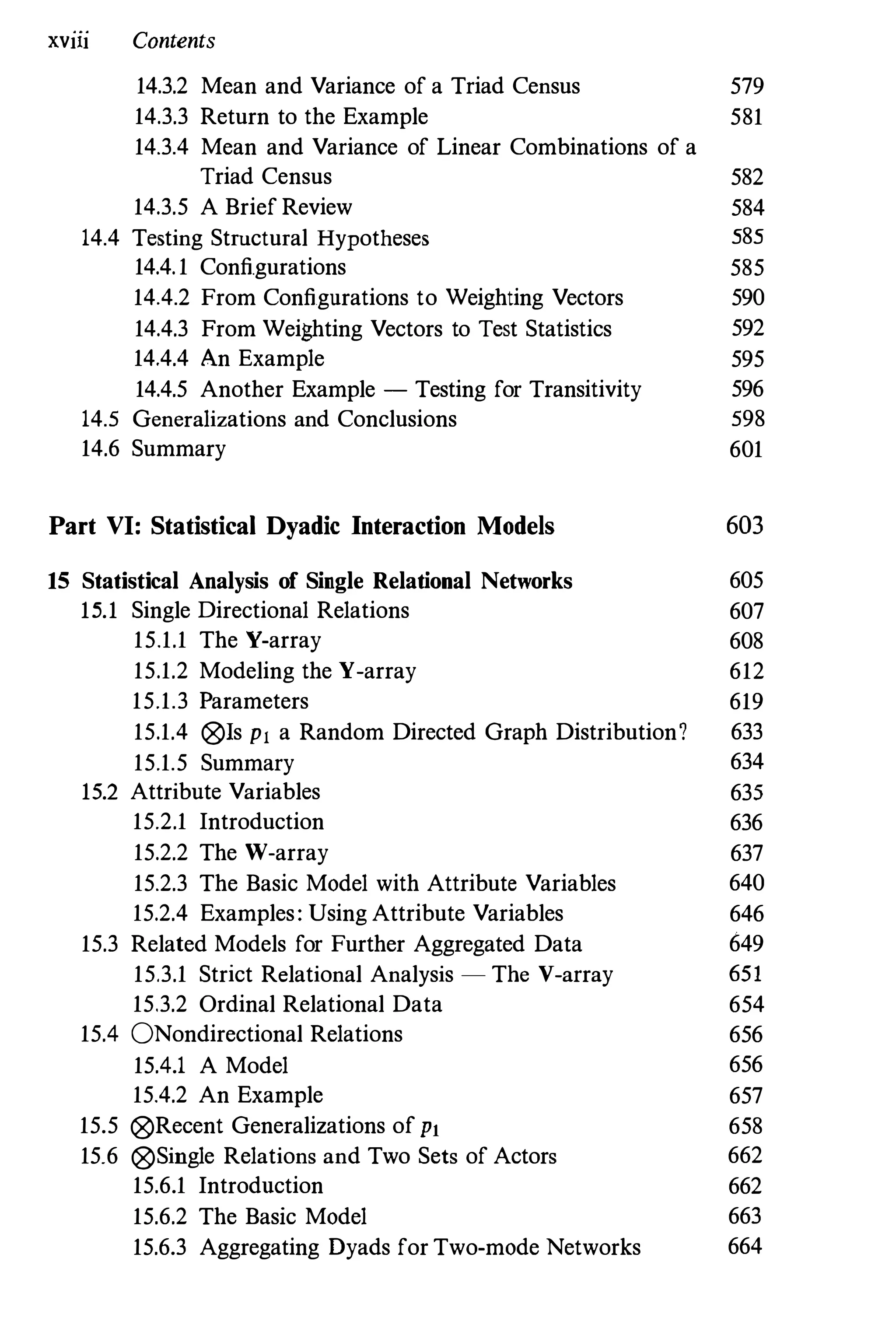
XVlll Contents
14.3.2 Mean and Variance of a Triad Census
14.3.3 Return to the Example
14.3.4 Mean and Variance of Linear Combinations of a
579
581
Triad Census 582
14.3.5 A Brief Review 584
14.4 Testing Structural Hypotheses 585
14.4.1 Configurations 585
14.4.2 From Configurations to Weighting Vectors 590
14.4.3 From Weighting Vectors to Test Statistics 592
14.4.4 An Example 595
14.4.5 Another Example - Testing for Transitivity 596
14.5 Generalizations and Conclusions 598
14.6 Summary 601
Part VI: Statistical Dyadic Interaction Models 603
15 Statistical Analysis of Single Relational Networks 605
15.1 Single Directional Relations 607
15.1.1 The V-array 608
15.1.2 Modeling the Y-array 612
15.1.3 Parameters 619
15.1.4 @ls PI a Random Directed Graph Distribution? 633
15.1.5 Summary 634
15.2 Attribute Variables 635
15.2.1 Introduction 636
15.2.2 The W-array 637
15.2.3 The Basic Model with Attribute Variables 640
15.2.4 Examples: Using Attribute Variables 646
15.3 Related Models for Further Aggregated Data 649
15.3.1 Strict Relational Analysis - The V-array 651
15.3.2 Ordinal Relational Data 654
15.4 ONondirectional Relations 656
15.4.1 A Model 656
15.4.2 An Example 657
15.5 @Recent Generalizations of PI 658
15.6 @Single Relations and Two Sets of Actors 662
15.6.1 Introdnction 662
15.6.2 The Basic Model 663
15.6.3 Aggregating Dyads for Two-mode Networks 664
Contents xix
15.7 Computing for Log-linear Models 665
15.7.1 Computing Packages 666
15.7.2 From Printouts to Parameters 671
15.8 Summary 673
16 Stocbastic B1ockmodels and Goodness-of-Fit Indices 675
16.1 Evaluating B1ockmodels 678
16.1.1 Goodness-of-Fit Statistics for Blockmodels 679
16.1.2 Structurally Based Blockmodels and Permutation
Tests 688
16.1.3 An Example 689
16.2 Stochastic B1ockmodels 692
16.2.1 Definition of a Stochastic Blockmodel 694
16.2.2 Definition of Stochastic Equivalence 696
16.2.3 Application to Special Probability Functions 697
16.2.4 Goodness-of-Fit Indices for Stochastic B1ockmodels 703
16.2.5 OStochastic a posteriori Blockmodels 706
16.2.6 Measures of Stochastic Equivalence 708
16.2.7 Stochastic B1ockmodel Representations 709
16.2.8 The Example Continued 712
16.3 Summary: Generalizations and Extensions 719
16.3.1 Statistical Analysis ofMultiple Relational Networks 719
16.3.2 Statistical Analysis of Longitudinal Relations 721
Part VII: Epilogue 725
17 Future Directions 727
17.1 Statistical Models 727
17.2 Generalizing to New Kinds of Data 729
17.2.1 Multiple Relations 730
17.2.2 Dynamic and Longitudinal Network Models 730
17.2.3 Ego-centered Networks 731
17.3 Data Collection 731
17.4 Sampling 732
17.5 General Propositions about Structure 732
17.6 Computer Technology 733
17.7 Networks and Standard Social and Behavioral Science 733
xx Contents
Appendix A Computer Programs
Appendix B Data
References
Name Index
Subject Index
List ofNotation
735
738
756
802
811
819
List of Tables
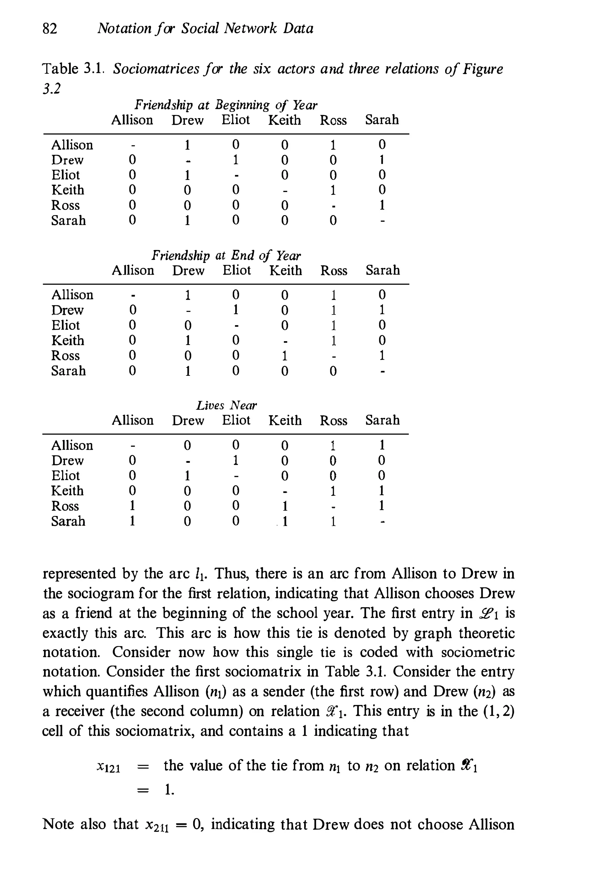
3.1 Sociomatrices for the six actors and three relations of
Figure 3.2 82
3.2 The sociomatrix for the relation "is a stndent of" defined
for heterogeneous pairs from JV and .4t 88
4.1 Nodal degree and density for friendships among Krack-
hardt's high-tech managers 130
4.2 Example of a sociomatrix: "lives near" relation for six
children 151
4.3 Example of an incidence matrix: "lives near" relation for
six children 152
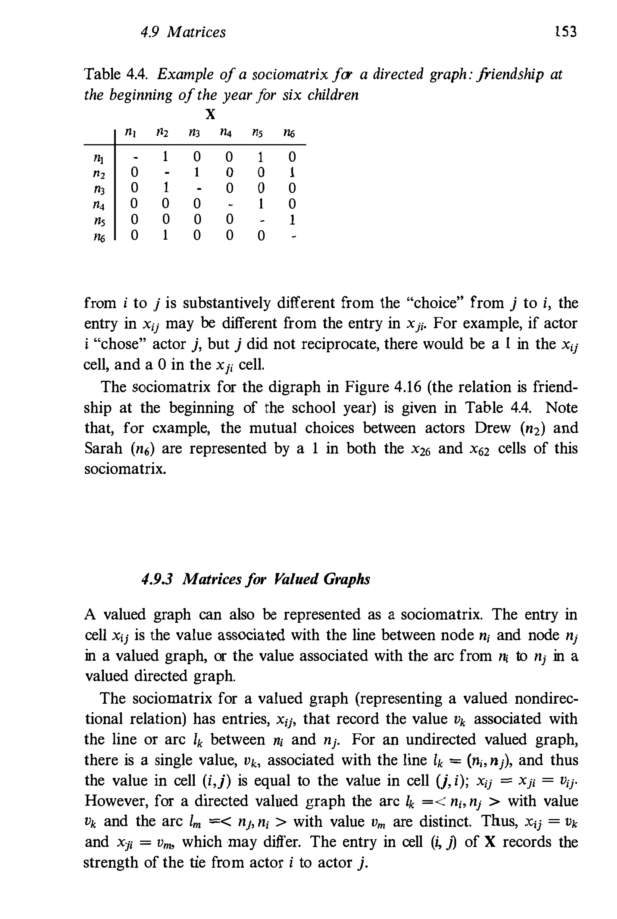
4.4 Example of a sociomatrix for a directed graph: friendship
at the beginning of the year for six children 153
4.5 Example of matrix permutation 156
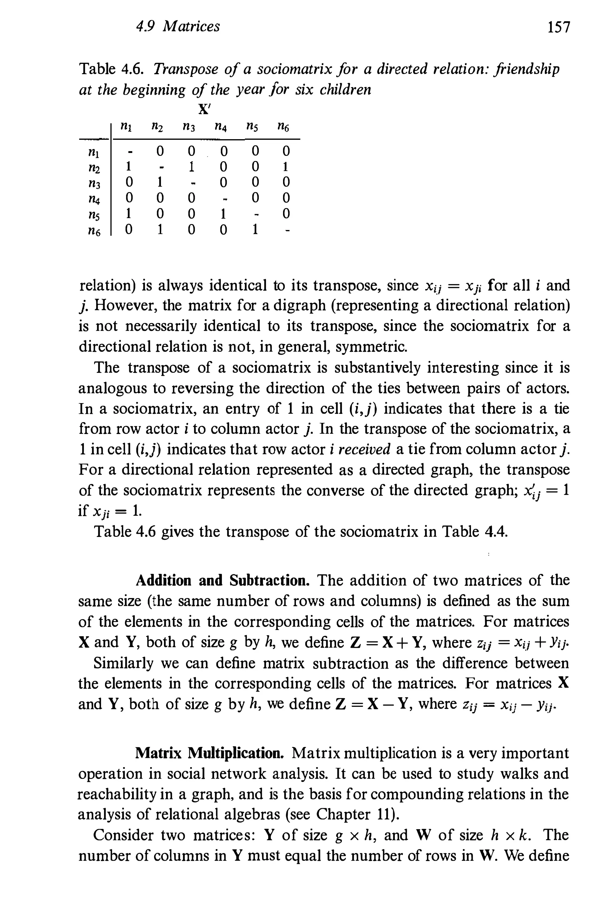
4.6 Transpose of a sociomatrix for a directed relation:
friendship at the beginning of the year for six children 157
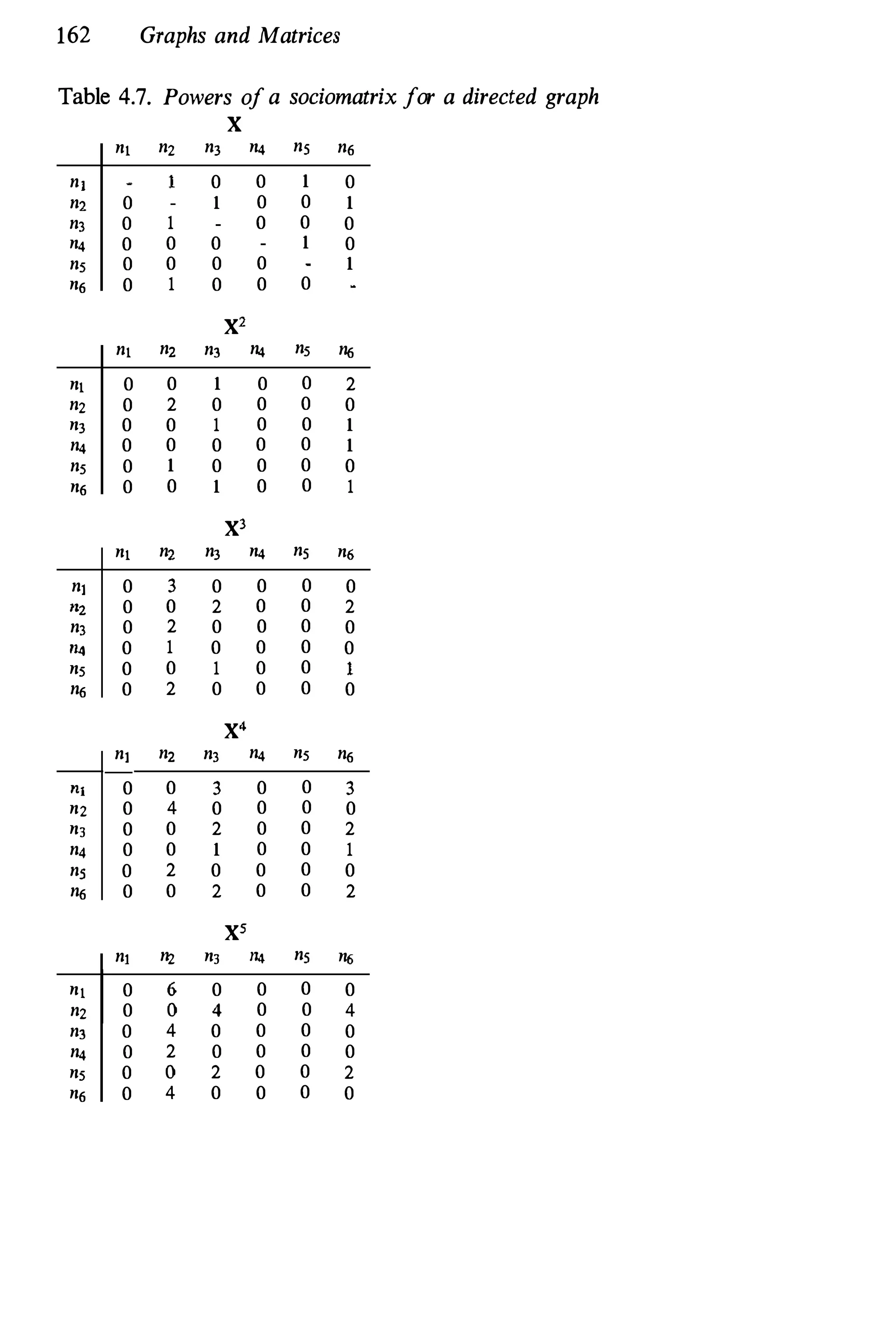
4.7 Powers of a sociomatrix for a directed graph 162
5.1 Centrality indices for Padgett's Florentine families 183
5.2 Centrality for the countries trade network 211
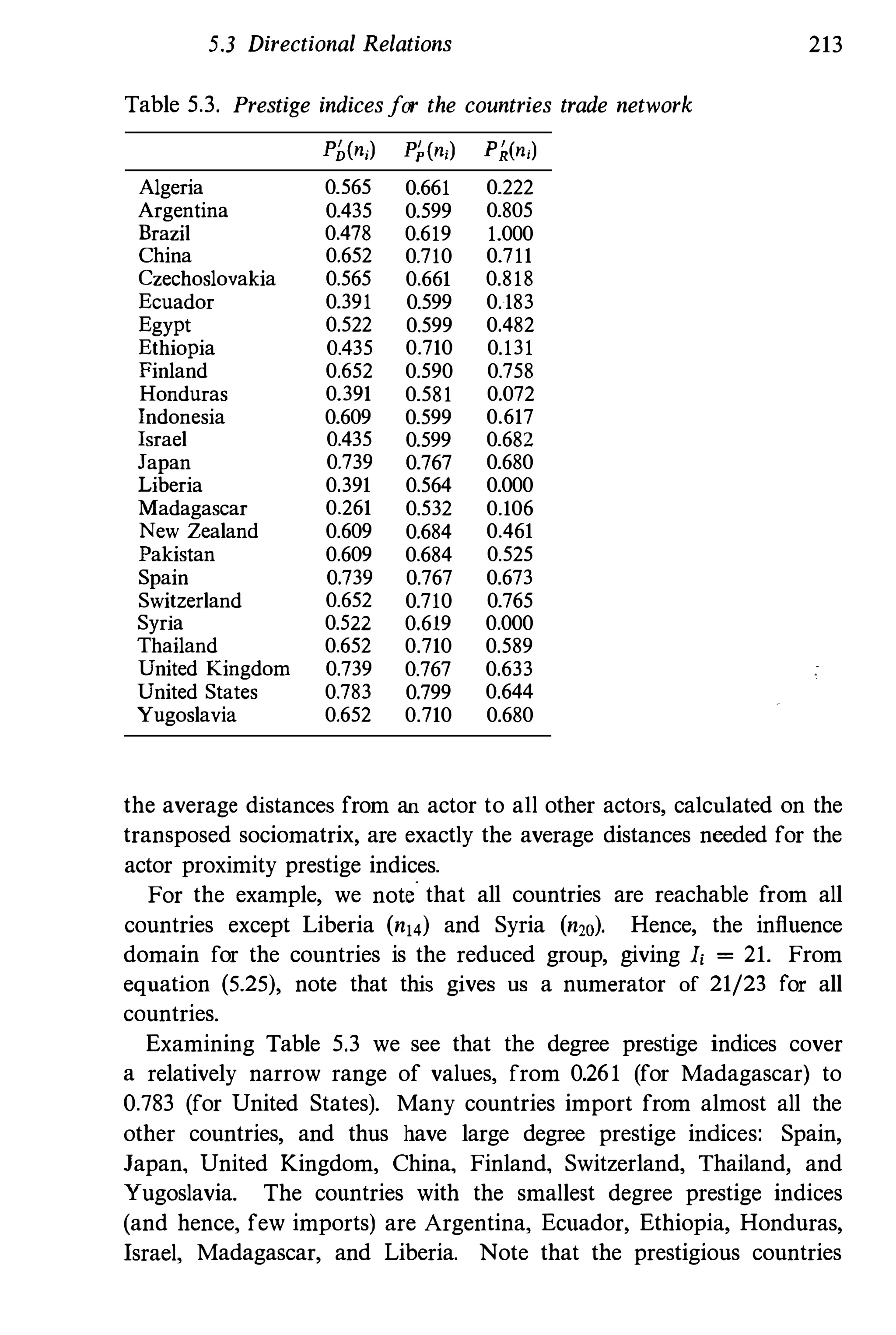
5.3 Prestige indices for the countries trade network 213
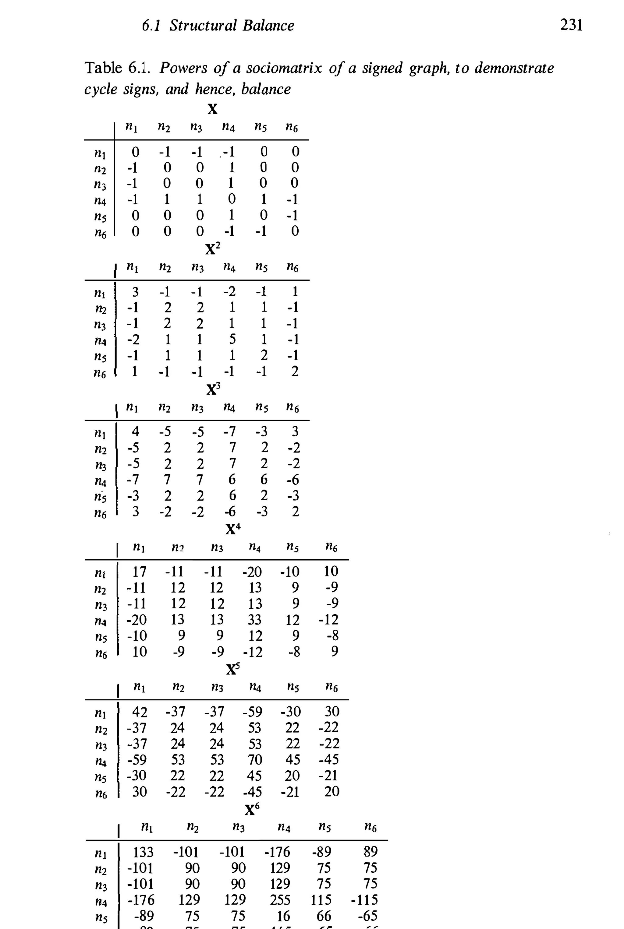
6.1 Powers ofa sociomatrix of a signed graph, to demonstrate
cycle signs, and hence, balance 231
8.1 Cliques in the actor co-membership relation for Galaskie-
wicz's CEOs and clubs network 321
8.2 Cliques in the event overlap relation for Galaskiewicz's
CEOs and clubs network 321
8.3 Correspondence analysis scores for CEOs and clubs 341
10.1 Mean age and tenure of actors in positions for Krack-
hardt's high-tech managers (standard deviations in
parentheses) 410
xxi
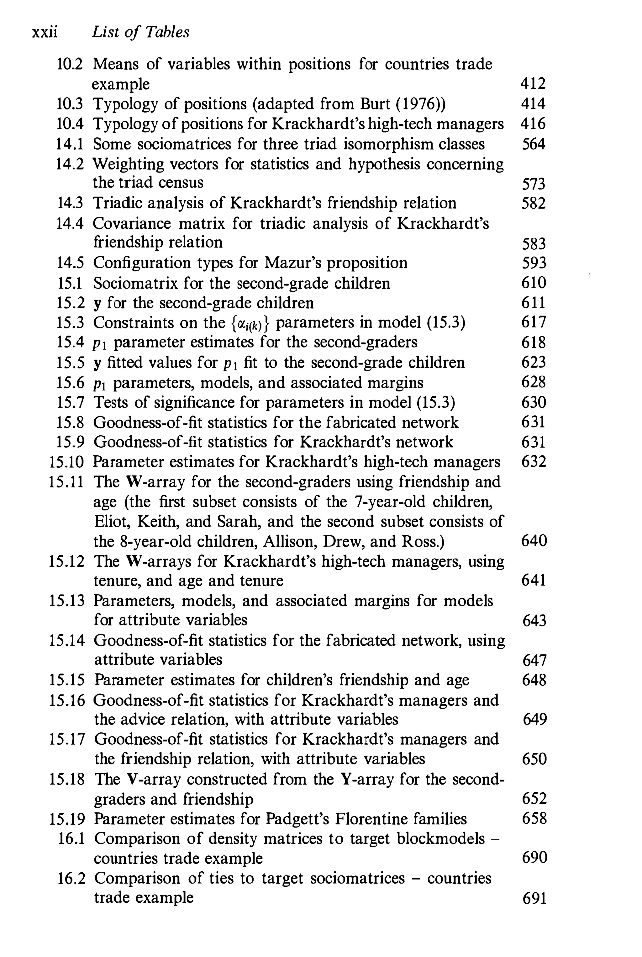
xxn List of Tables
10.2 Means of variables within positions for countries trade
example 412
10.3 Typology of positions (adapted from Burt (1976)) 414
10.4 Typology ofpositions for Krackhardt's high-tech managers 416
14.1 Some sociomatrices for three triad isomorphism classes 564
14.2 Weighting vectors for statistics and hypothesis concerning
the triad census 573
14.3 Triadic analysis of Krackhardt's friendship relation 582
14.4 Covariance matrix for triadic analysis of Krackhardt's
friendship relation 583
14.5 Configuration types for Mazur's proposition 593
15.1 Sociomatrix for the second-grade children 610
15.2 y for the second-grade children 611
15.3 Constraints on the {�i(k)} parameters in model (15.3) 617
15.4 PI parameter estimates for the second-graders 618
15.5 y fitted values for PI fit to the second-grade children 623
15.6 PI parameters, models, and associated margins 628
15.7 Tests of significance for parameters in model (15.3) 630
15.8 Goodness-of-fit statistics for the fabricated network 631
15.9 Goodness-of-fit statistics for Krackhardt's network 631
15.10 Parameter estimates for Krackhardt's high-tech managers 632
15.11 The W-array for the second-graders using friendship and
age (the first subset consists of the 7-year-old children,
Eliot, Keith, and Sarah, and the second subset consists of
the 8-year-old children, Allison, Drew, and Ross.) 640
15.12 The W-arrays for Krackhardt's high-tech managers, using
tenure, and age and tenure 641
15.13 Parameters, models, and associated margins for models
for attribute variables 643
15.14 Goodness-of-fit statistics for the fabricated network, using
attribute variables 647
15.15 Parameter estimates for children's friendship and age 648
15.16 Goodness-of-fit statistics for Krackhardt's managers and
the advice relation, with attribute variables 649
15.17 Goodness-of-fit statistics for Krackhardt's managers and
the friendship relation, with attribute variables 650
15.18 The V-array constructed from the Y-array for the second-
graders and friendship 652
15.19 Parameter estimates for Padgett's Florentine families 658
16.1 Comparison of density matrices to target blockmodels -
countries trade example 690
16.2 Comparison of ties to target sociomatrices - countries
trade example 691
List of Tables xxiii
16.3 Fit statistics for PI and special cases 712
16.4 Fit statistics for PI stochastic blockmodels 715
16.5 Predicted density matrix 717
B.l Advice relation between managers of Krackhardt's high-
tech company 740
B.2 Friendship relation between managers of Krackhardt's
high-tech company 741
B.3 "Reports to" relation between managers of Krackhardt's
high-tech company 742
B.4 Attributes for Krackhardt's high-tech managers 743
B.5 Business relation between Florentine fantilies 743
B.6 Marital relation between Florentine families 744
B.7 Attributes for Padgett's Florentine fantilies 744
B.8 Acquaintanceship at time I between Freeman's EIES
researchers 745
B.9 Acquaintanceship at time 2 between Freeman's EIES
researchers 746
B.IO Messages sent between Freeman's EIES researchers 747
B.ll Attributes for Freeman's EIES researchers 748
B.12 Trade of basic manufactured goods between countries 749
B.13 Trade of food and live animals between countries 750
B.14 Trade of crude materials, excluding food 751
B.l5 Trade of ntinerals, fuels, and other petroleum products
between countries 752
B.16 Exchange of diplomats between countries 753
B.17 Attributes for countries trade network 754
B.18 CEOs and clubs affiliation network matrix 755
List of Illustrations
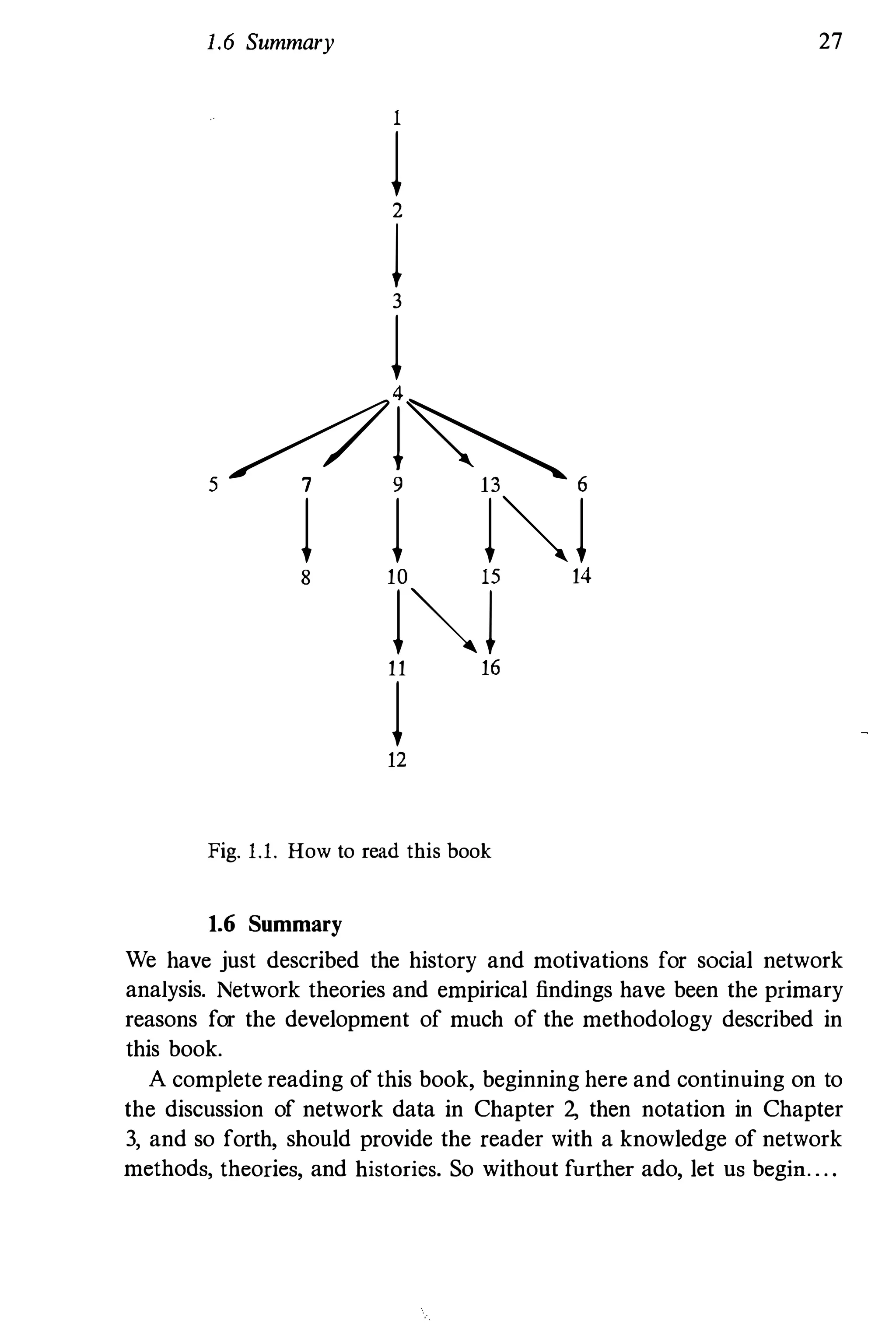
1.1 How to read this book 27
3.1 The six actors and the directed lines between them - a
sociogram 74
3.2 The six actors and the three sets of directed lines - a
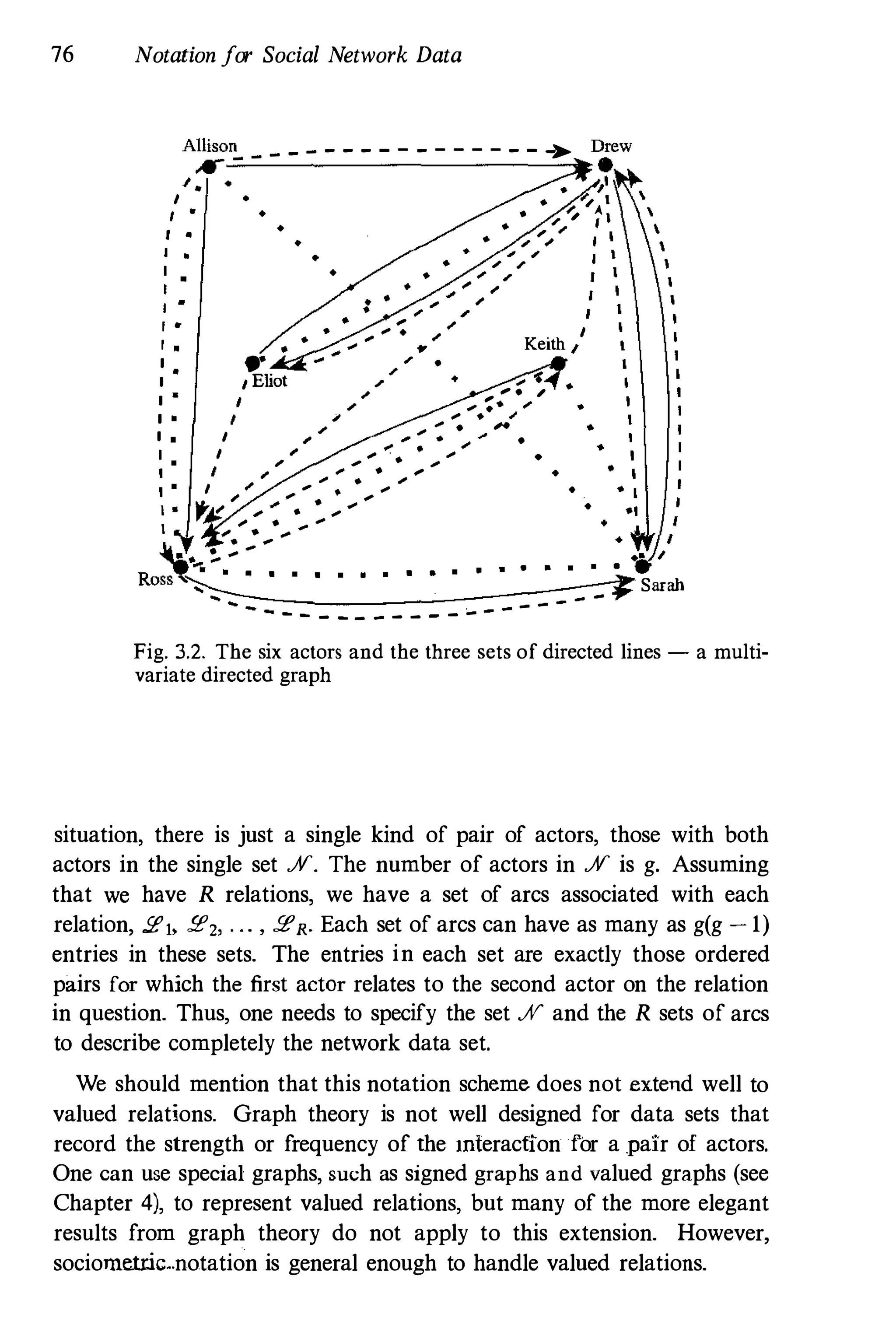
multivariate directed graph 76
4.1 Graph of "lives near" relation for six children 96
4.2 Subgraphs of a graph 98
4.3 Four possible triadic states in a graph 100
4.4 Complete and empty graphs 102
4.5 Graph and nodal degrees for Padgett's Florentine families,
marriage relation 104
4.6 Walks, trails, and paths in a graph 106
4.7 Closed walks and cycles in a graph 108
4.8 A connected graph and a graph with components 109
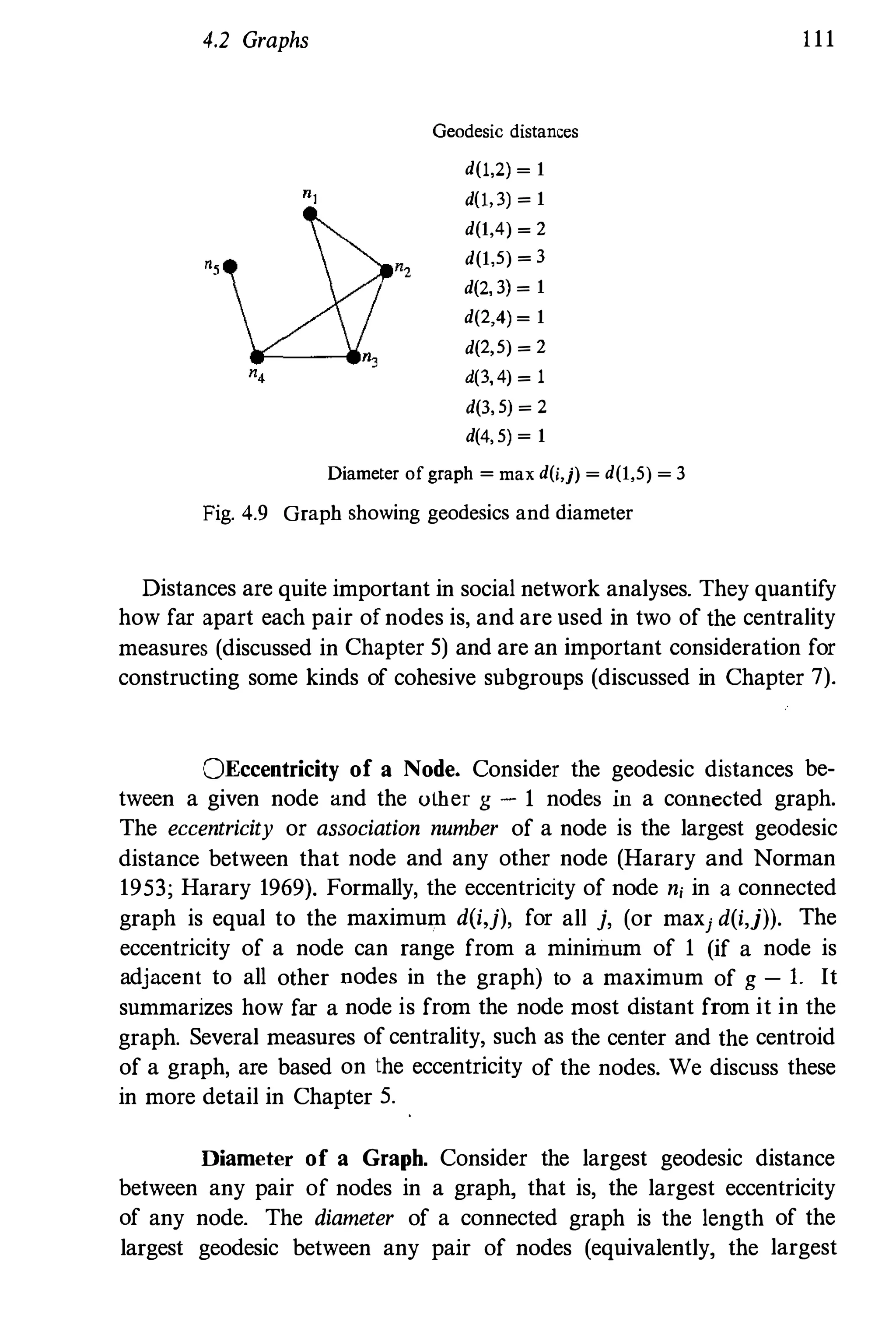
4.9 Graph showing geodesics and diameter 111
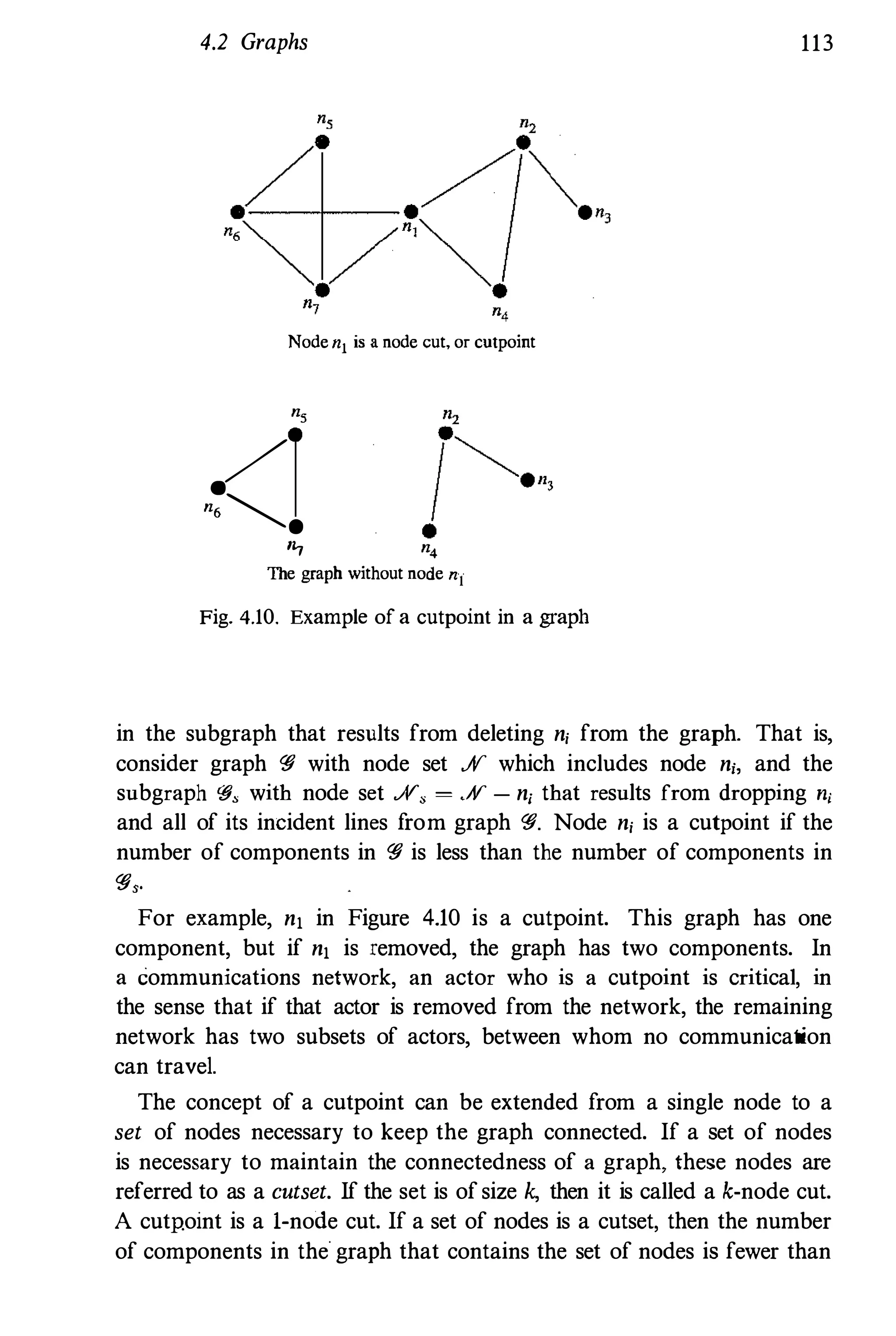
4.10 Example of a cutpoint in a graph 113
4.11 Example of a bridge in a graph 114
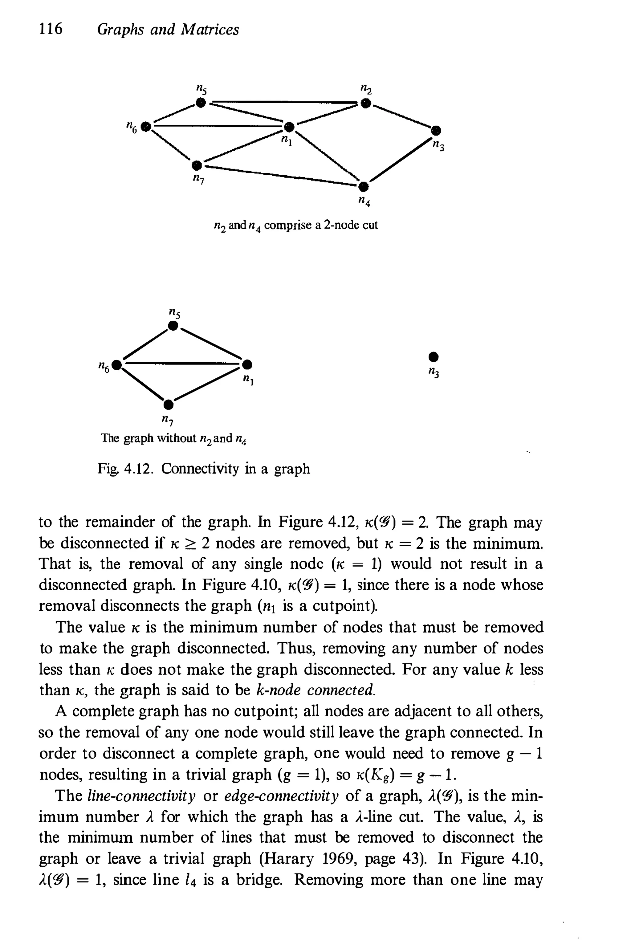
4.12 Connectivity in a graph 116
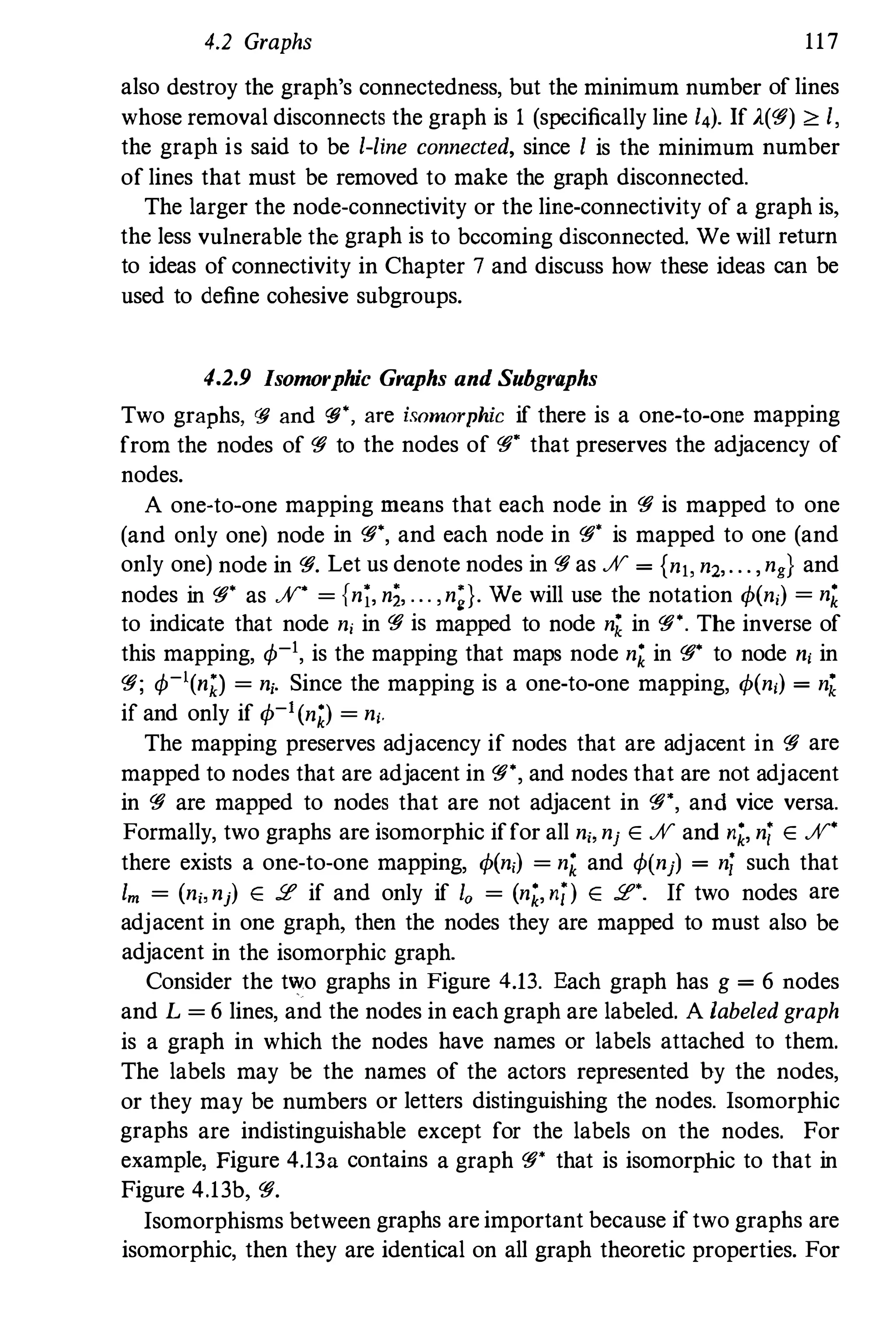
4.13 Isomorphic graphs 118
4.14 Cyclic and acyclic graphs 119
4.15 Bipartite graphs 120
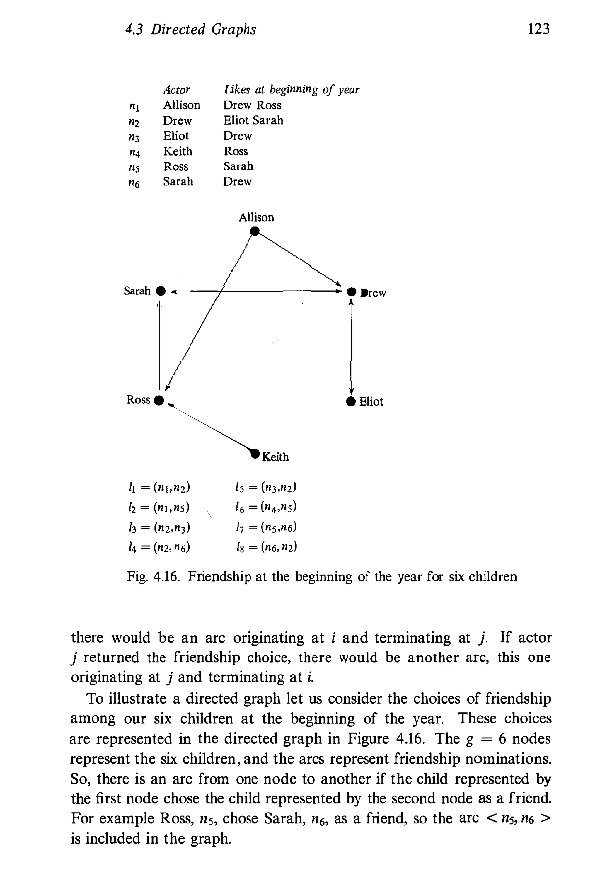
4.16 Friendship at the beginning of the year for six children 123
4.17 Dyads from the graph of friendship among six children at
the beginning of the year 125
4.18 Directed walks, paths, semipaths, and.semicycles 131
4.19 Different kinds of connectivity in a directed graph 133
4.20 Converse and complement of a directed graph 135
4.21 Example of a signed graph 138
4.22 Example of a signed directed graph 139
4.23 Example of a valued directed graph 142
xxiv
List ofIllustrations xxv
4.24 Paths in a valued graph 145
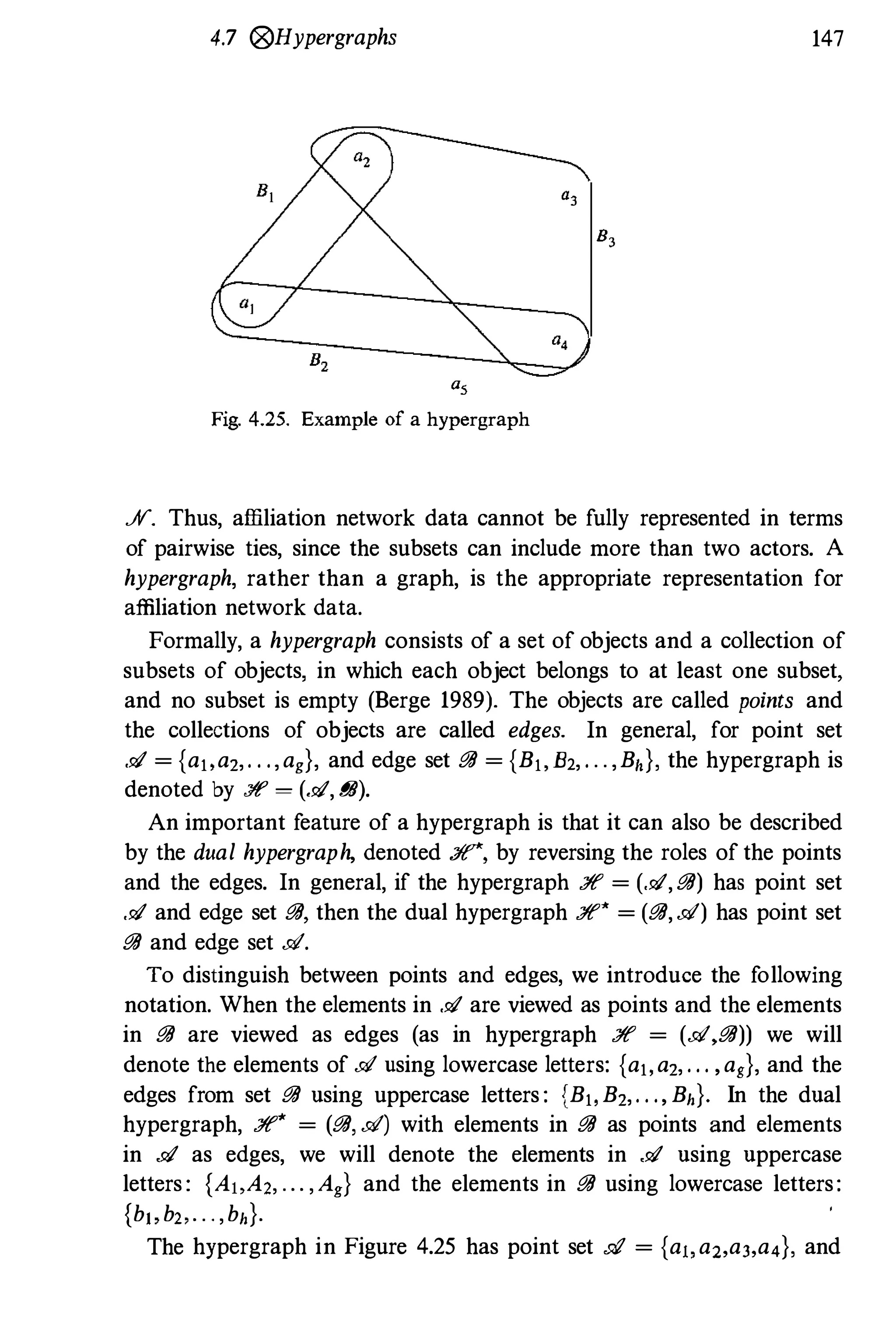
4.25 Example of a hypergraph 147
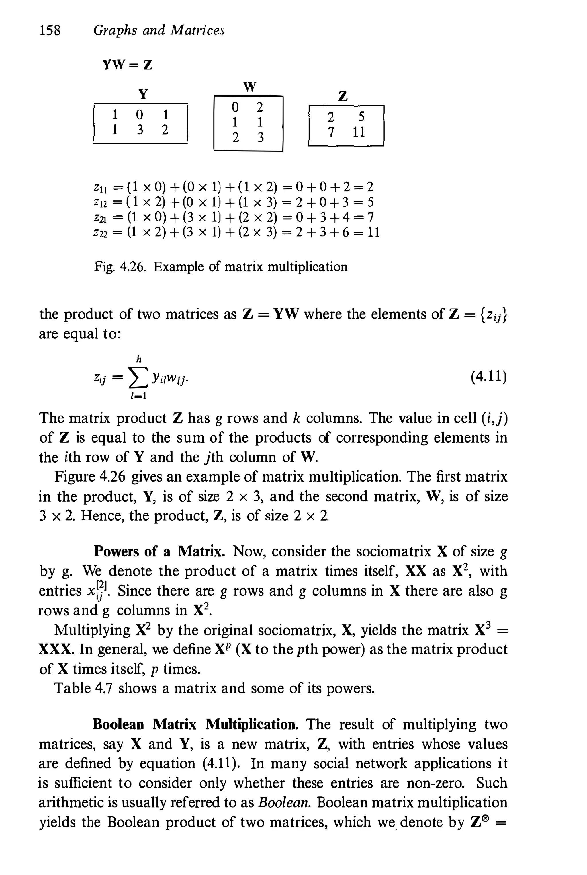
4.26 Example of matrix multiplication 158
5.1 Three illustrative networks for the study of centrality and
prestige 171
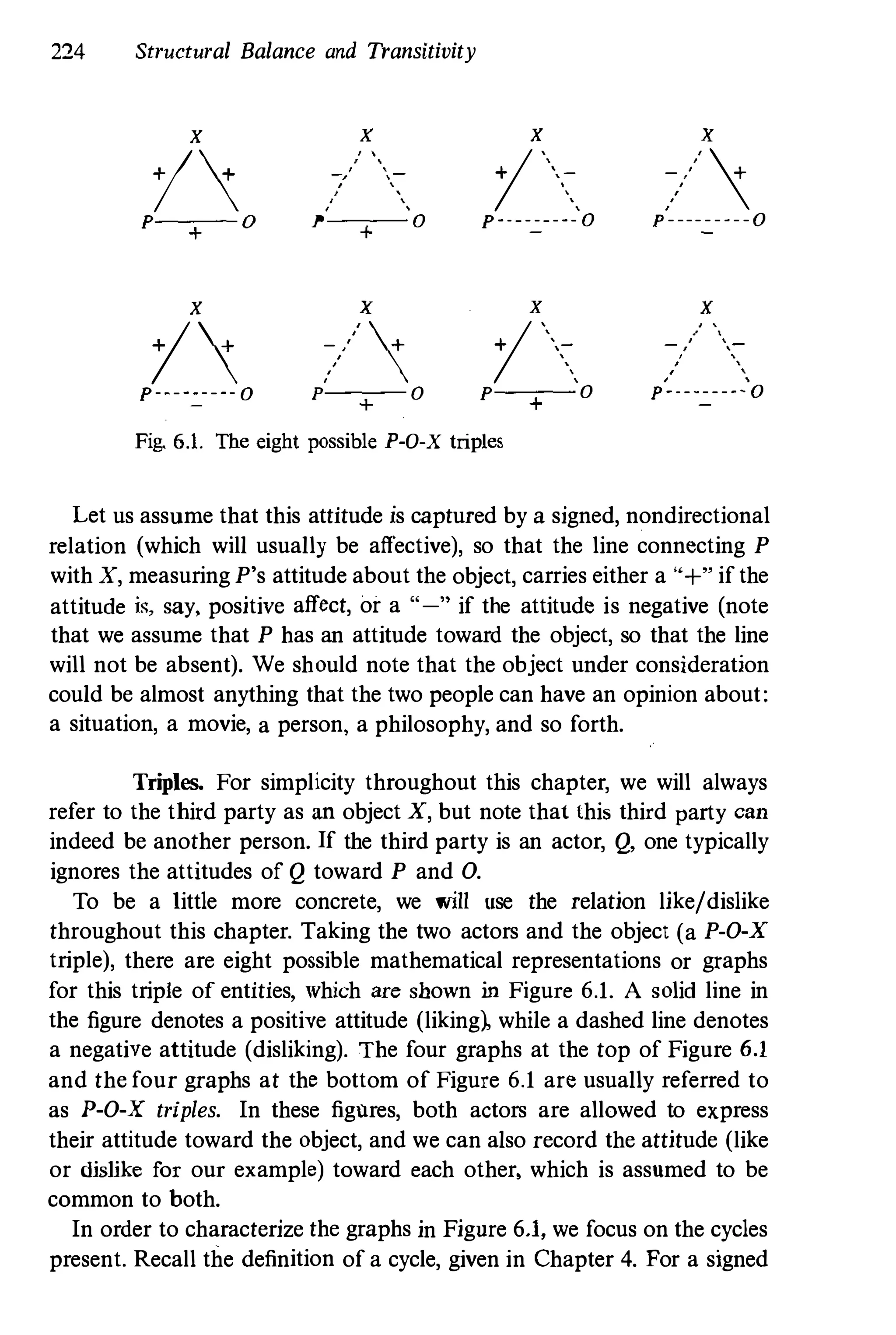
6.1 The eight possible P-O-X triples 224
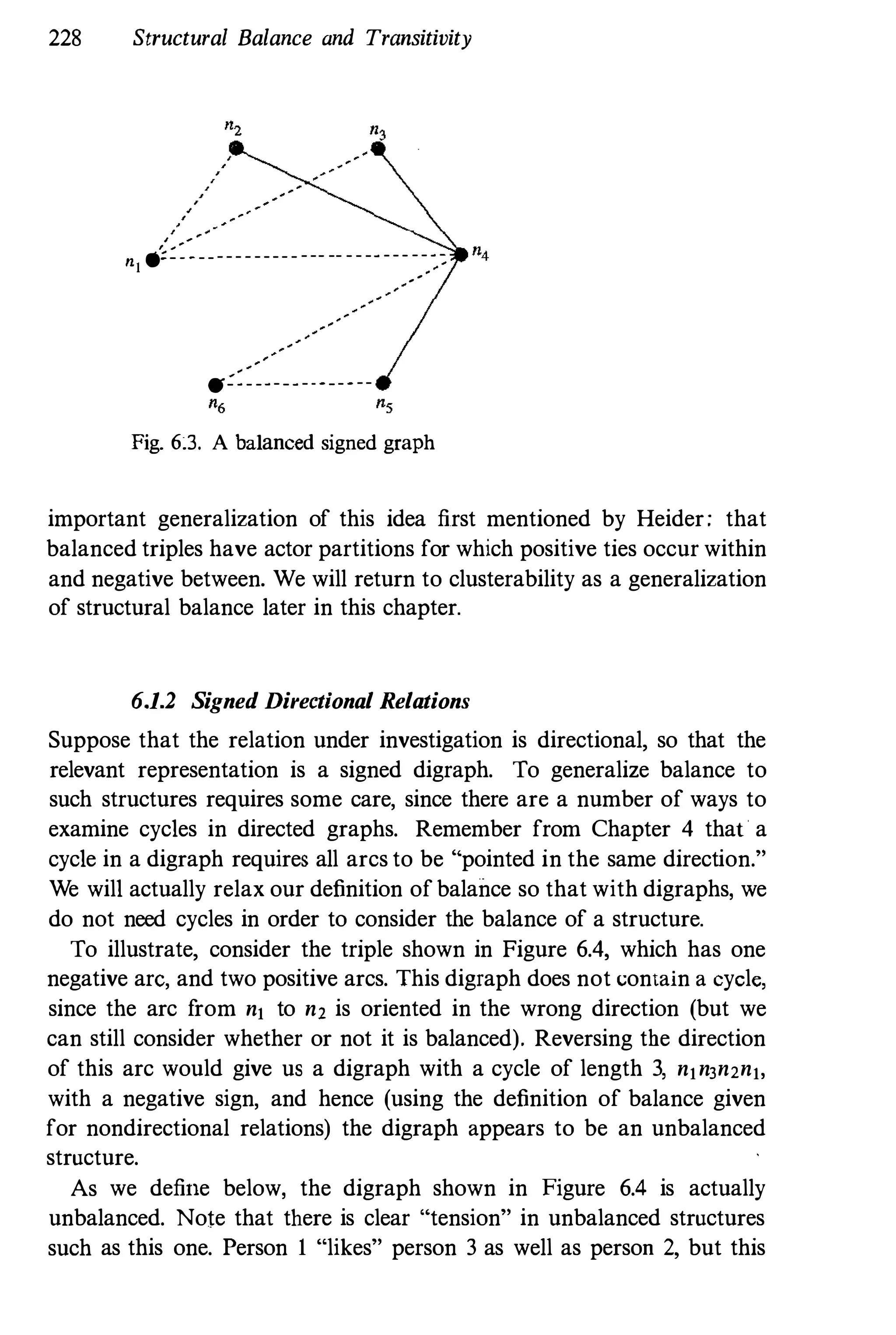
6.2 An unbalanced signed graph 227
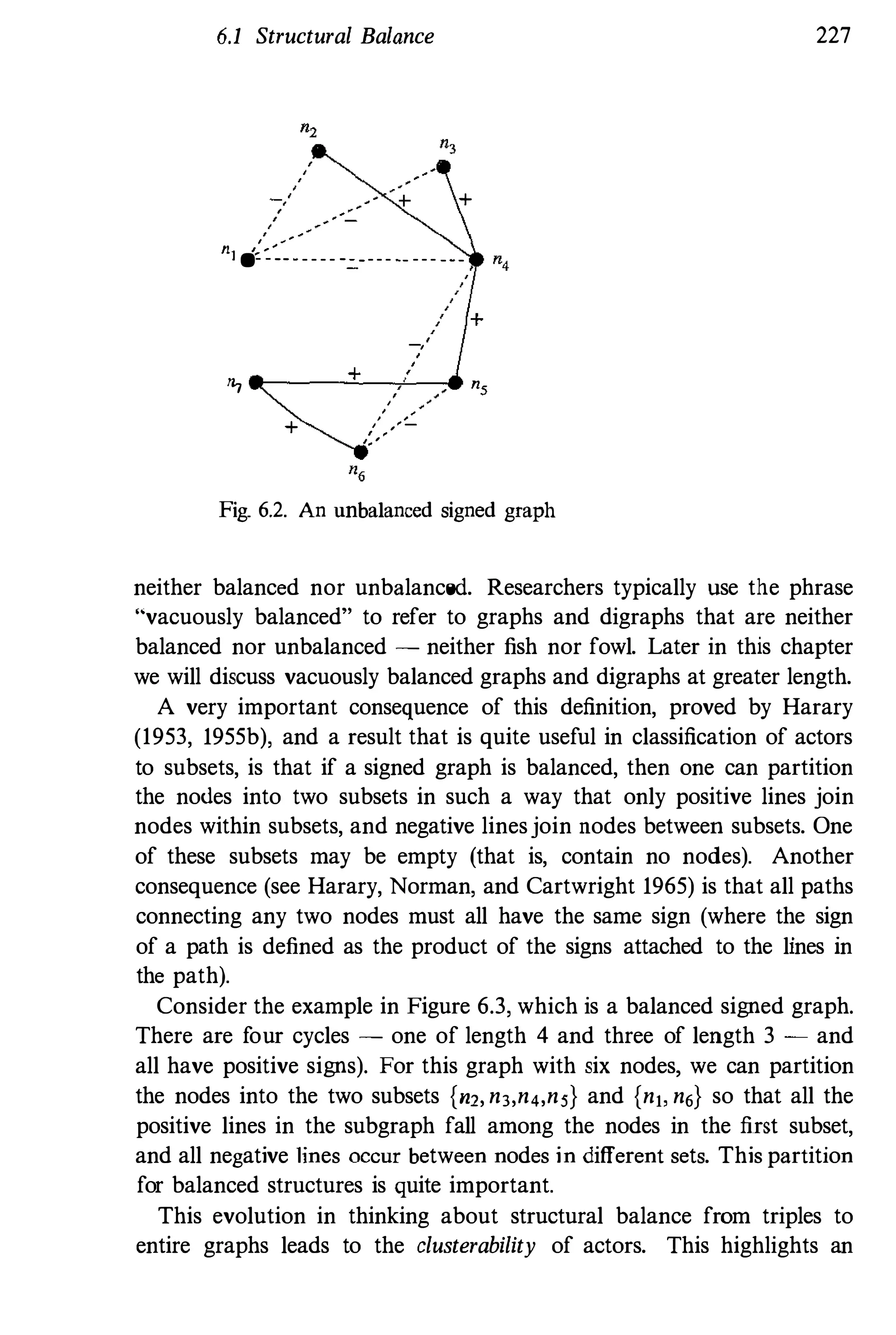
6.3 A balanced signed graph 228
6.4 An unbalanced signed digraph 229
6.5 A clusterable signed graph (with no unique clustering) 236
6.6 The sixteen possible triads for ranked clusterability in a
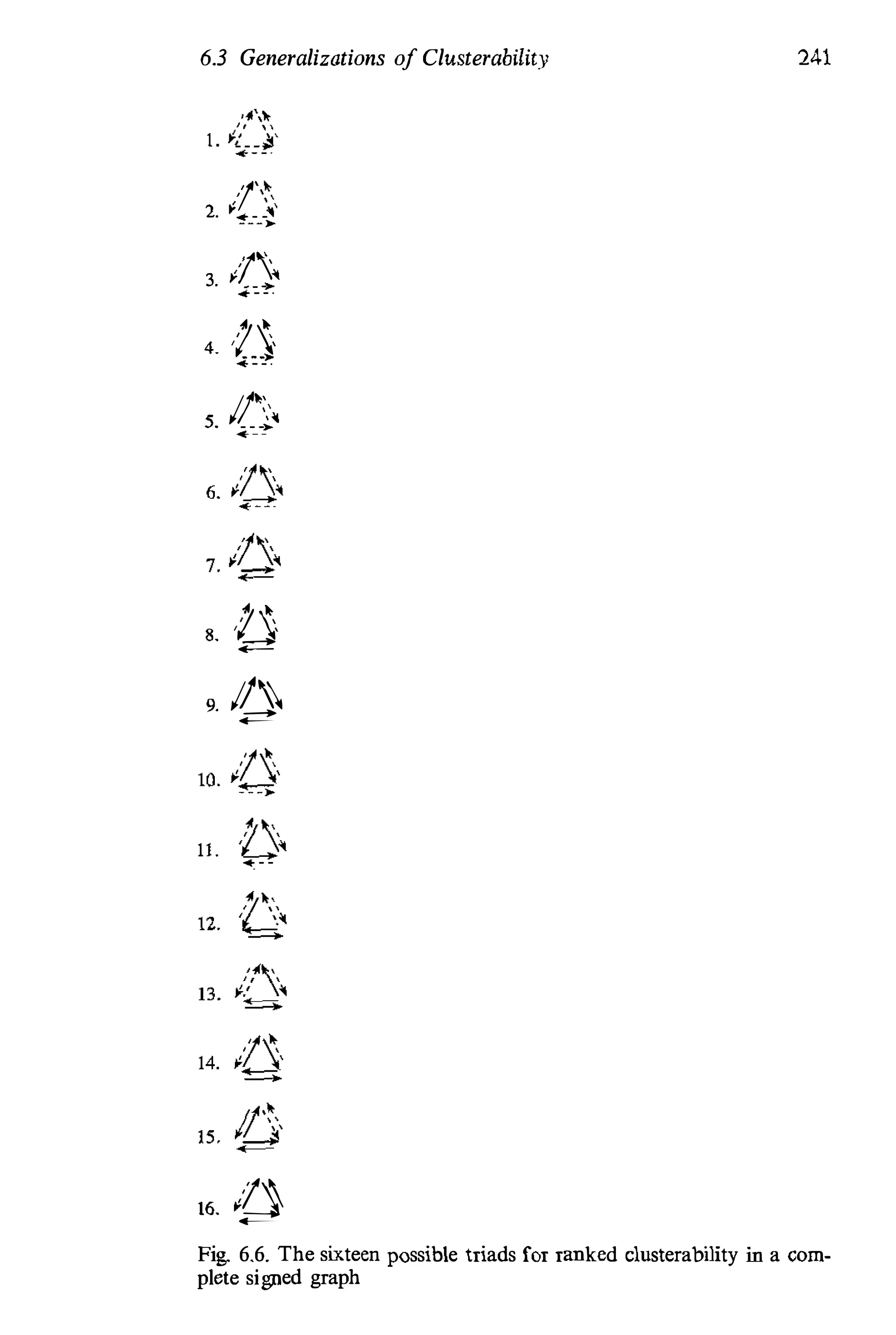
complete signed graph 241
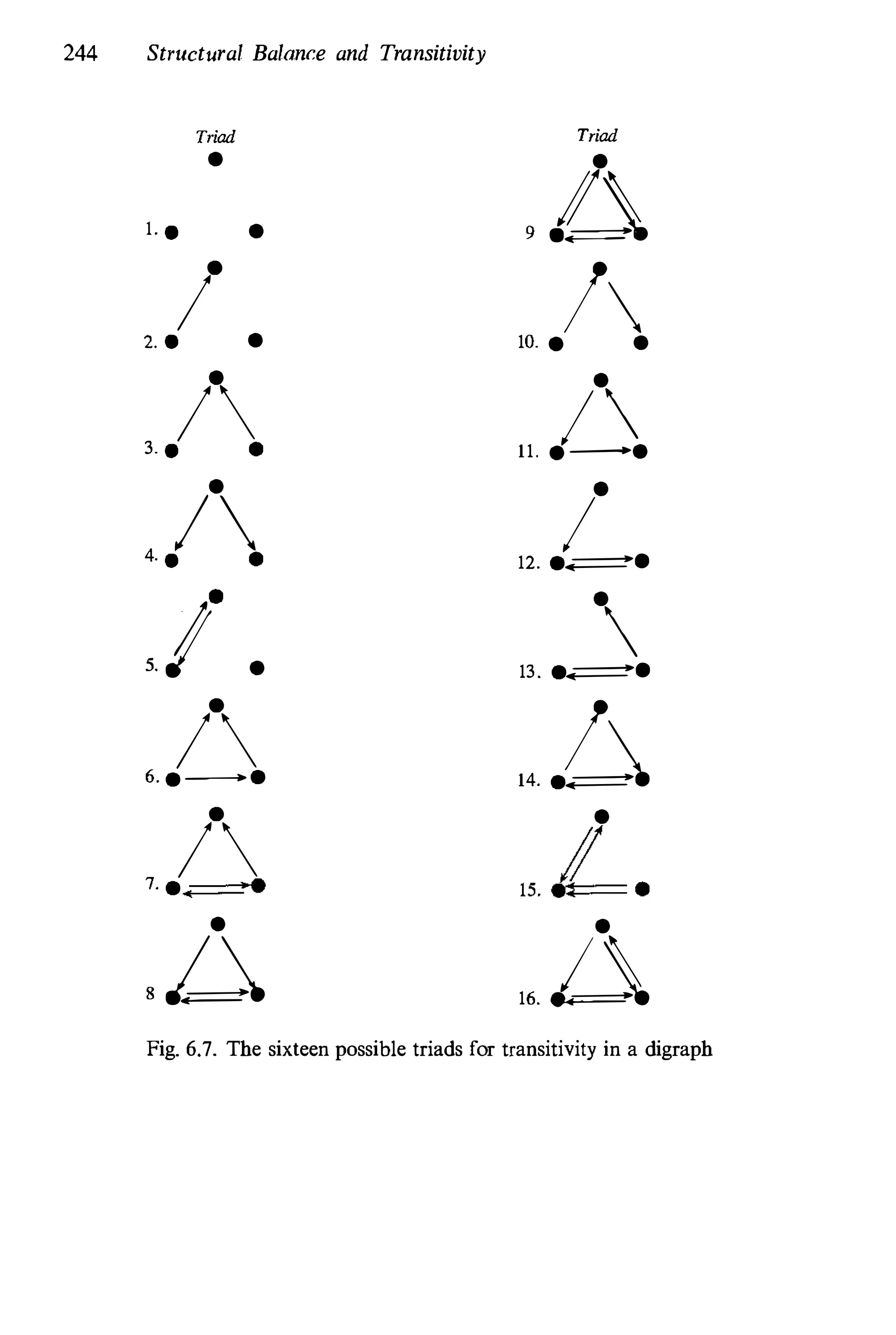
6.7 The sixteen possible triads for transitivity in a digraph 244
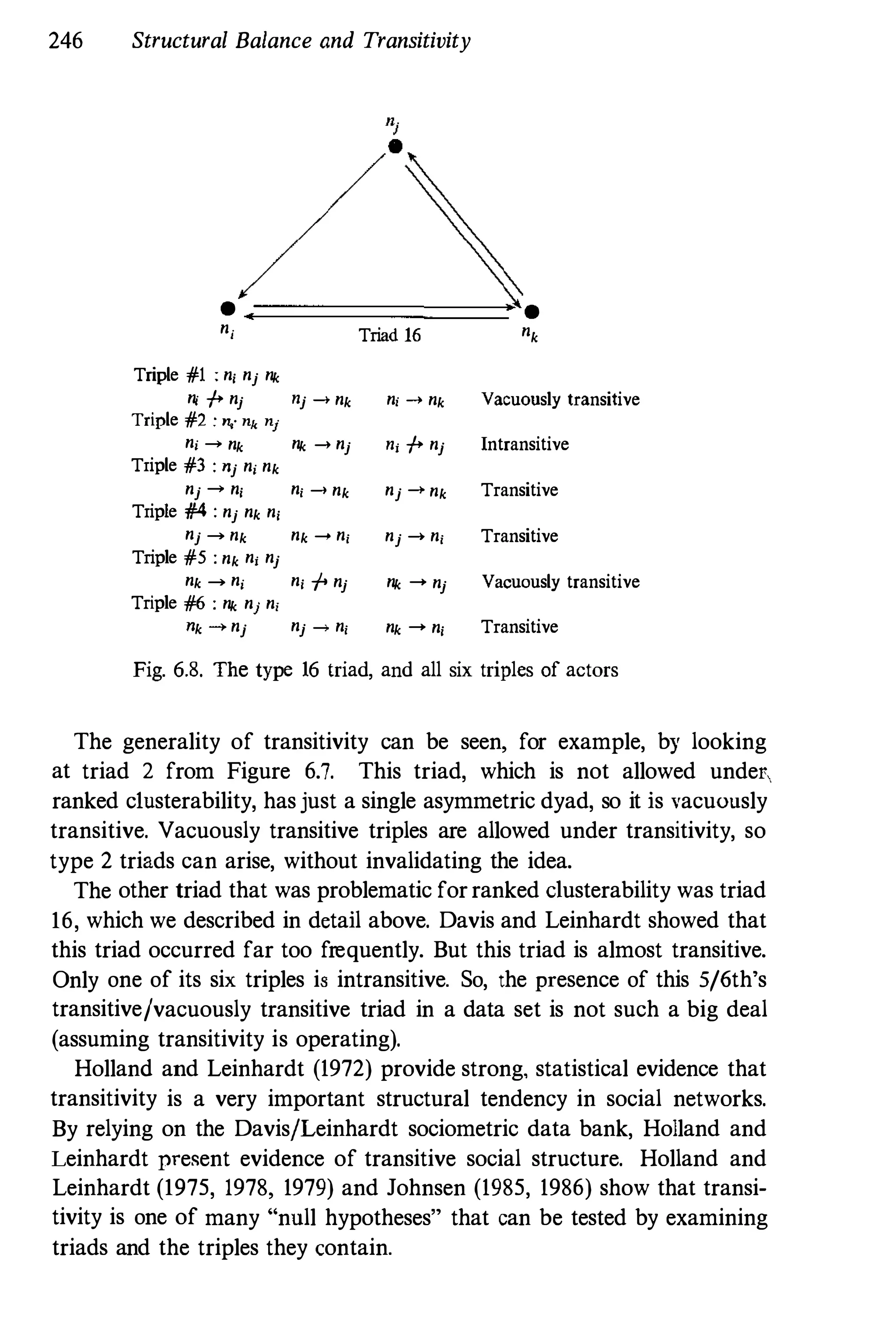
6.8 The type 16 triad, and all six triples of actors 246
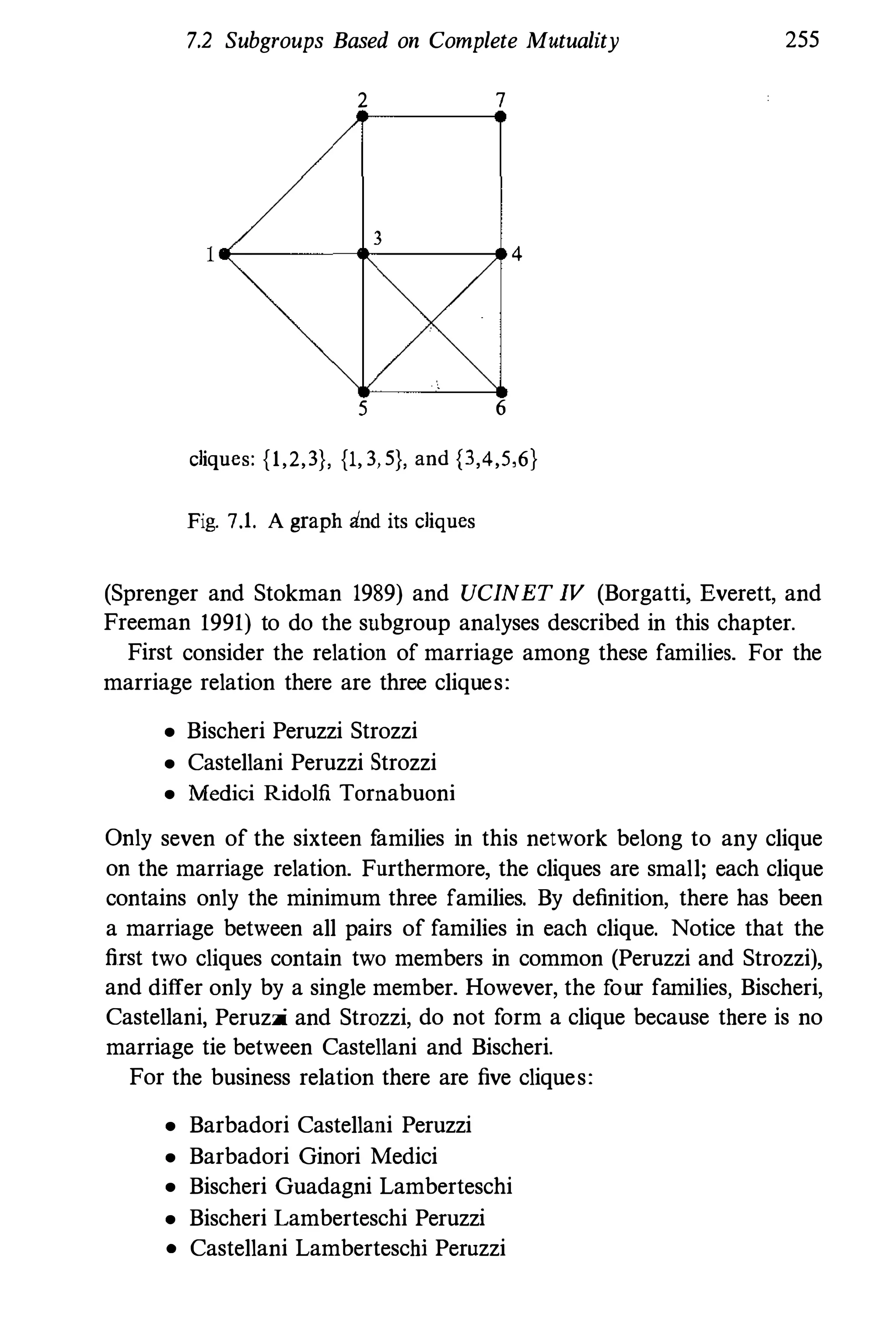
7.1 A graph and its cliques 255
7.2 Graph illustrating n-cliques, n-clans, and n-clubs 259
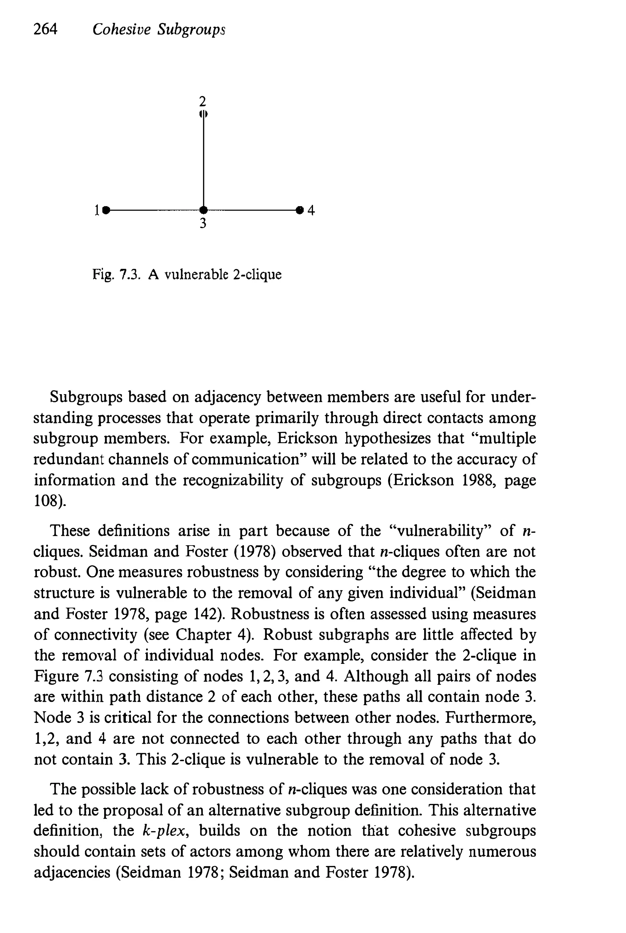
7.3 A vulnerable 2-clique 264
7.4 A valued relation and derived graphs 281
7.5 A hypothetical example showing a permuted sociomatrix 286
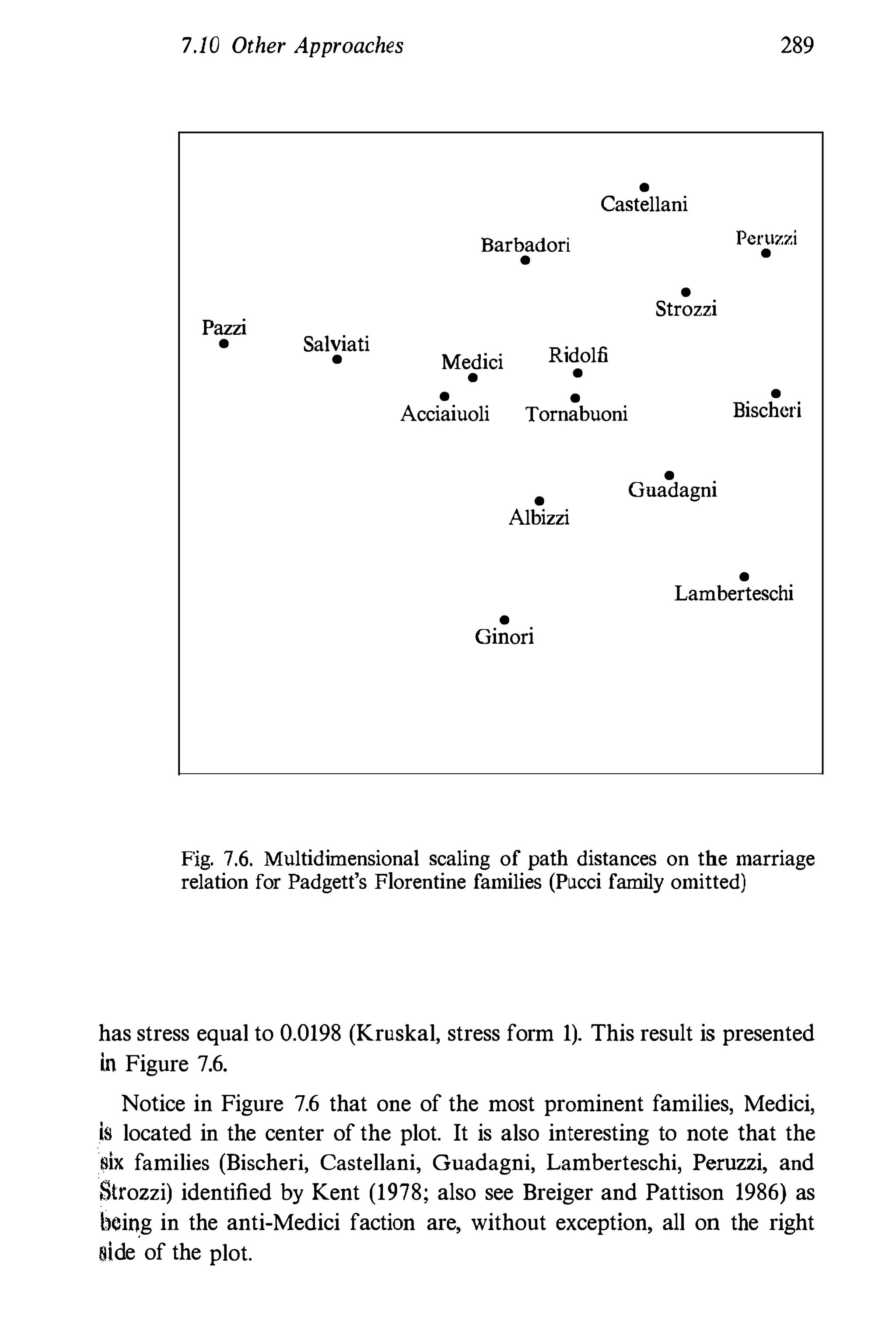
7.6 Multidimensional scaling ofpath distances on the marriage
relation for Padgett's Florentine families (Pucci family
omitted) 289
8.1 Affiliation network matrix for the example of six children
and three birthday parties 299
8.2 Bipartite graph of affiliation network of six children and
three parties 301
8.3 Sociomatrix for the bipartite graph of six children and
three parties 302
8.4 Hypergraph and dual hypergraph for example of six
children and three parties 305
8.5 Actor co-membership matrix for the six children 310
8.6 Event overlap matrix for the three parties 310
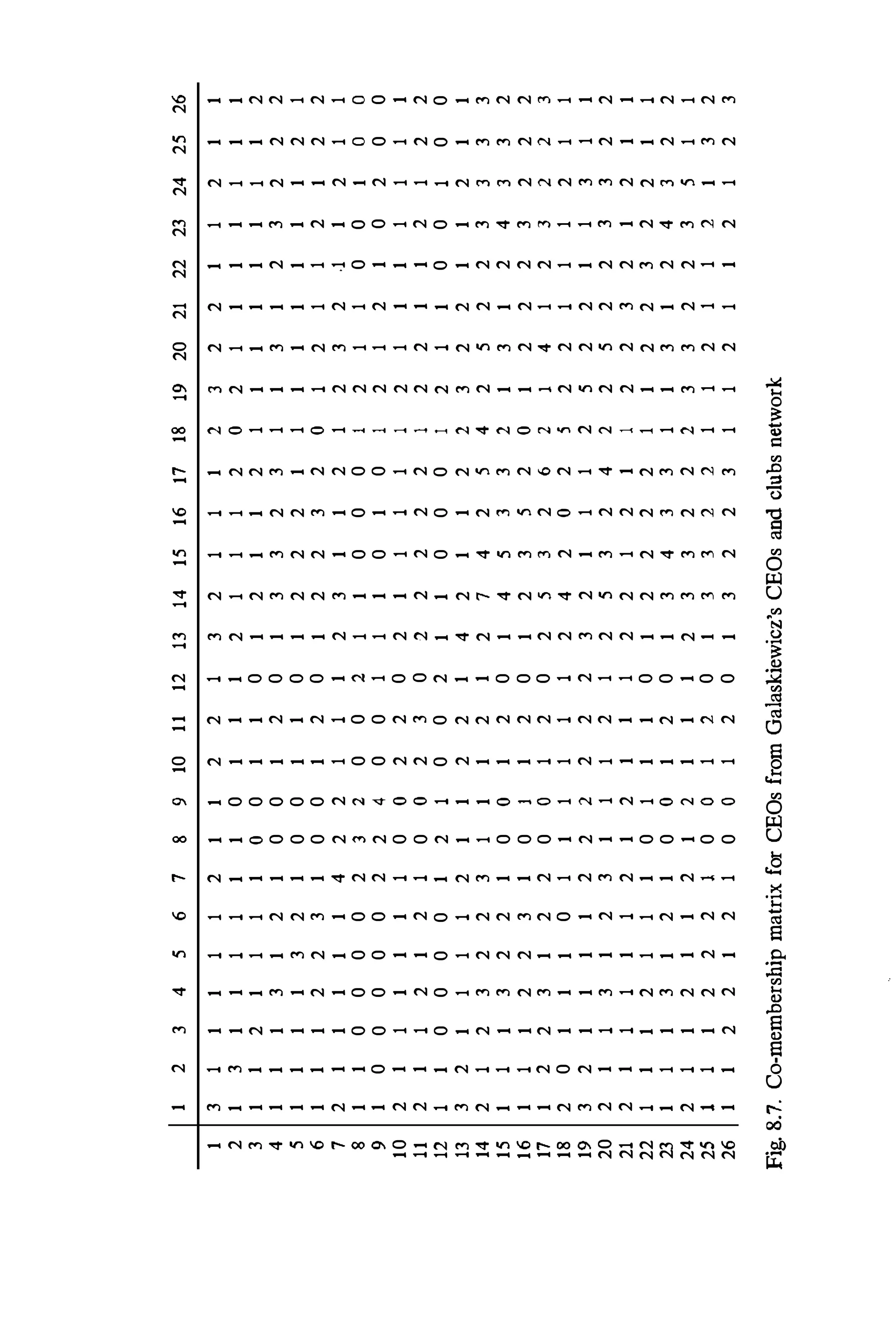
8.7 Co-membership matrix for CEOs from Galaskiewicz's
CEOs and clubs network 311
8.8 Event overlap matrix for clubs from Galaskiewicz's CEOs
and clubs data 313
8.9 Relationships among birthday parties as subsets of
children 329
8.10 Relationships among children as subsets of birthday
parties 330
8.11 Galois lattice of children and birthday parties 333
xxvi List ofIllustrations
8.12 Plot of correspondence analysis scores for CEOs and
clubs example � CEOs in principal coordinates clubs in
standard coordinates 340
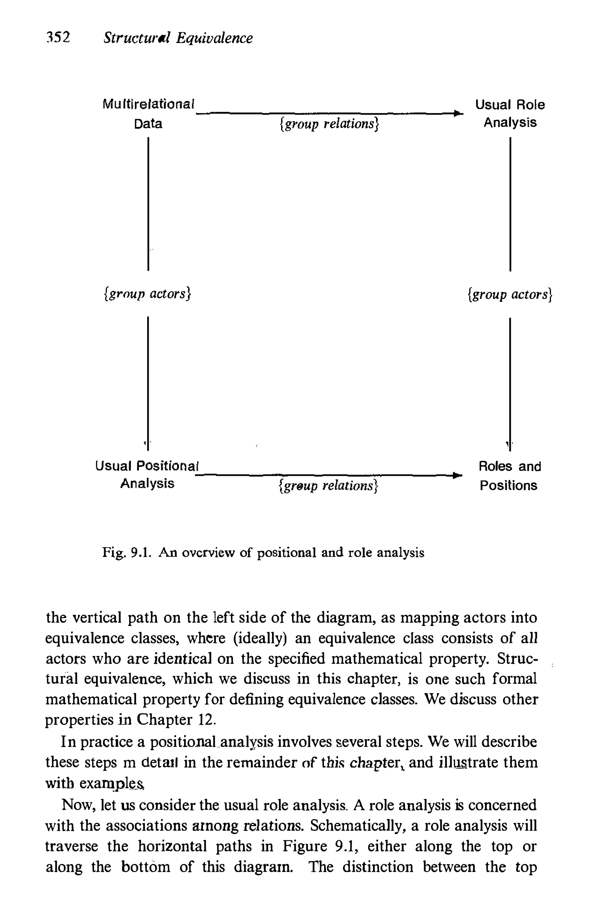
9.1 An overview of positional and role analysis 352
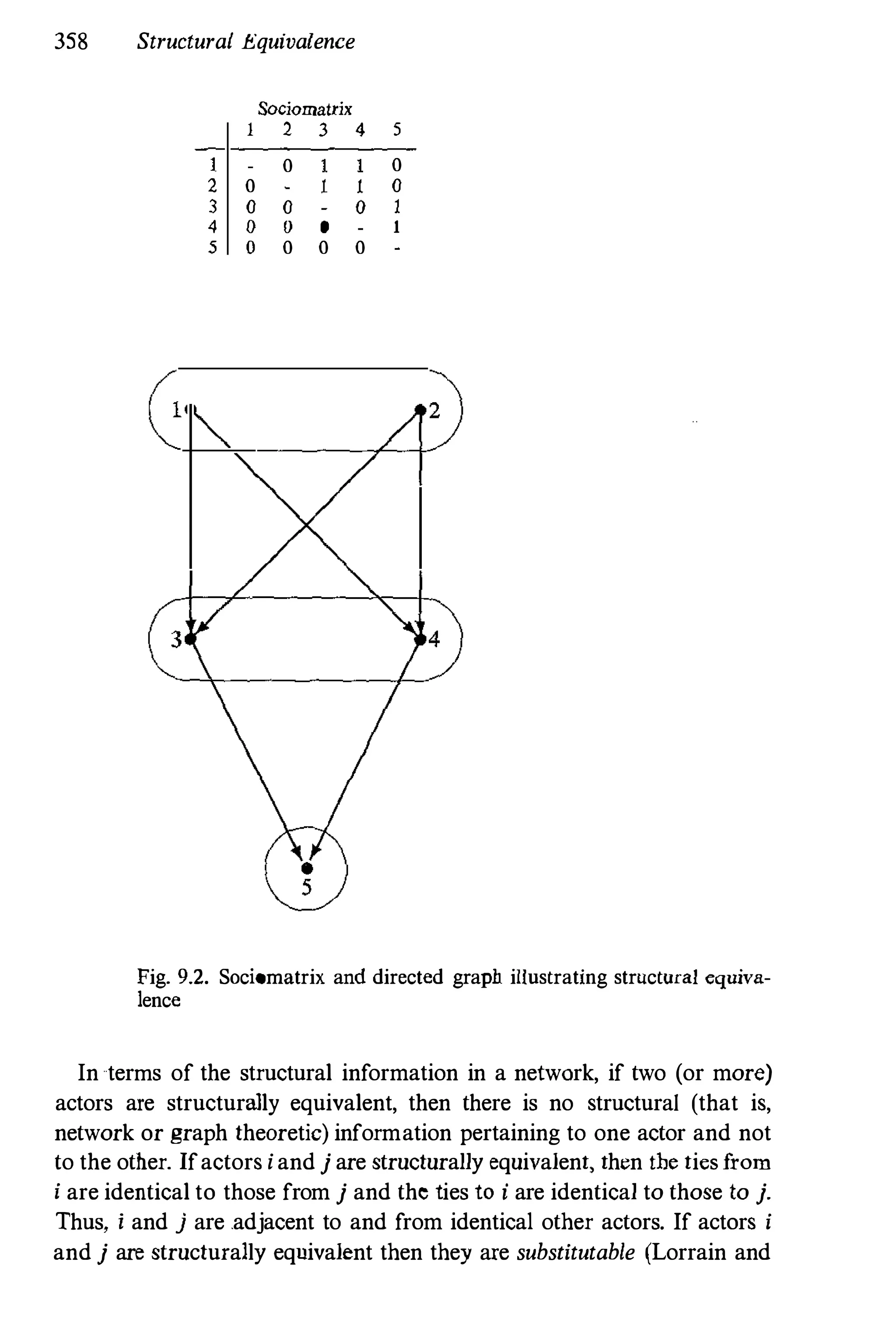
9.2 Sociomatrix and directed graph illustrating structural
equivalence 358
9.3 Example simplifying a network using structural equiva-
lence 364
9A Euclidean distances computed on advice relation for
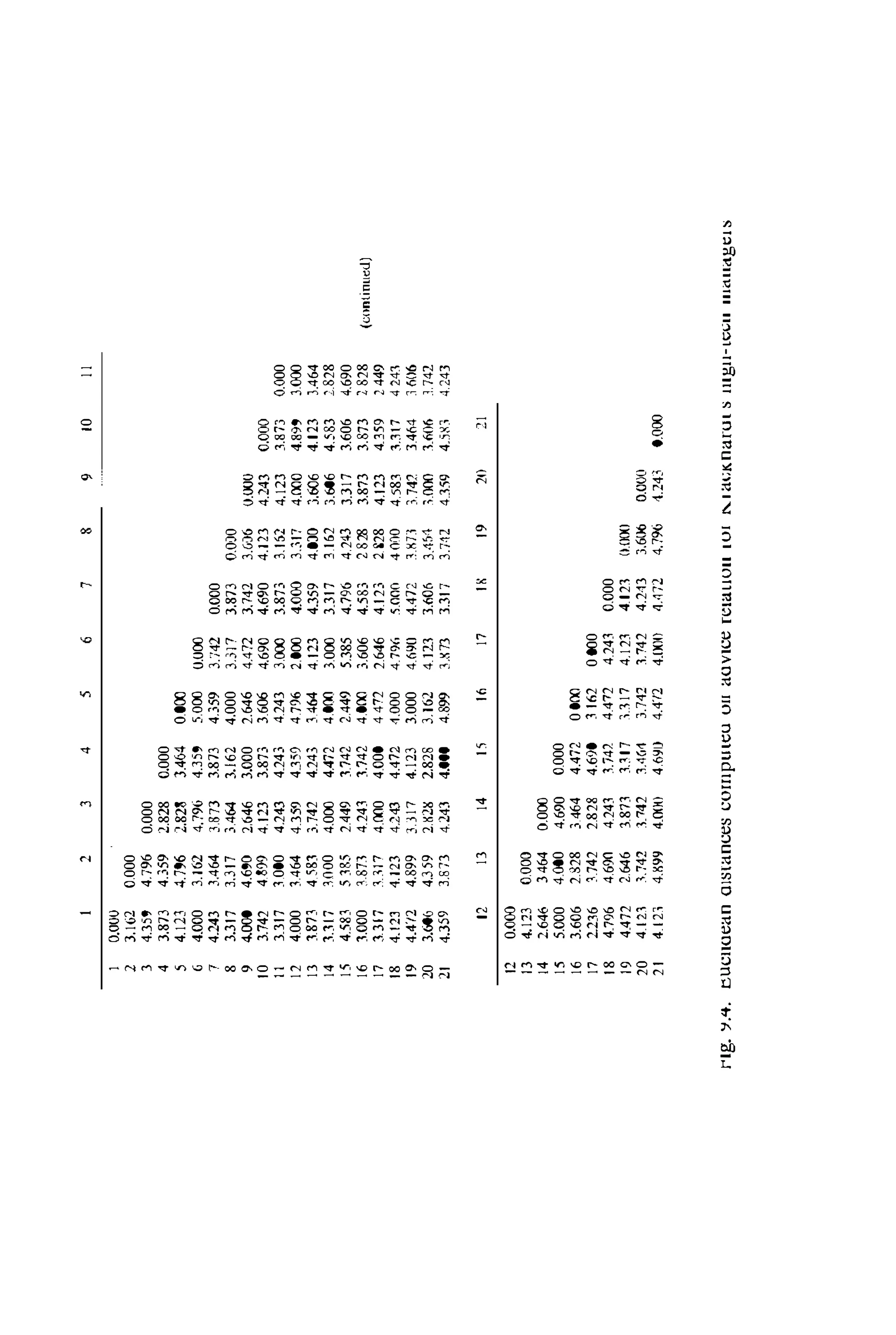
Krackhardt's high-tech managers 372
9.5 Correlations calculated on the advice relation for Krack-
hardt's high-tech managers 373
9.6 Dendrogram of positions from CONCOR of the advice
relation for Krackhardt's high-tech managers 379
9.7 Dendrogram for complete link hierarchical clustering of
Euclidean distances on.the advice relation for Krackhardt's
high-tech managers 383
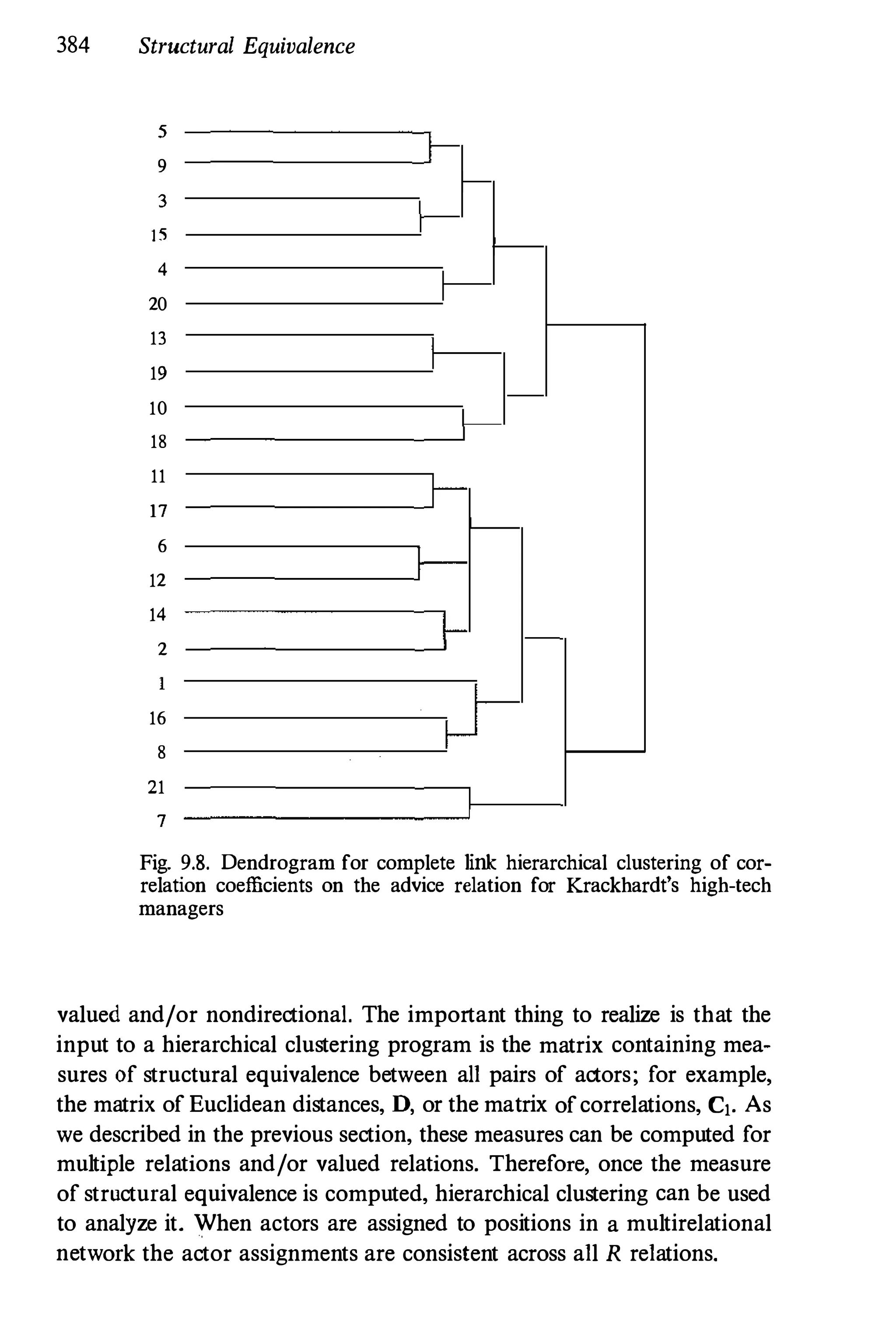
9.8 Dendrogram for complete link hierarchical clustering
of correlation coefficients on the advice relation for
Krackhardt's high-tech managers 384
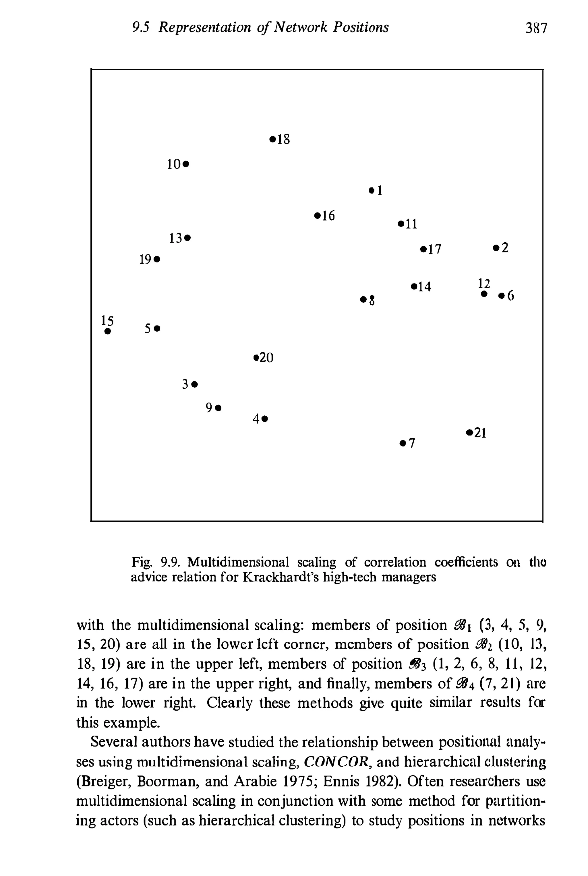
9.9 Multidimensional scaling of correlation coefficients on the
advice relation for Krackhardt's high-tech managers 387
9.10 Advice sociomatrix for Krackhardt's high-tech man-
agers permuted according to positions from hierarchical
clustering of correlations 389
9.11 Density table for the advice relation from Krackhardt's
high-tech managers, positions identified by hierarchical
clustering of correlations 390
9.12 Image matrix for the advice relation from Krackhardt's
high-tech managers, positions identified by hierarchical
clustering of correlations 390
9.13 Reduced graph for the advice relation from Krackhardt's
high-tech managers, positions identified by hierarchical
clustering of correlations 392
10.1 Density tables for advice and friendship relations for
Krackhardt's high-tech managers 403
10.2 Blockmodel image matrices for advice and friendship
relations for Krackhardt's high-tech managers 403
10.3 Reduced graphs for advice and friendship relations for
Krackhardt's high-tech managers 404
l OA Density tables for manufactured goods, raw materials, and
diplomatic ties· 405
List ofIllustrations xxvii
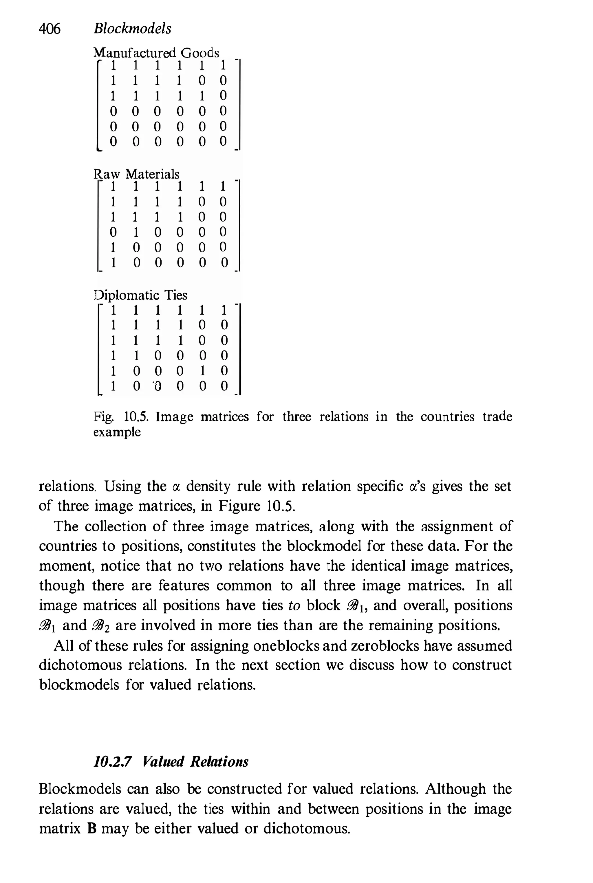
10.5 Image matrices for three relations in the countries trade
example 406
10.6 Frequency of ties within and between positions for advice
and friendship 416
10.7 Ten possible image matrices for a two-position blockmode1 421
10.8 Ideal images for blockmodels with more than two positions 423
11.1 Example of compound relations 431
11.2 Composition graph table for a hypothetical network 436
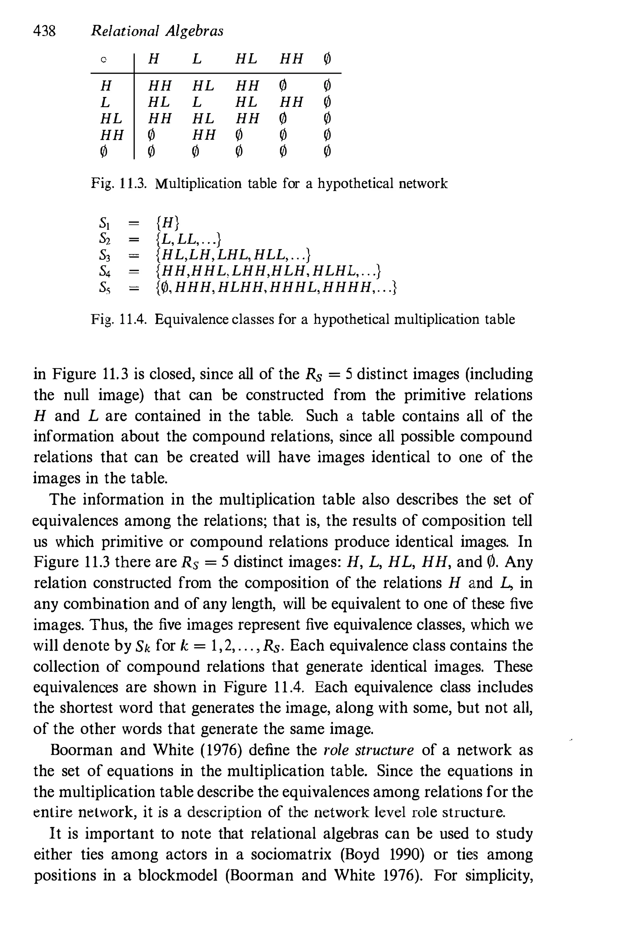
11.3 Multiplication table for a hypothetical network 438
11.4 Equivalence classes for a hypothetical multiplication table 438
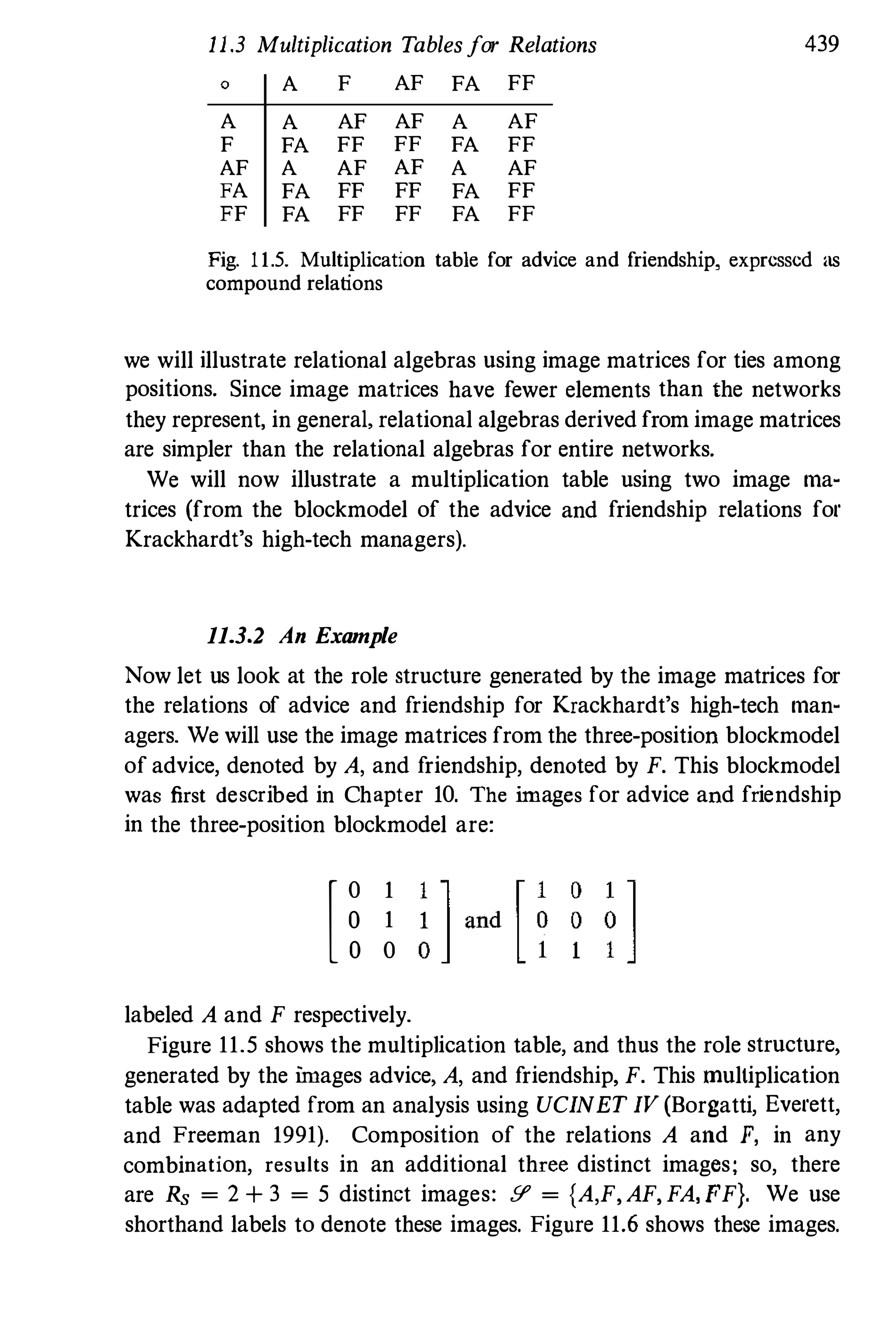
11.5 Multiplication table for advice and friendship, expressed
as compound relations 439
11.6 Image matrices for five distinct words formed from advice
and friendship images 440
11.7 Equivalence classes for multiplication role table of advice
and friendship 440
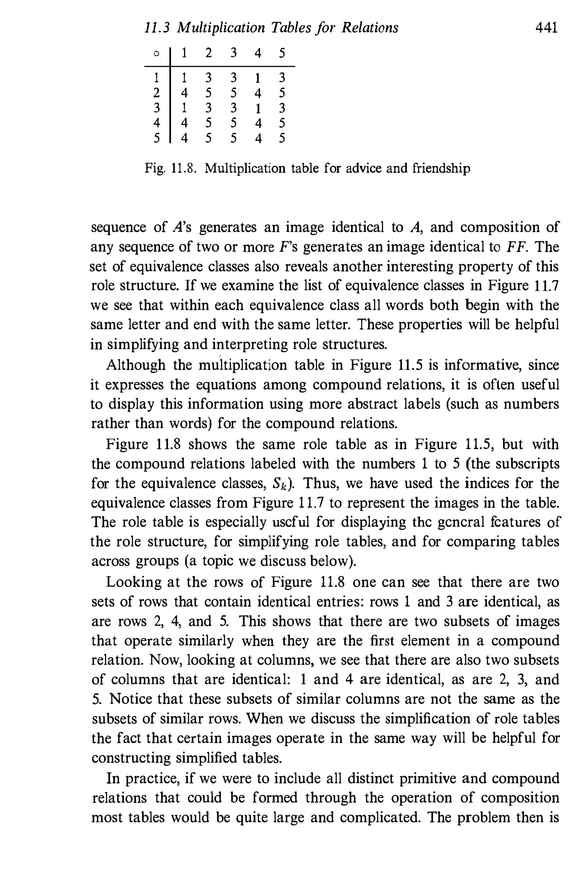
11.8 Multiplication table for advice and friendship 441
11.9 Inclusion ordering for the images from role structure of
advice and friendship 445
11.10 Permuted and partitioned multiplication table for advice
and friendship 446
11.11 Homomorphic reduction of the role table for advice and
friendship 447
11.12 A second permuted and partitioned multiplication table
for advice and friendship 448
11.13 A second homomorphic reduction of the role table for
advice and friendship 448
11.14 Multiplication table for helping (A) and friendship (F) for
the Bank Wiring room network 455
11.15 Permuted and partitioned multiplication table for helping
and friendship for the Bank Wiring room network 456
12.1 Graph to illustrate equivalences 468
12.2 Graph to demonstrate regular equivalence 476
12.3 Blocked sociomatrix and image matrix for regular
equivalence blockmodel 478
12.4 Regular equivalences computed using REGE on advice
and friendship relations for Krackhardt's high-tech
managers 482
12.5 Hierarchical clustering of regular equivalences on advice
and friendship for Krackhardt's high-tech managers 483
12.6 A hypothetical graph for two relations 486
12.7 Local roles 487
xxviii List ofIllustrations
12.8 Role equivalences for hypothetical example of two
relations 491
12.9 Role equivalences for advice and friendship relations for
Krackhardt's high-tech managers 492
12.10 Hierarchical clustering of role equivalences on advice and
friendship relations for Krackhardt's high-tech managers 493
12.11 Ego algebras for the example of two relations 497
. 12.12 Distances between ego algebras for a hypothetical example
of two relations 499
12.13 Distances between ego algebras computed on advice and
friendship relations for Krackhardt's high-tech managers 500
12.14 Hierarchical clustering of distances between ego algebras
on the two relations for Krackhardt's high-tech managers 501
13.1 The three dyadic isomorphism classes or states 511
13.2 The digraphs with the specified sets of outdegrees and
indegrees 551
14.1 Sociogram of friendship at the begiuning of the school
year for the hypothetical children network 560
14.2 Mutual/cyclic asymmetric triad involving children Allison
(nIl, Drew (n2), and Eliot (n3) 562
14.3 The six realizations of the single arc triad 563
14.4 The triad isomorphism classes (with standard MAN
labeling) 566
14.5 Transitive configurations 588
16.1 Plot of a, versus p, 713
16.2 Reduced graph based on predicted probabilities > 0.30 718
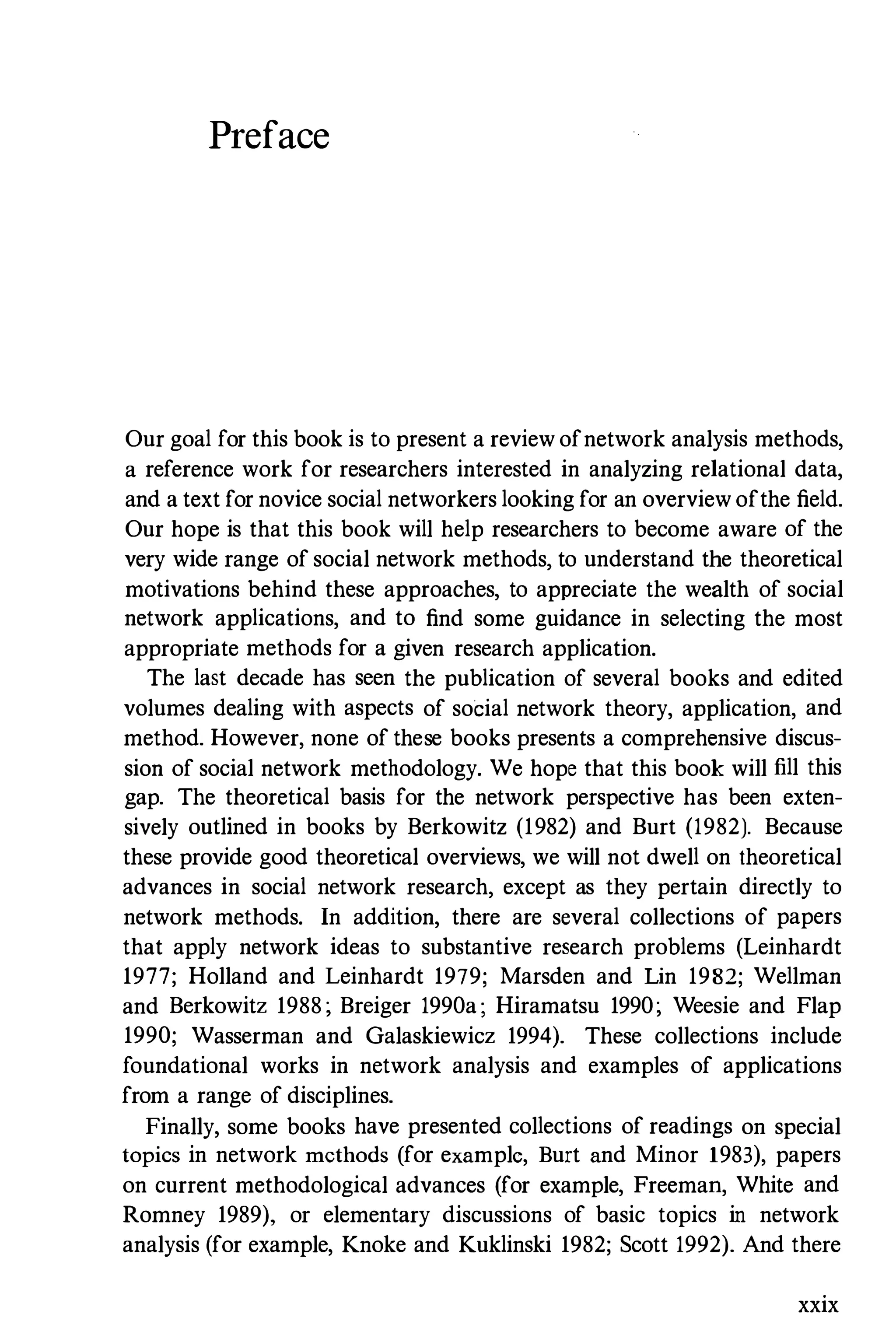
Preface
Our goal for this book is to present a review ofnetwork analysis methods,
a reference work for researchers interested in analyzing relational data,
and a text for novice social networkers looking for an overview ofthe field.
Our hope is that this book will help researchers to become aware of the
very wide range of social network methods, to understand the theoretical
motivations behind these approaches, to appreciate the wealth of social
network applications, and to find some guidance in selecting the most
appropriate methods for a given research application.
The last decade has seen the publication of several books and edited
volumes dealing with aspects of social network theory, application, and
method. However, none of these books presents a comprehensive discus­
sion of social network methodology. We hope that this book will fill this
gap. The theoretical basis for the network perspective has been exten­
sively outlined in books by Berkowitz (1982) and Burt (1982). Because
these provide good theoretical overviews, we will not dwell on theoretical
advances in social network research, except as they pertain directly to
network methods. In addition, there are several collections of papers
that apply network ideas to substantive research problems (Leinhardt
1977; Holland and Leinhardt 1979; Marsden and Lin 1982; Wellman
and Berkowitz 1988; Breiger 1990a; Hiramatsu 1990; Weesie and Flap
1990; Wasserman and Galaskiewicz 1994). These collections include
foundational works in network analysis and examples of applications
from a range of disciplines.
Finally, some books have presented collections of readings on special
topics in network methods (for example, Burt and Minor 1983), papers
on current methodological advances (for example, Freeman, White and
Romney 1989), or elementary discussions of basic topics in network
analysis (for example, Knoke and Kuklinski 1982; Scott 1992). And there
xxix
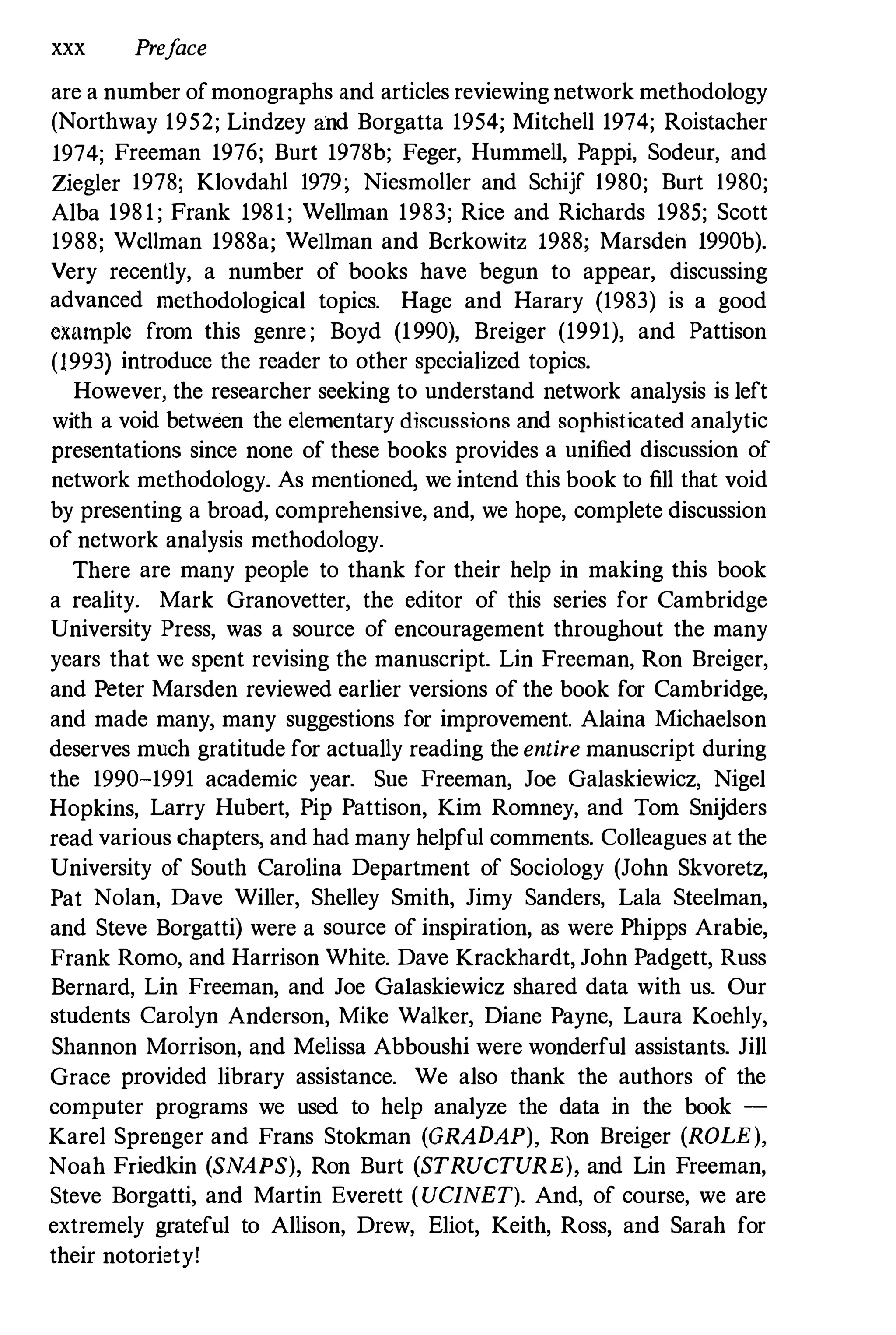
xxx Preface
are a nnmber ofmonographs and articles reviewing network methodology
(Northway 1952; Lindzey and Borgatta 1954; Mitchell 1974; Roistacher
1974; Freeman 1976; Burt 1978b; Feger, Hummell, Pappi, Sodeur, and
Ziegler 1978; Klovdahl 1979; Niesmoller and Schijf 1980; Burt 1980;
Alba 198 1 ; Frank 1981; Wellman 1983; Rice and Richards 1985; Scott
1988; Wc11man 1988a; WeHman and Berkowitz 1988; Marsden 1990b).
Very recently, a number of books have begun to appear, discussing
advanced methodological topics. Hage and Harary (1983) is a good
cxmnplc from this genre ; Boyd (1990), Breiger (1991), and Pattison
(1993) introduce the reader to other specialized topics.
However, the researcher seeking to understand network analysis is left
with a void between the elementary di�cussions and sophisticated analytic
presentations since none of these books provides a unified discussion of
network methodology. As mentioned, we intend this book to fill that void
by presenting a broad, comprehensive, and, we hope, complete discussion
of network analysis methodology.
There are many people to thank for their help in making this book
a reality. Mark Granovetter, the editor of this series for Cambridge
University Press, was a source of encouragement throughout the many
years that we spent revising the manuscript. Lin Freeman, Ron Breiger,
and Peter Marsden reviewed earlier versions of the book for Cambridge,
and made many, many suggestions for improvement. Alaina Michaelson
deserves much gratitude for actually reading the entire manuscript during
the 1990-1991 academic year. Sue Freeman, Joe Galaskiewicz, Nigel
Hopkins, Larry Hubert, Pip Pattison, Kim Romney, and Tom Snijders
read various chapters, and had many helpful comments. Colleagues at the
University of South Carolina Department of Sociology (John Skvoretz,
Pat Nolan, Dave Willer, Shelley Smith, Jimy Sanders, Lala Steelman,
and Steve Borgatti) were a source of inspiration, as were Phipps Arabie,
Frank Romo, and Harrison White. Dave Krackhardt, John Padgett, Russ
Bernard, Lin Freeman, and Joe Ga1askiewicz shared data with us. Our
students Carolyn Anderson, Mike Walker, Diane Payne, Laura Koehly,
Shannon Morrison, and Melissa Abboushi were wonderful assistants. Jill
Grace provided library assistance. We also thank the authors of the
computer programs we used to help analyze the data in the book -
Karel Sprenger and Frans Stokman (GRADAP), Ron Breiger (ROLE),
Noah Friedkin (SNAPS), Ron Burt (STRUCTURE), and Lin Freeman,
Steve Borgatti, and Martin Everett (UCINET). And, of course, we are
extremely grateful to Allison, Drew, Eliot, Keith, Ross, and Sarah for
their notoriety!
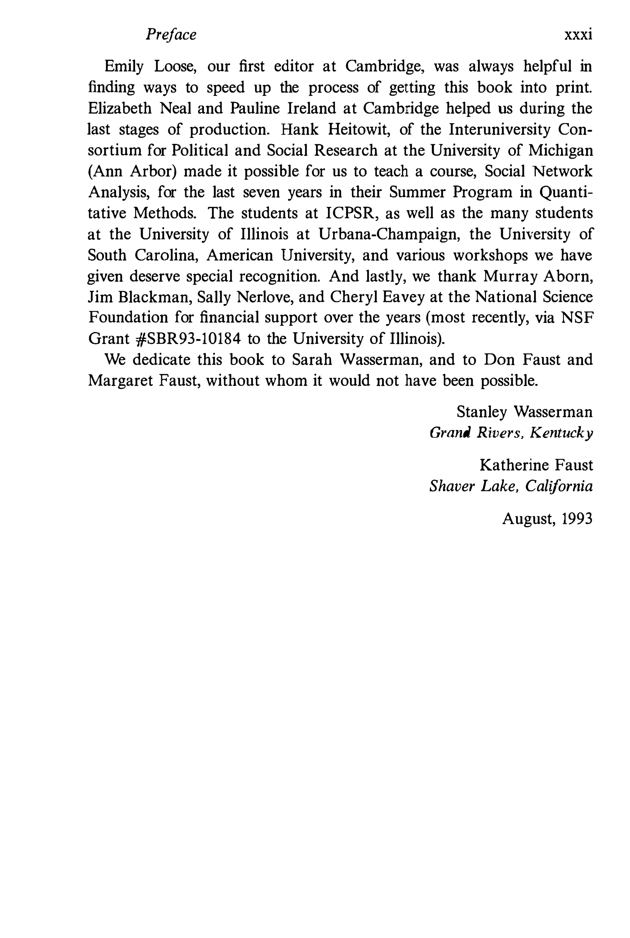
Preface xxxi
Emily Loose, our first editor at Cambridge, was always helpful in
finding ways to speed up the process of getting this book into print.
Elizabeth Neal and Pauline Ireland at Cambridge helped us during the
last stages of production. Hank Heitowit, of the Interuniversity Con­
sortium for Political and Social Research at the University of Michigan
(Ann Arbor) made it possible for us to teach a course, Social Network
Analysis, for the last seven years in their Summer Program in Quanti­
tative Methods. The students at ICPSR, as well as the many students
at the University of Illinois at Urbana-Champaign, the University of
South Carolina, American University, and various workshops we have
given deserve special recognition. And lastly, we thank Murray Aborn,
Jim Blackman, Sally Nedove, and Cheryl Eavey at the National Science
Foundation for financial support over the years (most recently, via NSF
Grant #SBR93-10184 to the University of Illinois).
We dedicate this book to Sarah Wasserman, and to Don Faust and
Margaret Faust, without whom it would not have been possible.
Stanley Wasserman
Grand Rivers, Kentucky
Katherine Faust
Shaver Lake, California
August, 1993
Part I
Networks, Relations, and Structure
1
Social Network Analysis in the
Social and Behavioral Sciences
The notion of a social network and the methods ofsocial network analy­
sis have attracted considerable interest and curiosity from the social and
behavioral science community in recent decades. Much of this interest
can be attributed to the appealing focus of social network analysis on
relationships among social entities, and on the patterns and implications
of these relationships. Many researchers have realized that the network
perspective allows new leverage for answering standard social and be­
havioral science research questions by giving precise formal definition
to aspects of the political, economic, or social structural environment.
From the view of social network analysis, the social environment can be
expressed as patterns or regularities in relationships among interacting
units. We will refer to the presence of regular patterns in relationship as
structure. Throughout this book, we will refer to quantities that measure
structure as structural variables. As the reader will see from the diversity
of examples that we discuss, the relationships may be of many sorts :
economic, political, interactional, or affective, to name but a few. The
focus on relations, and the patterns of relations, requires a set ofmethods
and analytic concepts that are distinct from the methods of traditional
statistics and data analysis. The concepts, methods, and applications of
social network analysis are the topic of this book.
The focus of this book is on methods and models for analyzing social
network data. To an extent perhaps unequaled in most other social
science disciplines, social network methods have developed over the past
fifty years as an integral part of advances in social theory, empirical
research, and formal mathematics and statistics. Many of the key struc­
tural measures and notions of social network analysis grew out of keen
insights of researchers seeking to describe empirical phenomena and are
motivated by central concepts in social theory. In addition, methods have
3
4 Social Network Analysis in the Social and Behavioral Sciences
developed to test specilic hypotheses about network structural properties
arising in the course of substantive research and model testing. The
result of this symbiotic relationship between theory and method is a
strong grounding of network analytic techniques in both application
and theory. In the following sections we review the history and theory
of social lIetwork analysis from the perspective of the development of
methodology.
Since our goal in this book is to provide a compendium of methods
lind applications for both veteran social network analysts, and for naive
but curious people from diverse research traditions, it is worth taking
some time at the outset to lay the foundations for the social network
perspective.
1.1 The Social Networks Perspective
In this section we introduce social network analysis as a distinct research
perspective within the social and behavioral sciences; distinct because
social network analysis is based on an aSllumption of the importance of
relationships among interacting units The social networR: perspective en­
compasses theories, models, and applications that are expressed in terms
ofrelational concepts or processes. That is relations defined by linkages
among umts are a fundamental component of network theories. Along
with growing interest and increased use of network analysis has come
a consensus about the central principles underlying the network per­
spective. These principles distinguish social network allalysis from other
research approaches (see Wellman 1988a, for example). In addition to
the use of relational concepts, we note the following as being important:
• Actors and their actions are viewed as interdependent rather
than independent, autonomous units
• Relational ties (linkages) between actors are channels for transfer
or "flow" of resources (either material or nonmaterial)
• Network models focusing on individuals view the network struc­
tural environment as providing opportunities for or constraints
on individual action
• Network models conceptualize structure (social, economic, polit­
ical, and so forth) as lasting patterns ofrelations among
,
actors
In this section we discuss these principles further and illustrate how
the social network perspective differs from alternative perspectives in
practice. Of critical importance for the development of methods for
},} The Social Networks Perspective 5
N"cial network analysis is the fact that the unitof analysis iu network
"nalysis is not the individual. but an entity consisting of a collection of
Individuals and the linkages among them, Network methods focus on
dynds (two actors and their ties), triads (three actors and their ties), or
Imgcr systems (subgroups of individuals, or entire networks), Therefore,
"pecial methods are necessary,
Formal Descriptions. Network analysis enters into the process
of model development, specification, and testing in a number of ways:
10 express relationally defined theoretical concepts by providing formal
definitions, measures and descriptions, to evaluate models and theories in
which key concepts and propositions are expressed as relational processes
orstructural outcomes, or to provide statistical analyses of multirelational
systems, In this first, descriptive context, network analysis provides
It vocabulary and set of formal definitions for expressing theoretical
concepts and properties, Examples of theoretical concepts (properties)
for which network analysis provides explicit definitions will be discussed
shortly.
Model and Theory Evaluation and Testing. Alternatively, net­
work models may be used to test theories about relational processes or
structures, Such theories posit specific structural outcomes which may
then be evaluated against observed network data, For example, suppose
one posits that tendencies toward reciprocation of support or exchange
of materials between families in a community should arise frequently.
Such a supposition can be tested by adopting a statistical model, and
studying how frequently such tendencies arise empirically,
The key feature of social network theories or propositions is that
they require concepts, definitions and processes in ",hich social units are
linked to one another by various relations. Both statistical and descriptive
uses of network analysis are distinct from more standard social science
analysis and require concepts and analytic procedures that are different
from traditional statistics and data analysis,
Some Background and Examples. The network perspective has
proved fruitful in a wide range ofsocial and behavioral science disciplines,
Many topics that have traditionally interested social scientists can be
thought of in relational or social network analytic terms. Some of the
topics that have been studied by network analysts are:
• Occupational mobility (Breiger 1981c, 1990a)
6 I'll/dol NI'/wol'k Analysis in the Social and Behavioral Sciences
il Th� Imp!ct of urbanization on individual well-being (Fischer
!<)�g,)
,. Tlw world political and economic system (Snyder and Kick 1979;
Nemeth and Smith 1985)
• Community elite decision making (Laumann, Marsden, and Ga­
laskiewicz 1977; Laumann and Pappi 1973)
• Social support (Gottlieb 1981; Lin, Woelfel, and Light 1986;
Kadushin 1966; Wellman, Carrington, and Hall 1988; Wellman
and Wortley 1990)
• Community (Wellman 1979)
• Group problem solving (Bavelas 1950; Bavelas and Barrett 1951;
Leavitt 1951)
• Diffusion and adoption of innovations (Coleman, Katz, and
Menzel 1957, 1966; Rogers 1979)
• Corporate interlocking (Levine 1972; Mintz and Schwartz 1981a,
1981b; Mizruchi and Schwartz 1987, and references)
• Belief systems (Erickson 1988)
• Cognition or social perception (Krackhardt 1987a; Freeman,
Romney, and Freeman 1987)
• Markets (Berkowitz 1988; Burt 1988b; White 1981, 1988; Leifer
and White 1987)
• Sociology of science (Mullins 1973; Mullins, Hargens, Hecht,
and Kick 1977; Crane 1972; Burt 1978j79a; Michaelson 1990,
1991 ; Doreian and Fararo 1985)
• Exchange and power (Cook and Emerson 1978; Cook, Emerson,
Gillmore, and Yamagishi 1983; Cook 1987; Markovsky, Willer,
and Patton 1988)
• Consensus and social influence (Friedkin 1986; Friedkin and
Cook 1990; Doreian 1981; Marsden 1990a)
• Coalition formation (Kapferer 1969; Thurman 1980; Zachary
1977)
The fundamental difference between a social network explanation and
a non-network explanation of a process is the inclusion of concepts
and information on relationships among units in a study. Theoretical
concepts are relational, pertinent data are relationa� and critical tests use
distributions of relational properties. Whether the model employed seeks
to understand individual action in the context of structured relationships,
or studies structures dIrectly, network analysis operationalIzes structures
in terms of networks oflInkages among units. Regularities or patterns in
1.1 The Social Networks Perspective 7
interactions give rise to structures. "Standard" social science perspectives
usually ignore the relational information.
Let us explore a couple of examples. Suppose we are interested in
corporate behavior in a large, metropolitan area, for example, the level
and types of monetary support given to local non-profit and charitable
organizations (see, for example, Galaskiewicz 1985). Standard social and
economic science approaches would first define a population of relevant
units (corporations), take a random sample of them (if the population
is quite large), and then measure a variety of characteristics (such as
size, industry, profitability, level of support for local charities or other
non-profit organizations, and so forth)..
The key assumption here is that the behavior of a specmc unit does
not influence any other units. However, network theorists take exception
to this assumption. It does not take much insight to realize that there
are many ways that corporations decide to do the things they do (such
as support non-profits with donations). Corporations (and other such
actors) tend to look at the behaviors of other actors, and even attempt
to mimic each other. In order to get a complete description of this
behavior, we must look at corporate to corporate relationships, such as
membership on each others' boards of directors, acquaintanceships of
corporate officers, joint business dealings, and other relational variables.
In brief, one needs a network perspective to fully understand and model
this phenomenon.
As another example, consider a social psychologist studying how
groups make decisions and reach consensus (Hastie, Penrod, and Pen­
nington 1983; Friedkin and Cook 1990; Davis 1973). The group might be
a jury trying to reach a verdict, or a committee trying to allocate funds.
Focusing just.on the outcome of this decision, as many researchers do,
is quite limiting. One really should look how members influence each
other in order to make a decision or fail to reach consensus. A network
approach to this study would look at interactions among group members
in order to better understand the decision-making process. The influences
a group member has on his/her fellow members are quite important to
the process. Ignoring these influences gives an incomplete picture.
The network perspective differs in fundamental ways from standard
social and behavioral science research and methods. Rather than fo­
cusing on attributes of autonomous individual units, the associations
among these attributes, or the. usefulness of one or more attributes for
predicting the level of auother attribute, the social network perspective
views characteristics of the social units as arising out of structural or
8 Social Network Analysis in the Social and Behavioral Sciences
relational processes or focuses on properties of the relational systems
themselves. The task is to understand properties of the social (economic
01' political) structural environment, and how these structural properties
inllucnce observed characteristics and associations among characteristics.
As Collins (1988) has so aptly pointed out in his review of network
theory.
Social life is relational; it's only because, say, blacks and whites occupy
particular kinds of patterns in networks in relation to each other that
"race" becomes an important variable. (page 413)
In social network analysis the observed attributes of social actors (such
as race or ethnicity of people, or size or productivity of collective bodies
such as corporations or nation-states) are understood in terms of patterns
or structures of ties among the units. Relational ties among actors are
primary and attributes of actors are secondary.
Employing a network perspective, one can also study patterns of rela­
tional structures directly without reference to attributes of the individuals
involved. For example, one could study patterns of trade among nations
to see whether or not the world economic system exhibits a cote-periphery
structure. Or, one could study friendships among high school students to
�ee whether or not patterns of friendships can be described as systems of
relatively exclusive cliques. Such analyses focus on characteristics of the
network as a whole and must be studied using social network concepts.
In the network analytic framework, the ties may be any relationship
existing between units; for example, kinship, material transactions, flow
of resources or support, behavioral interaction, group co-memberships,
or the afiective evaluation of one person by another. Clearly, some types
of ties will be relevant or measurable for some sorts of social units but
not for others. The relationship between a pair of units is a property
of the pair and not inherently a characteristic of the individual unit.
For example, the number (or dollar value) of Japanese manufactured
automobiles exported from Japan to the United States is part of the
trade relationship between Japan and the United States, and not an
intrinsic characteristic of either one country or the other. In sum, the
basic unit that these relational variables are measured on is the pair of
actors, not one or the other individual actors. It is important for methods
described in this book, that we assume that one has measurements on
interactions between all possible pairs of units (for example, trade among
all pairs of nations).
1.1 The Social Networks Perspective 9
It is important to contrast approaches in which networks and structural
properties are central with approaches that employ network ideas and
measurements in standard individual-level analyses. A common usage of
network ideas is to employ network measurements, or statistics calculated
from these network measurements, as variables measured at the individ­
ual actor level. These derived variables are then incorporated into a
more standard "cases by variables" analysis. For example, the range of a
person's social support network may be used as an actor-level variable in
an analysis predicting individual mental well-being (see Kadushin 1982),
or occupational status attainment (Lin and Durnin 1986; Lin, Ensel, and
Vaughn 1981; Lin, Vaughn, and Ensel 1981). We view analyses such as
these as auxiliary network studies. Network theories and measurements
become explanatory factors or variables in understanding individual be­
havior. We note that such an analysis still uses individual actors as the
basic modeling unit. Such analyses do not focus on the network structure
or network processes directly.
Our approach in this book is that network measurements are central.
We do not discuss how to use network measurements, statistics, model
parameter estimates, and so forth, in fnrther modeling endeavors. These
usual data analytic concerns are treated in existing standard statistics
and methods texts.
Tbe Perspective. Given a collection of actors, social network
analysis can be used to study the structural variables measured on actors
in the set. The relational structure of a group or -larger social system
consists of the pattern of relationships among the collection of actors.
The concept of a network emphasizes the fact that each individual has
ties to other individuals, each of whom in turn is tied to a few, some, or
many others, and so on. The phrase "social network" refers to the set
of actors and the ties among them. The network analyst would seek to
model these relationships to depict the structure of a group. One could
then study theimpact of this structure on the functioning of the group
and!or the influence of this structure on individuals within the group.
In the example of trade among nations, information on the imports
and exports among nations in the world reflects the global economic
system. Here the world economic system is evidenced in the observable
transactions (for example, trade, loans, foreign investment, or, perhaps,
diplomatic eXChange) among nations. The social network analyst could
then attempt to describe regularities or patterns in the world economic
system and to understand economic features of individual nations (such
10 Social Network Analysis in the Social and Behavioral Sciences
as rate of economic development) in terms of the nation's location in the
world economic system.
Network analysis can also be used to study the process of change
within a group over time. Thus, the network perspective also extends
longitudinally. For example, economic transactions between nations
could certainly be measnred at several points in time, thereby allowing a
researcher to use the network prespective to study changes in the world
economic system.
The social network perspective thus has a distinctive orientation in
which structures, their impact, and their evolution become the primary
focus. Since structures may be behavioral, social, political, or economic,
social network analysis thus allows a flexible set of concepts and methods
with broad interdisciplinary appeal.
1.2 Historical and Theoretical Foundations
Social network analysis is inherently an interdisciplinary endeavor. The
concepts ofsocial network analysis developed out ofa propitious meeting
of social theory and application, with formal mathematical, statistical,
and computing methodology. As Freeman (1984) and Marsden and
Laumann (1984) have documented, both the social sciences, and mathe­
matics and statistics have been left richer from the collaborative efforts
of researchers working across disciplines.
Further, and more importantly, the central concepts of relation, net­
work, and structure arose almost independently in several social and
behavioral science disciplines. The pioneers of social network analy­
sis came from sociology and social psychology (for example, Moreno,
Cartwright, Newcomb, Bavelas) and anthropology (Barnes, Mitchell). In
fact, many peol.'le attribute the first use of the term "social network " to
Barnes (1954). The notion of a network of relations linking social enti­
ties, or of webs or ties among social units emanating through society, has
found wide expression throughout the social sciences. Furthermore, many
of the structural principles of network analysis developed as researchers
tried to solve empirical and/or theoretical research puzzles. The fact
that so many researchers, from such different disciplines, almost simul­
taneously discovered the network perspective is not surprising. Its utility
is great, and the problems that can be answered with it are numerous,
spanning a broad range of disciplines.
In this section we briefly comment on the historical, empirical, and
theoretical bases of social network methodology. Some authors have
1.2 Historical and Theoretical Foundations 11
seen network analysis as a collection of analytic procedures that are
somewhat divorced from the main theoretical and empirical concerns of
social research. Perhaps a particular network method may appear to
lack theoretical focus because it can be applied to such a wide range of
substantive problems from many different contexts. In contras� we argue
that much network methodology arose as social scientists in a range
of disciplines struggled to make sense of empirical data and grappled
with theoretical issues. Therefore, network analysis, rather than being
an unrelated collection of methods, is grounded in important social
phenomena and theoretical concepts.
Social network analysis also provides a formal, conceptual means for
thinking about the social world. As Freeman (1984) has so convincingly
argued, the methods of social network analysis provide formal statements
about social properties and processes. Further, these concepts must
be defined in precise and consistent ways. Once these concepts have
been defined precisely, one can reason logically about the social world.
Freeman cites group and social role as two central ideas which, until
they were given formal definitions in network terms, could only serve as
"sensitizing concepts." The payoff of mathematical statements of social
concepts is the development of testable process models and explanatory
theories. We are in full agreement with Leinhardt's statement that "it
is not possible to build effective explanatory theories using metaphors"
(Leinhardt 1977, page xiv). We expand on this argument in the next
section.
1.2.1 Empirical Motivations
It is rare that a methodological technique is referred to as an "inven­
tion" but that is how Moreno described'his early 1930's invention, the
sociogram (Moreno 1953). This innovation, developed by Moreno along
with Jennings, marked the beginning of sociometry (the precursor to
social network analysis and much of social psychology). Starting at this
time point, this book summarizes over a half-century ofwork in network
analysis. There is wide agreement among social scientists that Moreno
was the founder of the field of sociometry - the measurement of inter­
personal relations in small groups - and the inspiration for the first two
decades of research into the structure of small groups. Driven by an inter­
est in understanding human social and psychological behavior, especially
group dynamics, Moreno was led to invent a means for depicting the in­
terpersonal structure of groups: the sociogram. A sociogram is a picture
12 Social Network Analysis in the Social and Behavioral Sciences
in which people (or more generally, any social units) are represented as
points in two-dimensional space, and relationships among pairs of peo­
ple are represented by lines linking the corresponding points. Moreno
claimed that "before the advent of sociometry no one knew what the
interpersonal structure of a group 'precisely' looked like" (1953, page Ivi).
This invention was revealed to the public in Apri1 1933 at a convention
of medical scholars, and was found to be so intriguing that the story was
immediately picked up by The New York Times (April 3, 1933, page 17),
and carried in newspapers across the United States. Moreno's interest
went far beyond mere depiction. It was this need to model important
social phenomena that led to two of the mainstays of social network
analysis : a visual display of group structure. and a probabilistic model
of structural outcomes.
Visual displays including sociograms and two or higher dimensional
representations continue to be widely used by network analysts (see Klov­
dahl 1986; Woelfel, Fink, Serota, Barnett, Holmes, Cody, Saltiel, Marlier,
and Gi11ham 1977). Two and sometimes three-dimensional spatial repre­
sentations (using multidimensional scaling) have proved quite useful for
presenting structures of influence among community elites (Laumann and
Pappi 1976; Laumann and Knoke 1987), corporate interlocks (Levine
1972), role structures in groups (Breiger, Boorman, and Arabie 1975;
Burt 1976, 1982), and interaction patterns in small groups (Romney and
Faust 1982; Freeman, Freeman, and Michaelson 1989).
Recognition that sociograms could be used to study social structure
led to a rapid introduction of analytic techniques. The history of this
development is nicely reviewed by Harary, Norman, and Cartwright
(1965), who themselves helped pioneer this development. At rhe same
time, methodologists discovered that matrices could be used to represent
social network data. These recognitions and discoveries brought the
power of mathematics to the study of social systems. Forsyth and Katz
(1946), Katz (1947), Lucc and Perry (1949), Bock and Husain (1950,
1952), and Harary and Norman (1953) were the first to use matrices in
novel methods for the study of social networks.
Other researchers also found inspiration for network ideas in the
course of empirical research. In the mid-1950's, anthropologists studying
urbanization (especially British anthropologists - such as Mitchell and
Barnes) found that the traditional approach of describing social organi­
zation in terms of institutions (economics, religion, politics, kinship, etc.)
was not sufficient for understanding the behavior of individuals in com­
plex societies (Barnes 1954; Bott 1957; Mitchell 1969; Boissevain 1968;
1.2 Historical and Theoretical Foundations 13
Kapferer 1969). Furthermore, as anthropologists turned their attention
to "complex" societies, they found that new concepts were necessary in
order to understand the fluid social interactions they observed in the
course of ethnographic field work (for example, see Barnes 1954, 1969a;
Boissevain 1968; also Mitchell 1969; and Boissevain and Mitchell 1973,
and papers therein). Barnes (1972), Whitten and Wolfe (1973), Mitchell
(1974), Wolfe (1978), Foster (1978/79), and others provide excellent re­
views of the history of social network ideas in anthropology. Many of
the current formal concepts in social network analysis, for example, den­
sity (Bott 1957), span (Thurman 1980), connectedness, clusterability, and
multiplexity (Kapferer 1969), were introduced in the 1950's and 1960's
as ways to describe properties of social structures and individual social
environments. Network analysis provided both a departure in theoretical
perspective and a way of talking about social phenomena which were
not easily defined using then current terminology.
Many social psychologists of the 1940's and 1950's found experimental
structures useful for studying group processes (Leavitt 1949, 195 1 ; Bave­
las 1948, 1950; Smith 1950; and many others; see Freeman, Roeder, and
Mulholland 1980, for a review). The experimentally designed communi­
cation structures employed by these researchers lent themselves naturally
to graphical representations using points to depict actors and lines to de­
pict channels of communication. Key insights from this research program
indicated that there were both important properties of group structures
and properties of individual positions within these structures. The theory
of the impact of structural arrangement on group problem solving and
individual performance required formal statements ofthe structural prop­
erties of these experimental arrangements. Structural properties found
by these researchers include the notions of actor centrality and group
centralization.
Clearly, important empirical tendencies led to important new, network
methods. Very important findings of tendencies toward reciprocity or
mutuality ofpositive affect, structural balance, and transitivity, discovered
early in network analysis, have had a profound impact on the study of
social structure. Bronfenbenner (1943) and Moreno and Jennings (1945)
were the first to study such tendencies quantitatively.
1.2.2 Theoretical Motivations
Theoretical notions have also provided impetus for development of net­
work methods. Here, we explore some of the theoretical concepts that
14 Social Network Analysis in the Social and Behavioral Sciences
have motivated the development of specific network analysis methods.
Among the important examples are : social group, isolate, popularity,
liaison, prestige, balance, transitivity, clique, subgroup, social cohesion,
social position, social role, reciprocity, mutuality, exchange, influence,
dominance, conformity. We briefly introduce some of these ideas below,
and discuss them all in more detail as they arise in later chapters.
Conceptions of social group have led to several related lines ofmethod­
ological development. Sociologists have used the phrase "social group"
in numerous and imprecise ways. Social network researchers have taken
specific aspects of the theoretical idea of social group to develop more
precise social network definitions. Among the more influential network
group ideas are: the graph theoretic entity of a clique and its general­
izations (Luce and Perry 1949; Alba 1973; Seidman and Foster 1978a;
Mokken 1979; and Freeman 1988); the notion of an interacting com­
munity (see Sailer and Gaulin 1984); and social circles and structures
of afliliation (Kadushin 1966 ; Feld 1981; Breiger 1974; Levine 1972;
McPherson 1982). The range and number of mathematical definitions of
"group" highlights the usefulness of using network concepts to specify
exact properties of theoretical concepts.
Another important theoretical concept, structural balance, was postu­
lated by Heider during the 1940's (Heider 1946), and later Newcomb
(1953). Balanced relations were quite common in empirical work; con­
sequently, theorists were quick to pose theories about why such things
occurred so frequently. This concept led to a very active thirty-year
period of empirical, theoretical, and quantitative research on triples of
individuals.
Balance theory was quantified by mathematicians using graph theoret­
ical concepts (Harary 1953, 1955b). Balance theory also influenced the
development of a large number of structural theories, including transitiv­
ity, another theory postulated at the level of a triple of individuals.
The related notions of social role. social status, and social position
have spawned a wide range of network analysis methods. Lorrain and
White were among the first social network analysts to express in social
network terms the notion of social role (Lorrain and White 1971). Their
foundational work on the mathematical property of structural equiva­
lence (individuals who have identical ties to and from all others in a
network) expressed the social concept of role in a formal mathematical
procedure. Much of the subsequent work on tltis topic has centered on
appropriate conceptualizations of notions of position (Burt 1976; Faust
1988; Borgatti and Everett 1992a) or role (White and Reitz 1983, 1989;
1.2 Historical and Theoretical Foundations 15
Winship and Mandel 1983; Breiger and Pattison 1986) in social network
terms.
1.2.3 Mathematical Motivations
Early in the theoretical development of social network analysis, re­
searchers found use for mathematical models. Beginning in the 1940's
with attempts to quantify tendencies toward reciprocity, social network
analysts have been frequent users and strong proponents of quantita­
tive analytical approaches. The three major mathematical foundations
of network methods are graph theory, statistical and probability theory,
and algebraic models. Early sociometricians discovered graph theory
and distributions for random graphs (for example, the work of Moreno,
Jennings, Criswell, Harary, and Cartwright). Mathematicians had long
been interested in graphs and distributions for graphs (see Erdos and
Renyi 1960, and references therein), and the more mathematical social
network analysts were quick to pick up models and methods from the
mathematicians. Graph theory provides both an appropriate representa­
tion of a social network and a set of concepts that can be used to study
formal properties of social networks.
Statistical theory became quite important as people began to study
reciprocity, mutuality, balance, and transitivity. Other researchers, par­
ticularly Katz and Powell (1955), proposed indices to measure tendencies
toward reciprocation.
Interest in rel:iprocity, and pairs of interacting individuals, led to a
focus on threesomes. Empirical and theoretical work on balance theory
and transitivity motivated a variety of mathematicians and statisticians
to formulate mathematical models for behavior of triples of actors.
Cartwright and Harary (1956) were the first to quantify structural balance
propositions, and along with Davis (1967), discussed which types oftriads
(triples of actors and all observed relational linkages among the actors)
should and should not arise in empirical research. Davis, Holland,
and Leinhardt, in a series of papers written in the 1970's, introduced a
wide variety of random directed graph distributions into social network
analysis, in order to test hypotheses about various structural tendencies.
During the 1980's, research on statistical models for social networks
heightened. Models now exist for analyzing a wide variety of social
network data Simple log linear models of dyadic interactions are now
commonly used in practice. These models are often based on Holland
and Leinhardt's (1981) Pl probability distribution for relational data.
16 Social Network Analysis in the Social and Behavioral Sciences
This model can be extended to dyadic interactions that are measured on
a nominal or an ordinal scale. Additional generalizations allow one to
simultaneously model multivariate relational networks. Network inter­
actions on different relations may be associated, and the interactions of
one relation with others allow one to study how associated the relational
variahles are. In the mid-1970's, there was much interest in models for the
study of networks over time. Mathematical models, both deterministic
and stochastic, are now quite abundant for such study.
Statistical models are used to test theoretical propositions about net­
works. These models allow the processes (which generate the data) to
show some error, or lack of fit, to proposed structural theories. One
can then compare data to the predictions generated by the theories to
determine whether or not the theories should be rejected.
Algebraic models have been widely used to study multirelational net­
works. These models use algebraic operations to study combinations of
relations (for example, "is a friend of," "goes to for advice," and "is a
friend of a friend") and have been used to study kinship systems (White
1963; Boyd 1969) and network role structures (Boorman and White 1976;
Breiger and Pattison 1986; Boyd 1990; and Pattison 1993).
Social network analysis attempts to solve analytical problems that
are non-standard. The data analyzed by network methods are quite
different from the data typically encountered in social and behavioral
sciences. In the traditional data analytic framework one assumes that
one has a set of measurements taken on a set of independent units
or case1S; thus giving rise to the familiar "cases by variables" data
array. The assumption of sampling independence of observations on
individual units allows the considerable machinery of statistical analysis
to be applied to a range ofresearch questions. However, social network
analysis is explicitly interested in the interrelatedness of social units. The
dependencies among the units are measured with structural variables.
Theories that incorporate network ideas are distinguished by propositions
about the relations among social units. Such theories argue that units
are not acting independently from one another, but rather influence each
other. Focusing on such structural variables opens up a different range
of possibilities for, and constraints on, data analysis and model building.
1.1.4 In Summary
The historical examination of empirical, theoretical, and mathematical
developments in network research should convince the reader that social
1.3 Fundamental Concepts in Network Analysis 17
network analysis is far more than an intuitively appealing vocabulary,
metaphor, or set of images for discussing social, behavioral, political,
or economic relationships. Social network analysis provides a precise
way to define important social concepts, a theoretical alternative to the
assumption of independent social actors, and a framework for testing
theories about structured social relationships.
The methods of network analysis provide explicit formal statements
and measures of social structural properties that might otherwise be de­
fined only in metaphorical terms. Such phrases as webs of relationships,
closely knit networks of relations, social role, social position, group,
clique, popularity, isolation, prestige, prominence, and so on are given
mathematical definitions by social network analysis. Explicit mathemat­
ical statements of structural properties, with agreed upon formal defini­
tions, force researchers to provide clear definitions of social concepts, and
facilitate development of testable models. Furthermore, network analysis
allows measurement of structures and systems which would be almost
impossible to describe without relational concepts, and provides tests of
hypotheses about these structural properties.
1.3 Fundamental Concepts in Network Analysis
There are several key concepts at the heart of network analysis that are
fundamental to the discussion of social networks. These concepts are:
actor, relational tie, dyad, triad, subgroup, group, relation, and network.
In this section, we define some of these key concepts and discuss the
different levels of analysis in social networks.
Actor. As we have stated above, social network analysis is con­
cerned with understanding the linkages among social entities and the
implications of these linkages. The social entities are referred to as ac­
tors.. Actors are discrete individual, corporate, or collective social units.
Examples of actors are people in a group, departments within a cor­
poration, public service agencies in a city, or nation-states in the world
system. Our use of the term "actor" does not imply that these entities
necessarily have volition or the ability to "act." Further, most social
network applications focus on collections actors that are all of the same
type (for example, people in a work group). We call such collections one­
mode networks. However, some methods allow one to look'at actors of
conceptually different types or levels, or from different sets. For example,
Galaskiewicz (1985) and Galaskiewicz and Wasserman (1989) analyzed
18 Social Network Analysis in the Social and Behavioral Sciences
monetary donations made from corporations to nonprofit agencies in the
Minneapolis/St. Paul area. Doreian and Woodard (1990) and Woodard
and Doreian (1990) studied community members' contacts with public
service agencies.
Relational Tie. Actors are linked to one another by social ties>
As we will see in the examples discussed throughout this book, the range
and type of ties can be quite extensive. The defining feature of a tie is
that it establishes a linkage between a pair of actors. Some of the more
common examples of ties employed in network analysis are:
• Evaluation of one person by another (for example expressed
friendship, liking, or respect)
• Transfers of material resources (for example business transac­
tions, lending or borrowing things)
• Association or affiliation (for example jointly attending a social
event, or belonging to the same social club)
• Behavioral interaction (talking together, sending messages)
• Movement between places or statuses (migration, social or phys­
ical mobility)
• Physical connection (a road, river, or bridge connecting two
points)
• Formal relations (for example authority)
• Biologicalrelationship (kinship or descent)
We will expand on these applications and provide concrete examples of
different kinds of ties in the discussion of network applications and data
in Chapter 2.
Dyad. At the most basic level, a linkage or relationship estab­
lishes a tie between two actors. The tie is inherently a property of the
pair and therefore is not thought of as pertaining simply to an individual
actor. Many kinds of network analysis are concerned with understand­
ing ties among pairs. All of these approaches take the dyad as the
unit of analysis. A dyad consists of a pair of actors and the (possible)
tie(s) between them. Dyadic analyses focus on the properties of pairwise
relationships, such as whether ties are reciprocated or not, or whether
specific types of multiple relationships tend to occur together. Dyads
are discussed in detail in Chapter 13, while dyadic statistical models are
discussed in Chapters 15 and 16. As we will see, the dyad is frequently
the basic unit for the statistical analysis of social networks.
1.3 Fundamental Concepts in Network Analysis 19
Triad. Relationships among larger subsets of actors may also be
studied. Many important social network methods and models focus on
the triad; a subset of three actors and the (possible) tie(s) among them.
The analytical shift from pairs of individuals to triads (which consist of
three potential pairings) was a crucial one for the theorist Simmel, who
wrote in 1908 that
. . .the fact that two elements [in a triad] are each connected not only
by a straight line - the shortest - but also by a broken line, as it were,
is an enrichment from a formal-sociological standpoint. (page 135)
Balance theory has informed and motivated many triadic analyses. Of
particular interest are whether the triad is transitive (if actor i "likes"
actor j, and actor j in turn "likes" actor k, then actor i will also «like"
actor k), and whether the triad is balanced (if actors i and j like each
other, then i and j should be similar in their evaluation of a third actor,
k, and if i and j dislike each other, then they should differ in their
evaluation of a third actor, k).
Subgroup. Dyads are pairs of actors and associated ties, triads
are triples of actors and associated ties. It follows that we can define
a subgroup of actors as any subset of actors, and all ties among them.
Locatiug and studying subgroups using specific criteria has been an
important concern in social network analysis.
Group. Network analysis is not simply concerned with collec­
lions of dyads, or triads, or subgroups. To a large extent, the power
of network analysis lies in the ability to model the relationships among
systems of actors. A system consists of ties among members of some
(more or less bounded) group. The notion of group has been given a
wide range of definitions by social scientists. For our purposes, a group
is the collection of all actors on which ties are to be measured. One
m.ust be able to argue by theoretical, empirical, or conceptual criteria
that the actors in the group belong together in a more or less bounded
set. Inde€d,. once one decides to gather data on a group, a more concrete
meaning of the term is necessary. A group, then, consists of a finite set of
actors who for conceptual, theoretical, or empirical reasons are treated
as a finite set of individuals on which network measurements are made.
The restriction to afinite set or sets ofactors is an ana1ytic requirement.
Though one could conceive of ties extending among actors in a nearly
infinite group of actors, one would have great difficulty analyzing data
on such a network. Modeling finite groups presents some of the more
20 Social Network Analysis in the Social and Behavioral Sciences
problematic issues in network analysis, including the specification of
network boundaries, sampling, and the definition of group. Network
sampling and boundary specification are important is
·
sues.
Early network researchers clearly recognized extensive ties among in­
dividuals (de Sola Pool and Kochen 1978; see Kochen 1989 for recent
work on this topic). Indeed, some early social network research looked
at the "smull world" phenomenon: webs and chains of connections ema­
nating to and from an individual, extending throughout the larger society
(Milgram 1967; Killworth and Bernard 1978).
However, in research applications we are usually forced to look at finite
collections of actors and ties between them. This necessitates drawing
some boundaries or limits for inclusion. Most network applications are
limited to a single (more or less bounded) group; however, we could
study two or more groups.
Throughout the book, we will refer to the entire collection of actors
on which we take measurements as the actor set. A network can contain
many groups of actors, but only one (if it is a one-mode network) actor
set.
Relation. The collection ofties ofa specific kind among members
of a group is called a relation. For example, the set offriendships among
pairs of children in a classroom, or the set of formal diplomatic ties
maintained by pairs of nations in the world, are ties that define relations.
For any group of actors, we might measure several different relations
(for example, in addition to formal diplomatic ties among nations, we
might also record the dollar amount of trade in a given year). It is
important to note that a relation refers to the collection ofties of a given
kind measured on pairs of actors from a specified actor set. The ties
themselves only exist between specific pairs of actors.
Social Network. Having defined actor, group, and relation we
can now give a more explicit definition ofsocial network. A social network
consists ofa finite set or sets ofactors and therelation orrelations defined
on them. The presence of relational information is a cntical and defining
feature of a social network. A much more mathematical definition of a
social network, but consistent with the simple notion given here, can be
found at the end of Chapter 3.
In Summary. These terms provide a core working vocabulary
for discussing social networks and social network data. We can see that
1.4 Distinctive Features 21
social network analysis not only requires a specialized vocabulary, but
also deals with conceptual entities and research problems that are quite
difficult to pursue using a more traditional statistical and data analytic
framework.
We now turn to some of the distinctive features of network analysis.
1.4 Distinctive Features of Network Theory and Measurement
It is quite important to note the key features that distinguish network
theory, and consequently network measurement, from the more usual
data analytic framework common in the social and behavioral sciences.
Such features provide the necessary motivation for the topics discussed
in this book.
The most basic feature ofnetwork measurement, distinctive from other
perspectives, is the use of structural or relational infonnation to study or
. test theories. Many network analysis methods provide formal definitions
and descriptions ofstructural properties ofactors, subgroups ofactors, or
groups. These methods translate core concepts in social and behavioral
theories into fonnal definitions expressed in relational terms. All of these
concepts are quantified by considering the relations measured among the
actors in a network.
Because network measurements give rise to data that are unlike other
social and behavioral science data, an entire body of methods has been
developed for their analysis. Social network data require measurements
on ties among social units (or actors); however, attributes of the actors
may also be collected. Such data sets need social network methods for
analysis. One cannot use mUltiple regression, t-tests, canonical correla­
tions, structural equation models, and so forth, to study social network
data or to test network theories. This book exists to organize, present,
critique, and demonstrate the large body of methods for social network
analysis.
Social network analysis may be viewed as a broadening or general­
ization of standard data analytic techniques and applied statistics which
usually focus on observational units and their characteristics. A social
network analysis must consider data on ties among the units. However,
attributes of the actors may also be included.
Measurements on actors will be referred to as network composition.
Complex network data sets may contain information about the charac­
teristics of the actors (such as the gender of people in a group, or the
GNP of nations in the world), as well as structural variables. Thus, the
22 Social Network Analysis in the Social and Behavioral Sciences
sort of data most often analyzed in the social and behavioral sciences
(cases and variables) may also be incorporated into network models. But
the fact that one has not only structural, but also compositional, vari­
ables can lead to very complicated data sets that can be approached only
with sophisticated graph theoretic, algebraic, and/or statistical methods.
Social network theories require specification in terms of patterns of
rclations, characterizing a group or social system as a whole. Given ap­
propriate network measurements, these theories may be stated as propo­
sitions about group relational structure. Network analysis then provides a
collection ofdescriptive procedures to determine how the system behaves,
and statistical methods to test the appropriateness of the propositions.
In contrast, approaches that do not include network measurements are
unable to study and/or test such theories about structural properties.
Network theories can pertain to units at different levels ofaggregation:
individual actors, dyads, triads, subgroups, and groups. Network analysis
provides methods to study structural properties and to test theories
stated at all of these levels. The network perspective, the theories, and
the measurements they spawn are thus quite wide-ranging. This is quite
unique in the social and behavioral sciences. Rarely does a standard
theory lead to theoretical statements and hence measurements at more
than a single level.
1.5 Organization of the Book and How to Read It
The question now is how to make sense of the more than 700 pages
sitting in front of you. First, find a comfortable chair with good reading
light (shoo the cats, dogs, and children away, if necessary). Next, make
sure your cup of coffee (or glass of scotch, depending on the time of
day) is close at hand, put a nice jazz recording on the stereo, and have
a pencil or highlighting pen available (there are many interesting points
throughout the book, and we are sure you will want to make note of
them).
This book is organized to highlight several themes in network analysis,
and to be accessible to readers with different interests and sophistication
in social network analysis. We have mentioned these themes throughout
this chapter, and now describe how these themes help to organize the
methods discussed in this book. These themes are:
• The complexity of the methods
• Descriptive versus statistical methods
1.5 Organization ofthe Book and How to Read It 23
• The theoretical motivation for the methods
• The chronological development of the methods
• The level of analysis to which the methods are appropriate
Since social network analysis is a broad, diverse, and theoretically varied
field, with a long and rich history, it is impossible to reflect all of these
possible thematic organizations simultaneously. However, insofar as is
practical and useful, we have tried to use these themes in the organization
of the book.
1.5.1 Complexity
First, the material progresses from simple to complex. The remainder
of Part I reviews applications of network analysis, gives an overview of
network analysis methods in a general way, and then presents notation
to be used throughout the book. Part II presents graph theory, develops
the vocabulary and concepts thaLare widely used in network analysis,
and relies heavily on examples. It also discusses simple actor and group
properties. Parts II, III, and IV require familiarity with algebra, and a
willingness to learn some graph theory (presented in Chapter 4). Parts V
and VI require some knowledge of statistical theory. Log linear models
for dyadic probabilities provide the basis for many of the techniques
presented later in these chapters.
1.5.2 Descriptive and Statistical Methods
Network methods can be dichotomized into those that are descriptive
versus those that are based on probabilistic assumptions. This dichotomy
is an important organizational categorization of the methods that we
discuss. Parts II, III, and IV of the book are based on the former.
The methods presented in these three parts of the book assume specific
descriptive models for the structure of a network, and primarily present
descriptive techniques for network analysis which translate theoretical
concepts.into formal measures.
Parts V and VI are primarily concerned with methods for testing
network theories and with statistical models of structural properties. In
contrast to a descriptive approach, we can also begin with stochastic
assumptions about actor behavior. Such models assume that there is
some probabilistic mechanism (even as simple as flipping a coin) that
underlies observed, network data. For example, one can focus on dyadic
24 Social Netwo/'" Analysis in the Social and Behavioral Sciences
interactions, and test whether an observed network has a specified amount
of reciprocity in the ties among the actors. Such a test uses standard
statistical theory, and thus one can formally propose a null hypothesis
which can then be rejected or not. Much of Chapter 13 is devoted
to a description of these mechanisms, which are then used throughout
Chaptet's 14, 15, and 16.
1.5.3 Theory Driven Methods
As we have discussed here, many social network methods were developed
by researchers in the course of empirical investigation and the develop­
ment oftheories. This categorization is one of the most important ofthe
book.
Part III covers approaches to groups and subgroups, notably cliques
and their generalizations. Sociological tendencies such as cohesion and
influence, which can cause actors to be "clustered" into subgroups, are
among the topics of Chapters 7 and 8. Part IV discusses approaches
related to the sociological notions of social role, status and position, and
the mathematical property of structural equivalence and its generaliza­
tions. The later sections of the book present statistical methods for the
analysis of social networks, many of which are motivated by theoretical
concerns. Part V covers models for dyadic and triadic structure, early
sociometry and social psychology of affective relations (dyadic analyses
of Chapter 13), and structural balance and transitivity (triadic analyses
of Chapters 6 and 14).
1.5.4 Chronology
It happens that the chapters in this book are approximately chronological.
The important empirical investigations of social networks began over
sixty years ago, starting with the sociometry of Moreno. This research
led to the introduction of graph theory (Chapter 4) to study structural
properties in the late 1940's and 1950's, and methods for subgroups
and cliques (Chapter 7), as well as structural balance and transitivity
(Chapters 6 and 14). More recently, H. White and his collaborators,
using the sociological ideas of formal role analysis (Nadel aud Lorrain),
introduced structural equivalence (Chapter 9), and an assortment of
related methods, in the 1970's, which in the 1980's, led to a collection of
algebraic network methods (Chapters 11 and 12).
1.5 Organization ofthe Book and How to Read It 25
As can be seen from our table of contents, we have mostly followed
this chronological order. We start with graph theory in Chapter 4, and
discuss descriptive methods in Parts III and IV before moving on to
the more recent statistical developments covered in Parts V and VI.
However, because of our interest in grouping together methods with
similar substantive and theoretical concerns, a few topics are out of
historical sequence (structural balance and triads in Chapters 6 and 14
for example). Thus, Part V (Dyadic and Triadic Methods) follows Part
IV (Roles and Positions). This reversal was made to place dyadic and
triadic methods next to the other statistical methods discussed in the
book (Part VI), since the methods for studying dyads and triads were
among the first statistical methods for networks.
1.5.5 Levels ofAnalysis
Network methods are usually appropriate for concepts at certain levels
of analysis. For example, there are properties and associated methods
pertaining just to the actors themselves. Examples include how "promi­
nent" an actor is within a group, as quantified by measures such as
centrality and prestige (Chapter 5), actor-level expansiveness and popu­
larity parameters embedded in stochastic models (Chapters 15 and 16),
and measures for individual roles, such as isolates, liaisons, bridges, and
so forth (Chapter 12). Then there are methods applicable to pairs of
actors and the ties between them, such as those from graph theory that
measure actor distance and reachability (Chapter 4), :structural and other
notions of equivalence (Chapters 9 and 12), dyadic analyses that postu­
late statistical models for the various states of a dyad (Chapter 13), and
stochastic tendencies toward reciprocity (Chapter 15). Triadic methods
are almost always based on theoretical statements about balance and
transitivity (Chapter 6), and postulate certain behaviors for triples of
actors and tbe ties among them (Chapter 14).
Many methods allow a researcher to find and study subsets of actors
that are homogeneous with respect to some network properties. Examples
of such applications include: cliques and other cohesive subgroups that
contain actors who are "close" to each other (Chapter 7), positions
of actors that arise via positional analysis (Chapters 9 and 10), and
subgroups ofactors that are assumed to behave similarly with respect to
certain model parameters arising from stochastic models (Chapter 16).
Lastly, there are measures and methods that focus on entire groups and
all ties. Graph theoretic measures such as connectedness and diameter
26 Social Network Analysis in the Social and Behavioral Sciences
(Chapter 4), group-level measures of centralization, density, and prestige
(Chapter 5), as well as blockmodels and role algebras (Chapters 9, 10,
and 11) are examples of group-level methods.
1.5.6 Chapter Prerequisites
Finally, it is important to note that some chapters are prerequisites for
others, while a number of chapters may be read without reading all
intervening chapters. This ordering ofchapters is presented in Figure 1.1.
A line in this figure connects two chapters if the earlier chapter contains
material that is necessary in order to read the later chapter. Chapters 1,
2, 3, and 4 contain the introductory material, and should be read before
all other chapters. These chapters discuss social network data, notation,
and graph theory.
From Chapter 4 there are five possible branches: Chapter 5 (cen­
trality); Chapter 6 (balance, clusterability, and transitivity); Chapter 7
(cohesive subgroups); Chapter 9 (structural equivalence); or Chapter 13
(dyads). Chapter 8 (affiliation networks) follows Chapter 7; Chapters 10
(blockmodels), 11 (relational algebras), and 12 (network role and posi­
tion) follow, in order, from Chapter 9; Chapter 15 (statistical analysis)
follows Chapter 13. Chapter 14 requires both Chapters 13 and 6. Chapter
16 (stochastic blockmodels and goodness-of-fit) requires both Chapters
15 and 10. Lastly, Chapter 17 concludes the book (and is an epilogue to
all branches).
A good overview of social network analysis (with an emphasis on
descriptive approaches including graph theory, centrality, balance and
clusterability, cohesive subgroups, structural equivalence, and dyadic
models) could include Chapters 1 through 10 plus Chapter 13. This ma­
terial could be covered in a one semester graduate course. Alternatively,
one could omit Chapter 8 and include Chapters 15 and 16, for a greater
emphasis on statistical approaches.
One additional comment - throughout the book, you will encounter
two symbols used to label sections: 0 and 0. The symbol 0 implies
that the text that follows is tangential to the rest of the chapter, and
can be omitted (except by the curious). The symbol 0 implies that the
text that follows requires more thought and perhaps more mathematical
and/or statistical knowledge than the other parts of the chapter, and
should be omitted (except by the brave).
1.6 Summary
1
!2
!3
!
5 �!�6
! ! !�!8 10 15 14
!�!11 16
!12
Fig. !.!. How to read this book
1.6 Summary
27
We have just described the history and motivations for social network
analysis. Network theories and empirical findings have been the primary
reasons for the development of much of the methodology described in
this book.
A complete reading of this book, beginning here and continuing on to
the discussion of network data in Chapter 2, then notation in Chapter
3, and so forth, should provide the reader with a knowledge of network
methods, theories, and histories. So without further ado, let us begin. . . .
2
Social Network Data : Collection and
Applications
This chapter discusses characteristics of social network data, with an
emphasis on how to collect such data sets. We categorize network data
in a variety of ways, and illustrate these categories with examples. We
also describe the data sets that we use throughout the book. As noted
in Chapter 1, the most important difference between social network
data and standard social and behavioral science data is that network
data include measurements on the relationships between social entities.
Most of the standard data collection procedures known to every social
scientist are appropriate for collecting network data (if properly applied),
but there are a few techniques that are specific to the investigation of
social networks. We highlight these similarities and differences in this
chapter.
2.1 Introduction: What Are Network Data?
Social network data consist of at least one structural variable measured
on a set of actors. The substantive concerns and theories motivating
a specific network study usually determine which variables to measure,
and often which techniques are most appropriate for their measurement.
For example, if one is studying economic transactions between countries,
one cannot (easily) rely on observational techniqnes; one would probably
use archival records to obtaiu informatiou ou such transactious. On
the other hand, friendships among people are most likely studied using
questionnaires or interviews, rather than using archival or historical
records. In addition, the nature of the study determines whether the
entire set of actors can be surveyed or whether a sample of the actors
must be taken.
28
2.1 Introduction: What Are Network Data? 29
The nature of the structural variables also determines which analytic
methods are appropriate for their study. Thus, it is crucial to understand
the nature of these variables. The data collection techniques described
here determine, to some degree, the characteristics of the relations.
2.1.1 Structural aud Composition Variables
There are two types of variables that can be included in a network data
set: structural and compositioil. Structural variables are measured on
pairs of actors (subsets of actors of size 2) and are the cornerstone of
social network data sets. Structural variables measure ties of a specific
kind between pairs of actors. For example, structural variables can
measurebusiness transactions between corporations, friendships between
people, or trade between nations. Actors comprising these pairs usually
belong to a single set of actors.
Composition variables are measurements of actor attributes. Compo­
sition variables, or actor attribute variables, are of the standard social
and behavioral science variety, and are defined at the level of individual
actors. For example, we ntight record gender, race, or ethnicity for peo­
ple, or geographical location, after-tax profits, or number of employees
for corporations. Some ofthe methods we discuss allow for simultaneous
analyses of structural and composition variables.
2.1.2 Modes
We will use the term "�ode" to refer to a distinct set of entities on
which the structural variables are measured (Tucker 1963, 1964, 1966;
Kroonenberg 1983; Arabie, Carroll, and DeSarbo 1987). Structural
variables measured on a single set of actors (for example, friendships
among residents of a neighborhood) give rise to one-mode networks.
The most common type of network is a one-mode network, since all
actors come from one set.
There are types of strnctural variables that are measured on two (or
even more) sets of entities. For example, we might study actors from
two different sets, one set consisting of corporations and a second set
consisting of non-profit organizations. We could then measure the flows
of financial support flows from corporations to non-profit actors. A
network data set containing two sets of actors is referred to as a two­
mode network, to reflect the fact that there are two sets of actors. A
two-mode network data set contains measurements on which actors from
30 Social Network Data
one of the sets have ties to actors in the other set. Usually, not all
. actors can initiate ties. Actors in one of the sets are "senders," while
those in the other are "receivers" (although the relation itself need not
be directional). We will consider one-mode and two-mode, and even
mention higher-mode, social networks in this book.
2.1.1 Affiliation Variables
A special type of two-mode network that arises in social network studies
is an affiliation network. Affiliation networks are two-mode, but have
only one set of actors. The second mode in an affiliation network is
a set of events (such as clubs or voluntary organizations) to which the
actors belong. Thus, in affiliation network data the two modes are the
actors and the events. In such data, the events are defined not on pairs
of actors, but on subsets of actors. These subsets can be of any size. A
subset ofactors affiliated with an affiliation variable is that collection of
actors who participate in a specific event, belong to a given club, and so
forth. Each affiliation variable is defined on a specific subset of actors.
For example, consider a set of actors, and three elite clubs in some city.
We can define an affiliation variable for each of these three clubs. Each
of these variables gives us a subset of actors - those actors belonging
to one of the clubs.
The collections of individuals affiliated with the events can be found
in a number of ways, depending on the substantive application. When
events are clubs, boards of directors of corporations, or committees, the
membership lists or rosters give the actors affiliated with each event.
Often events are informal social occasions, such as parties or other
gatherings, and observations or attendance or interactions among people
provide the affiliations ofthe actors (Bernard, Killworth, and Sailer 1980,
1982; Freeman and Romney 1987). One of the earliest, and now classic,
examples of an empirical application is the study of Davis, Gardner,
and Gardner (1941) of the cohesive subgroups apparent in the social
activities of women in a Southern city. Using newspaper records and
interviews, they recorded the attendance of eighteen women at fourteen
social events.
2.2 Boundary Specification and Sampling
A number of concerns arise in network studies that must be addressed
prior to gathering any network data. Typically, a researcher must first
2.2 Boundary Specification and Sampling 31
identify the population to be studied, and if sampling is necessary, worry
about how to sample actors and relations. These issues are considered
here.
2.2.1 What Is Your Population?
A very important concern in a social network study is which actors
to include. That is, who are the relevant actors? Which actors are in
the population? In the case of small, closed sets of actors (such as all
employees at a service station, faculty in an academic department, or
corporations headquartered in a major metropolitan area), this issue is
relatively easy to deal with. For other studies, the boundary of the set of
actors may be difficult (if not impossible) to determine. The boundary of
a set of actors allows a researcher to describe and identify the population
under study.
Actors may come and go, may be many in number and hard to
enumerate, or it may be difficult even to determine whether a specific
actor belongs in a set of actors. For example, consider the study of
elites in a community. The boundary of the set, including all, and
only, the elites within the community, may be difficult, or impossible, to
determine. However, frequently there will be a clear "external" definition
of the boundary of the set which enables the researcher to determine
which actors belong in it.
In some instances it is quite plausible to argue that a set of actors
is relatively bounded, as for example, when there is a fairly complete
membership roster. In such a case, the entire set of members can
make up the actor set. However, there are other instances when drawing
boundaries around a set is somewhat arbitrary. In practice, while network
researchers recognize that the social world consists of many (perhaps
infinite) links of connection, they also find that effective and reasonable
limits can be placed on inclusion. Network researchers often define actor
set boundaries based on the relative frequency ofinteraction, or intensity
of ties among members as contrasted with non-members.
Laumann, Marsden, and Prensky (1989) describe two different ap­
proaches to boundary specification in social network studies. The Iirst
way, which they refer to as the realist approach, focuses on actor set
boundaries and membership as perceived by the actors themselves. For
example, a street-corner gang is acknowledged as a social entity by its
members (it may even have a name - "Jets" or "Sharks") and the mem­
bership ofthe gang is the collection of people the members acknowledge
32 Social Network Data
as belonging to the gang. The second way of specifying network bound­
aries, which Laumann, Marsden, and Prensky refer to as the nominalist
approach, is based on the theoretical concerns of the researcher. For
example, a researcher might be interested in studying the flow computer
messages among researchers in a scientific specialty. In such a study, the
list of actors might be the collection of people who published papers on
the topic in the previous five years. This list is constructed for the ana­
lytical purposes of the researcher, even though the scientists themselves
might not perceive the list of people as constituting a distinctive social
entity. Both of these approaches to boundary specification have been
used in social network studies.
Consider now two specific examples of how researchers have defined
network boundaries. The first example illustrating the problem of iden­
tifying the relevant population of actors comes from a study of how
information or new ideas diffuse through a community. Coleman, Katz,
and Menzel (1957) studied how a new drug was adopted by physicians.
Their solution to the problem of boundary identification is as follows:
It was decided to include in the sample, as nearly as possible, all the
local doctors in whose specialities the new drug was of major potential
significance. This assured that the "others" named by each doctor in
answer to the sociometric questions were included in the sample. (page
254)
The second example comes from the study of community leaders by
Laumann and Pappi (1973). They asked community leaders to define the
boundary by identifYing the elite actors in the community ofAltneustadt.
These leaders were asked to
... name all persons [who] are now in general very influential in Alt­
neustadt.
From these lists, each ofwhich can be considered a sample ofthe relevant
actors in the elite network, the actor set was enumerated.
Many naturally occurring groups of actors do not have well-defined
boundaries. However, all methods must be applied to a specific set of
data which assumes not only finite actor set size(s), but also enumerable
set(s) of actors. Somehow, in order to study the network, we must
enumerate a finite set of actors to study.
For our purposes, the set of actors consists of all social �nits on which
we have measurements (either structural variables, or structural and com­
positional variables). Social network analysis begins with measurements
on a set ofactors. Researchers using methods described here must be able
2.2 Boundary Specification and Sampling 33
to make such an assumption. We assume, prior to any data gathering,
that we can obtain relevant information on all substantively important
actors; such actors will be included in the actor set. However, some actors
may be left out unintentionally or for other reasons. Thus, the constitu­
tion of the actor set (that is, its size and composition) depends on both
practical and theoretical concerns. The reason for the assumption that
the actor set consists of all social units on which we have measurements
is quite simple - the methods we discuss here cannot handle amorphous
set boundaries. We will always start our analyses with a set (or sets) of
actors, and we must be able to enumerate (or label) all members.
Many network studies focus on small collectivities, such as classrooms,
offices, social clubs, villages, and even, occasionally, artificially created
and manipulated laboratory groups. All of these examples have clearly
defined actor set boundaries; however, recent network studies of actors
such as elite business leaders in a community (Laumann and Pappi 1976),
interorganizational networks in a community (Galaskiewicz 1979, 1985;
Knoke 1983; Knoke and Wood 1981; Knoke and Kuklinski 1982), and
interorganizational networks across an entire nation (Levine 1972) have
less well-defined boundaries.
In several applications, when the boundary is unknown, special sam­
pling techniques such as snowball sampling (Goodman 1949, 1961; Er­
ickson 1978) and random nets (first proposed by Rapoport 1949a, 1949b,
1950, and especially 1963; recently resurrected by Fararo 1981, 1983, and
Fararo and Skvoretz 1984) can be used to define actor set boundaries.
Examples of social network studies using snowball sampling include:
Johnson (1990) and Johnson, Boster, and Holbert (1989) on commercial
fishermen; Moore (1979) and Alba and Moore (1978) on elite networks.
Such sampling techniques are discussed in the next section.
2.2.2 Sampling
Sometimes, it may not be possible to take measurements on all the actors
in the relevant actor set. In such situations, a sample of actors may be
taken from the set, and inferences made about the "popnlation" of actors
from the sample. Typically, the sampling mechanism is known, and the
sample is a good, probability sample (with known selection probabilities).
We will not assume in this book that the actors in the actor set(s)
are samples from some population. Most network studies focus on
well-defined, completely enumerated sets, rather than on samples of
actors from larger populations. Methodology for the latter situation is
34 Social Network Data
considerably different from methods for the former. With a sample, one
usually views the sample as representative of the larger, theoretically
interesting population (which must have a well-defined boundary and
hence, a known size), and uses the sampled actors and data to make
inferences about the population. For example, in a study of major
corporate actors in a national economy, a sample of corporations may
be taken in order to keep the size of the problem manageable; that is, it
might take too much time and/or too many resources actually to take a
census of this quite large population.
There is a large literature on network sampling, both applied and
theoretical. The primary focus of this literature is on the estimation of
network properties, such as the average number of ties per actor (see
Chapter 4), the degree of reciprocity present (see Chapter 13), the level
of transitivity (see Chapters 6 and 14), the density of the relation under
study (see Chapter 5), or the frequencies of ties between subgroups of
actors (see Chapter 7) based on the sampled units.
Frank (1977a, 1977b, 1977c, 1978b, 1979a, 1979b, 1980, 1985) is the
most widely known and most important researcher of sampling for social
networks. His classic work (Frank 1971) and more recent review papers
(Frank 1981, 1988) present the basic solutions to the problems that arise
when the entire actor set is not sampled. Erickson and Nosanchuk (1983)
review the problems that can arise with network sampling based on a
large-scale application of the standard procedures to a network of over
700 actors. Various other sampling models are discussed by Hayashi
(1958), Goodman (1961), Bloemena (1964), Proctor (1967, 1969, 1979),
Capobianco (1970), Sheardon (1970), and Cabobianco and Frank (1982).
One very clever network sampling idea originated with Goodman
(1961). A snowball network sample begins when the actors in a set
of sampled respondents report on the actors to whom they have ties
of a specific kind. All of these nominated actors constitute the "first­
order" zone of the network. The researcher then will sample all the
actors in this zone, and gather all the additional actors (those nominated
by the actors in the first-order zone who are not among the original
respondents or those in this zone). These additional actors constitute
the "second-order" zone. This snowballing proceeds through several
zones. Erickson (1978) and Frank (1979b) review snowball sampling,
with the goal of understanding how other "chain methods" (methods
designed to trace ties through a network from a source to an end; see,
for example, Granovetter 1974, and Useem 1973, for applications) can
be used in practice. Chain methods include snowball sampling and the
2.3 Types ofNetworks 35
small world technique discussed below. Erickson also discusses at length
the differences between standard network sampling and chain methods.
In some network sampling situations, it is not clear what the relevant
sampling unit should be. Should one sample actors, pairs of actors, triples
of actors, or perhaps even subsets of actors? Granovetter (1977a, 1977b)
and Morgan and Rytina (1977) have sensitized the network community to
these issues (see also Erickson, Nosanchuk, and Lee 1981, and Erickson
and Nosanchuk 1983). In other situations, one might sample actors,
and have them report on their ties and the ties that might exist among
the actors they choose or nominate. Such samples give rise to "ego­
centered" networks (defined later in this chapter). With a sample of
ego-centered networks, one usually wants to make inferences about the
entire population of such networks (see for example, the epidemiological
networks discussed by Klovdahl 1985; Laumann, Gagnon, Michaels,
Michael, and Coleman 1989; and Morris 1989, 1990). Statistically,
sampling dyads or ego-centered networks leads to sampling designs which
are not simple; the sampling is actually clustered, and one must adjust
the standard statistical summaries to allow for possible biases (Reitz and
Dow 1989).
2.3 Types of Networks
There are many different types of social networks that can be studied.
We will categorize networks by the nature of the sets of actors and
the properties of the ties among them. As mentioned earlier in this
chapter, we define the mode of a network as the number of sets of
entities on which structural variables are measured. One-mode networks,
the predominate type of network, study just a single set of actors, while
two-mode networks focus on two sets of actors, or one set of actors and
one set of events. One could even consider three- (and higher) mode
networks, but rarely have social network methods been designed for such
complicated data structures. Our discussion in this section is organized
by the number of modes in the network. We will first discuss one-mode
networks (with a single set of actors), then discuss two-mode networks,
first with two sets of actors and then with one set of actors and one set
of events. Applications of these three types of networks are the focus for
methods presented in this book.
The number of modes in a network refers to the number of distinct
kinds of social entities in the network. This usage is $lightly different from
the use of the term "mode" in the psychometric literature (Tucker 1964;
36 Social Network Data
Carroll and Arabie 1980). In that literature, mode refers to a "particular
class of entities" (Carroll and Arabie 1980, page 610). Thus, a study in
which subjects respond to a set of stimuli (such as questionnaire items)
gives rise to two modes: the subjects and the stimulus items. In the
standard sociometric data design, a number of actors are presented with
a list of the names of other people in the actor set, and asked to rate
each other person in terms of how much they "like" that person. In
a non-network context one could view these data as two-mode : the
people as respondents are the first mode, and the names of the people
as stimulus (questionnaire) items are the second mode. However, as a
social network, these data contain only a single set of actors, and thus,
in our terminology, it is a one-mode network in which the relation of
friendship is measured on a single set of people. One might very well be
interested in studying the set of respondents making evaluations of the
other people, in addition to studying the people as the "stimuli" that are
being evaluated. In that case one would consider respondents and stimuli
as two different modes (Feger and Bien 1982; Noma 1982b; Kumbasar,
Romney, and Batchelder n.d.).
We first categorize networks by how many modes the network has (one
or two), and by whether affiliational variables are measured. There are,
however, other kinds of relational data that are not one of these types.
One example is data arising from an ego-centered network design. Data
on such networks are gathered using special sampling strategies that
allow the researcher to focus on a specific set of respondents, and the
ties that these respondents have to particular others. We briefly describe
special ego-centered networks and special dyadic designs at the end of
this section.
We turn now to a discussion of one-mode, two-mode, and then affilia­
tional, and egocentric and special networks.
2.3.1 One-Mode Networks
Suppose the network under study is one-mode, and thus involves mea­
surements on just a single set of actors Consider first the nature of the
actors involved in such networks.
Actors. The actors themselves can be of a variety of types.
Specifically, the actors may be
• People
2.3 Types ofNetworks 37
• Subgroups
• Organizations
• Collectives/Aggregates:
- Communities
- Nation-states
Note that subgroups usually consist of people, organizations usually
consist of subgroups of people, while communities and nation-states are
larger entities, containing many organizations and subgroups. Thus,
there is a natural progression of types of actors from sets of people,
to collections or aggregates. Throughout this book, we will illustrate
methodology with examples consisting ofsocial network data on different
types of actors.
Relations. The relations measured on the single set of actors in a
one-mode network are usually viewed as representing specific substantive
connections, or "relational contents" (Knoke and Kuklinski 1982). These
connections, measured at the level of pairs of actors, can be ofmany types.
Barnes (1972) distinguishes, quite generally, between attitudes, roles, and
transactions. Knoke and Kuklinski (1982) give a more extensive list of
general kinds of relations. Specifically, the kinds of relations that we
might study include :
• Individual evaluations: friendship, liking, respect, and so forth
• Transactions or transfer of material resources: lending or bor­
rowing; buying or selling
• Transfer of non-material resources: communications, sending/
receiving information
• Interactions
• Movement: physical (migration from place-to-place), social
(movement between occupations or statuses)
• Formal roles
• Kinship: marriage, descent
One or more of these types of relations might be measured for a single
set of actors.
Individual evaluations are usually measurements of positive or negative
affect of one person for another. Sometimes, these relations are labeled
sentiment, and classically were the focus of the early sociometricians (see
Moreno 1934; Davis 1970; Davis and Leinhardt 1972). Without question,
such relations historically have been the most studied.
38 Social Network Data
Transactions, or transfers of material resources, include business trans­
actions, imports and exports of goods, specific forms of social support,
such as lending and borrowing, contacts made by one actor of another in
order to secure valuable resources, and transfer of goods. Such relations
include exchange of gifts, borrowing or lending items, and sales or pur­
chases (Galaskiewicz and Marsden 1978; Galaskiewicz 1979; Laumann,
Galaskiewicz, and Marsden 1978). Social support ties are also examples
of transactions (Wellman 1992b).
Transfers of non-material resources are frequently communications
between actors, where ties represent messages transmitted or information
received. These ties involve sending or receiving messages, giving or
receiving advice, passing on gossip, and providing novel information (Lin
1975; Rogers and Kincaid 1981; Granovetter 1974). Information about
innovations is frequently diffused over such communication channels
(Coleman, Katz, and Menzel 1966; Rogers 1979; Michaelson 1990).
Interactions involve the physical interaction of actors or their presence
in the same place at the same time. Examples of interactions include :
sittiog next to each other, attending the same party, visting a person's
home, hitting, hugging, disciplining, conversing, and so on.
Movement can also be studied using network data and processes.
Individuals moving between communities can be counted, as well as
workers changing jobs or people changing statuses (see, for example,
Breiger 1981c).
Formal roles, such as those dictated by power and authority, are also
relational Ties can represent authority of one actor over others, especially
in a management setting (White 1961). Example of formal roles include
boss/employee, teacher/student, doctor/patient, and so on.
Lastly, kinship relations have been studied using network methods for
many years. Ties can be based on marriage or descent relationships and
marriage or family relationships can be described using social network
methods (for example, see White 1963; Boyd 1969).
Actor Attributes. In addition to relational information, social
network data sets can contain measurements on the characteristics of
the actors. Such measurements of actor attribute variables constitute the
composition of the social network.
These variables have the same nature as those measured in non­
network studies. People can be queried about their age, gender, race,
socioeconomic status, place of residence, grade in school, and so on.
For corporate actors, one can measure their profitability, revenues, geo-
2.3 Types ofNetworks 39
graphical location, purpose of business, and so on. The "size, shape, and
flavor" of the actors constituting the network can be measured in many
ways.
2.3.2 Two-Mode Networks
Suppose now that the netwo.rk..under study is two-mode, and thus involves
measurements on two sets of actors, or on a set of actors and a set of
events. We will first consider the case in which relations are measured
on pairs of actors from two different actor sets. We will then discuss a
special kind of two-mode network in which measurements are taken on
subsets of actors.
Two Sets of Actors. Relations in a two-mode network measure
ties between the actors in one set and actors in a second set. We call such
networks dyadic two-mode networks, since these relations are functions
of dyads in which the first actor and the second actor in the dyad are
from different sets.
With respect to the different types of actors, the types of relations,
and the types of actor attribute variables, all of our discussion about
one-mode networks is relevant. Note, however, that there can be multiple
types ofactors, and we can have a unique collection of attribute variables
for each set of actors.
Actors. In a two-mode network that contains two sets of actors,
these actors can be of the general types as described for one-mode
networks. However, the two sets of actors may be of different types.
Relations. In a two-mode network with two sets of actors, at
least one relation is measured between actors in the two sets. In a more
extensive two-mode network data set, relations can also be defined on
actors within a set. However, for the network to be truly two-mode with
two sets of actors, at least one relation must be defined between the two
sets of actors.
An example of such a network can be found in Galaskiewicz and
Wasserman (1989). The data analyzed there consisted of two sets of
actors: a collection of corporations headquartered in the MinneapolisjSt.
Paul metropolitan area, and the non-profit organizations (such as the Red
Cross, United Way, public radio and television stations) which rely on
contributions from the public sector for their operating budgets. The
40 Social Network Data
primary relation was the flow of donations from the corporations to
the non-profit organizations, clearly a two-mode relation. Also, it is
important to note that this relation is unidirectional since it flows from
actors in one set to actors in the other set, but not the reverse. In addition,
the analysis by Galaskiewicz and Wasserman considered a number of
relations dcfined just for the corporations (such as shared country club
memberships among the chief executive officers) and several just for the
non-profits (such as interlocking boards of directors). A part of this data
set will be discussed in more detail later in this chapter.
One Set of Actors and One Set of Events. The next type of
two-mode social network, which we refer to as an affiliation network,
arises when one set of actors is measured with respect to attendance at,
or affiliation with, a set of events or activities. The first mode in an
affiliation network is a set of actors, and the second is a set of events
which affiliates the actors.
An example comes from Davis, Gardner, and Gardner (1941), as
described and analyzed by Homans (1950) and Breiger (1974). A set of
women attended a variety of social functions, and this attendance was
recorded over a period of several months. Each social function can be
viewed as a variable, and a binary measurement made as to whether a
specific actor attended the specific function. These variables are termed
affiliational. Such data and networks are called affiliation networks, or
sometimes, membership networks. And since the affiliations are measured
on subsets of actors, such networks are non-dyadic, two-mode networks.
Actors. In an affiliation network, we have a first set of actors,
and a second set of events or activities to which the actors in the first
set attend or belong. The types of actors in affiliation networks can be
exactly the same as those in one-mode and two-mode networks. The only
requirement is that the actors must be affiliated with one or more events.
Events. In affiliation networks, actors (the first mode) are related
to each other through theirjoint affiliation with events (the second mode).
The events are often defined on the basis of membership in clubs or
voluntary organizations (McPherson 1982), attendance at social events
(Davis, Gardner, and Gardner 1941), sitting on a board of directors, or
socializing in a small group (Bernard, Killworth, and Sailer 1980, 1982;
Wilson 1982).
2.3 Types ofNetworks 41
The nature of the events, which affiliate the actors, depends on the
type of actors involved. People may attend social functions or belong to
athletic clubs, subgroups of people may attend various committee meet­
ings (for example, departments at a major university send representatives
to college committee meetings), organizations may be represented on
various boards of directors in a community, or countries might belong
to treaty organizations� and so OD.
Attributes. We can have actor attribute variables that are of
the same types as those for one-mode and two-mode networks. In
addition, the events themselves may have characteristics associated with
them which can be measured and included in the network data set.
For example, clubs will be of a particular size or located in a specific
geographical area. Events usually occur at discrete points in time, as
well as in particular geographical places. Thus, there can be two sets of
attribute variables in an affiliation network data set: attributes of the
actors, and attributes of the events.
Methods for analyzing affiliation network data are described in Chap­
ter 8, and are applied to a network data set giving the memberships of
a set of chief executive officers of major corporations in Minneapolis/St.
Paul in a set of exclusive clubs.
2.3.3 Ego-centered and Special Dyadic Networks
Not all structural data give rise to standard social network data sets. With
standard network data (regardless of how many modes the network has),
one enumerates not only the actors, but the relevant pairs as well. All
actors (theoretically) can relate to each other in one-mode networks.
In two-mode networks with two sets of actors, all actors in the first
mode can (theoretically) relate to all in the second. However, some data
collection designs gather structural information on some pairs but not
others. An example of such data arises in studies of couples. Each partner
in the couple can interact with the other but with no other person during
counseling sessions. Interactions during these sessions are then recorded.
When interest centers on a collection of pairs (husband-wife, father-son,
and so forth), one frequently samples from a large population of such
pairs. We will refer to these non-network relational data as special dyadic
designs.
An actor may also relate to a limited number of "special" other
actors. For example, one might observe mothers interacting with their
42 Social Network Data
own children in an experimental situation. In this case, mothers only
interact with their own children, and children only interact with their
own mother. Thus, the partners for one person (either mother or child)
are different from the partners for another. In this situation, the design
of the experiment constrains the interactions among the set of people so
that all people cannot, theoretically, interact with all others.
Another related design is an ego-centered network. An ego-centered
network consists ofa focal actor, termed ego, as set ofalters who have ties
to ego, and measurements on the ties among these alters. For example,
when studying people, one samples respondents, and each respondent
reports on a set of alters to whom they are tied, and on the ties among
these alters. Such data are often referred to as personal network data.
Clearly these data are relational, but limited, since ties from each actor
are measured only to some (usually only a few) alters. For example,
in 1985 the General Social Survey conducted by the National Opinion
Research Center (see Burt 1984, 1985) asked respondents:
Looking back over the last six months � who are the people with
whom you discussed matters important to you? (1984, page 119)
Respondents also reported on the ties between the people they listed.
Bernard, Johnsen, Killworth, McCarty, Shelley, and Robinson (1990),
Killworth, Johnsen, Bernard, Shelley, and McCarty (1990), Huang and
Tausig (1990), Burt (1984, 1985), Marsden (1987, 1990b), Wellman (1993),
as well as Campbell. Marsden and Hurlbert (1986) discuss measurement
of such personal. ego-centered networks.
Ego-centered networks have been widely used by anthropologists to
study the social environment surrounding individuals (Boissevain 1973)
or families (Bott 1957). Ego-centered networks are also used quite often
in the study of social support. The term "social support" has been used
to refer to social relationsJiips that aid the health or well-being of an
individual. The emphasis on relationships has allowed researchers to
study support using social networks. Such networks are of great interest
in clinical and community psychology, as well as in sociology. A variety
of hypotheses (see Hammer 1983; Cohen and Syme 1985) have been
offered to explain how personal relationships, as reflected by such ego­
centered networks, can affect the emotional and physical well-being of
an individual.
The methods described in this book assume that there are no theo­
retical 1imitations on interactions among actors. A social network arises
when all actors can, theoretically, have ties to all relevant actors. The pri-
2.4 Network DatQ, Measurement and Collection 43
mary object of study for methods discussed in this book is this complete
collection of actors (one or more sets) and the ties among them.
2.4 Network Data, Measurement and Collection
We now turn to issues concerning the measurement and collection of
network data, the accuracy, validity, and error associated with these
data, and particular design considerations that can arise in network
studies.
2.4.1 Measurement
Social network data differ from standard social and behavioral science
data in a number of important ways. Most importantly, social network
data consist of one (or more) relations measured among a set of actors.
The presence of relations has implications for a number of measurement
issues, including the unit of observation (actor, pair of actors, relational
tie, or event), the modeling unit (the actor, dyad, triad. subset of ac­
tors, or network), and the quantification of the relations (directional vs.
nondirectional; dichotomous vs. valued). We will discuss each of these
issues in turn.
Social network data can be studied at a number of different levels: the
individual actor, the pair of actors or dyad, the triple of actors or triad,
a subset of actors, or the network as a whole. We will refer to the level
at which network data are studied as the modeling unit However, social
network data often are gatbered at a level that is different from the level
at which they are modeled. We discuss the unit of observation and the
modeling unit in the next two sections.
Unit of Observation. The unit of observation is the entity on
which measurements arc taken Most often social network data are
collected by observing, interviewing, or questioning individual actors
about the ties from these actors to other actors in the set. Thus, the unit
of observation is an actor, from whom we elicit information about ties.
The dyad is the unit of observation when one measures ties among pairs
of actors directly. For example, one could record instances of aggression
among pairs of children on a playground. When affiliation network data
are collected, the unit of observation is often the event. The researcher
selects events or social occasions, and for each event, records the actors
who are affiliated with it.
44 Social Network Data
Modeling Unit. Just as social network data can be observed at
a number of levels, there are several levels at which network data can be
modeled or summarized. These levels are the:
• Actor
• Dyad
• Triad
• Subgroup
• Set of actors or network
In categorizing network methods, it is useful to consider the level to which
a model or network property applies. Some network properties pertain
to actors (for example the number of "choices" that an individual actor
receives from others in the network). Other properties pertain to pairs
of actors (for example, if one person "chooses" another as a friend, is
the "choice" returned by the second person?). Models at the level of the
triad consider triples of actors and the ties among them. Many methods
pertain to subgroups of actors; for example, one could study whether
there are subsets of actors in the network who interact frequently with
each other. Finally many properties pertain to the network as a whole,
for example, the proportion of ties that are present in the network.
Relational Quantification. There are two properties of relations
that are important for understanding..their measurement. and for catego­
rizing the methods described here: whether the relation is directional or
nondirectional, and whether it is dichotomous or valued. In a directional
relation, the relational tie between a pair of actors has an origin and
a destination; that is, the tie is directed from one actor in the pair to
the other actor in a pair. For example, one country exports manufac­
tured goods to a second country; the first country is the source of the
manufactured goods, and the second country is the destination. In a
nondircctional relation the tie between a pair of actors does not have
a direction. For example, we could define a tie as present between two
countries if they share a border.
A second important property of a relation is whether it is dichotomous
or valued. Dichotomous relations are coded as either present or absent,
for each pair of actors. For example one could record whether one
country sends an ambassador to a second country; thus giving rise to
a dichotomous relation that can only take on two values : "send" or
"not send." On the other hand, valued relations can take on a range of
values, indicating the strength, intensity, or frequency of the tie between
2.4 Network Data, Measurement and Collection 45
each pair of actors. For example, we could record the dollar value of
manufactured goods that are exported from one country to a second
country, thus giving rise to a valued relation.
2.4.2 Collection
There are a variety of ways in which social network data can be gathered.
These techniques are:
• Questionnaires
• Interviews
• Observations
• Archival records
• Experiments
• Other techniques, including ego.centered, small world, and di·
aries
Each of these techniques will be discussed and illustrated with examples.
Questionnaire, This data collection method is the most com­
monly used (especially when actors are people). The questionnaire usu­
ally contains questions about the respondent's ties to the other actors.
Questionnaires are most useful when the actors are people, and the re­
lation(s) that are being studied are ones that the respondent can report
on. For example, people ca, report on who they like, respect, or go to
for advice. Questionnaires can also be used when the actor in a study
is a collective entity, such as a corporation, but an individual person
representing the collective reports on the collective's ties. For example,
Galaskiewicz (985) asked officers in charge of corporate giving whether
or not the <.::urporation had made a donation to a non- profit agency.
There are three different question formats that can be used in a
questionnaire :
• Roster vs. free recall
• Free vs. fixed choice
• Ratings VB. complete rankings
In the following sections we will discuss each of these formats and
describe examples of their use.
46 Social Network Data
Roster os. Free Recall. One issue in the design of a questionnaire
to gather network data is whether each actor should be presented with a
complete list, or roster, of the other actors in the actor set. Rosters can be
constructed only when the researcher knows the members in the set prior
to data gathering. For example, Krackhardt and Stern (1988) collected
information on friendships among members of a university class as part
of their study of "simulated" corporations. They had each person rate
their friendship with every member of the class on a five point scale:
Everyone in the class completed a questionnaire which asked them to
rate every other person in the class as to how close a friend he or she was.
The directions for this questionnaire included the following: "Please
place acheck in the space that best describes your relationship with each
person on the list." The names of everyone participating in the game
were listed below, with five categories from which the respondent could
choose: "trust as a friend", "know welt", "acquaintance", "associate
name with face", and "do not know". (page 131)
For some network designs, the researcher does not present a complete
list of the actors in the network to the respondent on the questionnaire.
In such instances, it is common simply to ask respondents to "name
those people with whom you (fill in specific tie)". Such a format, where
respondents generate the list of names, is calledfree recall. For example,
Rapoport and Horvath (1961) studied friendships in two junior high
�chools. Students were asked to list their best friends, but were not
presented with a roster. Specifically,
Each pupil in both schools was asked to write his name, age, grade, and
home room number on a card and to fill in the blanks in the statements:
• "My best friend in (name of school) Junior High School is . . ."
• "My second best friend is . . ."
· . . .
• "My eighth best friend is. . . ." (page 281)
Note here how the network membership is known beforehand (all stu­
dents in a school are the set of actors) but students listed their friends
using free recall.
In some settings, the researcher might not even have a list; that is, the
actors within the actor set might not even be known in advance. In this
situation, sampling or enumeration techniques are necessary (as we have
discussed earlier in this chapter). For example, in studies of community
elites (Friedkin 1984; Moore 1979; Alba and Moore 1978), selected
actors are asked to name other actors they believe to be influential in the
community.
2.4 Network Data, Measurement and Collection 47
Free vs, Fixed Choice. If actors are told how many other actors
to nominate on a questionnaire (for example, to name a specific number
of "best friends"), then each person has a fixed number of "choices" to
make. Such designs are termedfixed choice. In a fixed choice design each
actor has a fixed maximum number of ties to the other actors in the set
of actors. For example, Coleman, Katz, and Menzel (1957), in a study
of diffusion of a medical innovation among physicians, interviewed all
physicians in a community. Specifically,
Each doctor interviewed was asked three sociometric questions:
(i) "To whom did he most often turn for advice and information?"
(ii) "With whom did he most often discuss his cases in the course of an
ordinary week?"
(iii) "Who were the friends, among his colleagues, whom he saw most
often socially?"
In response to each ofthese questions, the names of three doctors were
requested. (page 254)
In this study, each person was constrained to have no more than three
ties for each of the three relations.
On the other hand, if actors are not given any such constraints on
how many nominations to make, the data arefree choice. For example,
Carley and Wendt (1988) studied the ties among people in an "invisible
college" of users of a computer program at a variety of universities.
Each individual was asked to denote for each member of the user group
whether or not they:
• Had an office next to each other
• Attended the same school at the same time
• Shared an office
• Lived in the same living group or apartment
• Were at the same school at the same time
• Were in the same academic department at the same time
Note that there is no constraint on the number of people that an
individual respondent can choose on these six relations.
The study of a university class by Krackhardt and Stern (1988) was a
free choice design, since respondents were not limited in the number of
friends they could choose. The Rapoport and Horvath design allowed
each student to make eight choices; however, as Rapoport and Horvath
note, students did not always fill in all of the 8 choices. Similarly,
in a study of 384 sociograms that were collected using a fixed choice
procedure, Holland and Leinhardt (1973) found that in fewer than 20
48 Social Network Data
percent ofthe data sets did all respondents conform to the fixed number
of choices.
Later in this chapter, we discuss limitations of social network data
collected using fixed choice designs.
Ratings VS. Complete Ranking. In some network designs, actors
are asked to rate or rank order all the other actors in the set for each
measured relation. Such measurements reflect the intensity of strength of
ties. Ratings require each respondent to assign a value or rating to each
tie. Complete rankings require each respondent to rank their ties to all
other actors.
An example of a complete rank order design is the study by Bernard,
Killworth, and Sailer (1980). They asked each of forty members of a
social science research office to report the amount of communication
with each other member of the office using the following procedure:
. . . each participant was given the familiar deck of cards containing the
names of the other participants. They arranged (that is, ranked) the
cards from most to least on how often they talked to others in the office
during a normal working day. (page 194)
Such data are complete rankings or complete rank orders. This ques­
tionnaire design is quite different from that employing ratings of the
ties.
Alternatively, one can gather ratings from each actor about their ties to
other members on every relation. These ratings can be dichotomous, as
in the Carley and Wendt (1988) study (ties are either present or absent),
or valued, as in the Krackhardt and Stern (1988) study where ratings
were made by choosing one of five possible categories for the strength of
each tie.
Full rank-orders and rating scales with multiple response categories
produce valued relations. Response formats where respondents either
nominate a person or not on a given relation produce dichotomous
relations. In either case, when "choices" are directed from respondents
to the people they name, the resulting relations are directional.
Interview. Interviews, either face-to-face or over the telephone,
are occasionally used to gather network data in instances where ques­
tionnaires are not feasible. For example, Galaskiewicz (1985) interviewed
the chief executive officers of the largest corporations in the Minneapo­
lislSt. Paul metropolitan area. Chief executive officers were much more
2.4 Network Data, Measurement and Collection 49
willing to participaie in face-to-face interviews than via an impersonal
questionnaire.
Interviews have been used to gather data from respondents in ego­
centered networks, such as the 1985 NORC General Social Survey (Burt
1984, 1985), Wellman's study of social support in East York, Ontario
(Wellman 1979; Wellman, Carrington, and HaIl 1988; Wellman and
Wortley 1990, and references therein), and Fischer's study of friendships
in a community in Northern California (Fischer 1982).
Observation. Observing interactions among actors is another
way to collect network data. This method has been widely used in
field research to study relatively small groups of people who have face­
to-face interactions (Roethlisberger and Dickson 1961; Kapferer 1969;
Hammer, Polgar, and Salzinger 1969; Thurman 1980; Bernard and Kill­
worth 1977; Killworth and Bernard 1976; Bernard, Killworth, and Sailer
1980, 1982; Freeman and Romney 1987; Freeman, Romney, and Free­
man 1987; Freeman, Freeman, and Michaelson 1988, 1989). For example,
Freeman, Freeman, and Michaelson (1988, 1989) observed a collection
of fifty-four windsurfers on a beach in Southern California.
Observations on the subjects' interaction patterns were made for two
half-hour periods on each day of 31 consecutive days. (Freeman,
Freeman, and Michaelson 1989, page 234)
The information recorded was the number of minutes of interaction
between pairs of people.
Observational methods have been used extensively in the studies of
Bernard, Killworth, and Sailer (Bernard and Killworth 1977; Killworth
and Bernard 1976; Bernard, Killworth, and Sailer 1980, 1982). These
researchers systematically observed interactions among people in a variety
ofsocial settings, such as a social science research office, facnlty, staff, and
graduate students in a university department, and members of a college
fraternity. Their research focused on the relationship between these
observed interactions and actors' recollections of their own interactions.
Since data are collected by observing interactions, without requiring
verbal responses from the people, this method is quite useful with people
who are not able to respond to questionnaires or interviews.
Observational methods are widely used in the study of interactions
among non-human primates (Dunbar and Dunbar 1975; Sade 1965).
For instance, Wolfe (see MacEvoy and Freeman n.d.) observed a colony
of monkeys, and recorded which monkeys visited a river together. Sailer
50 Social Network Data
and Gaulin (1984) present data collected on interactions among members
of a colony of mantled howler monkeys.
Observational methods are also useful for collecting affiliation network
data. The researcher can record who attends each of a number of
social events. For example, Freeman, Romney, and Freeman (1987)
recorded which faculty rn�mbers and graduate students attended a weekly
departmental colloquium over the course of a semester. Each colloquium
is an event in this affiliation network.
In some studies, the researcher observes a set of actors for an extended
period of time, and then summarizes his or her impressions of the ties
among all pairs of actors in the set (Roethlisberger and Dickson 1961;
Kapfercr 1969; Thurman 1980). The ties are based on the researcher's
impressions.
Archival Records. Some network researchers measure ties by ex­
amining measurements taken from records of interactions. Such records
can take many forms, such as measurements on past political interactions
among nations, previously published citations of one scholar by another,
and so on. Burt and Lin (1977) discuss how social networks can be
obtained from archival data, such as journal articles, newspapers, court
records, minutes of executive meetings, and the like. Frequently, as noted
by Burt and Lin, such data give rise to longitudinal relations and can be
used to reconstruct ties that existed in the past. For example, Burt (1975,
1983) obtained information on interactions among corporate actors from
the front pages of previously published issues of The New York Times.
Rosenthal, Fingrutd, Ethier, Karant, and McDonald (1985) used bi­
ographical records to study the organizational affiliations of women
reformers in the 19th century in New York. These researchers were
interested in the overlaps among the organizations. The list of women
and their affiliations was compiled from biographical dictionaries which
included information about organizational affiliations of 202 women, and
1015 organizations. These data are thus affiliation data compiled from
archival sources.
Galaskiewicz (1985) obtained information on memberships ofthe chief
executive officers of corporations in Minneapolis/St. Paul in elite country
clubs by examining the membership rosters ofthe clubs. Other researchers
have conducted similar elite studies by looking at volumes such as Who's
Who, and social registers.
Another common nse of archival records is for the study of sociol­
ogy of science, specifically, patterns of citations among scholars. One
2.4 Network Data, Measurement and Collection 51
can examine "who cites whom" in order to understand diffusion of a
scientific innovation (Burt, 1978/1979a; Breiger 1976; McCann 1978;
Noma 1982a, 1982b; Doreian and Fararo 1985; White and McCann
1988; Michaelson 1991; Carley and Hummon 1993). In these studies, the
unit of observation is a citation, but since a given article usually contains
many citations, the actor can be the article containing the citation, or the
journal containing the article, or even the authors of the cited articles.
All of the data collection methods discussed above attempt to measure
the ties among all the actors in the set. Many network studies employ
a variety of data collection methods for recording ties, in addition to
gathering actor attribute information. These data collection methods
(questionnaires, observations, interviews, experiments, and so forth) are
common social and behavioral science procedures.
Other. Here, we focus on other designs for collecting relational
data. These include the cognitive social structure design (which is an
extension of sociometric data to include actor perceptions of the net­
work), experimental studies (in which network data are collected under
controlled situations), and studies in which information is collected on
ties among just some actors. Often these studies are used to estimate
the size (de Sola Pool and Kochen 1978; Freeman and Thompson 1989;
Bernard, Johnsen, Killworth, and Robinson 1989; Wellman 1992b) or
composition (Verbrugge 1977; Wellman 1979; Marsden 1988; Wellman
and Wortley 1990, and references therein) of an individual's ego-centered
network. Perhaps only a rew actors are chosen as respondents. Or, the
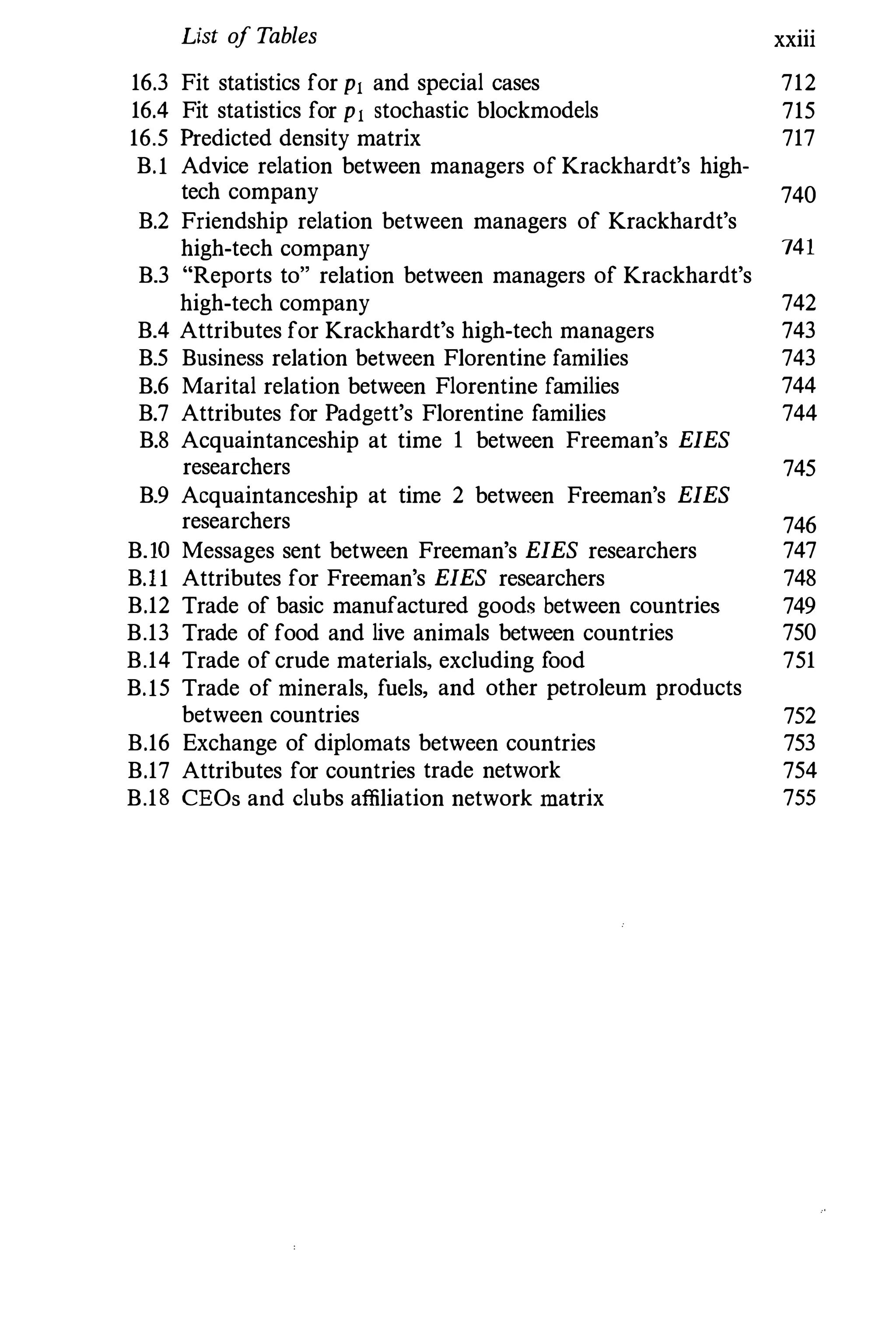
actors might not even be members of a well·defined set of actors. Clearly
in these instances, we are not studying a network with a boundary. We
refer to such studies as special network designs.
In the next paragraphs, we discuss data collection procedures for
cognitive social structure designs, experimental, ego-centered networks,
and small- and reverse small-world techniques.
Cognitive Social Structure. In a standard sociometric question­
naire, one asks respondents about their own ties. A variation of this
design is to ask respondents to give information on their perceptions
of other actors' network ties. Such designs are called cognitive social
structures because they measure perceived relations (Krackhardt 1987a;
Kumbasar, Romney, and Batchelder n.d.).
As an example, Krackhardt and Porter (1985) studied turnover in
several fast food restaurants. They were interested in the employees'
52 Social Network Data
perceptions of friendships among all other employees in the restaurant.
Thus, they had to gather information from each person not only about
their own friendships, but also about their perceptions of the friendships
among all other pairs of employees. They collected network data at two
points in time.
Their procedure is described as follows:
In the first questionnaire, each person in the work group was asked
to record who they perceived to be a friend of whom. While simple
on the surface, this substantial task required that employees consider
all possible pairs of friends in the restaurant. To accomplish this, the
respondent was told to check the names of all those listed whom he
or she thought would be considered a friend by employee # 1 (for
example, "Henry"), Then, the same list was r�peate<..l on the next page,
and the respondent was asked to check all names of those whom he
or she thought would be considered a friend of employee # 2 ("Rita").
This process was repeated a total of N times (for N employees). In
this way, we could assess each person's perception of everyone's friends,
their own as well as their coworkers. (page 250)
Alternatively, one can ask respondents to report subgroups of people
who form relatively tightly knit subgroups within the larger collection of
people (Freeman, Freeman, and Michaelson 1988, 1989).
Data collected using a cognitive social structure design gives consid­
erably more information than the usual sociometric design, since actors
report not only on their own ties, but also on their perceptions of ties
among all pairs of actors.
Experimental. Social network data can be collected using exper­
imental designs. There are (at least) two basic ways to conduct such
experiments. First, one can choose a set of actors and observe their in­
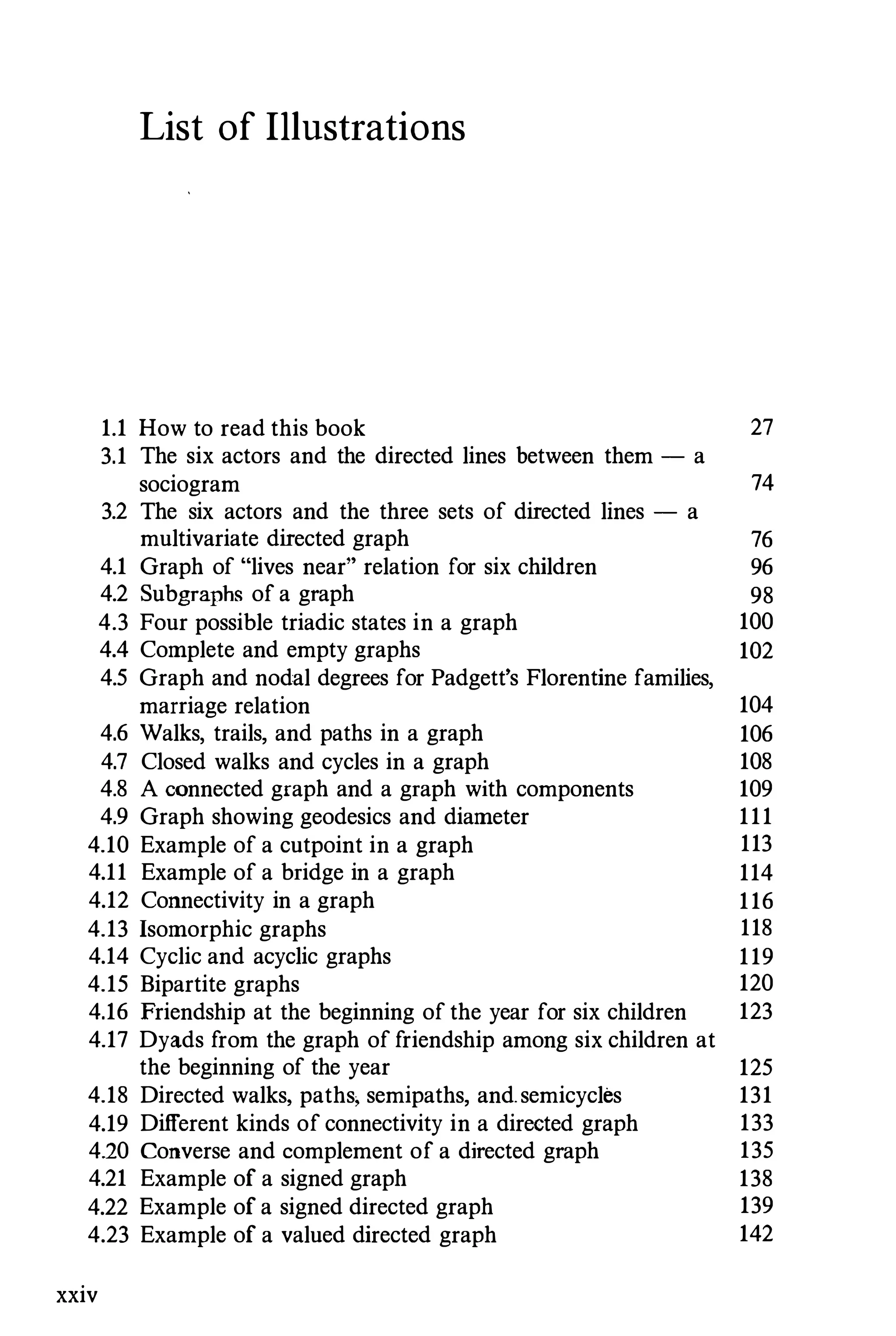
teractions in an experimentally controlled situation. The researcher then
records interactions or communications between pairs of actors. Ties
may be observed between all pairs of actors. Second, one can not only
choose actors but also specify which pairs ofactors are permitted to com­
municate with each other during the experiment. One only records the
frequency or content of communications between those pairs of actors
who are permitted to interact.
Group problem-solving experiments (Bavelas 1950; Leavitt 1949, 1951)
in which actors are assignedto positions within the network defined by the
experimenter and allowed to communicate only with specific others are an
example of the second type of experiment. The experimenter manipulates
both group members and their ties. Power and exchange experiments are
2.4 Network Data, Measurement and Collection 53
also of the second type (Cook, Emerson, Gilmore, and Yamagishi 1983;
Bonacich 1987; Markovsky, Willer, and Patton 1988; and Friedkin and
Cook 1990). The experimenter assigns actors to positions, and allows
certain pairs of actors to negotiate the exchange of reSOurces.
Ego-centered. An ego-centered, or local, network consists of a
focal person or respondent (ego), a set of alters who have ties to ego,
and measurements on the ties from ego to alters and on the ties between
alters. One begins by asking a collection of respondents about their ties
to other people to elicit the set of alters. In 1985 the NORC General
Social Survey (see Burt 1984, 1985) asked a sample of 1531 people
From time to time, most people discuss important matters with other
people. Looking back over the past six months, who are the people
with whom you discussed matters important to you? (page 1 19)
One also asks respondents information about the ties among the people
that the respondent has named. The 1985 General Social Survey COn­
tained a question about the ties among all pairs of people named by
the respondent. If we label two of the people named by a particular
respondent "Alter 1" and "Alter 2," then the question can be worded
Please think about the relations between the people you just mentioned.
Some of them may be total strangers, in the sense that they would
not recognize each other if they bumped into each other on the street.
Others might be especially close, as close to each other as they are to
you. First think about [Alter 1] and [Alter 2]. Are these people total
strangers? (Burt 1985, page 120)
Such measurements give rise to ego-centered networks.
Small World. Special network designs are also used in small
world and reverse small world studies. A small world study is an attempt
to delermine how many actors a respondent is removed from a target
individual based on acquaintanceship. Ofprimary interest is not only how
long these "chains" are, but also the characteristics of the intermediate
actors in the chain. This data collection design was pioneered by Milgram
(Milgram 1967; Travers and Milgram 1969). Korte and Milgram (1970)
describe the typical small world study as follows:
The small world method consists of presenting each of the persons in a
"starting population" with the description of a given "target person" ­
his name, address, occupation, and other selected information. The task
ofa starter is to advance a: booklet toward the target person by sending
54 Social Network Data
the booklet to a personal acquaintance whom he considers more likely
than himself to know the target. Each person in turn advances the
booklet in this manner until the chain reaches the target (page 101)
Often the intermediaries are asked to return a postcard to the researcher
reporting some basic demographic characteristics. The researcher can
then compare characteristics of successful and unsuccessful chains. Korte
and Milgram (1970), Erickson and Kringas (1975), and Shotland (1976)
have also used this design, as discussed by Lin (1989), and by papers in
the volume edited by Kochen (1989).
A reverse small world study focuses on the ties from a specific respon­
dent to a variety of hypothetical targets (Killworth and Bernard 1978;
Cuthbert 1989). Cuthbert (1989) states:
. . . individuals are asked to imagine that they will pass something to
someone who is to eventually reach a target person they do not know.
They are instructed to think of someone they know, who might be a
first link in a chain to the target person. . .. The respondent is given
a list of possible targets who are located geographically and socially
in different parts of the society. In this way the reverse small world
method clearly maps the outgoing network of the people who complete
the questionnaire. (page 212)
White (1970) discusses the possible biases that can arise by using the
small world technique. Many of these biases arise because response rates
are typically much lower with this form ofnetwork data collection. Better
estimation strategies of network properties are discussed by White (1970)
and by Hunter and Shotland (1974).
Diary. Another way to gather social network data is to ask each
respondent to keep a continuous record of the other people with whom
they interact (for example, Gurevich 1961; de Sola Pool and Kochen
1978). Such methods have been used in the study of personal networks
among people. For example, see Cubbitt (1973), Mitchell (1974), and
Higgins, McClean, and Conrath ( 1985).
Social support researchers sometimes ask respondents to keep daily
records of all people with whom they come into contact. In addition
to generating a list of people in every respondent's personal network,
these data sets frequently include information on the type of relation
and characteristics of the alters in each ego-centered network (see Reis,
Wheeler, Kernix, Spiegel, and Nezlek 1985; Pagel, Erdly, and Becker
1987).
2.4 Network Data, Measurement and Collection 55
2.4.3 Longitudinal Data Collection
Occasionally, a researcher is interested in how ties in a network change
over time. In studies of such processes, one measures one or more
relations at fixed intervals of time. Such designs allow one to study how
stable ties are and whether such ties ever reach an equilibrium state.
There are (usually) two research questions to be answered when studying
longitudinal network data. The first is how the process has changed over
time, while the second question asks how well the past, or the history of
the process, can predict the future. Some comments on how to gather
longitudinal social network data can be found in Wasserman (1979).
Longitudinal social network data can be collected using any of the
methods described above (questionnaire, interview, observation, and so
on). There have been some important longitudinal studies, primarily of
sociometric relations, such as friendship. Other researchers have looked
at communications throughout a network over time.
Nordlie (1958) and Newcomb (1961) studied two 1956 University of
Michigan fraternities, each containing seventeen men housed together,
for a period offifteen weeks. All students were incoming transfer students
who were initially unknown to each other. Each person was asked to
rank each of his fellow fraternity members on the basis of positive feeling.
Rankings were recorded each week, except for week 9. These data were
studied in depth by Nordlie (1958), White, Boorman, and Breiger (1976),
Boorman and White (l976), and Wasserman (1980).
Bernard, Killworth, and Sailer (1980, 1982) studied another fraternity
over time, this one existing in the late 1970's in Morgantown, West
Virginia. The fifty-eight fraternity members had been living together at
least three months. Interactions among members within the fraternity
were recorded by an outside observer every fifteen minutes, twenty-one
hours per day, for five days. This observation process was conducted three
times during the year. The observer noted every group in conversation,
yielding a very rich set of longitudinal interaction ties. In addition, the
researchers asked the fraternity members both about their "friendships"
within the fraternity and about their recollections of their interactions
with other fraternity members at the end of each of the three observation
periods. To measure the interaction relation, the students were asked to
give a rating of their interactions with each of the other actors on an
ordinal scale of 1 (no communication) to 5 (great deal ofcommunication).
Thus, three longitudinal relations were studied: interaction (measured
56 Social Network Data
almost continuously for three different five-day periods), friendship, and
recalled communication (measured at three points in time).
Another classic example is Freeman's EIES data, which consist of
measurements of computer mail interactions, over the course of an
eighteen month period, among a set of quantitative researchers studying
social networks. These data arc described at the end of this chapter.
Yet another example comes from Katz and Proctor's (1959) study of ties
in an eighth-grade classroom of twenty-five boys and girls. These data
consist of friendship choices made four times during the school year. The
data were gathered by Taba (1955), who focused on the differences and
similarities between boy-boy and girl-girl choices, and "mixed gender"
ties.
2.4.4 Measurement Validity, Reliability, Accuracy, Error
As we noted in Chapter 1, social network research is concerned with
studying patterns of social structure. As Freeman and Romney (1987)
note, "social structure refers to a relatively prolonged and stable pattern
of interpersonal relations" (1987, pages 330-331). In their discussion of
measurement error in sociometry, Holland and Leinhardt (1973) refer to
this pattern as the true structure, in contrast to the observed structure
contained in the measured network data, which might contain error.
Important concerns in social network measurement are the validity,
reliability, and measurement error in these data. In addition, since
social network data are often collected by having people report on
their own interactions, the accuracy of these self-report data is also a
concern. Surprisingly little work has been done on the issues of validity,
reliability, and measurement error in social network data. A recent paper
by Marsden (1990b) reviews this work; we summarize this and other
research briefly here.
"Accuracy". Often sociometric data are collected by having peo­
ple report on their interactions with other people. For example, a
researcher might ask each actor to report "With whom did you talk
last week?", or "What other people were at the party with you last
Saturday?" In either case, the respondent is asked to recall his or her
interactions. An important issue is the relationship between information
collected using verbal reports and information collected by observing the
peoples' interactions.
2.4 Network Data, Measurement and Collection 57
Considerable research has been done on the question of iriformant
accuracy in social network data. Much of this research was conducted by
Bernard, Killworth, and Sailer using very clever data collection designs
in which they observed interactions among people in several different
communities (for example, a fraternity, a research office, and ham radio
operators) and also asked the same people to report on their interactions
(Bernard and Killworth 1977, 1979; Killworth and Bernard 1976, 1979;
Bernard, Killworth, and Sailer 1980, 1982; Bernard, Killwor!h, Kronen­
feld, and Sailer 1985). They concluded that about half of what people
report about their own interactions is incorrect in one way or another.
Thus, people are not very good at reporting on their interactions in
particular situations.
However, recent studies by Freeman, Romney, and colleagues (Rom­
ney and Faust 1982; Romney and Weller 1984; Freeman and Romney
1987; Freeman, Romney, and Freeman 1987; Freeman, Freeman, and
Michaelson 1988) and by Hammer (1980, 1985) argue that particular
interactions are not of primary concern to social network researchers.
Rather, as we noted above, the "true" structure of the network, relatively
stable patterns of interaction, are of most interest. Thus it is these long­
term patterns the researcher should be studying and estimating, not the
particular interactions of individuals. Freeman, Romney, and Freeman
(1987) argue !hat verbal reports (recall of interactions) should be under­
stood using principles of memory and cognition. They found that what
people report about their interactions is in fact related to the long-range
social structure, rather than to particular instances.
Another issue related to the accuracy of network data occurs when the
actors in the network are organizations (for example corporations) but
information on ties is collected from individuals as representatives of the
organization. For example, Galaskiewicz (1985) measured donations from
corporations to non-profit agencies by interviewing the officer in charge
of corporate giving. One must be able to assume that the individual who
is interviewed in fact has knowledge of the information being sought.
Validity. A measure of a concept is valid to the extent that it
actually measures what it is intended to measure. Often, a researcher
assumes that the measurements of a concept are indeed valid. For
example, one might assume that asking people "Which people in this
group 'are your friends?" has face validity as a measure of friendship, in
the sense that the answer to the question gives a set of actors who are
related to the respondent through friendship ties.
58 Social Network Data
However, the validity of a measure of a concept is seldom tested in a
rigorous way, A more formal notion of validity, construct validity, arises
when measures of concepts behave as expected in theoretical predictions.
Thus, the construct validity of social network measures can be studied
by examining how these measures behave in a range of theoretical
propositions (Monton. Blake, and Fruchter 1955b; Burt, Marsden, and
Rossi 1985).
Very little research on the construct validity of measures of network
concepts has been conducted. In one study of this important idea,
Mouton, Blake, and Fruchter (1955b) reviewed dozens of sociometric
studies and found that sociometric measnres, such as number of choices
received by an actor, were related to a number of actor characteristics,
such as leadership and effectiveness, thus demonstrating the construct
validity of those sociometric measures.
Reliability. A measure of a variable or concept is reliable if
repeated measurements give the same estimates of the variable. In a
standard psychometric test-theoretic framework (see Lord and Novick
1968; Messick 1989), the reliability of a measure can be assessed by com­
paring measurements taken at two points in time (test-retest reliability),
or by comparing measurements based on subsets of test items (split­
halves or alternative forms). For the test-retest assessment of reliability
to be appropriate, one must assume that the "true" value of a variable
has not changed over time. This assumption is likely to be inappropriate
for social network properties, since social phenomena can not be assumed
to remain in stasis over any bnt the shortest spans of time. Assessing
reliability of social network measurements using the test-retest approach
is therefore problematic. Three approaches that have been used to assess
the reliability of social network data are: test-retest comparison, compar­
ison of alternative question formats, and the reciprocity of sociometric
choices (Conrath, Higgins, and McClean 1983; Hammer 1985; Laumann
1969; Tracy, Catalano, Whittaker, and Fine 1990).
Reliability of sociometric data can also be assessed at different levels.
One can study the reliability of the "choices" made by individual actors,
or one can study the reliability of measures aggregated over a number of
individual responses (for example, the popularity of an actor measured
as the total number of choices it received) (Mouton, Blake, and Fruchter
1955a; Burt, Marsden, and Rossi 1985).
Although it is difficult to draw general conclusions from the research
on the reliability of social network data collected from interviews or
2.5 Data Sets Found in These Pages 59
questionnaires, several findings are noteworthy. Sociometric questions
using ratings or full rank orders are more reliable (have higher test-restest
reliability) than fixed choice designs in which just a few responses are
allowed (Mouton, Blake, and Fruchter 1955a). Responses to sociometric
questions about more intense or intimate relations have higher rates of
reciprocation than sociometric questions about less intense or intimate
relations (see Marsden 1990b; Hammer 1985). Lastly, the reliability of
aggregate measures (such as popularity) is higher than the reliability of
"choices" made by individual actors (Burt, Marsden, and Rossi 1985).
Measurement Error. Measurement error occurs when there is
a discrepancy between the "true" score or value of a concept and the
observed (measured) value of that concept. It is common to assume that
the observations or measurements of a concept are an additive combina­
tion of the "true" score plus error (or noise). This error, the difference
between the true and observed values, is referred to as measurement error.
Holland and Leinhardt (1973) present a thorough discussion of mea­
surement error and its implications in social network research. As they
note, in social network research the measurements are the collection
of ties among actors in, the network, represented in the sociomatrix or
sociogram. These measurements may differ from the "true" structure of
the network. Since there are several levels at which we can study social
networks (for example, one can look at properties of actors, pairs of
actors, subsets of actors, or the network as a whole), it is important to
understand the implications of measurement error at each of these levels.
Of particular importance in the discussion presented by Holland and
Leinhardt is the error that arises in fixed choice data collection designs.
Recall that in a fixed choice design, the respondent is instructed to
nominate or name some fixed number of others for each relation. For
example, each person may be asked to "List your three best friends."
This design introduces error since it is quite unlikely that all people have
exactly three best friends. The restriction of the nomination process also
introduces error into the measurement of other network properties, such
as properties of triads (triples of actors and their ties) and of subgroups.
2.5 Data Sets Found in These Pages
We now turn our attention to the network data sets that we focus on
throughout this book. Each is described in detail, with attention given
to the issues mentioned earlier in the chapter. All of these data sets,
60 Social Network Data
including measurements on all relations and actor attributes (if included)
can be found in Appendix B. As the reader will see, these data are quite
diverse, coming from a variety of disciplines and theoretical concerns.
There are five primary data sets we discuss below.
2.5.1 Krackhardt's High-tech Managers
This is a one-mode network, with three relations measured on a set of
people. These data were gathered by Krackhardt (1987a) in a small man­
ufacturing organization on the west coast of the U.S. This organization
had been in existence for ten years and produced high-tech machinery for
other companies. The firm employed approximately one hundred people,
and had twenty-one managers. These twenty-one managers are the set
of actors for this data set. Throughout the book, we will refer to this
example as "Krackhardt's high-tech managers." Krackhardt's interest in
these data focused on the managers' perceptions of the entire network of
informal advice and friendship relations. Specifically, he was interested
in the perceptions held by the managers of the structure of the entire
network. N; we note later, he gathered much more extensive data than
we will use. Here, we are interested only in the reports made by each
manager of his or her own advice seeking and friendships.
Each manager was given a questionnaire and asked two questions:
"Who would [you] go to for advice at work?" and "Who are your
friends?" Each manager was given a roster of the names of the other
managers, and asked (in a free choice setting) to check the other managers
to whom they would go for advice at work, and with whom they were
friends. Krackhardt also gathered a third relation based on the official
organizational chart. He recorded "who reports to whom" for all twenty­
one managers.
Thus, this is a multirelational data set, with three relations : "advice,"
"friendship," and "reports to." All three are dichotomous and directional.
The first two were gathered from questionnaires, and the third, from
organizational records. These relations were measured for a single point
in time. The friendship relation clearly is an individual evaluation, while
the advice relation is a verbal report of an interaction between actors.
The third relation is a measurement of the formal bureaucratic structure
within the organization. So, this data set has three very different types
of relations.
The network is one-mode, since we have just a single set of twenty-one
actors. The actors are people. This data set also includes four actor
2.5 Data Sets Found in These Pages 61
attributes : age; length of time employed by the organization (tenure);
level in the corporate hierarchy; and the department. The first two are
measured in years. There are four departments in the firm. All but the
president of the firm have a department attribute coded as an integer
from 1 to 4. The level attribute is measured on an integer scale from 1
to 3 : 1 = CEO, 2 = vice president, and 3 = manager.
Of primary interest to Krackhardt were the perceptions held by each
actor of the friendships and advice seeking within the firm. Each actor
was asked to evaluate all the ties between all actors, not just the ties
involving the respondent. In this way, Krackhardt was able to study
perceptions of network structure. For example, how were an actor's
actual reported friendships perceived by all the other acto",? Krackhardt
(1987a) categorized actors by their importance (as measured by centrality
indices) and found that more important actors had better perceptions
than those less important.
2.5.2 Padgett's Florentine Familie:,'
This is a one-mode network with two relations measured among a set
of families. These multirelational network data, compiled by Padgett,
consist of the marriage and business ties among 16 families in 15th
century Florence, Italy. These data were compiled from the history of
this period given by Kent (1978). The 16 families were chosen for analysis
from a much larger collection of 116 leading Florentine families because
of their historical prominence. Padgett (1987), Padgett and Ansell (1989,
1993), and Breiger and Pattison (1986) have extensively analyzed these
data. Throughout, we will refer to this example as "Padgett's Florentine
families."
The actors in this network are families. As noted by Breiger and
Pattison, the family was an important et::onomic and political unit, so
the history of 15th century Florence can be well understood by focusing
on families, rather than individual people. In the early 1430's, a political
battle was waged in Florence for control of the government, primarily
between the Medicis and the Strozzis, two of the families included in this
data set. An excellent account of this history can be found in Padgett
(1987). We note that Padgett and Ansell (1989) studied seventy-one
families, and were interested in how the Medici family rose to dominate
Florence between 1427 and 1434. Of primary interest to them was the
association between the two relations, marriage and business.
62 Social Network Data
The two measured relations are marriage and business. Both are
nondirectional and dichotomous, and are transactional, since the business
relation as well as the marital ties were used to solidify political and
economic alliances. A marital tie exists between a pair of families if
a member of one family marries a member of the other. A business
tie exists if, for example, a member of one family grants credits, makes
a loan, or has a joint business partnership with a member of another
family (Breiger and Pattison 1986).
For these data, Padgett was not able to determine how families married
each other or how families did business with each other. This nondirec­
tionality is proper for marital ties, but perhaps not for business dealings.
A variety ofauthors (including Breiger and Pattison 1986) have remarked
that the nondirectionality of the business relation is unfortunate, since
loans and credits are clearly directed from one family to another. More
recent research by Padgett and Ansell (1993) contains an updated coding
of the marriage relation that records both the family for the bride and
the family for the groom, so that a directional marital relation can be
studied. Both relations reflect activities occurring during this time period,
but are not longitudinal.
The actors are families, 16 in number. There are three actor attributes:
net wealth in 1427 (as taken from government records) ; number ofpriors
(seats on the city council) from 1282-1344; and number of business or
marriage ties in the total network (consisting of all 116 families).
2.5.3 Freeman's EIES Network
This is a one-mode network with two relations measured on a set of
people. These data come from a computer conference among researchers
working in the emerging scientific specialty of social network research,
organized by Freeman, and sponsored by the National Science Foun­
dation. These data were collccted as part of a study of thc impact of
the Electronic Information Exchange System (EIES) housed at the New
Jersey Institute of Technology. Fifty researchers interested in social net­
work research participated. We focus here on the thirty-two people who
completed the study. These researchers included sociologists, anthro­
pologists, and statisticians/mathematicians. As part of the conference,
a computer network was set up and participants were given computer
terminals and access to a network for sending electronic mail messages
to other participants. We note that this study was done prior to the
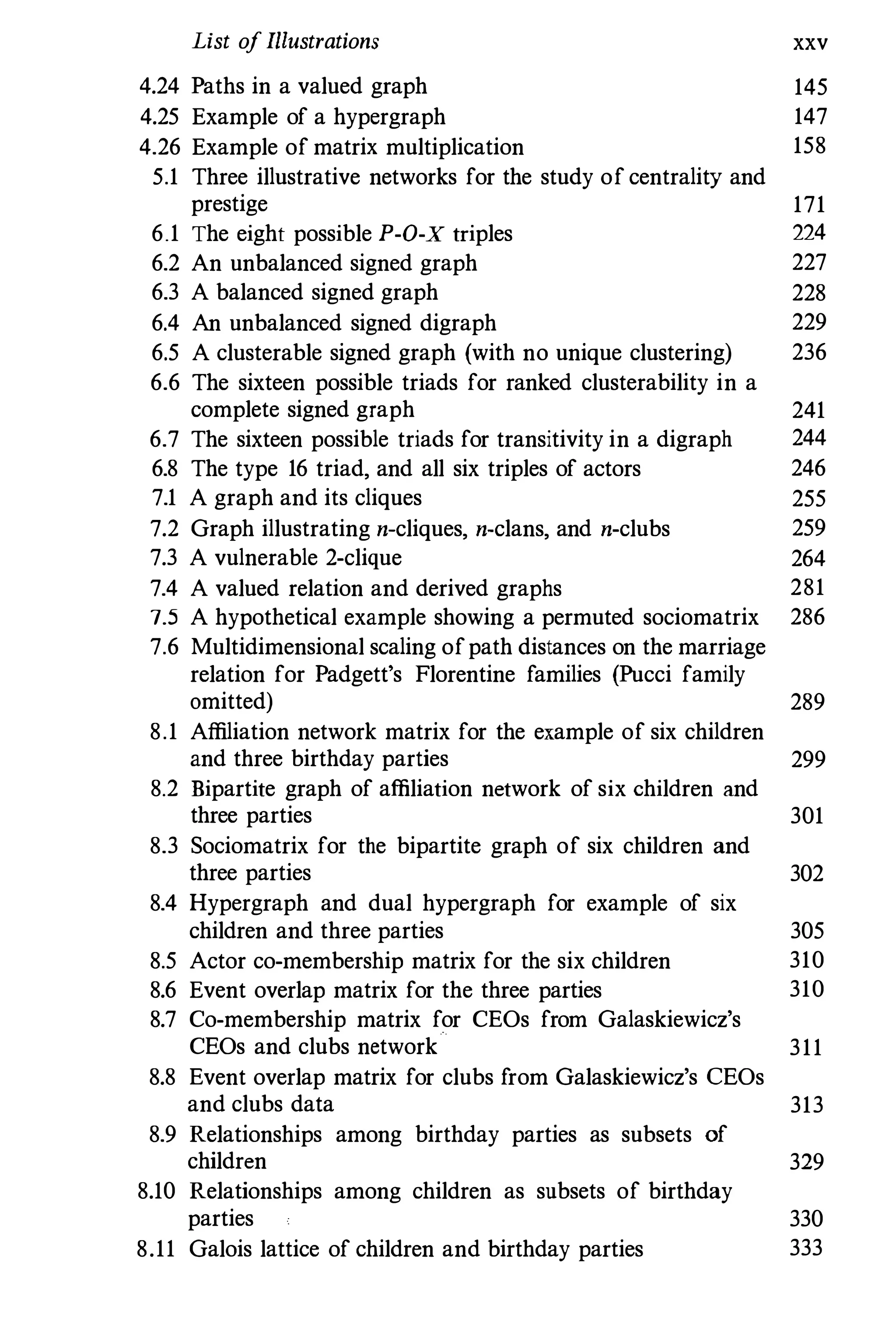
widespread use of BITNET, INTERNET, and other popular computer
2.5 Data Sets Found in These Pages 63
networks that are widely available to academics today; consequently, this
study involved a novel way for researchers to communicate. For more
details of this study, see S. Freeman and L. Freeman (1979), L. Freeman
and S. Freeman (1980), and Freeman (1986). A more detailed description
of the design of this study can be found in Bernard, Killworth, and Sailer
(1982). Here, we will refer to this example as "Freeman's EIES network."
Of particular interest are the network data arising from this study. Two
relations, messages sent and acquaintanceships, were recorded. As part
of this project, the computer system recorded all message transactions,
specifically the origin and destination of the message, the day and time,
and the number of lines in the message. Records were kept for several
months. We therefore have a record of the number ofmessages sent from
each participant to every other participant. We restrict our attention to
the total number of messages sent from one actor to another; however,
this message-sending relation can be defined for any time interval, for
example, the number of messages sent in a given month. A second
relation is acquaintanceship, and was gathered by a questionnaire. At the
beginning and at the end of the project, participants were asked to fill out
a questionnaire that included, among other things, a network question.
Each participant was asked to indicate, for every other participant,
whether she/he: (1) did not know the other, (2) had heard ofthe other but
had not met him/her, (3) had met the other, (4) was a friend of the other,
or (5) was a close personal friend of the other. This acquaintanceship
relation is longitudinal, measured at two points in time: at the beginning
ofthe study (January 1978), and at the end (September 1978) (S. Freeman
and L. Freeman 1979).
There are two attribute variables in this data set: Primary disciplinary
affiliation of the person; and Number of citations of the researcher's
work in the Social Science Citation Index for the year 1978 (when the
research started). The disciplinary affiliation variable has four categories :
(1) sociology, (2) anthropology, (3) mathematics or statistics, and (4)
other. The citation variable is coded as the number of citations.
These data are a part of a more comprehensive data set gathered
by Bernard (who, along with Freeman, supplied us with these data)
to study the accuracy of informants' reports of communications (see
Bernard, Killworth, and Sailer 1982). Freeman (1986) studied the impact
of this newly formed computer network on the acquaintanceship� and
friendships among the network researchers. Wasserman and Faust (1989)
used these data to demonstrate the application of correspondence and
canonical analysis to social network data.
64 Social Network Data
2.5.4 Countries Trade Data
This is a one-mode network with five relations measured on countries.
These data were gathered by us for use in this book. The actors are
countries, selected from a list of sixty-three countries given in Smith
and White (1988). We chose countries representing different categories
from across several developmental classifications: Snyder and Kick's
(1979) core/periphery status, Nemeth and Smith's (1985) alternative
world system classification and level of industrialization, and a historical
economic base from Lenski (as reported in Breedlove and Nolan 1988).
We also chose countries both to span the globe and to represent politically
and economically interesting characteristics. Only countries for which
data were reported in 1984 commodity trade statistics were eligible for
inclusion. We also attempted to reduce the number of shared borders
between countries; however, some politically interesting countries are
included even though they share borders (Israel and Syria, for example).
Because of data availability, less-developed nations (African nations in
particular) are probably under-represented in this set.
The final twenty-four countries represented as actors in this network
are a geographically, economically, and politically diverse set, chosen
to represent a range of interesting features and to span the categories
of existing world system/development typologies. We will refer to these
data as the countries trade network. Because of the selection mechanism,
we will assume that this set of actors is representative of all possible
countries.
Five relations were measured. Four of them are economic and one is
political. The relations are:
• Imports of food and live animals
• Imports of crude materials, excluding fuel
• Imports of mineral fuels
• Imports of basic manufactured goods
• Diplomatic exchange
The first four relations are taken from the United Nations Commodity
Trade Statistics (1984). We chose these four types of commodities (with
single digit section codes 0, 2, 3, and 6 from the commodity trade
statistics) since these commodities were studied originally by Breiger
(1981a). The last relation comes from The Europa Year Book (Europa
Publications 1984), which lists for each country those countries that have
embassies or high commissions in the host country.
2.5 Data Sets Found in These Pages 65
All five relations are dichotomous and directional. The four economic
relations were reported on a continuous US$ scale. The reported values
indicate the amount of goods (of the specified type) in 100,000 US$
imported by one country from the other (the UN does not list trade
amounts under 100,000 US$). In order to standardize the imports to
control for the vastly different economy sizes across countries, we first
standardized each value by dividing by the country's total imports on
that commodity. If the realized proportion was less than 0.01 %, we
coded the tie as absent. Otherwise, the tie was coded as present. This
standardization actually had very little impact. Most of the ties that were
changed from "trade present" to "trade absent" were large countries
(US, Japan, UK) importing small amounts from very small countries
(Madagascar, Liberia, Ethiopia).
The diplomatic relation records a tie as present if one country has an
embassy or a high commission in another country. These data are taken
from the 1984 Europa Year Book (Europa Publications 1984).
The data set includes four attribute variables reflecting the economic
and social characteristics ofthe countries. The first two attribute variables
measure annual rates of change between 1970 and 1981. They are:
Annual population growth rate between 1970 and 1981, and Annual
growth rate in GNP per capita between 1970 and 1981. The second two
attribute variables measure rates of education and energy consumption.
These variables are: Secondary school enrollment ratio in 1980, and
Energy consumption per capita in 1980 (measured in kilo coal equivalent).
Researchers have argued that these variables are related either to level
of national development (industrialization) or to world system status.
Measurements on these four variables were taken from The World Bank
(1983).
Numerous social scientists have used network methods and data to
study the world political and economic system (Snyder and Kick 1979;
Nemeth and Smith 1985; Breiger 1981c). These researchers are primarily
interested in whether location in a network "system" affects the rates of
industrialization and development.
2.5.5 Galaskiewicz's CEOs and Clubs Network
This data set is a two-mode, affiliation network. The .first mode consists
of twenty-six chief executive officers (and spouses) of the major corpora­
tions, banks, and insurance companies headquartered in the Minneapo­
lislSt. Paul metropolitan area. These data were gathered by Galaskiewicz
66 Social Network Data
through interviews with the CEOs and records of the clubs and boards.
Thus, the first mode is a set of corporate CEOs as actors. The sec­
ond mode is a collection of fifteen clubs, cultural boards, and corporate
boards of directors to which the CEOs belong. There are two coun­
try clubs (Woodhill Country Club and Somerset Country Club), three
metroplitan clubs (Minnesota Club, Minneapolis Club, and the Womens
Club), four prestigious cultural organizations (such as Guthrie Theater,
Minnesota Orchestra Society, Walker Art Center, SI. Paul Chamber Or­
chestra, Minnesota Public Radio), and the six corporate boards of the
FORTUNE 500 manufacturing firms and FORTUNE 50 banks head­
quartered in the area. These data record which CEO belongs to each of
the clubs andboards. These memberships are for 1978-1981 (as discussed
by Galaskiewicz 1985). We will refer to these data as Galaskiewicz's CEOs
and clubs.
All data are dichotomous, indicating presence or absence of a mem­
bership. The first mode is a set of people, and the second, a set of
organizations. The data are affiliational, and represent memberships.
There are a number of attributes that are measured for both modes. For
the first mode, we can categorize the actors by the nature of the corpo­
rations they head. For the second, we can categorize the organizations
by their nature (clubs or corporate boards).
2.5_6 Other Data
In addition, we analyze a hypothetical data set throughout the book.
This data set is used mostly to illustrate calculations, and consists of
six second-grade children. It has measurements on four relations, three
measured for the first mode (a set of six children) and one for actors in
the first mode choosing actors in the second mode (a set of four teachers).
One ofthe relations is longitudinal - friendship at the beginning and end
of the school year. In addition, we have a single affiliation relation (party
attendance). There are also a number of attributes that are recorded for
both children and teachers, which will be introduced as needed.
Part II
Mathematical Representations of
Social Networks
3
Notation for Social Network Data
Social network data consist of measurements on a variety of relations
for one or more sets of actors. In a network data set we may also have
recorded information on attributes of the actors. We will need notation
for the set of actors, the relations themselves, and the actor attributes so
that we can refer to important network concepts in a unified manner.
In this chapter, we introduce notation and illustrate with examples.
We start by defining notation for a single, dichotomous relation. We then
move to more complicated network data sets involving more than one set
of actors and/or more than one relation. We will need a notational system
flexible enough to handle the wide range of network data sets that are
encountered in practice. We note that the only type of structural variable
discussed in this chapter is relational. Chapter 8 presents notation and
methodology for affiliational networks.
For the reader who already is familiar with social networks and the
ways in which social network data can be denoted, or the reader who
is only interested in specific techniques, we recommend a quick reading
of the material in this chapter. Specifically, such readers can glance at
Section 2 and the examples used in this chapter (perhaps skipping the
material on multiple relations), and return to this chapter as needed.
There are many ways to describe social network data mathematically.
We will introduce three different notational schemes. These schemes can
each be adapted to represent a wide range of network data. However, for
some forms of data and some types of network methods, one notation
scheme may be preferred to the others, because of its appropriateness,
clarity, or efficiency. The notations are:
• Graph theoretic
• Sociometric
69
70 Notation for Social Network Data
• Algebraic
Each scheme will be described and illustrated in detail. We will show how
these schemes overlap, and discuss when a specific scheme is more useful
than the others. Graph theoretic notation is most useful for centrality and
prestige methods, cohesive subgroup ideas, as well as dyadic and triadic
methods. Sociometric notation is often used for the study of structural
equivalence and blockmodels. Algebraic notation is most appropriate for
role and positional analyses and relational algebras. We should note that
there are other ways to denote social network data, some of which are
used to study specific statistical models. Such schemes will be mentioned,
when needed, in later chapters.
The graph theoretic notation scheme can be viewed as an elementary
way to represent actors and relations. It is the basis of the many concepts
of graph theory used since the late 1940's to study social networks.
The notation provides a straightforward way to refer to actors and
relations, and is completely consistent with the notation from the other
three schemes. Mathematicians and statisticians such as Bock, Harary,
Katz, and Luce were among the first to view networks as directed and
undirected graphs (see Forsyth and Katz 1946; Katz 1947; Luce and
Perry 1949; Bock and Husain 1950, 1952; Harary and Norman 1953).
Graph theory texts such as Flament (1963) and Harary (1969) describe
social network applications. We should also direct the reader to other
texts on graph theory and social networks, such as Harary, Norman,
and Cartwright (1965), and Hage and Harary (1983), that present graph
theoretic notation for social network data. Mathematical sociology texts,
such as Coleman (1964), Fararo (1973), and Leik and Meeker (1975),
contain elementary discussions of the use of graph theory in social
network analysis.
The second notation scheme, sociometric notatiol1, is by far the most
common in the social network literature. One presents the data for each
relation in a two-way matrix, termed a sociomatrix, where the rows and
columns refer to the actors making up the pairs. Sociomatrices began
to be used more than fifty years ago after their introduction by Moreno
(1934) in his pioneering research in sociometry (see also Moreno and
Jennings 1938).
Most major computer software packages for social network data an­
alyze network information presented in sociomatrices. Further, many
methods are defined for sociomatrices. This notational scheme is prob­
ably the most useful for readers interested in the methods discussed
3.1 Graph Theoretic Notation 71
in Parts III and IV of the book. Sociomatrices are adjacency matrices
for graphs, and consequently, this second notational scheme is directly
related to the first.
The third notational scheme, algebraic notation, is used to study
multiple relations. This notation is useful for studying network role
structures and relational algebras. Such analyses use algebraic techniques
to compare and contrast measured relations, and derived compound
relations. A compound relation is the composition or combination of
two or more relations. For example, if we have measured two relations,
"is a friend of" and "is an enemy of," for a set of people, then we
might be interested in the composition of these two relations : "friends'
enemies." The focus of such algebraic techniques is on the associations
among the relations measured on pairs of actors,. across the entire set of
actors. This notation is designed for one-mode networks, and was first
used by White (1963) and Boyd (1969).
We now turn to each of these notations, show how they are related,
discuss when each is useful, and illustrate each with examples.
3,1 Graph Theoretic Notation
A network can be viewed in several ways. One of the most useful views
is as a graph, consisting of nodes joined by lines. Chapter 4 discusses
graph theory at length. Here, we introduce some simple graph theoretic
notation, and show how this notation can be used to label the actors and
relations in a network data set.
Suppose we have a set of actors. We will refer to this set as %.
The set % contains g actors in number, which we will denote by %
= {n" n" . . . ,ng}. The symbol % is commonly used to stand for the
set, sinoe the graph theory literature frequently refers to this set as a
collection of !lodes of a graph. For example, consider a collection of
g = 6 second-grade children: Allison, Drew, Eliot, Keith, Ross, and
Sarah. We have % = {Allison, Drew, Eliot, Keith, Ross, Sarah}, a
collection of six actors, so that we can refer to the children by their
symbols: n, = Allison, n, = Drew, n3 = Eliot, n4 = Keith, ns = Ross,
and n6 = Sarah.
3,1,1 A Single Relation
We now assume that we have a single relation for the set of actors %.
That is, we record whether each actor in % relates to every other actor
72 Notationfor Social Network Data
on this relation. To start, we will let the relation be dichotomous and
directional. Thus, n, either relates to nj or does not. For now, we do not
consider the strength of this interaction or how frequently n, interacts
with nj-
Consider an ordered pair of actors, n, and nj. Either the first actor in
the ordered pair relates to the second or it does not. Since the relation is
directional, the pair of actors n, and nj is distinct from the pair nj and n,
(that is, order matters). If a tie is present, then we say that the ordered
pair is an element of a special collection of pairs, which we will refer to
as !t? If an ordered pair is in !t?, then the first actor in the pair relates
to the second on the relation under consideration.
Note that there can be as many as g(g - 1) elements (the total number
of ordered pairs in !t?), and as few as O.
If the ordered pair under consideration is < n" nj >, and if there is
a tie present, we will write n, --+ nJ. The elements, or ordered pairs, of
relating actors in !t? will be denoted by the symbol !. Let us assume that
there are L entries in !t?, so that !t? = {II,I" ... ,ld. The elements in !t?
can be represented graphically by drawing a line from the first actor in
the element to the second. It is customary to refer to such a graph as a
directed graph, since the lines have a direction. Directed lines are referred
to as arcs. We use the symbol !f to refer to the set of directed Lines and
the symbol I to refer to the individual directed lines in the set. We will
frequently refer to such ordered pairs of relating actors as directed lines
or arc.�.
Since a graph consists of a set·,of nod�s ..A', and a set of lines .se, it
can be described mathematically by the two sets, (.#", !f). We will use
the symbol <"fj to denote a graph. It .is important fa note that for the ·
graph theoretic notation.s.cherne, these.two sets (a set of actors, and a set
of ordered pairs of actors, or arcs) suffice for mathematica) descriptions
of the crncial components in a network on which a single. dichotomous
relation is meaSl.lXed
On some relations, an individual actor does not usually relate to itself.
When studying such relations, one does not consider self-choices.
There are relations that are nondirectional, that is, we cannot distin­
guish between the line from n, to nj and the line from nj to n,. For
example, we may consider a set of actors, and record whether they "live
near each other." Clearly, this is a nondirectional relation - if n, lives
near nj' then nj lives near nj. There is only one measurement to be
made for each pair, rather than two as with a. directional relation. The
two ordered pairs have identical relational interactions. The set !f now
3.1 Graph Theoretic Notation 73
contains at most gig- 1)/2 pairs. The order ofthe pair of actors in these
relating pairs no longer matters, since both actors relate to each other in
the same way.
Return to our example, and suppose that the single, dichotomous
directional relation is "friendship," so that we consider wbetber each
child views every other cbild as a friend. Suppose further that eight
of the possible tbirty ordered pairs are friendships (tbat is, eight of tbe
tbirty possible arcs are present) and tbat the other twenty-two are not
friendships (or that there are twenty-two arcs absent). Let these L = 8
pairs be <Allison, Drew>, <Allison, Ross>, <Drew, Sarah>, <Drew,
Eliot>, <Eliot, Drew>, <Keitb, Ross>, <Ross, Sarah>, and <Sarab,
Drew>. Tbus, for tbe elements of :t', Z, = <Allison, Drew>, 12 =
<Allison, Ross>, . . . , and 18 = <Sarah, Drew>. The data tell us tbat
Allison views Drew as a friend, Allison also views Ross as a friend, Drew
states tbat Sarah is bis friend, and so fortb. It is also interesting to note
that tbis friendship is not reciprocal; that is, if n, states that nj is his
friend (or n, -+ nj), it is possible tbat tbis sentiment is not returned -
nj may not "cboose" n, as a friend (or nj -I-> n,).
A graph can be presented as a diagram in which nodes are represented
as points in a two-dimensional space and arcs are represented by directed
arrows between points. Thns, tbese six cbildren can be represented as
points in a two-dimensional space. It is important to note tbat the actual
location of points in tbis two-dimensional space is irrelevant. We can take
tbese points, and draw in the eigbt arcs representing these eight ordered
pairs of children who are friends. This directed graph or sociogram is
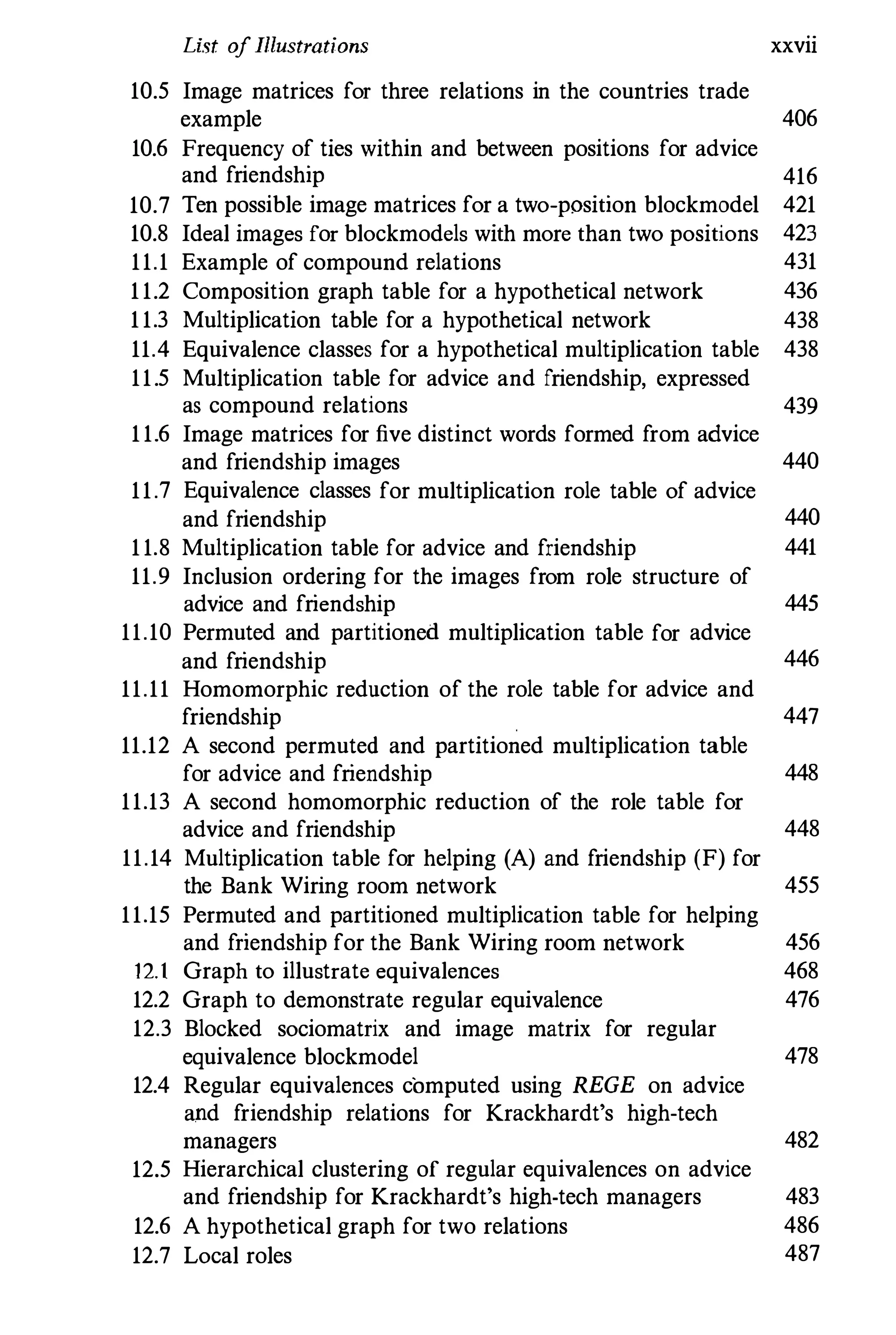
.
shown in Fignre 3.1. .
3.1.2 OMultiple Relations
We may have more than one relation m a social network data set.
O'raph theoretic notation can be generalized to multirelatiorial networks,
which could include both directional and nondirectional relations. For
example, we may study whether tbe corporations in a metropolitan area
do business with eacb other - does n, sell to nj, for example - and
whether fhey interlock tbrough tbeir boards ofdirectors - does an officer
of corporation n, sit on the board of directors of corporation nj? Given
the notation presented for the case of a single dichotomous relation, it is
easy to generalize it to multiple relations.
Suppose that we are interested in more than one relation defined
on pmrs of actors taken from %. Let R be tbe number of relations.
74 Notation for Social Network Data
Allison Drew
.--------------------+. •
•
Eliot
Keith
----- .
. ---
Ross
Fig. 3.1. The six actors and the directed lines between them - a
sociogram
Each of these relations can be represented as a graph or directed graph;
hence, each has associated with it a set of lines or arcs, specifying
which (directed) lines are present in the (directed) graph for the relation
(or, which (ordered) pairs are "relating"). Thus, each relation has a
corresponding set of arcs, 2" which contains L, ordered pairs of actors
as elements. Here, the subscript r ranges from 1 to R, the total number
of relations.
Each of these R sets defines a directed graph on the nodes in ff. These
directed graphs can be viewed in one or more figures. So, each relation
is defined on the same set of nodes, but each has a different set of arcs.
Thus, we can quantify the rth relation by (ff, 2,), for r = 1, 2, . . . , R.
For example, return to our second-graders, and now consider R = 3
relations : 1) who chooses whom as a friend, measured at the beginning
of the school year; 2) who chooses whom as a friend, measured at the
end of the school year; and 3) who lives near whom. The first two
relations are directional, while the last is nondirectional. Suppose that
L] = 8 ordered pairs of actors, L2 = 1 1, and LJ = 12. Below, we list
these three sets.
3.1 Graph Theoretic Notation 75
Relation 1 Relation 2 Relation 3
Friendship at Friendship at Lives
Beginning End Near
<Allison, Drew> <Allison, Drew> (Allison, Ross)
<Allison, Ross> <Allison, Ross> (Allison, Sarah)
<Drew, Sarah> <Drew, Sarah> (Drew, Eliot)
<Drew, Eliot> <Drew, Eliot> (Keith, Ross)
<Eliot, Drew> <Drew, Ross> (Keith, Sarah)
<Keith, Ross> <Eliot, Ross> (Ross, Sarah)
<Ross, Sarah> <Keith, Drew>
<Sarah, Drew> <Keith, Ross>
<Ross, Keith>
<Ross, Sarah>
<Sarah, Drew>
For a non.directional relation, such as "lives near," measurements are
made on unordered rather than ordered pairs. Clearly, when one actor
relates to a second, the second relates to the first; therefore, since Allison
lives near Ross, Ross lives near Allison. When listing the pairs of relating
actors (or arcs) for a nondirectional relation, each pair can be listed no
more than once. We use (., .) to denote pairs of actors for whom a tie is
present on a nondirectional relation, and use < ., . > to denote ties on
a directional relation.
Examining such lists can be difficult. An alternative way to present
the three sets £'" £'2, and £'3 is graphically. We can place the arcs for
directed graphs or lines for undirected graphs on three figures (one for
each relation), or on a single figure containing points representing the six
actors and arcs or lines for all relations, simultaneously. We use different
types of lines in Figure 3.2 for the different relations: solid, for relation 1
(friend at beginning); dashed, for relation 2 (friend at end); and dotted,
for relation 3 (lives near). Since friendship is a directional relation, there
are arrowheads indicating the directionality of an arc. Since "lives near"
is nondirected, there are no arrowheads on these lines. This figure is an
example of a multivariate directed graph; such graphs are described in
more detail in Chapter 4:
3.1.3 Summary
To review, we have assumed that there is just one set of actors. This
assumption will be relaxed in a later section of this chapter. In this simple
76 Notation for Social Network Data
A�n_ _ _ _ _ _ _ _ _ _ _ _ _ _ _ _ _ • D.W
./ . "
I .. �, I
, .. ..
.. "... A ,
.. .. ...
'
, ,
I .
.. .. " ... I
I .. .. ' ...
I .. .. "
, "
,
'
I .. '
...
, .
:
+
,
"
/
'
f ..
.. ...
...
.. ...
...
.. ...
r •
I
� ¥,
.
. I
Keith I
.
'
I I Eliot
,, '"
..
... ( ..
" , .-;: ., '
I •
I .. '" ... .. "
I . I " ... : .
...
-
.
I I ... ... .;0 ... ..
I
...
... ... ..
..
... ...
'"
... ..
"
, . I ... .... .. ,
•
•
,
' *
�
...
'
"
....
.
..
,
...
'
•
I ".
..
" ,;
,
• r
'


-li.�.... :.
...
; :
...
... ..
•• ./
ROSS�� .. .. .. .. .. .. .. .. .. .. .. .. • ..
_ _ � Sarah
' �
- -
- - - - -
- - - - - - - - - - -
Fig. 3.2. The six actors and the three sets of directed lines - a multi­
variate directed graph
situation, there is just a single kind of pair of actors, those with both
actors in the single set JV. The number of actors in JV is g. Assuming
that we have R relations, we have a set of arcs associated with each
relation, .5!'1, .5!'2, . . . , .5!'R· Each set of arcs can have as many as g(g - 1)
entries in these sets. The entries in each set are exactly those ordered
pairs for which the first actor relates to the second actor on the relation
in question. Thus, one needs to specify the set JV and the R sets of arcs
to describe completely the network data set.
We should mention that this notation scheme does not extend well to
valued relations. Graph theory is not well designed for data sets that
record the strength or frequency of the mteracfion for a pair of actors.
One can use special graphs, such as signed graphs and valued graphs (see
Chapter 4), to represent valued relations, but many of the more elegant
results from graph theory do not apply to this extension. However,
sociome1!:ic..notation is general enough to handle valued relations.
3.2 Sociometric Notation 77
3.2 Sociometric Notation
Sociometry is the study of positive and negative affective relations, such
as liking/disliking and friends/enemies, among a set of people. A social
network data set consisting of peopl'e and measured I affective relations
between people is often referred to as "ociometric.
Relational data are often presented in two-way matrices termed so­
ciomatrices. The two dimensions of a sociomatrix are indexed by the
sending actors (the rows) and the receiving actors (the columns). Thus,
if we have a one-mode network, the sociomatrix wiIl be square.
A sociomatrix for a dichotomous relation is exactly the adjacency
matrix for the graph (or sociogram) quantifying the ties between the
actors for the relation in question. So, this notation can be viewed
as complementary to graph theoretic notation described in the previous
section. In these next paragraphs, we describe the history of sociomatrices
and sociograms. We then show how social network data can be denoted
by a set of sociomatrices.
Sociometry has grown and expanded over the past half century, so
that such studies are now usually called simply sociological or occasion­
ally social psychological. The first sociometricians published much of
their research in the journal Sociometry, which was renamed first So­
cial Psychology and then Social Psychology Quarterly in the late 1970's.
Moreno was Sociometry's founding editor (in 1937). Moreno and other
researchers developed a very useful notation for social networks, which
we will refer to as sociometric notation. We describe this classic notation
in this section.
Sociograms and sociomatrices were first used by Moreno (1934), who
demonstrated how they could represent the relational interactions pic­
tured in a sociogram. The focus of Moreno's research, and much of the
sociometric literature of the 1930's and 1940's, was how advantageous
it was to picture interpersonal interactions using sociograrns, even for
sets with many actors. In fact, Moreno (see "Emotions Mapped," 1933)
aspired to draw a sociometric "map" of New York City, but the best
he could do was a sociogram for a community of size 435 (included as
a foldout in Moreno 1934). Both Moreno (1934) and Northway (1940)
proposed rules for drawing sociograms. These pioneering sociometricians
looked for techniques to show the acceptability of each actor relative to
the set of actors as a whole and to determine which "choices" were the
most important to the group structure. Lindzey and Byrne ( 1968), build­
ing on Moreno's original guidelines, provide a very good discussion of
78 Notation for Social Network Data
the measurement of relations. Recently, because of innovations in com­
puting, there has been renewed interest in the graphical representations
of social network data (Klovdahl 1986).
Moreno actually preferred the use of sociograms to sociomatrices, and
had several arguments in print with proponents of sociomatrices, such
as Katz. :Moreno used his position as editor of Sociometry frequently to
interject editor's notes into articles in his journal.
Even with the growing interest in figures such as sociograms, re­
searchers were unhappy that different investigators using the same data
could produce as many different sociograms (in appearance) as there
were investigators. As we have mentioned, the placement of actors and
lines in the two-dimensional space is completely arbitrary. Consequently,
the use of the sociomatrix to denote social network data increased in
the 1940's. The literature in the 1940's presented a variety of methods
for analyzing and manipulating sociomatrices (see Dodd 1940; Katz
1947; Festinger 1949; Luce and Perry 1949; and Harary, Norman, and
Cartwright 1965). For example, Dodd (1940) described simple algebraic
operations for square sociomatrices indexed by the set of actors. He also
showed how rows and columns of such matrices could be aggregated to
highlight the relationships among sets of actors, rather than the indi­
vidual actors themselves. Forsyth and Katz (1946) advocated the use of
sociomatrices over sociograms to standardize the quantification of social
interactions and to representnetwork data "more objectively" (page 341).
This research appears to be the first to focus on derived subgroupings of
actors. Katz (1947) proposed a "canonical" decomposition of a socioma­
trix to facilitate the comparison of an observed sociomatrix to a target
sociomatrix, an idea first proposed by Northway (1940, 1951, 1952). He
also showed how sociomatrices could be rearranged using permutation
matrices to identify subgroups of actors, and how choices made by a
particular actor could be viewed as a multidimensional vector. Festinger
(1949) applied matrix multiplication to sociomatriccs and described how
products of a sociomatrix (particularly squares and cubes) can be used
to find cliques or subgroups of similar actors (see also Chabot 1950).
Since such powers have simple graph theoretic interpreta!ion-fsee-Chap­
ter 4's discnssion of 2- and 3-step walks), this research helped begin the
era of graph theoretic approaches to social network analysis. Luce and
Perry (1949) and Luce (1950) proposed one of the first techniques to find
cliques or subgroups of actors using (for that time) rather sophisticated
sociomatrix calculations backed up with an elaborate set of theorems
describing the properties and uniqueness of their approach (which was
3.2 Sociometric Notation 79
termed n-clique analysis; see Chapter 7). Bavelas (1948, 1950) and Leavitt
(1951) introduced the notion of centrality (see Chapter 5) into social net­
work analysis. By the end of the decade, researchers had begun to think
about electronic calculations for sociometric data (Beum and Criswell
1947; Katz 1950; Beum and Brundage 1950) consisting of a collection
of sociomatrices. Research of Katz (1953), MacRae (1960), Wright and
Evitts (1961), Coleman (1964), Hubbell (1965), and methods discussed
by Mitchell (1969) rely extensively on computers to find various graph
theoretic measures. The 1950's and early 1960's became the era of graph
theory in sociometry.
The line between sociometric and graph theoretic approaches to social
network analysis began to become blurred during the early history of
the discipline, as computers began to play a bigger role in data analysis.
Sociograms waned in importance as sociomatrices became more popular
and as more mathematical and statistical indices were invented that used
sociomatrices, much to the dismay of Moreno (1946).
History is certainly on the side of this notational scheme. In fact, most
research papers and books on social network methodology begin with
lhe definition of a sociomatrix. Readers who are interested in the topics
in Parts II and III will find this notation most useful. For most social
network methods, sociometric notation is probably the only notation
necessary. It is also the scheme preferred by most network analysis
computer programs. It is important to note, however, that sociometric
notation can not easily quantify or denote actor attributes, and thus
is limited. It is useful when actor attributes are not measured. The
relationship between sociometric notation and the more general graph
theoretic notation contributes to the popularity of this approach.
As is done throughout this chapter, we split our discussion of socio­
metric notation and sociomatrices into several parts. We first describe
how to construct these two-dimensional sociometric arrays when only
one set of actors and one relation is present, and then, when one set of
actors and two (or more) relations are measured. Our discussion of two
(or more) sets of actors can be found at the end of the chapter.
3.2.1 Single Relation
'Let us suppose that we have a single relation measured on one set of g
actors in % = {nJ, n2, ... , ng}. We let !!r refer to this single valued,
directional relation. This relation is measured on the ordered pairs of
actors that can be formed from the actors in %.
80 Notationfor Social Network Data
Consider now the measurements taken on each ordered pair of actors.
Define xij as the value of the tie from the ith actor to the jth actor on
the single relation. We now place these measurements into a sociornatrix.
Rows and columns of this soeiomatrix index the individual actors, ar­
ranged in identical order. Since there are g actors, the matrix is of size
g x g. Sociometric notation uses such matrices to denote measurements
on ties.
For the relation f!C, we define X as the associated sociomatrix. This
sociomatrix has g rows and g columns. The value of the tie from n; to
nj is placed into the (i,j)th element of X. The entries are defined as:
Xij the value of the tie from ni to nj
on relation !!l', (3.1)
where i and j (i '"j) range over all integers from 1 to g. An example will
be given shortly. One can think of the elements of X as the coded values
of the relation f!C. If the relation is dichotomous, then the values for the
tie are simply 0 and 1.
Pairs listing the same actor twice, (n;,n;), i = 1, 2, . . . , g, are called
"self-choices" for a specific relation and are usually undefined. These
self-choices lie along the main diagonal of the sociomatrix; consequently,
the_main diagonal of a sociomatrix is usually full of undefined entries.
However, there are situations in which self-choices do make sense. In
such cases, the entries {xu} of the sociomatrix are defined. Usually, we
will assume undefined sociomatrix diagonals since most methods ignore
these elements.
Assume now that this relation is valued and discrete. We will then
assume that the possible values for the relation corne from the set
{O, 1, 2, . . . , c - I}, for C = 2, 3, . . . . If the relation is dichotomous,
then C = 2 possible values. Thus, C is defined as the number of different
values the tie can take on. If the relation is valued and discrete, but
takes on other than integer values from 0 to C - 1, then we can easily
transform the actual values into the values for this set. For example, if
the relation can take on the values -1, 0, 1, then we can map -1 to 0,
o to 1, and +1 to 2 (so that C = 3). One nice feature__of sociometric
notation is its ability to handle valued relations.
Since the ease of a single relation is just a special ease of the multire­
lational situation, we now turn to this more general ease.
3.2 Sociometric Notation 81
3.2.2 Multiple Relations
Suppose that we have R relations grJ, gr" . . . , grR measured on a
single set of actors. We assume that we have R relations indexed by
r = 1, 2, ... , R. As with a single relation, these relations are valued, and
the values for relation gr, come from the set {O, 1, 2, . . . , C, - 1}.
Consider now the measurements on each possible ordered pair of
actors. We define xij' as the strength of the tie from the ith actor to the
jth actor on the rth relation. We now place these measurements into
a collection of sociomatrices, one for each relation. Rows and columns
of each sociomatrix index the individual actors, arranged in identical
order. Thus, the rows and columns of all the sociomatrices are labeled
identically. Each matrix is of size g x g.
Consider one of the relations, say gr" and define X, as the sociomatrix
associated with this relation. The value of the tie from ni to nj is placed
into the (i,j)th element of X,. The entries are defined as:
Xijr the value of the tie from ni to nj
on relation f!{r, (3.2)
where i and j (i + j) range over all integers from 1 to g, and r =
1, 2, . . ., R. As mentioned, xij' takes on integer values from 0 to C, - 1.
One can think of the elements of X, as the coded values of the relation
gr,. There are R, g x g sociomatrices, one for each relation defined
for the actors in JV. In fact, one can view these R sociomatrices as
the layers in a three-dimensional matrix of size g x g x R. The rows
of these sociomatrices index the sending actors, the columns index the
receiving actors, and the layers index the relations. Sometimes, this
matrix is referred to as a super-sociomatrix, representing the information
in a multirelational network.
Consider again our example, consisting of a collection of g = 6
children and R =. 3 relations: 1) Friendship at beginning of the school
year; 2) Friendship at end of the school year; and 3) Lives near. All
three relations are dichotomous, so that C1 = C, = C3 = 2. These three
relations are pictured in a single multivariate or multirelational sociogram
in Figure 3.2. In Table 3.1 below, we give the three 6 x 6 dichotomous
sociomatrices for the three relations. Note how in Figure 3.2, a "1" in
entry (i,j) for the rth sociomatrix indicates that ni -> nj on relation gr,
(or, ni � nj, for short).
To illustrate, look at the first relation and the first arc in :.e1. In Section
3.1, we said that this arc is 11 = <Allison, Drew>. Allison -> Drew is
82 Notationfor Social Network Data
Table 3.1. Sociomatrices for the six actors and three relations ofFigure
3.2
Friendship at Beginning of Year
Allison Drew Eliot Keith Ross Sarah
Allison 1 0 0 1 0
Drew 0 1 0 0 1
Eliot 0 1 0 0 0
Keith 0 0 0 1 0
Ross 0 0 0 0 1
Sarah 0 1 0 0 0
Friendship at End of Year
Allison Drew Eliot Keith Ross Sarah
Allison 1 0 0 0
Drew 0 1 0 1
Eliot 0 0 0 0
Keith 0 1 0 0
Ross 0 0 0 1 1
Sarah 0 1 0 0 0
Lives Near
Allison Drew Eliot Keith Ross Sarah
Allison 0 0 0 1 1
Drew 0 1 0 0 0
Eliot 0 1 0 0 0
Keith 0 0 0 1 1
Ross 1 0 0 1
Sarah 1 0 0
represented by the arc h. Thus, there is an arc from Allison to Drew in
the sociogram for the first relation, indicating that Allison chooses Drew
as a friend at the beginning of the school year. The first entry in £'1 is
exactly this arc. This arc is how this tie is denoted by graph theoretic
notation. Consider now how this single tie is coded with sociometric
notation. Consider the first sociomatrix in Table 3.1. Consider the entry
which quantifies Allison (nI) as a sender (the first row) and Drew (n2) as
a receiver (the second column) on relation :?CI. This entry is in the (1, 2)
cell of this sociomatrix, and contains a 1 indicating that
XI2l the value of the tie from nI to n2 on relation :?CI
1.
Note also that X211 = 0, indicating that Drew does not choose Allison
3.2 Sociometric Notation 83
as a friend at the beginning of the school year; that is, Drew -/-> Allison.
This friendship is clearly one-sided, and is not reciprocated.
As one can see, sociometric notation is simple:, once one gets used to
reading information from two-dimensional sociomatrices. Also note how
the diagonals of all three sociomatrices in Table 3.1 are undefined - by
design, children are not allowed to choose themselves as friends, and we
do not record whether a child lives near himself or herself.
These sociomatrices are the adjacency matrices for the two directed
graphs and one undirected graph for the three dichotomous relations.
The graphs and the sociomatrices represent exactly the same information.
. In graph theoretic notation, there are two sets of arcs and one set of
lines, !l!1> !l!2, !l!3, which list the ordered pairs of children that are tied
for the first two relations and the pairs of children that are tied for the
third. If an ordered pair is included in the first or second !l! set, then
there is an arc drawn from the first child in the pair (the sender) to the
second (the receiver). And if an unordered pair of actors is included in
the third line set, then there is a line between the two children in the
pair. In sociometric notation, the entry in the corresponding cell of the
sociomatrix is unity.
We also want to note that the third relation in this network data set
is nondirectional; that is, there is a line from n, to nj whenever there
is a line from nj to n" and vice versa. Note how we were able to code
this relation in the sociomatrix given in Table 3.1. Also note that the
sociomatrix for a nondirectional relation is syl111hetric; that is, xij = Xji.
One very nice feature of sociometric notation is that it can easily handle
both directional and nondirectional relations.
3.2.3 Summary
As we have stated in this section, sociometric notation is the oldest, and
perhaps the easiest, way to denote the ties among a set of actors. A
single two-dimensional sociomatrix is defined for each relation, and the
entries of this matrix code the ties between pairs of actors. Generalizing
to valued relations is also easy - the entries in a sociomatrix are the
values of the ties, not simply O's and 1's.
Sociometric notation is very common, the notation of choice for net­
work computing, and will be our first choice of a notational scheme
throughout this book. However, as we have mentioned, there are net­
work data sets for which sociometric notation is more difficult to use
- specifically, those which contain information on the attributes of the
84 Notation for Social Network Data
actors. For example consider onr second-graders. If we knew their eth­
nicity (coded on some nominal scale), it would be difficult to include this
information in the three sociomatrices (but see Frank and Harary 1982,
for an alternative representational scheme).
To conclude, we will frequently use sociomatrices to present network
data. These arrays are very (;unvenient (and space-savingl) devices to
denote network data sets.
3.3 0Algebraic Notation
Let us now focus on relations in multirelational networks. In order
to present algebraic methods and models for multiple relations (such
as relational algebras) in Chapters 11 and 12, it is useful to employ a
notation that is different from, though consistent with, the sociometric
and graph theoretic notations that we have just discussed. We will refer
to this scheme as algebraic notation. Algebraic notation is most useful
for multirelational networks since it easily denotes the "combinations"
of relations in these networks. However, it can also be used to describe
data for single relational networks.
There are two major differences between algebraic notation and socio­
metric notation. First, one refers to relations with distinct capital letters,
rather than with subscripted ft's. For example, we could use F to denote
the relation "is a friend of" and E for the relation "is an enemy of."
Second, we will record the presence of a tie from actor i to actor j on
relation F as iFj. This is a shorthand for the sociometric and graph
theoretic notation. Rather than indicating ties as i ..... j, we will replace
the ..... with the letter label for the relation.
In general, X'jF = 1 if ", ..... nj on the relation labeled ftF (or F for
short). This tie will be denoted by i !., j, or shortened even further to
iFj. This latter notation, iFj, is algebraic.
Referring to our example, we label the relation "is a friend of at the
beginning of the school year" as F. We would record the tie implied by
"child i chooses child j as a friend at the beginning of the school year"
as iFj. In sociometric notation, iFj means that X'jF = 1, and implies that
there is a "1" in the cell at row i and column j of the sociomatrix for
this relation.
Algebraic notation is especially useful for dichotomous relations, since
it codes the presence of ties on a given relation. Extensions to valued re­
lations can be difficult. However, the limitation to dichotomous relations
3.4 0Two Sets ofActors 85
presents no problem for us, since the models that use algebraic notation
are specific to dichotomous relations. The advantages of this notation
are that it allows us to distinguish several distinct relations using letter
designations, and to record combinations of relations, such as "friends'
enemy," or " mother's brother," or a "friend's neighbor." Unfortunately,
this notational scheme can not handle valued relations or actor attributes.
3.4 OTho Sets of Actors
A network may include two sets of actors. Such a network is a two­
mode network, with each set of actors constituting one of the modes. A
researcher studying such a network might focus on how the actors in one
set relate to each other, how the actors in the other set relate to each
other, and/or how actors in one set relate to the actors in the other set.
In this situation, we need to distinguish between the two sets of actors
and the different types of ties. We note that relations defined on two
sets of actors often yield complicated network data sets. It is thus quite
complicated to give "hard-and-fast" notation rules to apply to every and
all situations. We recommend that for multirelational data sets one make
an inventory of measured relations and modify the rules given below to
apply to the situation at hand.
There are many social networks that involve two sets of actors. For
example, we might have a collection of teachers and students who are
interacting with each other. Consider the relations "is a student of" and
"attends faculty meetings together." The relation "is a student of" can
only exist between a student and a teacher. The relation "attends faculty
meetings together" is defined only for pairs of teachers.
We will call the first actor in the pair the sender and the second
actor the receiver. Other authors have called these actors originators and
recipient, or simply, actors and partners. With this understanding, we can
distinguish between the two actors in the pair. If the relation is defined
on a single set of actors, both actors in the pair can be senders and both
can be receivers. The interesting "wrinkle" that arises if there are two
sets of actors is that the senders might come only from the first set and
the receivers only from the second.
We will let % refer to the first set of actors and .A refer to the second
set. The set % contains g actors and the second set .A contains h actors.
The set .A contains elements {mj,m2, . . . ,mh}, so that m, is a typical
actor in the second set. Further, there are m dyads that can be formed
from actors in .A.
86 Notatio/l./il/' Social Network Data
In Ihis seclion, we will first discuss the two types of pairs that can
arise when relations are measured on two (or even more) sets of actors.
We present only sociometric notation, since it is sufficient.
To illustrate the notation, we return to our collection of six second­
grade children, and now consider a second set of actors, .A, consisting
of h = 4 adults. We define mj = Mr. .Tones, m2 = Ms. Smith, m, =
Mr. White, and m4 = Ms. Davis. In total, we have ten actors, which are
grouped into these two sets. Considering just the actors in Jft, there are
4(4 - 1)/2 = 6 additional unordered pairs.
3.4.1 (j9Dijferent Types of Pairs
With two sets of actors, there can be two types of pairs - those that
consist of actors from the same set and those that consist of actors
from different sets. We will call the former homogeneous and the latter
heterogeneous. Thus, in homogeneous pairs the senders and receivers are
from the same set, while in heterogeneous pairs actors are from different
sets. We discuss each of these types, beginning with homogeneous pairs.
We can further distinguish between two kinds of homogeneous pairs
by noting that there are two sets from which the actors can come. The
two kinds of homogeneous pairs are:
• Sender and Receiver both belong to %
• Sender and Receiver both belong to Jft
In a data set with just one set of actors, the pairs are all homogeneous.
However, when there are two sets of actors, there are two kinds of
homogeneous pairs.
Of more interest when there are two sets of actors are the pairs that
contain one actor from each set. These heterogeneous pairs are also oftwo
kinds, depending on the sets to which the sender and receiver belong.
Assuming the relation for the heterogeneous pairs is directional, the
originating actor must belong to a different set than the receiving actor.
Since there are two sets of actors, we get two kinds of heterogeneous
pairs:
• Sender belongs to % and Receiver belongs to Jft
• Sender belongs to Jft and Receiver belongs to %
It is important to distinguish between these two collections of het­
erogeneous pairs. Relations defined on the first collection of pairs can
be quite different from those defined on the second. For example, if
3.4 OTwo Sets ofActors 87
% is a set of major corporations in a large city and J!t is a set of
non-profit organizations (such as churches, arts organizations, charitable
institutions, etc.), then we could study how the corporations in % make
charitable contributions to the non-profits in J!t. Such a relation would
not be defined for the other collection of heterogeneous pairs, since it is
virtually impossible for non-profits to contribute money to the welfare
of the corporations.
3.4.2 OSociometric Notation
We now turn our attention to sociometric notation and sociomatrices
for the relations defined for both homogeneous and heterogeneous pairs.
The notation will have to allow for the fact that the sending and receiving
actors could come from different sets. We assume that we have a number
of relations. The measurements for a specific relation can be placed into
a sociomatrix, and there is one sociomatrix for each relation.
A sociomatrix is indexed by the set of originating actors (for its rows)
and the set of receiving actors (for its columns) and gives the values
of the ties from the row actors to the column actors. If the relation is
defined for actors from different sets, then in general, its sociomatrix will
not be square. Rather, it will be rectangular.
Let us pick one of the relations, say PI" and suppose that it is defined
on a collection of heterogeneous pairs in which the originating actor is
from .K and the receiving actor is from J!t. The sociomatrix X" giving
the measurements on PI" has dimensions g x h. The (i,j)th cell of this
matrix gives the measurement on this rth relation for the pair of actors
(n" mj). The (i,j)th entry of the sociomatrix X, is defined as:
Xij, the value of the tie from ni to mj
on the relation PI,. (3.3)
The actor index i ranges over all integers from I to g, while j ranges over
all integers from 1 to h, and r = 1, 2, . . . , R. As with relations defined
on a single set of actors, xij, takes on integer values from 0 to C, - 1.
Here, i can certainly equal j, since these two indices refer to different
sets. The value of Xii, is meaningful.
When there are two sets of actors, there are four possible types of
sociomatrices, each of which might be of a different size. The rows
and columns of the sociomatrices will be labeled by the actors in the
sets involved: the rows for the sending actor set and the columns for
88 Notationfor Social Network Data
Table 3.2. The sociomatrix for the relation "is a student of" definedfor
heterogeneous pairs from .;V and ..$I
Allison
Drew
.,.y' Eliot
Keith
Ross
Sarah
Mr. Jones Ms. Smith Ms. Davis Mr. White
1
o
o
o
o
o
o
1
o
o
o
1
o
o
1
o
1
o
o
o
o
1
o
o
the receiving actor set. We will denote the sociomatrices by using their
sending and receiving actor sets, so, for example, the sociomatrix X.¥JI
contains measurements on a relation defined from actors in JV to actors
in ..$I. These sociomatrices and their sizes are:
• X{, dimensions = g x g
• X'/t, dimensions = h x h
• x{At, dimensions = g x h
• X-:'K, dimensions = h x g
The second two types are, in general, rectangular. As always, in each
sociomatrix, xij' is the value of the tie from actor i to actor j on the rth
relation of that particular type.
Clearly, this notational scheme can accommodate multiple relations.
However, since there may be a different number of relations defined for
the four different types of pairs of actors, there may be different numbers
of sociomatrices of each type.
To illustrate, consider an example with two sets of actors: students
and teachers. Suppose there are four adults, second-grade teachers at the
elementary school that is attended by six children. Define a relation, "is
a student of." This relation is defined for heterogeneous pairs of actors
for which the sender belongs to .;V and the receiver belongs to ..$I; that
is, a child "is a student of" an adult teacher, but not vice versa. Table 3.2
gives the sociomatrix for the two-mode relation "is a student of" from
our network of second-grade children. This relation is defined for the
heterogeneous pairs consisting of a child as the sender and an adult as a
receiver. This is a dichotomous relation (C = 2), and is measured on the
6 X 4 = 24 heterogeneous pairs of children and teachers.
Note that there is only one 1 in every row of this matrix, since a
child can have only one teacher. The entries in a specific column give the
3.5 Putting It All Together 89
children that are taught by each teacher. Note how easily this array codes
the information in the directional relation between two sets of actors. It
is important to note that with sociometric notation all we need is one
sociomatrix (with the proper dimensions) for each relation.
3.5 Putting It All Together
We conclude this chapter by pulling together all three notations into a
single, more general framework. To begin, we note that the collection
of actors, the relational information on pairs of actors, and possible
attributes ofthe actors constitute a collection ofdata that can be referred
to as a social relational system. Such a system is a conceptualization of
the actors, pairs, relations, and attributes found in a social network.
As we have shown in this chapter, the data for a social relational
system can be denoted in a variety of ways. It is important to stress that
when dichotomous relations are considered, the three notational systems
discussed in this chapter are capable of representing the entire data set.
We will use the symbols "ni ----7 n/, as shorthand notation for ni
"chooses" nj on the single relation in question; that is, the arc from n, to
nj is contained in the set !.E, sO that there is a tie present for the ordered
pair < n" nj >. Ifthis arc is an element of !.E, then there is a directed line
from node i to node j in the directed graph or sociogram representing
the relationships between pairs of actors on the relation. Sometimes we
will replace "ni -4 n/' with "j � j" if no confusion could arise. With
algebraic notation, if we label this relation by, say, F, we can also state
that iFj. And with sociometric notation, we record this tie as xij = 1 in
the proper sociomatrix.
As we have mentioned in our discussion of graph theoretic notation,
if one has a single set of g actors, %, then there are g(g - 1) ordered
pairs of actors. In addition to %, the set !.E contains the collection of
ordered pairs of actors for which ties are present.
Some social network methodologists refer to the set of actors and the
set of arcs as the algebraic structure S = <%, !.E> (Freeman 1989). S is
the standard representation of the simplest possible social network. For
us, this is the graph theoretic representation.
One can define a graph from S by stating that the directed graph C§d
is the ordered pair <%, !.E>, where the elements of % are nodes in the
graph, and the elements of !.E are the ordered pairs of nodes for which
there is a tie from n, to nj (n, --> nj).
90 Notation for Social Network Data
Nodes and arcs are the basic building blocks for graph theoretic
notation. To relate these concepts to the elements ofsociometric notation,
we consider again the collection of all ordered pairs of actors in JV.
Sometimes this collection is denoted JV x Ar, a Cartesian product of
sets. We define a binary quantity X'j to be equal to 1 if the ordered pair
< ni, nj > is an element of 2 (that is, if there is a tie from ni to nj) and
equal to 0 if the ordered pair is not an element of 2. This quantity is a
mapping from the elements of the collection of ordered pairs to the set
containing just 0 and 1. These quantities are exactly the elements of the
binary g x g sociomatrix X.
A relation is the collection of all ordered pairs for which n, --> nj. It
is thus a subset of JV x JV. In algebraic notation, capital letters (such
as F) are used to refer to specific relations and to denote which ties are
present. A relation is thus the set of all pairs of actors for which n, --> nj,
or xij = 1, or iFj.
Thus, one can see the equivalence between the graph theoretic notation,
and the sociometric notation (built on sociomatrices), and the algebraic
notation (dependent on relations such as F). Freeman (1989) views
the triple consisting of the algebraic structure S, the directed graph or
sociogram 'Yd, and the adjacency matrix or sociomatrix X as a social
network:
g = < S, 'Yd, X > .
This triple provides a nice abstract definition of the central concept of
this book. And, it shows how these notational schemes are usually viewed
together as providing the three essential components of the simplest form
of a social network:
• A set ofnodes and a set of arcs (from graph theoretic notation)
• A sociogram or graph (produced from the sets of nodes and
arcs)
• A sociomatrix (from sociometric notation)
It is important to note that most of the generalizations of this simple
social network g, such as to valued relations, multiple relations, more
than one set of actors, and relations measured over time, can be viewed
in just the same way as the situation described here (single dichotomous
relation measured on a single set of actors). The only wrinkle is that
actor attributes are not easily quantified by using these concepts. The
best one can do is to define a new matrix, A, of dimensions (number
of actors) x (number of attributes) to hold the measurements on the
3.5 Putting It All Together 91
attribute variables. One could even include this information in the
social network definition, so that a more complicated social network is
!I' = < S, '#d, X, A >.
Lastly, we should note that nowhere in this chapter did we discuss
affiliation relations. We have introduced affiliation networks in Chapter
2, and will defer a mathematical description until Chapter 8.
4
Graphs and Matrices
by Dawn Iacobucci
This chapter presents the terminology and concepts of graph theory, and
describes basic matrix operations that are used in social network analysis.
Both graph theory and matrix operations have served as the foundations
of many concepts in the analysis of social networks (Hage and Harary
1983; Harary, Norman, and Cartwright 1965). In this chapter, the
notation presented in Chapter 3 is used, and more concepts and ideas
from graph theory are described and illustrated with examples. The
topics covered in this chapter are important for the methods discussed in
the remaining chapters of the book, but they are especially important in
Chapter 5 (Centrality, Prestige, and Related Actor and Group Measures),
Chapter 6 (Structural Balance, Clusterability, and Transitivity), Chapter
7 (Cohesive Subgroups), and Chapter 8 (Affiliations, Co-memberships,
and Overlapping Subgroups).
We start this chapter with a discussion of some reasons why graph
theory and graph theoretic concepts are important for social network
analysis. We then define a graph for representing a nondirectional
relation. We begin with simple concepts, and progressively build on
these to achieve more complicated, and more interesting, graph theoretic
concepts. We then define and discuss directed graphs, for representing
directional relations. Again, we begin with simple directed graph concepts
and build to more complicated ideas. Following this, we discuss signed
and valued graphs. We then define and discuss hypergraphs, which are
used to represent affiliation networks. In the final section of this chapter
we define and illustrate basic matrix operations that are used in social
network analysis, and show how many of these matrix operations can
92
4.1 Why Graphs? 93
be used to study the graph theoretic coucepts discussed in the earlier
sections of this chapter.
4.1 Why Grapbs?
Graph theory has been useful in social network analysis for many rea­
sons. Among these reasons are the following (see Harary, Norman, and
Cartwright 1965, page 3). First, graph theory provides a vocabulary
which can be used to label and denote many social structural properties.
This vocabulary also gives us a set of primitive concepts that allows us
to refer quite precisely to these properties. Second, graph theory gives us
mathematical operations and ideas with which many of these properties
can be quantified and measured (see Freeman 1984; Seidman and Foster
1978b). Last, given this vocabulary and these mathematics, graph theory
gives us the ability to prove theorems about graphs, and hence, about
representations of social structure. Like other branches of mathematics,
graph theory allows researchers to prove theorems and deduce testable
statements. However, as Barnes and Harary (1983) have noted, "Net­
work analysts . . .make too little use of the theory of graphs" (page 235).
Although the representation of a graph and the vocabulary of graph
theory are widely used by social network researchers, the theorems and
derivations of graph theory are less widely used by network methodolo­
gists. Some notable exceptions include the work ofDavis, Everett, Frank,
Hage, Harary, Johnsen, Peay, Roberts, and Seidman, among others.
In addition to its utility as a mathematical system, graph theory gives
us a representation of a social network as a model of a social system
consisting of a set of actors and the ties between them. By model we
mean a simplified representation of a situation that contains some, but
not all, ofthe elements ofthe situation it represents (Roberts 1976; Hage
and Harary 1983). When a graph is used as a model of a social network,
points (called nodes) are used to represent actors, and lines connecting
the points are used to represent the ties between the actors. In this sense,
a graph is a model of a social network, in the same way that a model
train set is a model of a railway system.
Graphs have been widely used in social network analysis as a means
of formally representing social relations and quantifying important so­
cial structural properties, beginning with Moreno (1934), and developed
further by Harary (Harary 1959a; Harary 1959b; Harary 1969; Hage
and Harary 1983; Harary, Norman, and Cartwright 1965) and others
(for example, Frank 1971; Seidman and Foster 1978a, 1987b; Foster
94 Graphs and Matrices
and Seidman 1982, 1983, 1984). Graph theory has been used heav­
ily in anthropology (Mitchell 1980; Hage 1973, 1976a, 1976b, 1979;
Hage and Harary 1983; Abell 1970; Barnes 1969b; Barnes and Harary
1983; Zachary 1977), social psychology (Heider 1944, 1946, 1958; Davis
1967; Bavolas 1948, 1950; Leavitt 1951; Freeman 1977, 1979; Freeman,
Roeder, and Mulholland 1980), communications, business, organizational
research, and geography (Pitts 1965, 1979).
The visual representation of data that a graph or sociogram offers
often allows researchers to uncover patterns that might otherwise go
undetected (Moreno 1934; Hoaglin, Mosteller, and Tukey 1985; Tukey
1977; Velleman and Hoaglin 1981).
Matrices are an alternative way to represent and summarize network
data. A matrix contains exactly the same information as a graph, but is
more useful for computation and computer analysis. Matrix operations
are widely used for definition and calculation in social network analysis,
and are the primary representation for most computer analysis packages
(GRADAP, UCINET, STRUCTURE, SNAPS, NEGOPY). However, only
the program GRADAP is explicitly graph theoretic.
We will illustrate the graph theoretic concepts discussed in this chapter
on small, simple social networks. Most of these examples will consist of
hypothetical data created to demonstrate specific properties of graphs.
We will also refer to the data collected by Padgett on the marital alliances
between sixteen families in 15th century Florence, Italy.
In the following section, we describe properties of graphs, where a line
between two nodes is nondirectional. Graphs are used for representing
nondirectional relations. Following the discussion of graphs, we describe
properties of directed graphs, where a line is directed from one node
to another. Directed graphs, or digraphs, are used for representing
directional relations, where the tie has an origin and a destination.
4.2 Graphs
A graph is a model for a social network with an undirected dichotomous
relation; that is, a tie is either present or absent between each pair of
actors. Nondirectional relations include such things as co-membership
in formal organizations or informal groups, some kinship relations such
as "is married to," "is a blood relative of," proximity relations such as
"lives near," and interactions such as "works with." In a graph, nodes
represent actors and lines represent ties between actors. In graph theory,
4.2 Graphs 95
the nodes are also referred to as vertices or points, and the lines are also
known as edges or arcs.
A graph '!J consists of two sets of information: a set of nodes, JV =
{n"n" . . . ,ng}, and a set of lines, !E = {/,,/2,... , /d between pairs of
nodes. There are g nodes and L lines. In a graph each line is an
unordered pair of distinct nodes, lk = (ni,nj). Since lines are unordered
pairs of nodes, the line between nodes n, and nj is identical to the line
between nodes nj and n, (lk = (n" nj) = (nj,n,)). We will exclude the
possible line between a node and itself, (n" n,). Such lines are called loops
or reflexive ties. Also, we do not allow an unordered pair of nodes to
be included more than once in the set of lines. Thus, there can be no
more than one line between a pair of nodes. A graph that has no loops
and includes no more than one line between a pair of nodes is called a
simple graph. Unless we note otherwise, the graphs that we consider in
this chapter are simple graphs.
In a graph ofa social network with a single nondirectional dichotomous
relation, the nodes represent actors, and the lines represent the ties that
exist between pairs of actors on the relation. A line Ik = (n" nj) is included
in the set of lines, !E, if there is a tie present between the two actors in
the network who are represented by nodes n, and nJ in the graph.
Taken together, the two sets of information (nodes and lines) may be
used to refer formally to a graph in terms of its node set and its line
set. Thus we can denote a graph with node set JV and line set !E as
'!J(JV, !E). However, when there is no ambiguity about the node set and
the line set, we will refer to a graph simply as '!J.
Two nodes, ni and nj, are adjacent if the line Ik = (n" nj) is in the set of
lines !E. A node is incident with a line, and the line is incident with the
node, if the node is one of the unordered pair of nodes defining the line.
For example, nodes n, and n2 are incident with line I, = (n" n2). Each
line is incident with the two nodes in the unordered pair that define the
line.
A graph that contains only one node is trivial: all other graphs are
nontrivial. A graph that contains g nodes and no lines (L = 0) is empty.
Trivial and empty graphs are of little substantive interest. In social
networks, these graphs would correspond to a network consisting of only
one actor (the trivial graph) and a network consisting of more than one
actor, but no ties between the actors (the empty. graph).
A graph '!J(JV,!E) can also be presented as a diagram in which points
depict nodes, and a line is drawn between two points if there is a line
between the corresponding two nodes in the set of lines, !E. The location
96 Graphs and Matrices
Actor
", Allison
", Drew
·3 Eliot
"4 Keith
., Ross
", Sarah
It = (nl,ns)
lz = (nt,n6)
l3 = (m,n3)
14 = (n4,ns)
Is = (n4,n6)
16 = (ns,n6)
Lives near:
Ross, Sarah
Eliot
Drew
Ross. Sarah
Allison, Keith, Sarah
Allison, Keith, Ross
nl = Allison
us= Ross
I
·,= Drew
n3= Eliot
n4= Keith
Fig. 4.1. Graph of "lives near" relation for six children
of points on the page is arbitrary, and the length of the lines between
points is meaningless. The only information in the graph is the set of
nodes and presence or absence of lines between pairs of nodes. In social
network analysis, such a diagramis frequently referred to as a sociogram.
An example of a graph is given in Figure 4.1. We begin with a small
graph so that all of its elements may be easily identified. The sets of
nodes and lines are also listed. In this example, we can take the six nodes
to represent the six children and the undirected relation "lives near,"
discussed in Chapter 3. In this example there are g = 6 nodes and L = 6
lines. A line between two nodes indicates that the children represented
by these nodes live near each other. For examI?le, Sarah, n6; and Allison,
nt, live near each other so the line (nt,n6) is included in the set of lines.
Allison and Eliot, n3, do not live near each other, so the line (nt, n3) is
not in the set of lines.
4.2 Graphs 97
Social networks can be studied at several levels: the actor, pair or
dyad, triple or triad, subgroup, and the group as a whole. In graph
theoretic teTIns, these levels correspond to different subgraphs. Many
social network methods consider subgraphs contained in a graph. For
example, dyads and triads are (very small) subgraphs.
4.2.1 Subgraphs, Dyads, and Triads
Subgraphs. A graph 'fi., is a subgraph of 'fi if the set of nodes
of 'fi, is a subset of the set of nodes of 'fi, and the set of lines in 'fi, is
a subset of the lines in the graph 'fi. If we denote the nodes in 'fi, as
%, and the lines in 'fi, as 2" then 'fi, is a subgraph of 'fi if .,v.< <;: %
and 2, <;: 2. All lines in 2, must be between pairs of nodes in %,.
However, since 2, is a subset of 2, there may be lines in the graph
between pairs of nodes in the subgraph that are not included in the set
of lines in the subgraph.
Figure 4.2 gives an example of a graph and some ofits subgraphs. In 'fi,
the set of nodes consists of % = {nj,n2, n" n" n5} and 2 = {l,,/Z,I" I,}.
In the subgraph in Figure 4.2b the set of nodes is %, = {nj, n" n,} and
the set of lines is 2, = {l2}. Notice that the subgraph does not include
the line I, = (n" n,).
Any generic subgraph may not include all lines between the nodes in
the subgraph. There are (at least) two special kinds of subgraphs that can
be derived from a graph. One can take a subset of nodes and consider
all lines that are between the nodes in the subset. Such a subgraph is
node-generated, since the subset of nodes has produced the subgraph. Or,
one can take a set of subset of lines, and consider all nodes that are
incident with the lines in the subset. Such a subgraph is line-generated.
We discuss each of these below.
Node- and Line-Generated Subgraphs. First consider node­
generated subgraphs. A snbgraph, 'fi" is generated by a set of nodes,
%" if 'fi, has node set %" and line set 2" where the set of lines,
2" includes all lines from 2 that are between pairs of nodes in %,.
Whereas a subgraph does not necessarily include all of the lines from 2
that are between nodes in %" a subgraph generated by node set %,
must include all lines from !I! that are present between pairs of nodes in
%,.
In social network analysis, a node-generated subgraph results if the
researcher considers only a subset ofthe g members of the network. Some
98 Graphs and Matrices
h. subgraph
.!VS = {nI n3 n4}
2, � {I,}
.----.n,
'----.n,
c. subgraph generated
by nodes nI n3 114
.#"s = {ni n3 n4}
2, � {I, I,}
Fig. 4.2. Subgraphs ofa graph
a.
ff = {ni n2 n3 H4 nS}
.Ie = {II 12 13 14}
II = (nI nz)
12 = (n} n3)
iJ = (ni ns)
14 = (n3 n4)
d. subgraph generated
by lines II 13
.A"'s = {nI n2 ns}
2, � {II I,}
relational data might be missing for some of the network members, and
thus the researcher can only study ties among the remaining actors. In a
longitudinal study in which a network is studied over time, some actor,
or subset of actors, might leave the network. Analyses of the network
might have to be restricted to the subset of actors for whom data are
available for all time points. Node-generated subgraphs are widely used
in the aoalysis of cohesive subgroups in networks (see Chapter 7). These
methods focus on subsets of actors among whom the ties are relatively
strong, numerous, or close.
Now consider line-generated subgraphs. A subgraph, '§" is generated
by a set of lines, !l?" if '§, has line set !l?" and node set .IV" where the
set of nodes, .ff" includes all nodes from ..¥ that are incident with lines
in !l?,. Figure 4.2c shows the subgraph generated by the set of nodes
..¥, = {nJ,n3,n4}. In this subgraph both lines h = (nJ,n3) and I, = (n3,n4)
are included, since a node-generated subgraph includes all lines between
4.2 Graphs 99
the nodes in the graph. Figure 4.2d shows the subgraph generated by the
set of lines 2, = {h,13}. The set of nodes in this subgraph includes all
nodes incident with lines h and 13, so JII", = (nt,n2,ns).
So there are two special kinds of subgraphs that we will consider.
Throughout the book, most of the subgraphs we consider will be node­
generated subgraphs.
An important feature of a subgraph is whether it is maximal with
respect to some property. A subgraph is maximal with respect to a given
property if that property holds for the subgraph 'fJ" but does not hold
if any node or nodes are added to the subgraph. We will return to this
property and illustrate it later in this chapter.
Dyads. A dyad, representing a pair of actors and the possible
tie between them, is a (node-generated) subgraph consisting of a pair of
nodes and the possible line between the nodes. In a graph an unordered
pair of nodes can be in only one of two states: either two nodes are
adjacent or they are not adjacent. Thus, there are only two dyadic states
for an undirected"relation represented as a graph; either the actors in the
dyad have a tie present, or they do not.
Triads. Triadic analysis is also based on subgraphs, where the
number ofnodes is three. A triad is a subgraph consisting of three nodes
and the possible lines among them. In a graph, a triad may be in one
of four possible states, depending on whether, zero, one, two, or three
lines are present among the three nodes in the triad. These four possible
triadic states are shown in Figure 4.3.
There has been much theoretical research on triads. For example,
Granovetter (1973) refers to the triad with two lines present and one line
absent as theforbidden triad. He argues that if lines represent strong ties
between actors, then if actor i has a strong tie with actor j, and actor j
in turn has a strong tie with actor k, it is unlikely that the tie between
actor i and actor k will be absent. This type of triad, with only two lines,
is forbidden in Granovetter's model.
Both dyads and triads are node-generated subgraphs, since they are
defined as a subset of nodes and all lines between pairs of nodes in the
subset.
We now consider properties of nodes and graphs that can be defined
using the concepts of adjacency and incidence for the nodes and lines in
a graph.
100 Graphs and Matrices
•
• •
o lines
I. L b.1 line 2 lines 3 lines
Fig. 4.3. Four possible triadic states in a graph
4.2.2 Nodal Degree
The degree of a node, denoted by d(ni)' is the number of lines that are
incident with it. Equivalently, the degree of a node is the number of
nodes adjacent to it. The degree of a node is a count that ranges from a
minimum of 0, if no nodes are adjacent to a given node, to a maximum
of g - 1, if a given node is adjacent to all other nodes in the graph. A
node with degree equal to 0 is called an isolate.
The degree of a node, d(ni)' may be obtained by counting the number
of lines incident with it. In the example in Figure 4.1, the degrees of
the nodes are: d(ntJ = 2, d(n,) = l,d(n3) = l,d(n4) = 2,d(n,) = 3, and
d(n6) = 3.
Degrees are very easy to compute, and yet can be quite informative in
many applications. For example, if we observe children playing together,
and represent children by nodes, and instances of pairs of children
playing by lines in a graph, then a node with a small degree would
indicate a child who played with few others, and a node with a large
degree would indicate a child who played with many others. Or, in the
study of Padgett's Florentine families, and the relation of marriage, a
node with a large degree represents a family that has many marital ties
to other families in the network. The degree of a node is a measure of
the "activity" of the actor it represents, and is the basis for one of the
centrality measures that we discuss in Chapter 5.
In many applications, it is informative to summarize the degrees of
all the actors in the network. The mean nodal degree is a statistic that
reports the average degree ofthe nodes in the graph. Denoting the mean
degree as d, we have
d =
2::7-1 d(ni)
=
2L
g g
(4.1)
One might also be interested in the variability of the nodal degrees.
If all the degrees of all of the nodes are equal, the graph is said to be
d-regular, where d is the constant value for all the degrees (d(ni) = d,
4.2 Graphs 101
for all i and some value d). d-regularity can be thought of as a measure
of uniformity. We will discuss d-regularity in more detail below in the
context of directed graphs. If a graph is not d-regular, the nodes differ in
degree. The variance of the degrees, which we denote by slJ, is calculated
as:
slJ = LT 1(d(n;) -d)2
g
(4.2)
A graph that is d-regular has slJ =
O. Variability in nodal degrees means
that the actors represented by the nodes differ in "activity," as measured
by the number ofties they have to others. The variability of nodal degrees
is one measure of graph centralization that we discuss in Chapter 5.
The nodal degrees are an important property of a graph, and we
will often want to control for or condition on the set of nodal degrees
in a graph when we use statistical models to study tendencies toward
higher-order network properties (such as reciprocity). We return to this
idea in our discussion of digraphs, below. Statistics for degrees (means,
variances, and so forth) and statistical distributions and inference are
discussed in more detail in Chapters 5 and 13.
4.2.3 Density ofGraphs and Subgraphs
Degree is a concept that considers the number of lines incident with each
node in a graph. We can also consider the number and proportion of
lines in the graph as a whole. A graph can only have so many lines.
The maximum possible number is determined by the number of nodes.
Since there are g nodes in the graph, and we exclude loops, there are
m =
g(g - 1)/2 possible unordered pairs of nodes, and thus g(g - 1)/2
possible lines that could be present in the graph. This is the maximum
number of lines that can be present in a graph.
Consider now what proportion of these lines are actually present. The
density of a graph is the proportion of possible lines that are actually
present in the graph. It is the ratio of the number of lines present, L, to
the maximum possible. The density of a graph, which we denote by �,is
calculated as:
� = L
g(g - 1)/2
2L
(4.3)
g(g - 1) '
The density of a graph goes from 0, if there are no lines present (L =
0),
to 1, if all possible lines are present (L =
g(g - 1)/2).
102 Graphs and Matrices
a. Empty
(L = 0)
n] n2
ns n3
",
h. Complete
(L =g(g-l) /2 = 10)
�ns n3
'-.........!" �4
Fig. 4.4. Complete and empty graphs
c. Intermediate
(O<L<g(g-l) /2; here L = 4)
nj-ns
ns
V3
",
If all lines are present, then all nodes are adjacent, and the graph is
said to be complete. It is standard to denote a complete graph with g
nodes as Kg. A complete graph contains all g(g - 1)/2 possible lines, the
density is equal to 1, and all nodal degrees are equal to g - 1.
An example of a complete graph in a social network would be a
relation such as "communicates with," where all g actors communicated
with all other actors.
There is a straightforward relationship between the density of a graph
and the mean degree of the nodes in the graph. Noticing that the sum of
the degrees is equal to 2L (since each line is counted twice, once for each
of the two nodes incident with it - see equation (4.1)), we can combine
equations (4.3) and (4.1) to get:
d
Ll = --
(g - 1) "
(4.4)
In other words, the density of a graph is the average proportion of lines
incident with nodes in the graph.
Figure 4.4 shows an example of an empty graph, a complete graph,
and a graph with an intermediate number of lines (L = 4) for g = 5.
We can also define the density of a subgraph, which we will denote by
Ll,. The density of subgraph <§, is defined as the number of lines present
in the subgraph, divided by the number of lines that could be present in
the subgraph. We denote the number ofnodes in subgraph <§, as g" and
the number of lines in the subgraph as L,. The possible number of lines
in a subgraph is equal to g,(g, - 1)/2. We calculate the density of the
subgraph as:
Ll,
=
2L,
g,(g, - 1)
(4.5)
The density of a subgraph expresses the proportion of ties that are
present among a subset of the actors in a network. This measure is
4.2 Graphs 103
used to evaluate the cohesiveness of subgroups (see Chapter 7) and to
construct blockmodels and related simplified representations of networks
(see Chapters 9 and 10).
We now turn to an example to demonstrate nodal degree and graph
density.
4.2.4 Example: Padgett's Florentine Families
Padgett's Florentine families network includes a set of sixteen Italian
families in the early 15th century. The relation we consider here is
marriage between pairs of families. Notice that the relation of marriage
is nondirectional because the statement "a member of family i is married
to a member of family j" is equivalent to the statement "a member of
family j is married to a member of family i." In the graph, each family
is represented as a node and the presence of a marriage between a pair
of families is represented as a line. We labe1 the sixteen nodes with the
families' surnames.
The graph for this example is given in Figure 4.5. There are g = 16
nodes in this graph, and L = 20 lines between the pairs of nodes. Even
with as few as sixteen actors and twenty ties, the graph looks rather
complicated.
Let us now consider the nodal degrees and density of this social
network. Notice that the Pucci family, n12, is not related to any of the
other families by the marriage relation. It is thus an isolate on the
marriage relation. Note that the degrees sum to 2L = 40. The mean
nodal degree is d = (40/16) = 2.5, the median is 3.0, and S� = 1.462
Thus, families have (on average) between two and three marriages to
other families in this group. Tl1'6 Guadagni and Strozzi families, n7 and
n15, have slightly more than average since their degrees are 4, and the
Medici family, n9, has quite a bit more than average with a degree of 6.
The density of the graph is 20/ 120 = 0.167.
Substantively, we know that much of the political posturing at this
time in history centered on the Medici and the Strozzi families. Figure 4.5
indicates that these families seem to be important ones with respect to
marital alliances. That is, these families have large degrees, and thus
many marriages with the other families in this network. However, the
Guadagni's, n7, also have a large number of marriages.
104 Graphs and Matrices
n l l:Peruzzi
ns:Castellani
n15:Strozzi
ng:Lamberteschi
rlt;:Ginori
node = Hi degree = d(nj) node = ni
n, 1 n,
n, 3 nlO
n, 2 n11
114 3 n12
n, 3 n13
n6 1 n14
n7 4 "15
n, n16
n3:Barbadori
nlO:Pazzi
nl :Acciaiuoli
degree = d(nj)
6
1
3
0
3
2
4
3
Fig. 4.5. Graph and nodal degrees for Padgett's Florentine families,
marriage relation
4.2 Graphs 105
4.2.5 Walks, Trails, and Paths
In the previous section we considered the tie between a pair of nodes
in terms of whether the nodes were adjacent or not. In this section we
consider other ways in which two nodes can be linked by "indirect"
routes that pass through the other nodes in the graph. We define and
illustrate properties that are used to study the connectivity of graphs, to
define the distance between pairs of nodes, and to identify nodes and
lines that are critical for the connectivity of the graph.
These properties are not only important in themselves, but are also
building blocks for later properties. In particular, walks and paths will
allow us to calculate the distance between two nodes. We will define
walks. their inverses. and measurement of the lengths of walks. We
also describe special types of walks called trails, paths, tours. and cycles.
Using the definition of paths, we define geodesic distance, diameter. and
eccentricity.
In social network studies it is often important to know whether it is
possible to reach some node n; from another node nj. If it is possible,
it may also be interesting to know how many ways it can be done, and
which of these ways is optimal with respect to one of several criteria. For
example, we might wish to understand the communication ofinformation
among employees in an organization. An important consideration is
whether information originating with one employee could eventually
reach all other employees, and if so, how many lines it must traverse in
order to get there. One might also consider whether there are multiple
routes that a message might take to go from one employee to another,
and whether some of these paths are more or less "efficient."
Walks in a Graph. A walk is a sequence of nodes and lines,
starting and ending with nodes, in which each node is incident with the
lines following and preceding it in the sequence. The listing of a walk,
denoted by W, is an alternating sequence of incident nodes and lines
beginning and ending with nodes. The beginning and ending nodes may
be different. �In addition, some nodes may be included more than once,
and some lines may be included more than once. The length of a walk is
the number of occurrences of lines in it. If a line is included more than
once in the walk, it is counted each time it occnrs.
Because (simple) graphs have at most one line between each pair of
nodes, there is no ambiguity about which line is between any two nodes,
and a walk may be described by just listing the nodes involved and
excluding the lines. The starting node and the ending node of a walk
106 Graphs and Matrices
A walk would be W = nl h n4 13 m 13 n4
A trail would be W = n4 h m 14 n3 Is n4 lz nl
A path would be W = nt h n4 h nz
Fig. 4.6. Walks, trails, and paths in a graph
are the first and last nodes of W and are referred to as the origin and
terminus of W. The inverse of a walk, denoted by W-', is the walk W
listed in exactly the opposite order, using the same nodes and lines.
Figure 4.6 contains a hypothetical structure of communication ties
among g = 5 employees. This structure might arise if actors Jeff, Jerry,
and Jim (n2, n3, n4) all communicate with each other and report through
Jim (n.) to Jack (nil, who in turn reports to Joe (ns). One possible
walk through this network would be W = n,hn4/3n2/3n4' For example,
perhaps Jack (nil passes a memo to Jim (n4)' Jim leaves the memo on
Jeff's (n2) desk. Jeff does not realize Jim was the one to leave the memo,
and Jeff thinks he should bring the memo to Jim's attention, so he sends
the memo back to Jim.
Notice several properties about this walk. First, not all nodes are
involved : the message never reached Joe (ns) or Jerry (n3)' Second, some
nodes were used more than once: Jim (n4) was included in the walk
twice. Third, some lines were not used (that is, It, 14, [5), and some lines
were used more than once (that is, 13). The walk W = n,/2n4/3n2/3n4 may
be written more briefly as W = n,n4n2n4. The origin and terminus in this
walk are n, and n4. The length of the walk is 3, since there are three
lines: 1,, 13, /3. The length is 3 even though only two distinct lines are
contained in this walk, because one of these lines is included twice. The
inverse of the walk is W-' = n4n2n4n,.
A walk is the most general kind of sequence of adjacent nodes, since
there are no restrictions on which nodes and lines may be included (aside
from adjacency of nodes). Special kinds of walks, which we consider
4.2 Graphs 107
next, are more restrictive in that they require that nodes or lines be used
no more than once.
OTraiis and Paths. Trails and paths are walks with special char­
acteristics. A trail is a walk in which all of the lines are distinct, though
some node(s) may be included more than once. In the communications
example, a trail means no communication tie is used more than once.
The length of a trail is the number of lines in it.
A path is a walk in which all nodes and all lines are distinct. For
example, a path through a communication network means no actor is
informed more than once. The length of a path is the number of lines in
it.
Notice that every path is a trail, and every trail is a walk. So any
pair of nodes connected by a path is also connected by a trail and by a
walk. Thus, a walk is the most general and a path is the least general
kind of "route" through a graph. Since all paths are walks (but without
repeating nodes or lines) a path is likely to be shorter compared to a
walk or a trail. In a path in the communications network, no employee is
informed more than once, and no pair of employees discusses the matter
more than once. In applications to social networks, we will often focus
on paths rather than walks.
One of the trails in Figure 4.6 is n4n2n3n4 (no line is repeated). One of
the paths is nln4n2 (no line or node is repeated).
There may be more than one path between a given pair of nodes. For
example, in Figure 4.6 there are two paths between nl and n2: nln4n2
and ntn4n3n2.
A very important property of a pair of nodes is whether there is a path
between them, or not. If there is a path between nodes n, and nj, then n,
and nj are said to be reachable. For example, if we consider a network
of communications among people in which lines in a graph represent
channels for transmission of messages between people, then if two actors
are reachable, it is possible for a message to travel from one actor to the
other by passing the message through intermediaries. If two actors are
not reachable, then there is no path between them, and no way for a
message to travel from one actor to the other.
DClosed Walks, Tours, and Cycles. Some walks begin and end
at the same node. A walk that begins and ends at the same node is called
a closed walk. In Figure 4.7, a closed walk is:
108 Graphs and Matrices
Cycles n5 nl n4 n3 n5
n2 n3 n4 n2
n2 n4 nl n5 n3 n2
Fig. 4.7. Closed walks and cycles in a graph
A cycle is closed walk of at least three nodes in which all lines are
distinct, and all nodes except the beginning and ending node are distinct.
A graph that contains no cycles is called acyclic. The graph in Figure 4.6
is not acyclic, since there is the cycle W = n4n2n3n4.
A tour is a closed walk in which each line in the graph is used at least
once. A tour in Figure 4.7 is:
Cycles are important in the study of balance and clusterability in
signed graphs (a topic we return to later in this chapter, and discuss in
detail in Chapter 6).
Other special closed walks are those that include each and every node,
or include each and every line. Eulerian trails are special closed trails
that include every line exactly once (see Biggs, Lloyd, and Wilson 1976).
Analogous closed walks can be defined in which each node is included
exactly once. A cycle is labeled Hamiltonian ifevery node in the graph is
included exactly once.
4.2 Graphs 109
"1 "1
", ",
VI"'
n5
", ns n3
", ",
Connected graph Disconnected graph
Fig. 4.8. A connected graph and a graph with components
4.2.6 Connected Graphs and Components
An important property of a graph is whether or not it is connected.
A graph is connected if there is a path between every pair of nodes
in the graph. That is, in a connected graph, all pairs of nodes are
reachable. If a graph is not connected, then it is disconnected. Consider the
example of communications among employees in an organization. If the
graph representing communications among the employees is connected,
then messages can travel from any employee to each and every other
employee through the pairwise communication channels. However, if
the graph representing this network is disconnected, then some pair
of people cannot send or receive messages from each other using the
communication channels.
Components. The nodes in a disconnected graph may be parti­
tioned into two or more subsets in which there are no paths between
the nodes in different subsets. The connected subgraphs in a graph are
called components. A component of a graph is a maximal connected
subgraph. Remember that a maximal entity is one that cannot be made
larger and still retain its property. That is, a component is a subgraph
in which there is a path between all pairs of nodes in the subgraph {all
pairs of nodes in a component are reachable), and (since it is maximal)
there is no path between a node in the component and any node not
in the component. One cannot add another node to the subgraph and
still retain the connectedness. If there is only one component in a graph,
the graph is connected. If there is more than one component, the graph
is disconnected.
110 Graphs and Matrices
Consider Figures 4.8a and 4.8b. The graph in Figure 4.8a is connected
since there is a path between each pair of nodes. However, the graph in
Figure 4.8b is not connected, since there is no path between n, and n2. The
graph in Figure 4.8b is disconnected, since there are pairs of nodes that do
not have a path between them. For the graph in Figure 4.8b, the nodes
can be partitioned into subsets %1 = {n" n6, n,}, %, = {n" nJ,n,}. The
subgraphsgenerated by the different sets, %, and %2 are the components
of <g. In Figure 4.8b, the graph has two components.
Note that Padgett's Florentine families' marriage ties produce a dis­
connected graph because the Pucci family, represented by node n12, is an
isolate (that is, d(n12) = 0). The two components in this graph are the
subgraphs generated by the subsets:
• %2 = {n12}
4.2.7 Geodesics, Distance, and Diameter
Now let us consider the paths between a pair of nodes. It is likely that
there are several paths between a given pair of nodes, and that these
paths differ in length. A shortest path between two nodes is referred to
as a geodesic. If there is more than one shortest path between a pair
of nodes, then there are two (or more) geodesics between the pair. The
geodesic distance or simply the distance between two nodes is defined
as the length of a geodesic between them. We will denote the geodesic
distance between nodes ni and nj as dei,j). The distance between two
nodes is the length of any shortest path between them. If there is no path
between two nodes (that is, they are not reachable), then the distance
between them is infinite (or undefined). If a graph is not connected, then
the distance between at least one pair of nodes is infinite (because the
distance between two nodes in different components is infinite). In a
graph, a geodesic between n, and nj is also a geodesic between nj and ni.
Thus the distance between ni and nj is equal to the distance between nj
and ni; dei,j) = dU, i).
Consider the graph in Figure 4.9. In this graph, the path nJn,n, is of
length 2. since it contains two lines. This path is also a geodesic between
nJ and n,; hence, d(3, 5) = 2 (the path nJn2n,n, is of length 3 and is thus
not a geodesic). Figure 4.9 also gives the geodesic distances between all
pairs of nodes in this graph.
4.2 Graphs
n,
Geodesic distances
d(1,2) � 1
d(1, 3) �
1
d(1,4) � 2
d(1,5) � 3
d(2, 3) � 1
d(2,4) � 1
d(2,5) � 2
d(3, 4) � 1
d(3, 5) �
2
d(4, 5) �
1
Diameter ofgraph = max d(i,j) = d(1,5) = 3
Fig. 4.9 Graph showing geodesics and diameter
111
Distances are quite important in social network analyses, They quantify
how far apart each pair of nodes is, and are used in two of the centrality
measures (discussed in Chapter 5) and are an important consideration for
constructing some kinds of cohesive subgroups (discussed in Chapter 7).
()Eccentricity of a Node, Consider the geodesic distances be­
tween a given node and the olher g - 1 nodes in a connected graph.
The eccentricity or association number of a node is the largest geodesic
distance between that node and any other node (Harary and Norman
1953; Harary 1969). Formally, the eccentricity of node ni in a connected
graph is equal to the maximum d(i,j), for all j, (or maxj d(i,j)). The
eccentricity of a node can range from a minirimm of 1 (if a node is
adjacent to all other nodes in the graph) to a maximum of g - 1. It
summarizes how far a node is from the node most distant from it in the
graph. Several measures of centrality, such as the center and the centroid
of a graph, are based on the eccentricity of the nodes. We discuss these
in more detail in Chapter 5.
Diameter of a Graph. Consider the largest geodesic distance
between any pair of nodes in a graph, that is, the largest eccentricity
of any node. The diameter of a connected graph is the length of the
largest geodesic between any pair of nodes (equivalently, the largest
112 Graphs and Matrices
nodal eccentricity). Formally, the diameter of a connected graph is equal
to the maximum d(i,j), for all i and j (or maxj maxj d(i,j)). The diameter
of a graph can range from a minimum of 1 (if the graph is complete) to
a maximum of g - 1. If a graph is not connected, its diameter is infinite
(or undefined) since the geodesic distance between one or more pairs of
nodes in a disconnected graph is infinite.
Returning to the example in Figure 4.9 we see that the largest geodesic
between any pair of nodes is 3 (between nodes n1 and n5). Thus the
diameter of this graph is equal to 3.
The diameter of a graph is important because it quantifies how far
apart the farthest two nodes in the graph are. Consider a communications
network in which the ties are the transmission of messages. Focus on
messages sent between all pairs of actors. Then, assuming messages
always take the shortest routes (that is, via geodesics), we are guaranteed
that a message can travel from any actor to any other actor, over a path
of length no greater than the diameter of the graph.
Diameter of a Subgraph. We can also find the diameter of a
subgraph. Consider a (node-generated) subgraph with node set JV, and
line set 2, containing all lines from 2 between pairs of nodes in JV,.
The distance between a pair of nodes within the subgraph is defined
for paths containing nodes from JV, and lines from 2,. The distance
between nodes nj and nj in the subgraph is the length of the shortest path
between the nodes within the subgraph. Any path, and thus any geodesic,
induding nodes (and thus lines) outside the subgraph, is not considered.
The diameter of a subgraph is the length of the largest geodesic within
the subgraph.
4.2.8 Connectivity of Graphs
We now use the ideas of reachability between pairs of nodes, the concept
of a connected graph, and components in a disconnected graph to
define nodes and lines that are critical for the connectivity of a graph.
We also present measures of how connected a graph is as a whole.
The connectivity of a graph is a function of whether a graph remains
connected when nodes and/or lines are deleted. We discuss each of these
in turn.
Cutpoints. A node, nj, is a cutpoint if the number of components
in the graph that contains nj is fewer than the number of components
4.2 Graphs
Node n1 is a node cut, or cutpoint
n5
/--
n6 �_
n, n4
The graph without node ni
Fig. 4.10. Example of a cutpoint in a graph
113
in the subgraph that results from deleting ni from the graph. That is,
consider graph '!i with node set ,;V which includes node ni, and the
subgraph '!i, with node set ,;v, � ,;v - n, that results from dropping ni
and all of its incident lines from graph '!i. Node ni is a cutpoint if the
number of components in '!i is less than the number of components in
'!is.
For example, n, in Figure 4.10 is a cutpoint. This graph has one
component, but if n, is removed, the graph has two components. In
a communications network, an actor who is a cutpoint is critical, in
the sense that if that actor is removed from the network, the remaining
network has two subsets of actors, between whom no communication
can travel.
The concept of a cutpoint can be extended from a single node to a
set of nodes necessary to keep the graph connected. If a set of nodes
is necessary to maintain the connectedness of a graph, these nodes are
referred to as a cutset. If the set is of size k, then it is called a k-node cut.
A cutpoint is a i-node cut. If a set of nodes is a cutset, then the number
of components in the' graph that contains the set of nodes is fewer than
1 14 Graphs and Matrices
t>1><n7 n6 ns
Line (n2 n3) is a bridge
t> �� n5 5
Graph without line (n2 n3)
Fig. 4.11. Example of a bridge in a graph
the number of components in the subgraph that results from deleting the
set of nodes from the graph.
Bridges. A notion analogous to that of cutpoint exists for lines.
A bridge is a line that is critical to the connectedness of the graph.
A bridge is a line such that the graph containing the line has fewer
components than the subgraph that is obtained after the line is removed
(nodes incident with the line remain in the snbgraph). The removal of
a bridge leaves more components than when the bridge is included. If
line Ik is a bridge, then the graph <!J with line set !l? including Ik has
fewer components than the subgraph <!J, with line set !l? � I., the graph
obtained by deleting line h.
The line (02, n3) in Figure 4.11 is a bridge. If the line (n2'n3) is removed
from the graph, there is no path between nodes n) and ns (for example)
and the graph becomes disconnected. In Figure 4.11, if the line (n2, n3)
were nonexistent, nodes n), n2, and n7 would not be reachable from nodes
n3, n4, n5. and n6·
Similarly, an I-line cut is a set of I lines that, ifdeleted, disconnects the
graph. A bridge is a i-line cut. In graphs representing social networks, a
bridge is a critical tie, or a critical interaction between two actors.
4.2 Graphs 115
Example. For the marriage relation for Padgett's Florentine fam­
ilies, the Medici family, ng, is a cutpoint. With all sixteen nodes, the graph
has two components. Without ng, there are now two more components,
giving four in total. If Family Medici is removed, nlo the Acciaiuoli
family becomes an isolate, and the Salviati and Pazzi families, n10 and
n14, are not reachable from the other families. There are other cutpoints
in the graph. The marriage between the Salviati and Medici families,
represented by the line (ng, n,4), is a bridge (since its removal isolates the
Salviati and Pazzi families).
One can consider the extent of connectivity in a graph in terms of
the number of nodes or the number of lines that must be removed in
order to leave the graph disconnected. The connectivity ofa graph is one
measure of its "cohesiveness" or robustness.
0Node- and Line-Connectivity. One way to measure the cohe­
siveness of a graph is by its connectivity. A graph is cohesive if, for
example, there are relatively frequent lines, many nodes with relatively
large degrees, or relatively short or numerous paths between pairs of
nodes. Cohesive graphs have many short geodesics, and small diameters,
relative to their sizes. If a graph is not cohesive then it is "vulnerable" to
the removal of a few nodes or lines. That is, a vulnerable graph is more
likely to become disconnected if a few nodes or lines are removed.
We can use the notions ofa cutset and a line cut to define two measures
of the connectivity of a graph. One measure describes the connectivity
of the graph based on lhe removal of nodes, and lhe other describes the
connectivity of the graph based on the removal of lines (Harary 1969).
The point-connectivity or node-connectivity of a graph, K(W), is the
minimum number K for which the graph has a K-node cut. It is the
minimum number of nodes that must be removed to make the graph
disconnected, or to leave a trivial graph (Harary 1969, page 43). If the
graph is disconnected, then K = 0, since no node must be removed. If
the graph contains a cutpoint, then K = 1 since the removal of the single
node leaves the graph disconnected. If a graph contains no node whose
removal would disconnect the graph, but it contains a pair of nodes
whose removal together would disconnect the graph, then K = 2, since
two is the minimum number of nodes that must be removed to make
the graph disconnected. Thus, higher values of K indicate higher levels
of connectivity of the graph.
An example of a 2-node cut is given in Figure 4.12. The 2-node cut
consists of n2 and n4, because without them n3 would not be connected
116 Graphs and Matrices
ns n2
n.�·�.�·�6 ",,!/nl�/�'
7
_.
n,n2andn4comprise a 2-node cut
/��n6.�/�
•
n,The graph without n2and n4Fig. 4.12. Connectivity in a graph
•
n,
to the remainder of the graph. In Figure 4.12, K(�) = 2. The graph may
be disconnected if K :2: 2 nodes are removed, but K = 2 is the minimum.
That is, the removal of any single node (K = 1) would not result in a
disconnected graph. In Figure 4.10, K(�) = 1, since there is a node whose
removal disconnects the graph (n! is a cutpoint).
The value K is the minimum number of nodes that must be removed
to make the graph disconnected. Thus, removing any number of nodes
less than K does not make the graph disconnected. For any value k less
than K., the graph is said to be k-node connected.
A complete graph has no cutpoint; all nodes are adjacent to all others,
so the removal of any one node would still leave the graph connected. In
order to disconnect a complete graph, one would need to remove g - 1
nodes, resulting in a trivial graph (g = 1), so K(Kg) = g - 1.
The line-connectivity or edge-connectivity of a graph, A(�), is the min­
imum number A for which the graph has a A-line cut. The value, A, is
the minimum number of lines that must be removed to disconnect the
graph or leave a trivial graph (Harary 1969, page 43). In Figure 4.10,
A(�) = 1, since line 14 is a bridge. Removing more than one line may
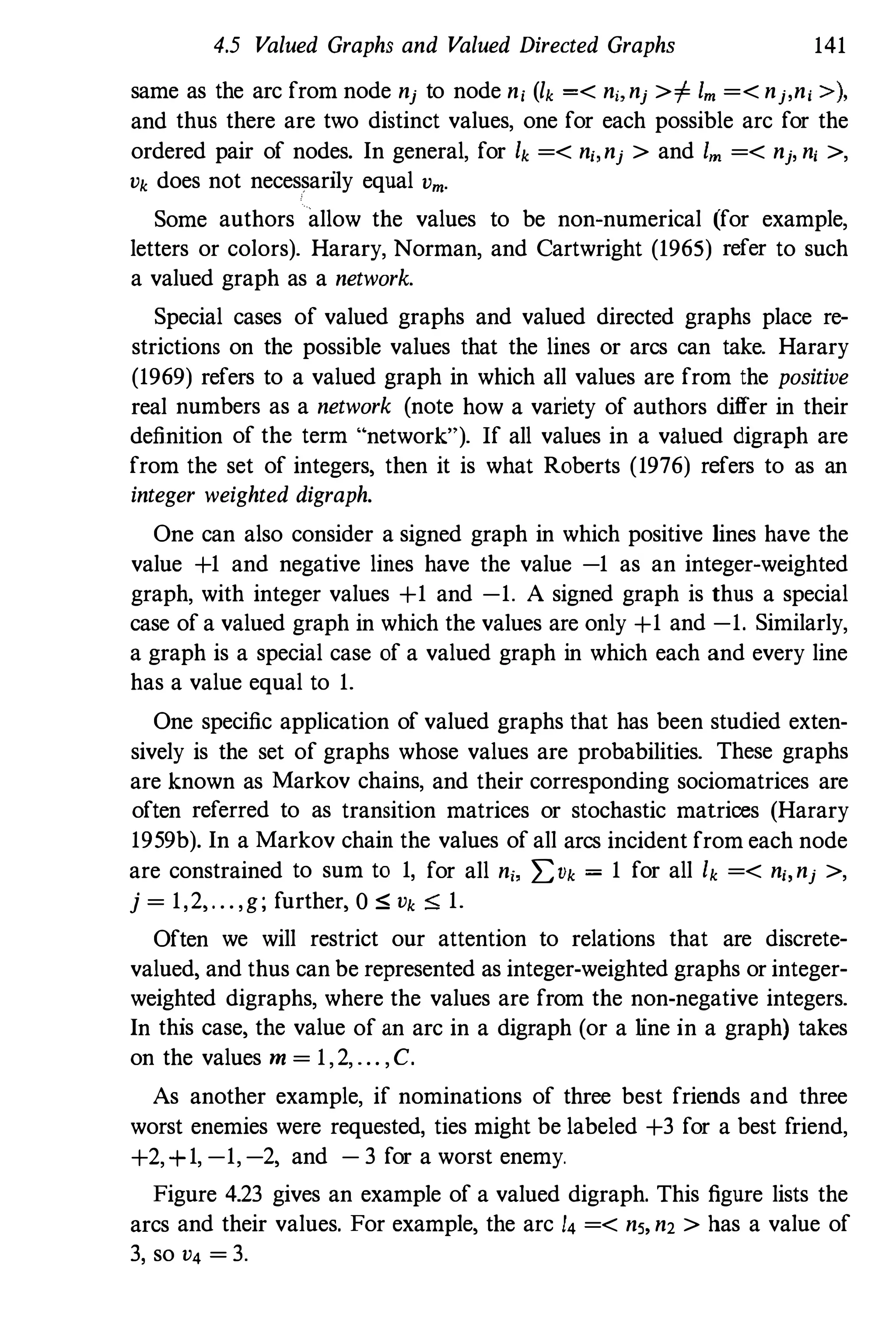
4.2 Graphs 117
also destroy the graph's connectedness, but the minimum number of lines
whose removal disconnects the graph is I (specifically line 14). If A(�) <': I,
the graph is said to be I-line connected, since I is the minimum number
of lines that must be removed to make the graph disconnected.
The larger the node-connectivity or the line-connectivity of a graph is,
the less vulnerable the graph is to becoming disconnected. We will return
to ideas of connectivity in Chapter 7 and discuss how these ideas can be
used to define cohesive subgroups.
4.2.9 Isomorphic Graphs and Subgraphs
Two graphs, q; and Cfj", are isomorphic if there is a one-to-one mapping
from the nodes of � to the nodes of �' that preserves the adjacency of
nodes.
A one-to-one mapping means that each node in � is mapped to one
(and only one) node in �', and each node in �. is mapped to one (and
only one) node in �. Let us denote nodes in � as JV = {nlo n2,. . . ,ng} and
nodes in �' as JV" = {n;, ni, ... ,n;}. We will use the notation q,(n,) = nZ
to indicate that node n, in � is mapped to node nk in �". The inverse of
this mapping, q,-I, is the mapping that maps node nZ in �" to node n, in
�; q,-I(njJ = n,. Since the mapping is a one-to-one mapping, q,(n,) = nk
if and only if q,-I(nZ) = n,.
The mapping preserves adjacency if nodes that are adjacent in � are
mapped to nodes that are adjacent in �", and nodes that are not adjacent
in � are mapped to nodes that are not adjacent in �", and vice versa.
Formally, two graphs are isomorphic iffor all n" nj E JV and nZ, nj E JV"
there exists a one-to-one mapping, q,(n,) = nZ and q,(nj) = ni such that
1m = (n" nj) E 2 if and only if 10 = (nZ, ni) E 2'. If two nodes are
adjacent in one graph, then the nodes they are mapped to must also be
adjacent in the isomorphic graph.
Consider the two graphs in Figure 4.13. Each graph has g = 6 nodes
and L = 6 lines, and the nodes in each graph are labeled. A labeled graph
is a graph in which the nodes have names or labels attached to them.
The labels may be the names of the actors represented by the nodes,
or they may be numbers or letters distinguishing the nodes. Isomorphic
graphs are indistinguishable except for the labels on the nodes. For
example, Figure 4.13a contains a graph �* that is isomorphic to that in
Figure 4.13b, �.
Isomorphisms between graphs are important because iftwo graphs are
isomorphic, then they are identical on all graph theoretic properties. For
118 Graphs and Matrices
�+
�(nl) = Keith
�(n,) = Eliot
�(n3) = Sarah
¢(n4) = Allison
¢(ns) = Drew
¢(n6) = Ross
Fig. 4.13. Isomorphic graphs
Sarah
Ross
Allison
rrew
Eliot
Keith
�
example, two isomorphic graphs have the same number of nodes, the
same number of lines, the same density, the same diameter, and so on.
Thus, if we know that a particular graph theoretic property holds for
graph '1J then we know that the property holds for any graph '1J' that is
isomorphic to '1J.
It is also important to consider the nodes in isomorphic graphs. If
two graphs '1J and '1J' are isomorphic, and ni in graph '1J is mapped to
node nZ in '1J', (</>(ni) = nZ) then ni and nk are identical with respect to all
graph theoretic properties (they have the same nodal degree, the same
eccentricity, and so on). This property is quite important in defining
some kinds of positional equivalences that we discuss in Chapter 12.
We can also consider isomorphic subgraphs. Two subgraphs, '1J, and
'1J;, are isomorphic if there is a one-to-one mapping from the nodes of
'1J, to the nodes of '1J; that preserves the adjacency of nodes (as defined
above). Subgraphs that are isomorphic belong to the same isomorphism
class. Studies of dyads (Chapter 14) and triads (Chapter 15) rely on the
isomorphism of very small subgraphs.
We now consider graphs with special properties.
4.2 Graphs 1 19
> �
a. Cyclic graph b.Tree C. Forest
Fig. 4.14. Cyclic and acyclic graphs
4.2.10 OSpecia/ Kinds ofGraphs
Complement. The complement, <g, of a graph, '#, has the same
set of nodes as '#, a line is present between an unordered pair of nodes
in <g ifthe unordered pair is not in the set of lines in '#, and a line is not
present in <g if it is present in '#. In other words, if nodes n, and nj are
adjacent in '#, then n, and nj are not adjacent in <g, and if nodes n, and
nj are not adjacent in '#, then n, and nj are adjacent in <g. The line sets
for these two graphs have no intersection at all, and their union is the
set of all possible lines (all unordered pairs of nodes).
Trees. A graph that is connected and is acyclic (contains no
cycles) is called a tree. In some ways trees are rather simple graphs, since
they contain the minimum number oflines necessary to be connected, and
they do not contain cycles. Several characteristics oftrees are particularly
important. First, trees are minimally connected graphs since every line in
the graph is a bridge (or line cut). The removal of any one line causes the
graph to be disconnected. Second, the number of lines in a tree equals
the number of nodes minus one (L = g - 1). Adding another line adds a
cycle to the graph, and hence the graph is no longer a tree. Third, there
is only one path between any two nodes in a tree. If this is not true, the
graph contains a cycle, which by definition a tree does not contain.
A graph that is disconnected (has more than one component) and
contains no cycles is called aforest. In a forest, each component is a tree.
120 Graphs and Matrices
Bipartite
Fig. 4.15. Bipartite graphs
Complete bipartite
In general, the number of lines in a tree or forest equals the number
of nodes minus the number of components of the graph. So, L equals g
minus the number of components of <'§. For a tree L = g - 1 since the
number of components for a tree is I.
The graph in Figure 4.14b is a tree. It is easy to verify that each pair
ofnodes is connected via some path, and the graph is acyclic. The graph
in Figure 4.14a is not a tree, because it contains a cycle. The graph in
Figure 4.14c is a forest. In the forest in Figure 4.14c, L = 5, or g minus
2 components.
Bipartite Graphs. Ifthe nodes in a graph can be partitioned into
two subsets, .;V, and .;V2, so that every line in :t' is an unordered pair
of nodes in which one node is in .;V, and the other node is in .;V2, then
the graph is bipartite. In a bipartite graph there are two subsets of nodes
and all lines are between nodes belonging to different subsets. Nodes in
a given subset are adjacent to nodes from the other subset, but no node
is adjacent to any node in its own subset.
A complete bipartite graph is a bipartite graph in which every node
in .;V, is adjacent to every node in ';v2. Complete bipartite graphs are
usually denoted Kgj,g2' where gl is the number of nodes in .%1, and g2 is
the number of nodes in .;V2.
An example of a bipartite graph and a complete bipartite graph is
given in Figure 4.15. Nodes n, and n2 belong to .;V, = {nlo n2} and nodes
n3, n4,nS belong to %2 = {n3,n4,nS}.
A two-mode network with two sets of actors and a relation linking
actors in one set to actors in the second set can be represented as a
bipartite graph. But a bipartite graph may also exist in a one-mode
network. A graph of an exogamous marriage system is bipartite, if, for
example, women from clan A take husbands frilm clan B, and men from
4.3 Directed Graphs 121
clan B take wives from clan A. In that case, all marriages unite partners
from different clans.
The partitioning of the nodes in a graph can be generalized from two
subsets %1 and %2 to s subsets %)'%2, " " %" An s-partite graph is
one in which there is a partitioning ofthe nodes into s subsets so that all
lines are between a node in .Af'i and a node in ,¥j, where i + j. All tines
are between nodes in different subsets and no nodes in the same subset
are adjacent.
The notion of a complete bipartite graph can also be extended to a
complete s-partite graph. A graph is a complete s-partite graph if all
pairs of nodes belonging to different subsets are adjacent. All possible
between-subset lines are present, and there are no lines incident with two
nodes belonging to the same subset (equivalently, no nodes in the same
subset are adjacent).
An example of a network that might be described by a bipartite graph
is the set of monetary donations transacted between corporations in a
specific geographic area, and the non-profit organizations headquartered
in this area. We initially place all firms, both corporations and non­
profit organizations, into a single actor set, %. We then measure the
flows of donations among these firms. Since the non-profit organizations
usually have limited cash resources and thus can not support themselves
financially, they must rely on the corporations for donations. We find
that the only lines in this graph connect corporations to non-profit
organizations. Thus, we have a bipartite graph, with the corporations
n::siding in sel %1 and non-profit organizations in set %2_
Thus far, we have focused our discussion on graphs, where a line
between nodes is either present or absent. As we have emphasized
before, graphs are useful for representing nondirectional relations. In the
next section we discuss directed graphs, which are used for representing
directional relations.
4.3 Directed Graphs
Many relations are directional. A relation is directional if the ties are
oriented from one actor to another. The import/export of goods between
nations is an example of a directional relation. Clearly goods go from
one nation to another; one nation is the source and the other is the
destination of the goods. In a social network representing trade among
nations, the ties are directional and the graph representing such ties must
be directed. Choices of friendships among children are another example
122 Graphs and Matrices
of a directional relation. The claim of friendship is directed from one
child to another child. Child i may choose child j as a friend, but that
does not necessarily imply child j chooses child i as a friend.
In this section we define a directed graph and describe those definitions
and concepts for directed graphs that are most useful for social network
analysis. We refer the reader to Hage and Harary (1983), Harary,
Norman, and Cartwright (1965), or other graph theory reference books
for further discussion of directed graphs.
A directional relation can be represented by a directed graph, or digraph
for short. A digraph consists of a set of nodes representing the actors in
a network, and a set of arcs directed between pairs of nodes representing
directed ties between actors. The difference between a graph and a
directed graph is that in a directed graph the direction of the lines is
specified. Directed ties between the pairs of actors are represented as
lines in which the orientation of the relation is specified. These oriented
lines are called arcs.
A directed graph, or digraph, �d(%, 2), consists of two sets of in­
formation: a set of nodes % = {n"n" . . ., n,}, and a set of arcs, 2 =
{I" 1" . . . , IL}. Each arc is an ordered pair of distinct nodes, Ik =< ni, nJ >.
The arc < ni,nj > is directed from ni (the origin or sender) to nj (the
terminus or receiver). The difference between an arc (in a digraph) and a
line (in a graph) is that an arc is an ordered pair of nodes (to reflect the
direction ofthe tie between the two nodes) whereas a line is an unordered
pair ofnodes (it simply records the presence of a tie between two nodes).
We let L be the number of arcs in 2. Since each arc is an ordered
pair of nodes, there are g(g - 1) possible arcs in 2.
As in a graph, a node is incident with an arc if the node is in the
ordered pair of nodes defining the arc. For example, both nodes ni and
nj are incident with the arc h =< nj. nj >. However, in a digraph, since
an arc is an ordered pair of nodes, we can distinguish the first from the
second node in the pair. Thus, the concept ofadjacency of pairs of nodes
in a digraph is somewhat more complicated than adjacency of pairs of
nodes in a graph. We must consider whether a given node is first (sender)
or second (receiver) in the ordered pair defining the arc. Specifically,
node nj is adjacent to node nj if < ni, nj >E .P, and node nj is adjacent
from node nj if < ni, nj >E P.
When a digraph is presented as a diagram the nodes are represented as
points and the arcs are represented as directed arrows. The arc < ni, nj >
is represented by an arrow from the point representing ni to the point
representing nj. For example, if actor i nominates actor j as a friend,
4.3 Directed Graphs
Actor Likes at beginning of year
"1 Allison Drew Ross
"2 Drew Eliot Sarah
., Eliot Drew
'" Keith Ross
"5 Ross Sarah
"6 Sarah Drew
Allison
�Sarah • �----,I----------- . Drew
Ross .
�Keith
it = (nl,nZ)
h = (nl,ns)
13 = (nZ,n3)
4 � (n2' "6)
15 = (n3,nz)
16 = (n4,ns)
h = (ns,n6)
18 = (n6, nz)
• Eliot
Fig. 4.16. Friendship at the beginning of the year for six children
123
there would be an arc originating at i and terminating at j. If actor
j returned the friendship choice, there would be another arc, this one
originating at j and terminating at i.
To illustrate a directed graph let us consider the choices of friendship
among our six children at the beginning of the year. These choices
are represented in the directed graph in Figure 4.16. The g = 6 nodes
represent the six children, and the arcs represent friendship nominations.
So, there is an arc from one node to another if the child represented by
the first node chose the child represented by the second node as a friend.
For example Ross, ns, chose Sarah, n6, as a friend, so the arc < ns, n6 >
is included in the graph.
124 Graphs and Matrices
Many concepts for graphs (such as subgraph) presented and defined
earlier in this chapter are inunediately applicable to directed graphs, and
thus do not require special discussion. However, some concepts, such
as isomorphism classes for dyads and triads, nodal degree, walks, and
paths are somewhat different in directed graphs, and thus need special
discussion. We now turn to these digraph topics.
4.3.1 Subgraphs - Dyads
One of the most important subgraphs in a digraph is the dyad, consisting
of two nodes and the possible arcs between them. Since there may or
may not be an arc in either direction for a pair of nodes, n, and nj, there
are four possible states for each dyad. However, there are only three
isomorphism classes (all dyads are identical to one of these three types).
The first isomorphism class of a dyad is the null dyad. Null dyads
have no arcs, in either direction, between the two nodes. The dyad for
nodes ni and nj is null if neither of the arcs < nj, nj > nor < ni' nj > is
contained in the set of arcs, 2". The second isomorphism class is called
asymmetric. An asymmetric dyad has an arc between the two nodes going
in one direction or the other, but not both. The dyad for nodes n, and
nj is asymmetric if either one of the arcs < ni, nj > or < nj,ni >, but
not both, is contained in the set of arcs, 2". Thus, there are two possible
asymmetric dyads, but they are isomorphic. The third isomorphism
class is called a mutual or reciprocal dyad. Mutual dyads have two arcs
between the nodes, one going in one direction and the other going in the
opposite direction. The dyad for nodes n, and nj is mutual if both arcs
< ni,nj > and < njl nj > are contained in the set of arcs, 2. Thus the
three isomorphism classes for dyads are: nulL asynunetric, and mutual.
If the directed graph represents the friendship relation, a null dyad is
one in which neither person chooses the other. The asymmetric dyad
occurs when one person chooses the other, without the choice being
reciprocated. In a mutual dyad both actors in the pair choose each other
as friends.
Figure 4.17 shows the dyads for the example of friendships at the
beginning of the year among the six children (presented in Figure 4.16).
Since there are g = 6 children, there are 6(5 - 1)/2 = 15 dyads to
consider. Figure 4.17 shows the state of each of these 15 dyads.
The arc with a double-headed arrow between n2 and n3 indicates a
mutual dyad. Asymmetric dyads are represented by one-way arcs, such
4.3 Directed Graphs 125
n, � n2 (asymmetric)
n, n, (null)
n, n4 (null)
n, � n, (asymmetric)
n, n, (null)
n2 +-----> n, (mutual)
n, n, (null)
n, n, (null)
n, +-----> n, (mutual)
n, n4 (null)
n, n, (null)
n, n, (null)
n4 � n, (asymmetric)
n4 n, (null)
n, � n, (asymmetric)
Fig. 4.17. Dyads from the graph of friendship among six children at
the beginning of the year
as from nl to n2. The dyad involving Allison, nl, and Keith, n4, is a null
dyad, since neither arc is present.
The kinds of dyads that arise in a directed graph are quite interesting
and important for describing a social network. Tendencies for reciprocity
(mutuality) and/or asymmetry in a digraph are often summarized by
counting the number of dyads in each of the three isomorphism classes.
Chapter 13 discusses these ideas and presents some models for dyads.
One could 'tndy 'nhgraph' ofany ,ize for a digraph. Dyads are clearly
subgraphs of size two. Triads, subgraphs ofsize three, are important for
studying ideas such as balance, clusterability, and transitivity (which we
describe in detail in Chapter 6). Cohesive subgroups are also studied by
focusing on subgroups (see Chapter 7).
We now discuss how several of the concepts for graphs are applied
to directed graphs. We will focus on the most important directed graph
concepts including the nodal degrees, walks, paths, reachability, and
connectivity.
4.3.2 Nodal Indegree and OUldegree
In a graph, the degree of a node is the number of nodes adjacent to it
(equivalently, the number of lines incident with it). In a digraph, a node
can be either adjacent to, or adjacent from another node, depending on
the "direction" of the arc. Thus, it is necessary to consider these cases
126 Graphs and Matrices
separately. One quantifies the tendency of actors to make "choices"; the
other quantifies the tendency to receive "choices."
The indegree of a node, dl(ni), is the number of nodes that are adjacent
to ni. The indegree of node ni is equal to the number of arcs of the form
Ik =< nj,ni >, for all Ik E 2', and all nj E ff. Indegree is thus the
number of arcs terminating at lli.
The outdegree of a node, do(ni), is the number of nodes adjacentfrom
ni. The outdegree of node ni is equal to the number of arcs of the form
Ik =< ni,nj >, for all Ik E 2', and all nj E ff. Outdegree is thus the
number of arcs originating with node ni.
The indegrees and outdegrees for each node may be obtained by
considering the arcs in the digraph. Thus, the outdegrees for the six
nodes, representing children, in Figure 4.16 are:
• doCn.) = 2
• do(n2) = 2
• do(n,) = 1
• doCn,) = 1
• doCn,) = 1
• doCn6) = 1
The indegrees are:
• d/(nd = 0
• d/(n2) = 3
• d/(n,) = 1
• d/(n,) = 0
• d/(n,) = 2
• d/(n6) = 2
In social network applications, these degrees can be of great interest.
The outdegrees are measures of expansiveness and the indegrees are mea­
sures of receptivity, or popularity. If we consider the sociometric relation
of friendship, an actor with a large outdegree is one who nominates
many others as friends. An actor with a small outdegree nominates
fewer friends. An actor with a large indegree is one whom many others
nominate as a friend, and an actor with a small indegree is chosen by
few others. Outdegrees may be fixed by the data collection design, if, for
example, a researcher collects data in which each respondent is instructed
to "name your three closest friends." In such a setting, if all respondents
in fact named three closest friends, then all outdegrees would equal 3.
4.3 Directed Graphs 127
Indegrees and outdegrees are useful measurements for many different
types of networks and relations, although the terms "expansive" and
"popular" may be somewhat inappropriate in some cases. For example,
consider the countries trade network, and the relation "exports manu­
factured goods to" among countries. A country with high outdegree is a
heavy exporter, and a country with high indegree is a heavy importer.
In many statistical models we might want to control for, or condition
on, either the indegrees or the outdegrees ofthe nodes. For example, ifwe
are studying the tendency for mutual choices within a network, we might
control for the nodal outdegrees; that is, we would study the tendency
for mutuality, given the propensity of our actors to make choices. Such
statistical conditioning is used in Chapters 13�16.
It is often useful to summarize the indegrees and!or the outdegrees
of all the actors in the network using the mean indegree or the mean
outdegree. As we will see, these two numbers are equal, since they are
considering the same set of arcs, but from different "directions." We will
denote the mean indegree as dI, and the mean outdegree as do. These
are calculated as:
dI �f�l dI(ni)
g
do
�f�l do(ni)
g
(4.6)
Since tbe indegrees count arcs incident from the nodes, and the outdegree
count arcs incident to the nodes, �f�l dI(ni) = �f�l do(ni) = L, and thus
we can see that dI = do and equations (4.6) simplify to:
- L
do = - .
g
(4.7)
One might also be interested in the variability of the nodal indegrees
and outdegrees. Unlike the mean indegree and the mean outdegree, the
variance of the indegrees is not necessarily the same as the variance of
the outdegrees. For example, consider a sociometric question in which
each person is asked to name her three closest friends. If all people in
fact make three nominations, then there is no variance in the outdegrees
(all do(n;l = 3). However, it is likely that people will receive different
numbers of "choices"; thus, there will be variability in the indegrees (the
dI(ni)'s will differ from each other). The variance of the indegrees, which
we denote by St" , is calculated as:
128 Graphs and Matrices
",g ) - 2
S
2 _ L.d_,(d/(n, - d/)
D/ - g
. (4.8)
Similarly, the variance of the outdegrees, which we denote by SEa' is
calculated as:
(4.9)
Both of these measures quantify how unequal the actors in a network
are with respect to initiating or receiving ties. These measures are simple
statistics for summarizing how "centralized" a network is. We return to
this idea in Chapter 5.
Types of Nodes in a Directed Graph. The indegrees and outde­
grees of the nodes in a directed graph can be used to distinguish four
different kinds of nodes based on the possible ways that arcs can be
incident with the node. Recall that the indegree of node n" denoted by
dI(n,), is equal to the number of nodes adjacent to it, and the outdegree
of node n" denoted by do(n,), is equal to the number of nodes adjacent
from it. In terms of the indegree and outdegree there are four possible
kinds ofnodes: the node is an isolate, the node only has arcs originating
from it, the node only has arcs terminating at it, or the node has arcs
both to and from it. Graph theorists provide a vocabulary for labeling
these four kinds of nodes (Harary, Norman, and Cartwright 1965, page
18; Hage and Harary 1983). According to this classification, a node is
a(n):
• Isolate if d/(n,) = do(n,) = 0,
• Transmitter if d/(n,) = 0 and do(n,) > 0,
• Receiver if dI(n,) > 0 and do(n,) = 0,
• Carrier or ordinary if d1(n,) > 0 and do(n,) > 0
The distinction between a carrier and an ordinary node is that, although
both kinds have both positive indegree and positive outdegree, a carrier
has both indegree and outdegree precisely equal to 1, whereas an ordinary
node has indegree and/or outdegree greater than 1.
Several authors have argued that this typology, or some variant of
it, is useful for describing the "roles" or "positions" of actors in social
networks (Burt 1976; Marsden 1989; Richards 1989a).
4.3 Directed Graphs 129
4.3.3 Density of a Directed Graph
The density of a directed graph is equal to the proportion of arcs present
in the digraph. It is calculated as the number of arcs, L, divided by the
possible number of arcs. Since an arc is an ordered pair of nodes, there
are g(g - 1) possible arcs. The density, fl, is:
fl =
L
g(g - 1)
(4.10)
The density of a digraph is a fraction that goes from a minimum of 0,
if no arcs are present, to a maximum of 1, if all arcs are present. If the
density is equal to 1, then all dyads are mutual.
4.3.4 An Example
Now let us illustrate nodal indegree and outdegree, and the density of a
directed graph on the example of friendships among Krackhardt's high­
tech managers. Clearly a directed graph is the appropriate representation
for these friendship choices, since each choice of friendship is directed
from one manager to another (and is not necessarily reciprocated).
Table 4.1 presents the nodal indegrees and outdegrees, the mean and
variance of the indegrees and outdegrees, and the density of the graph.
From these results we see that there are no isolates in this network (there
are no managers with both indegree and outdegree eqnal to 0). However,
there are two managers (managers 7 and 9) who did not make any
friendship nominations. The mean number of friendship choices made
(and received) is equal to 4.86. The density of the relation is equal to
0.243.
4.3.5 Directed Walks, Paths, Semipaths
Walks and related concepts in graphs can also be defined for digraphs,
but one must consider the direction of the arcs. We first define directed
walks, directed paths, and semipaths for directed graphs and then define
closed walks (cycles and semicycles) for directed graphs.
A directed walk is a sequence of alternating nodes and arcs so that
each arc has its origin at the previous node and its terminus at the
subsequent node. More simply, in a directed walk, all arcs are "pointing"
in the same direction. The length of a directed walk is the number of
instances of arcs in it (an arc is counted each time it occurs in the walk).
130 Graphs and Matrices
Table 4.1. Nodal degree and density forfriendships among Krackhardt's
high-tech managers
Manager Indegree Outdegree
L � 102
g � 21
1 8 5
2 10 3
3 5 2
4 5 6
5 6 7
6 2 6
7 3 0
8 5 1
9 6 0
10 1 7
11 6 13
12 8 4
13 1 2
14 5 2
15 4 8
16 4 2
17 6 18
18 4 1
19 5 9
20 3 2
21 5 4
dI � do � 102/21 � 4.86
possible number of arcs: 21(20) � 420
!J. � 102/420 � 0.243
S�l = 2.172
S�o = 4.372
For example, consider the digraph in Figure 4.18. One directed walk
in this figure is W = n5nln2n3n4n2n3.
Recall that a trail in a graph is a walk in which no line is inclnded
more than once. A directed trail in a digraph is a directed walk in which
no arc is included more than once. Similarly, a directed path or simply
a path iIi a digraph is a directed walk in which no node and no arc is
included more than once. A path joining nodes ni and nj in a directed
graph is a sequence of distinct nodes, where each arc has its origin at the
previous node, and its ten:rrinus at the subsequent node. Thus, a path
in a directed graph consists of arcs all "pointing" in the same direction.
The length of a path is the number of arcs in it.
4.3 Di�ected Graphs
�
r.�------e n,
Directed walk ns nl tiz n3 n4 n2 n3
Directed path tis »4 m n3
Semipath nl ti2 tis n4 n3
Cycle ti2 ti3 »4 n2
Semicycle nl n2 ns nl
Fig. 4.18. Directed walks. paths, semipaths, and semicycles
131
Now, consider removing the restriction that all arcs "point" in the
same direction. We will simply consider walks and paths in which the
arc between previous and subsequent nodes in the sequence may go in
either direction. A semiwalk joining nodes n, and nj is a sequence of
nodes and arcs in which successive pairs of nodes are incident with an
arc from the first to the second, or by an arc from the second to the first.
That is, in a semiwalk, for all successive pairs of nodes, the arc between
adjacent nodes may be either < nj, nj > or < nj. nj >. In a semiwalk
the direction of the arcs is irrelevant. The length of a semiwalk is the
number of instances of arcs in it.
A semipath joining nodes n, and nj is a sequence of distinct nodes,
where all successive pairs of nodes are connected by an arc from the first
.
to the second, or by an arc from the second to the first for all successive
pairs of nodes (Harary, Norman, and Cartwright 1965; Peay 1975). In a
semipath the direction of the arcs is irrelevant. The length of a semipath
is the number of arcs in it.
Note that every path is a semipath, but not every semipath is a path
(see Harary, Norman, and Cartwright 1965, for more discussion).
Closed walks can also be defined for directed graphs. A cycle in a
directed graph is a closed directed walk of at least three nodes in which
all nodes except the first and last are distinct. A semicycle in a directed
graph is a closed directed semiwalk of at least three nodes in which all
132 Graphs and Matrices
nodes except the first and last are distinct. In a semicycle the arcs may
go in either direction, whereas in a cycle the arcs must all "point" in
the Same direction. Semicycles are used to study structural balance and
clusterability (see Chapter 6).
Figure 4.18 gives examples of a directed walk, a directed path, a
semipath, a cycle, and a semicyc1e.
4.3.6 Reachability and Connectivity in Digraphs
Using the ideas of paths and semipaths, we can now define reachability
and connectivity of pairs of nodes, and the connectedness of a directed
graph.
Pairs of Nodes. In a graph a pair of nodes is reachable if there
is a path between them. However, in order to define reachability in a
directed graph, we must consider directed paths. Specifically, if there is a
directed path from n, to nj, then node nj is reachable from node n,.
Consider now both paths and semipaths between pairs of nodes. We
can define four different ways that two nodes can be connected by a
path, or semipath (Harary, Norman, and Cartwright 1965; Frank 1971;
Peay 1975, 1980). A pair of nodes, n" nj, is:
(i) Weakly connected if they are joined by a semipath
(ii) Unilaterally connected if they are joined by a path from n, to nj,
or a path from nj to nj
(iii) Strongly connected if there is a path from n, to nj, and a path
from nj to n,; the path from n, to nj may contain different nodes
and arcs than the path from nj to n,
(iv) Recursively connected if they are strongly connected, and the
path from n, to nj uses the same nodes and arcs as the path
from nj to nj, in reverse order
Notice that these forms of connectivity are increasingly strict, and
that any strict form implies connectivity of any less strict form. For
example, any two nodes that are recursively connected are also strongly
connected, unilaterally connected, and weakly connected. Figure 4.19
illustrates these different kinds ofconnectivity. In each case nodes nl and
n4 in the graph demonstrate the different versions of connectivity.
4.3 Directed Graphs
•
1 ! •
2
I. 3 ! • 4 Unilateral
1 �
-<"�2 , �4 Strong
1 2 3
••�'---4.t+. -�'·4.t+.-�,�•• 4 Recursive
Fig. 4.19. Different kinds of connectivity in a directed graph
133
Digrapb Connec4edness. Itis now possible to define four different
kinds of connectivity for digraphs (Peay 1975, 1980). If a digraph is
connected, then it is connected by one ofthese four kinds of connectivity;
otherwise, it is not connected. Since there are four types of connectivity
between pairs of nodes in a directed graph, there are four definitions of
graph connectivity for a digraph. A directed graph is:
(i) Weakly connected if all pairs of nodes are weakly connected
(ii) Unilaterally connected if all pairs of nodes are unilaterally con­
nected
(iii) Strongly connected if all pairs of nodes are strongly connected
(iv) Recursively connected if all pairs of nodes are recursively con­
nected
In a weakly connected digraph, all pairs of nodes are connected by
a semipath. In a unilaterally connected digraph, between each pair of
nodes there is a directed path from one node to the other; in other
words at least one node is reachable from the other in the pair. In a
strongly connected digraph each node in each pair is reachable from the
other; there is a directed path from each node to each other node. In a
recursively connected digraph, each node, in each pair, is reachable from
the other, and the directed paths contain the same nodes and arcs, but in
reverse order. As with the definitions of connectivity for pairs of nodes,
these are increasingly strict graph connectivity definitions.
From these definitions it should be clear that every strongly connected
digraph is unilaterally connected, but the reverse is not true. When
134 Graphs and Matrices
maximal subgraphs are derived from digraphs in which the actors are
unilaterally, or strongly, connected, the subgraph is referred to as a
unilateral, or strong, component in the digraph. These ideas are used to
study cohesive subgroups in directed graphs (see Chapter 7).
4.3.7 Geodesics, Distance and Diameter
The (geodesic) distance between a pair of nodes in a graph is the length
of a shortest path between the two nodes, and is the basis for defining
the diameter of the graph. In a directed graph, the paths from node
n, to node nj may be different from the paths from node nj to node n,
(because paths in a directed graph consider the direction of the arcs).
Thus, the definitions of distance and diameter in a directed graph are
somewhat more complicated than in a graph.
Consider the paths from node n, to node nj. A geodesic from node n,
to node nj is a shortest pathfrom n, to nj. The distance from n, to nj,
denoted by d(i,j), is the length ofa geodesic from n, to nj. It is important
to note that since the paths from n, are likely to be different from the
paths from nj to n, (since paths require that all arcs are "pointing" in
the same direction) the geodesics from n, to nj may be different from
the geodesics from nj to n,. Thus, the distance, d(i,j), from n, to nj may
be different from the distance, d(j, i), from nj to n,. For example, in
Figure 4.18 d(4,2) = 1 whereas d(2, 4) = 2. If there is no path from n, to
nj (as might be the case when the graph is only weakly or unilaterally
connected) then there is no geodesic from n, to nj, and the distance from
n, to nj is undefined (or infinite).
Now, consider the diameter of a directed graph. As in a graph, the
diameter ofa directed graph is the length ofthe longest geodesic between
any pair of nodes. This definition of geodesic is useful if there is a path
from each node to each other node in the graph; that is, the graph
is strongly connected or recursively connected. However, if the graph
is only unilaterally or weakly connected, then, as noted above, some
distances are undefined (or infinite). Thus, the diameter of a weakly or
unilaterally connected directed graph is undefined.
4.3.8 OSpecia/ Kinds ofDirected Graphs
In this section we describe several kinds of digraphs with important
properties. We begin by defining digraph complement and digraph
converse.
4.3 Directed Graphs 135
n, n2 n, n2 n, n2
X rsJ Xn, n3 n, n3 n4 n3
q/d q/d q/'d
Graph Complement Converse
Fig. 4.20. Converse and complement of a directed graph
Complement and Converse of a Digraph. Now let us consider
two kinds of digraphs that can be derived from a digraph. These derived
digraphs can be used to represent the opposite and the negation of a
relation.
The complement, qjd, of a directed graph, 'lid, has the same set of nodes
as q;d, but there is an arc present between an ordered pair of nodes in
qjd if the ordered pair is not in the set of arcs in 'lid, and an arc is not
present in qjd if it is present in 'lid. In other words, if the arc < n" nj > is
in '!ld, then the arc < nj,nj > is not in ?gd, and if the arc < ni,nj > is not
in '!ld, then the arc < nilnj > is in "?gd.
The converse, 'lid' of a directed graph, 'lid, has the same set of nodes
as qjd. but the arc < ni,nj > is in <§d only if the arc < nj, nj > is in qjd
(Harary 1969). The converse, 'lid' is obtained from 'lid by reversing the
direction of all arcs. The arcs in the converse connect the same pairs of
nodes as the arcs in the digraph, but all arcs are reversed in direction.
That is, an arc in the digraph from n, to nj becomes an arc in the
converse from nj to n,. Figure 4.20 shows a directed graph, its converse,
and its complement.
The converse of a directed graph might be helpful in thinking about
relations that have "opposites." For example, the converse of a digraph
representing a dominance relation (for example, n, "wins over" nj) would
represent the submissive relation (nj "loses to" n,). On the other hand,
the complement of a digraph might be used to represent the absence of
a tie, or as not the relation. For example, in the digraph representing the
relation of friendship the arc < n" nj > means i "chooses" j as a friend.
In the digraph representing the complement of the relation of friendship,
the arc < ni, nj > means i "does not choose" j as a friend.
136 Graphs and Matrices
Tournaments. One other special type of a digraph is a tourna­
ment, which mathematically represents a set of actors competing in some
event(s) and a relation indicating superior performances or "beats" in
competition (see Moon 1968). Ifteam n; beats team nj, an arc is directed
from ni toward nj. Of particular interest are round-robin tournaments,
where each team plays each other team exactly once. Such tourna­
ments can be modeled as round robin designs (Kenny 1981; Kenny and
LaYoie 1984; Wong 1982). These competitive records form a special type
of digraph, because each pair of nodes is connected by exactly one arc.
Methodology for such designs is related to the Bradley-Terry-Luce model
for paired comparisons, which allows for statistical estimation of popu­
lation propensities for dominance (Bradley and Terry 1952; Thurstone
1927; Coombs 1951; Mosteller 1951; Frank 1981; and David 1988).
4.3.9 Summary
Digraphs are the appropriate representation of social networks in which
relations are dichotomous (ties are either present or absent) and direc­
tional. However, many relations are valued; that is, the ties indicate the
strength or intensity ofthe tie between each pair of actors. Thus, we need
to generalize both graphs and directed graphs so that we can represent
the strength of ties between actors in a network. The graph for a valued
relation must convey more information by representing the strength of
an arc or a line. For example, observations of the number of interactions
between pairs of people in a group require valued relations. Similarly,
ratings of friendship in which people distinguish between "close personal
friends," "friends," "acquaintances," and "strangers" must be represented
by a graph in which the arcs also have a value indicating the strength
of the tie. In the next sections we define and discuss signed graphs (in
which the lines or arcs take on a positive or negative sign). In the section
following that we discuss valued graphs (in which the lines or arcs can
take on a values from the real numbers).
4.4 Signed Graphs and Signed Directed Graphs
Occasionally relations are measured in which the ties can be interpreted
as heing either positive Or negative in affect, evaluation, or meaning. For
example, one might measure the relations "loves" and "hates" among the
people in a group, or the relations "is allied with" and "is at war with"
among countries. Such relations can be represented as a signed graph,
4.4 Signed Graphs and Signed Directed Graphs 137
or as a signed directed graph. We begin by defining a signed graph, and
then generalize to a signed directed graph. Signed graphs and signed
directed graphs are important in the study of balance and clusterability
(discussed in Chapter 6).
4.4.1 Signed Graph
A signed graph is a graph whose lines carry the additional information
of a valence: a positive or negative sign. A signed graph consists of three
sets of information: a set of nodes, .;V = {nl, n2, . . . ,ng}, a set of lines,
:.e = {l1,l2, ... , ld, and a set of valences (or signs), l' = {vlov2,. . .,vd,
attached to the lines. As usual, each line is an unordered pair of distinct
nodes, h = (ni,nj). But now, associated with each line is a valence, Vk
either "+" or "-". A line, Ik = (ni, nj) is assigned the valence Vk = +
if the tie between actors i and j is positive in meaning or affect, and a
valence Vk = - if the tie between the actors represented by the nodes is
negative. We denote a signed graph as �±(.;V, :.e, 1'), or simply �±.
For example, we can represent alliances and hostilities among nations
using a signed graph by letting nodes represent countries, and letting
signed lines represent whether pairs of countries are at war with each
other, "-", or have a treaty with each other, "+",
A complete signed graph is a signed graph in which all unordered pairs
of nodes are included in the set of lines. Since all lines are present in a
complete signed graph, and all lines have a valence either "+" or "-",
each unordered pair of nodes is assigned either "+" or "'-".
Dyads and Triads. In a signed graph, each dyad is in one of
three states: There is a positive line between them, there is a negative line
between them, or there is no line between them. In a complete signed
graph each dyad is in one of two states, either "+" or "-".
In a complete signed graph, a triad may be in one of four possible
states,depending on whetherzero, one, two, or three positive (or negative)
lines are present among the three nodes.
Cycles. Many properties of signed graphs (such as balance and
clusterability) depend on cycles and properties of cycles. In this section
we define the sign of a cycle in a signed graph. Recall that a cycle is a
closed walk in which all nodes except the beginning and ending node are
distinct. Notice that each line in a cycle in a signed graph is either "+"
or "-". In a signed graph, the sign of a cycle is defined as the product of
138 Graphs and Matrices
", e'-----f�-----...,.n2
n4
It = (ni nz) VI = -
lz = (nI n3) V2 = +
h = (nI n4) V3 = +
4 � (n1 n,) V4 = -
15 = (n2 n3) vS = -
16 = (m ns) V6 = -
17 = (n3 n4) V7 = +
Cycle Sign of cycle
nl n2 ns nl - x - x - = -
n3 n4 ni n3 + x + x + = +
ni n2 n3 ni - x - x + = +
Fig. 4.21. Example of a signed graph
the signs of the lines included in the cycle; where the sign of the product
is defined as;
- (+l(+l = +
- (+l(-) = -
- (-)(-) = +
In brief, if a cycle has an even number of negative, '"-", lines, then its
sign is positive. However, if a cycle has an odd number of negative lines,
its sign is negative.
Figure 4.21 gives an example of a signed graph and some of its cycles.
4.4.2 Signed Directed Graphs
It is straightforward to extend the idea of a signed graph to a signed
directed graph. A signed directed graph is a directed graph in which
4.4 Signed Graphs and Signed Directed Graphs
g =5 children's friends (+)
and enemies (-)
Fig. 4.22. Example of a signed directed graph
139
the arc� have the additional information of a positive or negative sign.
A signed digraph consists of three sets of information: a set of nodes,
JV = {nj, n2, . . . , ng}, a set of arcs, !E = {Ib 12, • . • , Id, and a set of
valences, "1' = {Vj,V2, . . ., vd, attached to the arcs. In a signed directed
graph, each arc is an ordered pair of distinct nodes, < n" nj >. Associated
with each arc is a valence, either "+" or "-", Since the arc lk =< ni, nj >
is distinct from the arc 1m =< n" nj >, the sign Vk may be different from
the sign Vm• We can denote a signed directed graph as Wd±(JV, !E, "1'), or
simply Wd±.
Claims of friendship and enmity among people can be represented as
a signed directed graph. Nominations of friends might be represented
by a "+" and nominations of enemies might be represented by a "-".
Figure 4.22 contains an example of a signed digraph, which we can take
to represent such friendship and enmity nominations among people.
Semicycles. In a signed directed graph the most general cycles
are usually referred to as semicycles. Recall that a semicycle is a closed
sequence of distinct nodes and arcs in which each node is either adjacent
to or adjacent from the previous node in the sequence. Thus a semicycle
is a cycle in which the arcs may point in either direction. The sign ofa
semicycle is the product of the signs of the arcs in it.
This idea is important for studying balance and clusterability in signed
directed graphs (see Chapter 6).
Signed graphs and signed directed graphs generalize graphs and di­
rected graphs by allowing the lines or arcs to have valences. Now, let
us generalize even further by allowing the lines or arcs to have other
(usually numerical) values.
140 Graphs and Matrices
4.5 Valued Graphs and Valued Directed Graphs
Often social network data consist ofvalued relations in which the strength
or intensity of each tie is recorded. Examples of valued relations include
the frequency of interaction among pairs of people, the dollar amount
of trade between nations, or the rating of friendship between people in
a group. Such relations cannot be fully represented using a graph or
a directed graph, since lines or arcs in a graph or directed graph are
only present or absent (dichotomous: 0 or 1). Thus, the next step in
the generalization of graphs and digraphs is to add a value or magnitude
to each line or arc. Valued graphs are the appropriate graph theoretic
representation for valued relations. In this section we define and describe
valued graphs.
There are several special valued graphs; for example, weighted graphs
and integer weighted graphs (Roberts 1976), nets and networks (Rarary
1969), and Markov chains. We will briefly describe each. Concepts
and definitions for valued graphs are not as well developed as they
are for graphs and directed graphs; thus, our discussion of valued
graphs will be briefer than our discussion of graphs and directed
graphs.
A valued graph or a valued directed graph is a graph (or digraph) in
which each line (or arc) carries a value. A valued graph consists of three
sets of information: a set of nodes, JV = {nl,n2,. . ., ng}, a set of lines (or
arcs), 2 = {lr,l2, ... , ld, and a set ofvalues, 1/" = {vr,V2, · . . ,vd, attached
to the lines (or arcs). Associated with each line (in a graph) or each arc
(in a digraph) is a value from the set of real numbers (Flament 1963). We
denote a valued graph by qjv(JV, 2, 1/"), or simply qjv. Roberts (1976)
refers to a valued digraph as a weighted digraph.
A valued graph represents a nondirectional valued relation, such as
the number of interactions observed between each pair of people in a
group. The number of interactions between actor i and actor j is the
same as the number of interactions between actor j and actor i. In a
valued graph the line between node n, and node nj is identical to the line
between node nj and node n, (lk = (n" nj) = (nj, n,l), and thus there is
only a single value, Vb for each unordered pair of nodes.
A valued directed graph represents a directional valued relation, such
as the dollar amount of manufactured goods exported from each country
to each other country. Country i may export a different amount of
manufactured goods to country j than country j exports to country i.
In a valued directed graph, the arc from node n, to node nj is not the
4.5 Valued Graphs and Valued Directed Graphs 141
same as the arc from node nj to node n, (lk =< n" nj >i= 1m =< nj,n, » ,
and thus there are two distinct values, one for each possible arc for the
ordered pair of nodes. In general, for Ik =< n" nj > and 1m =< nj, n, >,
Vk does not necessarily equal Vm.
Some authors allow the values to be non-numerical (for example,
letters or colors). Harary, Norman, and Cartwright (1965) refer to such
a valued graph as a network.
Special cases of valued graphs and valued directed graphs place re­
strictions on the possible values that the lines or arcs can take. Harary
(1969) refers to a valued graph in which all values are from the positive
real numbers as a network (note how a variety of authors differ in their
definition of the term "network"). If all values in a valued digraph are
from the set of integers, then it is what Roberts (1976) refers to as an
integer weighted digraph.
One can also consider a signed graph in which positive lines have the
value +1 and negative lines have the value -1 as an integer-weighted
graph, with integer values +1 and -1. A signed graph is thus a special
case of a valued graph in which the values are only +1 and -1. Similarly,
a graph is a special case of a valued graph in which each and every line
has a value equal to 1.
One specific application of valued graphs that has been studied exten­
sively is the set of graphs whose values are probabilities. These graphs
are known as Markov chains, and their corresponding sociomatrices are
often referred to as transition matrices or stochastic matrices (Harary
1959b). In a Markov chain the values of all arcs incident from each node
are constrained to sum to 1, for all n" I:Vk = 1 for all Ik =< n" nj >,
j = 1,2,. . . ,g; further, 0 S Vk S 1.
Often we will restrict our attention to relations that are discrete­
valued, and thus can be represented as integer-weighted graphs or integer­
weighted digraphs, where the values are from the non-negative integers.
In this case, the value of an arc in a digraph (or a line in a graph) takes
on the values rn = 1,2, . . . ,C.
As another example, if nominations of three best friends and three
worst enemies were requested, ties might be labeled +3 for a best friend,
+2,+1, -1, -2, and - 3 for a worst enemy.
Figure 4.23 gives an example of a valued digraph. This figure lists the
arcs and their values. For example, the arc 14 =< ns, n2 > has a value of
3, so V4 = 3.
142 Graphs and Matrices
•
",
3
II = < n3,nl >
12 = < nz,n4 >
13 = < 1l4,n3 >
14 = < ns,n2 >
2
VI = 2
V2 = 2
V3 = 1
V4 = 3
n,
•
Fig. 4.23. Example of a valued directed graph
4.5.1 Nodes and Dyads
Nodes in Valued Graphs. Each node in a valued graph can have
a number of lines incident with it. Similarly, each node in a valued
digraph can have a number of arcs incident to it and/or from it. To
each line or arc is attached a value. In a graph or digraph, nodal degree
is equal to the number of lines incident with the node or the number
of arcs incident to it or from it. The idea of degree does not generalize
well to valued graphs, since one must consider the values attached to the
lines.
One way to generalize the notion of degree to valued graphs and
digraphs is to average the values over all lines incident with a node, or
all arcs incident to or from a node. Such a measure refieets the average
value of the lines incident with the node or of the arcs to or from the
node.
Dyads in Valued Graphs. A dyad in a valued graph has a line
between nodes with a specific strength. A dyad in a valued directed
graph has arcs between the nodes. Each of the two arcs < n,.nj > and
< nj, n, > has a value, which we denote by Vk and Vm• These values most
4.5 Valued Graphs and Valued Directed Graphs 143
likely will be different. It is of interest in such settings to compare the Vk
to Vm. Models for such dyads are discussed in Chapter 15.
4.5.2 Density in a Valued Graph
In a graph or digraph. density, LI., is defined as the ratio of the number of
lines or arcs present to the maximum possible that could arise. Another
way to view the density of a graph or a digraph is as the average of the
values assigned to the lines/arcs. Each line or arc is given a value of 1,
and pairs ofnodes for which lines are absent are given a value ofO. The
sum of these values is equal to the number of lines or arcs; one then
divides this sum by its maximum possible value.
To generalize the notion of density to a valued graph or digraph, one
can average the values attached to the lines/arcs across all lines/arcs.
Thus, for a valued graph/digraph, the density is LI. = z=Vk/g(g-l) where
the sum is taken over all k. This measures the average strength of the
lines/arcs in the valued graph/digraph.
4.5.3 OPaths in Valued Graphs
Walks and paths in valued graphs are defined the same way as they are
in graphs (as an alternating sequence of nodes and lines beginning and
ending with nodes). However, in a valued graph (or valued digraph)
since the lines (or arcs) have values attached to them, concepts such as
reachabllity of a pair of nodes, length of a path, and distance between a
pair ofnodes become more complicated. In order to define these concepts
for valued graphs, we must consider the values attached to each of the
lines (or arcs) in a path. As Peay (1980) has noted, there are a number
of different, and reasonable, ways to define distance and values for paths
in a valued graph. The choice of which definition to use depends on the
interpretation of the lines (arcs) and values in the graph. As in a graph,
nodes ni and nj are reachable if there is a path between them. In a valued
graph we can also consider "strengths" or "values" of reachability.
Value of a Path. The value of a path (semipath) is equal to the
smallest value attached to any line (arc) in it (Peay 1980). Formally,
the value of W = I"I" . . ., lk from ni to nj equals min(v"v" . . . , Vk). The
value of a path is thus the "weakest link" in the path. This idea makes
most sense if larger values indicate stronger ties. For example, ifthe lines
represent the amount of communication between each pair of people in
144 Graphs and Matrices
a group, then the value of a path between two people represents the
most "restricted" amount of communication between any pair of people
in the path.
Now, for simplicity, consider a valued graph in which the values
attached to the lines are discrete and ordinal, and take on values 1, 2,. . ., C
(this is a simplifying condition that is not necessary). We define a path
at level c as a path between a pair of nodes such that each and every
line in the path has a value greater than or equal to c; that is, v/ ;e: c
for all v/ in the path (Doreian 1969, 1974). In general, paths that include
only lines with large values will have higher path values, whereas paths
that include lines with small values will have lower path values. Since all
values in a path at level c are greater than or equal to c, a path at level
c is also a path at all values less than or equal to c. This concept is used
to study cohesive subgroups for valued graphs (Chapter 7).
Reachability. We can generalize reachability for a pair of nodes
to strengths of reachability in a valued graph (Doreian 1974). Consider
all paths between a pair of nodes. Each of these paths has a value.
The higher the value, the "stronger" the lines included in the path. In
a valued graph, two nodes are reachable at level c if there is a path at
level c between them. In other words, if two nodes are reachable at level
c then there is at least one path between them that includes no line with
a value less than c. If two nodes are reachable at level c, then they are
reachable at any value less than c.
Path Length. If the values attached to the lines (or arcs) can be
thought of as "costs" associated with the tie (such as the amount of time
required to go from point i to point j), then it is useful to define the
length of a path as the sum of the values of the lines in it. Flament
(1963) defines the length of a path in a valued graph as equal to the sum
of the values of the lines inclnded in the path. If all values are equal to
1, then this definition is equivalent to the definition of path length for a
graph or a directed graph since the sum is simply the number of lines
(arcs) in the path. One possible problem with this quantification of path
length in a valued graph is that a high value for a path can result either
if the values of the lines in the path are high, or if the path is long (and
thus contains many lines).
Figure 4.24 gives an example of a valued graph. It also gives the
lengths and values of some paths in this graph.
4.6 Multigraphs
3
3
n,.----"------'.n,
2
....---;;---..n,
Length Value
7 3
6 1
11 2
Fig. 4.24. Paths in a valued graph
145
In the previons sections we discnssed graphs (for representing di­
chotomous nondirectional relations) and described graphs that generalize
graphs in two different ways. Directed graphs are used for representing
directional relations and generalize graphs by considering the direction
of the arcs between pairs of nodes. Both graphs and directed graphs rep­
resent dichotomous relations. The second way to generalize graphs (and
directed graphs) is to allow the lines (or arcs) to carry values. Signed and
valued graphs and digraphs generalize graphs by removing the restriction
that lines (arcs) be either present or absent. A third way to generalize
graphs and digraphs is to have more than one relation measured on a
pair of nodes. We consider this generalization next.
4.6 Multigraphs
So far, we have discussed simple graphs, where there is at most one line
between a pair of nodes. A simple graph is the appropriate representation
for a social network in which a single relation is measured. When there
146 Graphs and Matrices
is more than one relation, a multigraph is the appropriate graph theoretic
representation. A multigraph, or a multivariate (directed) graph is a
generalization of a simple graph or digraph that allows more than one
set of lines (Flament 1963).
If more than one relation is measured on the same set of actors, then
the graph representing this network must allow each pair of nodes to be
connected in more than one way. For example, for Krackhardt's high­
tech managers, each person was asked with whom they were "friends,"
and from whom they sought advice on the job. That is, two relations
were measured on the set of actors.
A mnltigraph r; consists of a set of nodes, % = {n" n" ... ,ng}, and two
or more sets of lines, 2!+ = {2!" 2!,, . . . , 2!R}. We let R be the number
of sets of lines in the multigraph, and we subscript the lines to denote to
which set it belongs. If each relation is nondirectional, each line in each
of the R sets is an unordered pair of distinct nodes, I" = (n;, nj). A pair
of nodes may be included in more than one set of lines. Since there are
R sets of lines, each unordered pair of nodes may have from 0 up to R
lines between them.
Returning to the definition of a simple graph, a graph is called simple
if it contains no loops (or self-choices) and if each pair of nodes is joined
by 0 or I lines. If a graph contains loops and/or any pair of nodes is
adjacent via more than one line the graph is complex. Much of graph
theory concentrates on simple graphs, and most of the graph theoretic
concepts network researchers use pertain to simple graphs. Accordingly,
most of the methods that we discuss in later chapters focus on simple
graphs.
Graphs and directed graphs consider pairs of nodes. Lines and arcs
are defined as pairs or ordered pairs of nodes. The next generalization
of graphs is to consider ties among subsets of nodes.
4.7 0Hypergraphs
Some social network applications consider ties among subsets of actors
in a network, such as the tie among people who belong to the same
club or civic organization. Such networks, called affiliation networks, or
membership networks, require considering subsets of nodes in a graph,
where these subsets can be of any size. Hypergraphs are the appropriate
representations for such networks.
An affiliation network is a two-mode network consisting of a set of
actors and a set of events. Each event is a subset of the actors from
4.7 (i?)Hypergraphs 147
",
8,
8,
a,
Fig. 4.25. Example of a hypergraph
S. Thus, affiliation network data cannot be fully represented in terms
of pairwise ties, since the subsets can include more than two actors. A
hypergraph, rather than a graph, is the appropriate representation for
affiliation network data.
Formally, a hypergraph consists of a set of objects and a collection of
subsets of objects, in which each object belongs to at least one subset,
and no subset is empty (Berge 1989). The objects are called points and
the collections of objects are called edges. In general, for point set
.91 = {a" az,. . .,ag}, and edge set iJiJ = {B" B2, . . . ,Bh}, the hypergraph is
denoted by :ff = (.91, iJiJ).
An important feature of a hypergraph is that it can also be described
by the dual hypergraph, denoted :/f'*, by reversing the roles of the points
and the edges. In general, if the hypergraph :ff = (.91, iJiJ) has point set
.91 and edge set iJiJ, then the dual hypergraph :ff* = (iJiJ, d) has point set
iJiJ and edge set d.
To distinguish between points and edges, we introduce the following
notation. When the elements in .91 are viewed as points and the elements
in iJiJ are viewed as edges (as in hypergraph :ff = (d,iJiJ)) we will
denote the elements of d using lowercase letters: {a" az, . . . ,ag}, and the
edges from set iJiJ using uppercase letters : {B" Bz,. . ., Bh}' In the dual
hypergraph, :ff* = (iJiJ, d) with elements in iJiJ as points and elements
in .91 as edges, we will denote the elements in .91 using uppercase
letters : {A"Az, . . . ,Ag} and the elements in iJiJ using lowercase letters:
{b" b" . . . ,bh}.
The hypergraph in Figure 4.25 has point set .91 = {a" a2,a3,a4}, and
148 Graphs and Matrices
edge set t1JI = {B" B2,B3}. This hypergraph could represent four actors
attending three social events.
The hypothetical example in Figure 4.25 can be described in terms of
each edge in t1JI and the subset of points in .d that it includes:
B, = {a" a2}
B2 = {a" a4}
B3 = {a2, a3,a4}
Alternatively, we can list each element in .d as an edge, and the elements
in t1JI as the points contained in it:
A, = {h" h2}
A2 = {b"h3}
A3 = {h3}
A4 = {h2,h3}
Hypergraphs are more general than graphs. A graph is a special case
of a hypergraph in which the number of points in each edge is exactly
equal to two. Any graph can be represented as a hypergraph, by letting
the nodes in the graph be the points in the hypergraph, and letting each
line lk = (n" nj) in the graph be an edge in the hypergraph. Each edge
thus contains exactly two points.
4.8 Relations
Social networks are often described using formal mathematical notation
as mathematical relations (Hage and Harary 1983; Fararo 1973; Pattison
1993; and others). We now describe this representation of a social
network.
4.8.1 Definition
A mathematical relation focuses on the ordered pairs of actors in a
network between whom a substantive tie is present. Relations are widely
used in algebraic methods (Chapter 11).
Consider a set of objects, % = {n" n2,... ,ng}. In a social network
these objects are the actors. In a graph, these are the nodes. In a social
network, ties link pairs of actors_ Thus, we focus on ordered pairs of
objects from %.
o The Cartesian product of two sets (or of a set with itself) is a useful
mathematical entity for studying relations. The Cartesian product of two
4.8 Relations 149
sets, J!t and %, is the collection of all ordered pairs in which the first
element in the pair belongs to set J!t and the second element belongs to
set %. We denote the Cartesian product of sets J!t and % as J!t x %.
If there are h elements in J!t and g elements in %, and each of the h
elements in J!t is paired with each of the g elements in %, then there are
h x g elements in tbe Cartesian product of J!t and %.
Now, consider the Cartesian product of a set with itself; % x %. This
Cartesian product consists of all ordered pairs of objects from %. If the
set % is the set of all actors in a network, then the Cartesian product
% x % is the set of all ordered pairs of actors. Thus, % x % is the
collection of all ordered pairs of actors for whom substantive ties could
be present. For example, if we are studying friendship among people,
and the set of actors is %, then the Cartesian product, % x %, is the
set of all possible ordered pairs of people, in which the first person could
choose the second person as a friend. However, friendship ties are usually
present between only some of the ordered pairs of people.
A relation, R, on the set % is defined as a subset of the Cartesian
product % x % (Hage and Harary 1983). In substantive terms, the
relation R consists ofall ordered pairs < n" nj > for whom the substantive
tie from i to j is present. Relations are conveniently expressed using
algebraic notation (see Chapter 3). If the ordered pair < n" nj >E R then
we write iRj.
4.8.2 Properties ofRelatiolls
There are several important properties of relations; reflexivity, symmetry,
and transitivity. Unlike a simple graph that excludes loops, a relation
allows the possible < n" n, > tie to be present. A relation is reflexive
if all possible < n"n, > ties are present in R; that is, iRi for all i. If
no < nj,ni > ties are present in R, then the relation is irreflexive. If a
relation is neither reflexiv�e nor irrefiexive, then it is not reflexive (Fafaro
1973; and Hage and Harary 1983). A relation that is not reflexive is one
on which iRi for some but not all i.
Symmetry is another property of a relation. A relation is symmetric if
it has the property that iRj if and only if jRi, for all i and j. That is,
the ordered pair < n" nj >E R if and only if < nj,n, >E R. A symmetric
relation is one in which all dyads are either mutual or null.
On some relations the presence ofthe < n" nj > tie implies the absence
of the < nj,n, > tie. Such a relation is antisymmetric. An antisymmetric
relation is one on which iRj implies that not jRi. An example of an
150 Graphs and Matrices
antisymmetric relation is the relation "beats" in a sporting tournament
if each team plays each other team no more than once. If team i beats
team j, then it cannot be the case that team j beats team i (if they play
only once and no ties are allowed).
A relation that is neither symmetric nor antisymmetric is called not
symmetric, non-symmetric, or asymmetric. A relation thatis not symmetric
is one for which iRj and jRi, for some but not all i and j.
A third important property of a relation is whether or not it is
transitive. A relation is transitive if whenever iRj and jRk, then iRk,
for all i, j, and k: Substantively, transitivity captures the notion that "a
friend ofa friend is a friend." If person i "chooses" person j as a friend,
and person j in turn "chooses" person k as a friend, then, if friendship
is transitive, person i will "choose" person k as a friend.
We will return to these important properties below and show how
matrices can be used to study symmetry, reflexivity, and transitivity in
social networks.
4.9 Matrices
The information in a graph W may also be expressed in a variety of ways
in matrix form. There are two snch matrices that are especially useful.
The first is the sociomatrix, first introduced in Chapter 3. The second is
the incidence matrix. We will begin by describing these matrices for a
single nondirectional relation (or graph), and then generalize to matrices
for ilirectional relations (digraphs), valued relations (valued graphs), and
hypergraphs.
4.9.1 Matrices for Graphs
The Sociomatrix. The primary matrix used in social network
analysis is called the adjacency matrix, or sociomatrix, and is denoted by
X. Graph theorists refer to this matrix as an adjacency matrix because
the entries in the matrix indicate whether two nodes are adjacent or not.
In the study of social networks, the adjacency matrix is usually referred
to as a sociomatrix. Sociomatrix is the term we will use most often.
A sociomatrix is of size g x g (g rows and g columns) for one·mode
networks. There is a row and column for each node, and the rows and
columns are labeled 1, 2,. . ., g. The rows and columns index nodes in
the graph, or actors in the network, in identical order. The entries in
the sociomatrix, Xij, record which pairs of nodes are adjacent. In the
4.9 Matrices 151
Table 4.2. Example ofa sociomatrix: "lives near" relationfor six children
X
"1 "2 n3 n, n, n,
"1 0 0 0 1 1
n2 0 1 0 0 0
nJ 0 1 0 0 0
n, 0 0 0 1 1
", 1 0 0 1 1
", 1 0 0 1 1
sociomatrix, there is a 1 in the (i,j)th cell (row i, column j) if there is a
line between n, and nj, and a 0 in the cell otherwise. In other words, if
nodes ni and nj are adjacent, then xij = 1, and if nodes nj and nj are not
adjacent, then X'j = O.
For the present, we are focusing on graphs where the lines are not
directed and are neither signed nor valued. That is, a line between two
nodes is either present or it is absent. If a line is present, it goes both
from nj to nj and from nj to ni; thus, xij = 1, and Xji = 1.
The sociomatrix for a graph (for a nondirectional relation) issymmetric.
A matrix is symmetric if xij = xji for all i and j; thus the entries in
the upper right and lower left triangles are identical. The entries on the
diagonal, values of Xii, are udefined, if we do not allow loops in the
graph.
The sociomatrix for a complete graph contains 1'8 in all off-diagonal
cells. Since all nodes are adjacent, X'j = Xj' = 1 for all i f j. The
sociomatrix for an empty graph contains O's everywhere, since no nodes
are adjacent.
For example in Figure 4.1, nodes n2 and n3 are adjacent, since the line
II = (n2,n3) is in the set of lines st. Thus, X23 = 1 and X32 = 1 in the
sociomatrix. Nodes nl and n3 are not adjacent, since there is no line
between the two, therefore X!3 = 0 and X31 = O.
The sociomatrix for the graph in Figure 4.1 is given in Table 4.2. Note
that the diagonal entries are undefined, since'we are focusing on simple
graphs, those without loops; that is, Xii is undefined if there are no loops.
Also note the entries are binary, since a line is either present, Xij = 1,
or absent, xij = 0, between any two bodes. Thus, the sociomatrix for a
graph contains only l's and O's, since pairs of nodes are either adjacent,
or not. Finally, note the matrix is symmetric, since a line between n, and
nj is also a line between nj and ni, so xij = Xji.
152 Graphs and Matrices
Table 4.3. Example ofan incidence matrix: "lives near" relationfor six
children
I
11 I, I, I, I, 16
111 1 1 0 0 0 0
"2 0 0 1 0 0 0
11, 0 0 1 0 0 0
11, 0 0 0 1 1 0
11, 1 0 0 1 0 1
116 0 1 0 0 1 1
In summary, the sociomatrix records for each pair of nodes whether
the nodes are adjacent or not. The next matrix we describe records which
nodes are incident with which lines.
The Incidence Matrix. The second matrix that can be used to
present the information in a graph is called the incidence matrix, I, or I(�),
and records which lines are incident with which nodes. The incidence
matrix has nodes indexing the rows, and lines indexing the columns.
Since there are g nodes and L lines, the matrix I is of size g x L; there is
a row for every node, and a column for every line. The matrix entry I;j
equals 1 if node 11; is incident with line Ij, and equals 0 if node n; is not
incident with line Ij. Since the line Ik = (11;, nj) is incident with the two
nodes n; and I1j, each column in I has exactly two l's in it, recording the
two nodes incident with the line.
The incidence matrix is binary, since a line is either incident with a
node or it is not. However, it is not necessarily square.
The incidence matrix for the graph in Figure 4.1 is given in Table 4.3.
Note that since there are g = 6 nodes and L = 6 lines, I is 6 x 6.
The sociomatrix and the incidence matrix both contain all the infor­
mation in a graph. The set of nodes and lines in a graph is completely
described by the information in either matrix.
4.9.2 Matrices for Digraphs
The sociomatrix, X, of a digraph has elements X;j equal to 1 if there is
an arc from row noue ni to column node nj, and 0 otherwise. The value
in cell Xu is equal to 1 if the arc < 11;, nj > is in !.t. That is, the entry in
the (�j)th cell of X is equal to 1 if the actor represented by row node n;
"chooses" the actor represented by column node nj. Since the "choice"
4.9 Matrices 153
Table 4.4. Example ofa ,odomatrix for a directed graph:friendship at
the beginning ofthe yearfor six children
X
Il, 11, Il, n, 11, n6
III 1 0 0 1 0
11, 0 1 0 0 1
", 0 1 0 0 0
Il, 0 0 0 1 0
Il, 0 0 0 0 1
116 0 1 0 0 0
from i to j is substantively different from the "choice" from j to i, the
entry in Xi) may be different from the entry in Xii. For example, if actor
i "chose" actor j, but j did not reciprocate, there would be a I in the Xu
cell, and a 0 in the xp cell.
The ,ociomatrix for the digraph in Figure 4.16 (the relation is friend­
ship at the beginning of the school year) is given in Table 4.4. Note
that, for example, the mutual choices between actors Drew (n2) and
Sarah (n.) are represented by a 1 in both the X2. and X62 cells of this
sociomatrix.
4.9.3 Matrices for Valued Graphs
A valued graph can also be represented as a sociomatrix. The entry in
cell Xi) is the value associated with the line between node ni and node n)
in a valued graph, or the value associated with the arc from ni to nj in a
valned directed graph.
The sociornatrix for a valued graph (representing a valued nondirec­
tional relation) has entries, xu' that record the value Vk associated with
the line or arc Ik between ni and nj. For an undirected valued graph,
there is a single value, Vk, associated with the line Ik = (ni'nj), and thus
the value in cell (i,j) is equal to the value in cell (j, i); Xi) = X)i = Vi).
However, for a directed valued graph the arc Ik =< n" n) > with value
Vk and the arc 1m =< nj, ni > with value Vm are distinct. Thus, Xij = Vk
and Xji = Vm, which may differ. The entry in cell (i, j) of X records the
strength of the tie from actor i to actor j.
154 Graphs and Matrices
4.9.4 Matrices jor Two-Mode Networks
For two-mode networks the sociomatrix is of size g x h, where the rows
label the nodes in % = {nl, n2, ... ,ng} and the columns label the nodes
in .A = {mt, m2, . . . ,mh}.
4.9.5 OMatrices jOl' Hypergraphs
The matrix for a hypergraph, denoted by A, is a g by h matrix that
records which points are contained within which edges. For the hy­
pergraph, .Jt'(%, .#), with point set % = {nj, 1l2, .. . ,ng} and edge set
.# = {Mj,M2, . . • , Mh}, the matrix A = {ll;j} has an entry aU = 1 if point
n, is in edge Mj, and 0 otherwise. The matrix A has heen called the
incidence matrix for the hypergraph (Berge 1989), since it codes which
points are incident with which edges.
The sociomatrix is the most common form for presenting social net­
work data. It is especially useful for computer analyses. In addition, it is
a very flexible representation since graphs, directed graphs, signed graphs
and digraphs, and valued graphs and digraphs can all be represented as
sociomatrices.
4.9.6 Basic Matrix Operations
In this section we describe and illustrate basic matrix operations that are
used in social network analysis.
Vocabulary. The size of a matrix (also called its order) is defined
as the number of rows and columns in the matrix. A matrix "lth g rows
and h columns is of size g by h, or equivalently g x h. A sociomatrix for
a network with a single set of actors and one relation has g rows and g
columns, and is thus of size g x g. If a matrix has the same number of
rows and columns, it is square. Otherwise, it is rectangular. A sociomatrix
for a single set of actors and a single relation is necessarily square.
Each entry in a matrix is called a cell, and is denoted by its row index
and column index. So, cell X'j is in row i and column j of the matrix.
For a square matrix, the main diagonal of the matrix consists of the
entries for which the index ofthe row is equal to the index ofthe column,
that is, i = j. Thus, the main diagonal contains the entries in the Xii cells,
for i = 1, 2,. . .,g. In a sociomatrix, the entries on the main diagonal are
the self-"choices" of actors in the network, or the loops in the graph. If
these are undefined, as they are when we exclude loops from a graph or
4.9 Matrices 155
do not measure self-choices of actors in the network, then the entries on
the main diagonal of a sociomatrix are undefined. In this instance, we
will put a "-" in the (i, i)th diagonal entry of a sociomatrix.
An important property of a square matrix is whether it is symmetric.
A matrix is symmetric if xij = Xj;, for all cells. If this is not true,
then the matrix is not symmetric, that is, if there are some cells where
Xi) '" Xji. The sociomatrix for a graph (representing a nondirectional
relation) is symmetric, since the line (ni, nj) is identical to the line (nj,nil,
and thus Xij = xji for all i and j. However, the sociomatrix for a digraph
(representing a directional relation) is not necessarily symmetric, since
the arc < ni,nj > is not the same as the arc < nbnj >, and thus the entry
in cell xij is not necessarily the same as the entry in cell Xji.
We now turn to some important matrix operations, including matrix
permutation, the transpose of a matrix, matrix addition and subtraction,
matrix multiplication, and Boolean matrix multiplication.
Matrix Permutation. In a graph the assignment of numbers to
the nodes is arbitrary. The only information in the graph is which pairs
of nodes are adjacent. Similarly, in a sociomatrix, the order of the rows
and columns indexing the actors in the network or the nodes in the
graph is arbitrary, so long as the rows and columns are indexed in the
same order. Any rearrangement ofrows, and simultaneously of columns,
of the sociomatrix does not change the information about adjacency of
nodes, or ties between actors. Sometimes it is useful to rearrange the rows
and columns in the sociomatrix to highlight patterns in the network. For
example, if the relation represented in a sociomatrix is advice-seeking
among managers in several departments in a corporation, then it might
be useful to place managers in the same department next to each other in
the rows and columns ofthe sociomatrix in order to study advice-seeking
within departments.
A permutation of a set of objects is any reordering of the objects. If a
set contains g objects, then there are g! = g x (g - 1) x (g - 2) x . . . x 1
possible permutations ofthese objects. For example, there are 3 x2 x 1 =
6 permutations of the integers {l,2, 3}. Thus, there are six ways to
rearrange the rows and columns of a sociomatrix for three actors, simply
by relabeling (simultaneously) the rows and columns.
Matrix permutations can be used in the study of cohesive subgroups
(Chapter 7), and are especially important in constructing blockmod­
els (Chapter 10), and in evaluating the goodness-of-fit of blockmodels
(Chapter 16). Matrix permutations are also useful if the graph is bipaf-
156 Graphs and Matrices
Table 4.5. Example of matrix permutation
X
n, n2 n, n, n,
n, 0 1 0 1
n2 0 0 1 0
n3 1 0 0 1
n4 0 1 0 0
n, 1 0 1 0
X permuted
n, n, n3 n2 n,
n, 1 1 0 0
n, 1 1 0 0
n, 1 1 0 0
n2 0 0 0 1
n4 0 0 0 1
tite. Recall that the nodes in a bipartite graph can be partitioned so
that all lines are between nodes in different subsets. Thus, it is helpful to
permute the rows and columns of the sociomatrix so that nodes in the
same subset are in rows (and columns) that are next to each other in the
sociomatrix.
Sometimes the patterns of ties between actors is not clear until we
permute both the rows and the columns of the matrix. For example in
Table 4.5, an arbitrary labeling of nodes might have ordered the rows
(and columns) n" n2, n3,n4,nS, as in the sociomatrix at the top of the
table. However, the permutation at the bottom ofthe table has the nodes
in the order: 5, 1, 3,2, 4, there are now l's in the upper left and lower right
corners of the sociomatrix. With this new order of rows and columns, it
is clear that ties are present among the nodes represented by rows and
columns 5, 1, and 3 and among nodes represented by rows and columns
2 and 4, but there are no ties between these two subsets. This pattern of
two separate subsets was difficult, if not impossible, to see in the original
sociomatrix.
Transpose. The transpose of a matrix is constructed by inter­
changing the rows and columns of the original matrix. For matrix X we
denote its transpose as X' with entries {xij}' For matrix X, the elements
of its transpose X' are X�j = xji.
If a matrix, X, is symmetric, then X and its transpose, X', are identical;
X = X'. Thus, the matrix for a graph (representing a nondirectional
4.9 Matrices 157
Table 4.6. Transpose ofa sociomatrix for a directed relation: friendship
at the beginning of the year Jor six children
X'
n, '2 n, n, n, n,
n, 0 0 0 0 0
n2 1 1 0 0 1
n, 0 1 0 0 0
n, 0 0 0 0 0
n, 1 0 0 1 0
n, 0 1 0 0
relation) is always identical to its transpose, since xij = Xji for all i and
j. However, the matrix for a digraph (representing a directional relation)
is not necessarily identical to its transpose, since the sociornatrix for a
directional relation is not, in general, symmetric.
The transpose of a sociomatrix is substantively interesting since it is
analogous to reversing the direction of the ties betweeu pairs of actors.
In a sociomatrix, an entry of 1 in cell (i,j) indicates that there is a tie
from row actor i to column actor j. In the transpose of the sociomatrix, a
1 in cell (i,j) indicates that row actor i received a tie from column actorj.
For a directional relation represented as a directed graph, the transpose
of the sociomatrix represents the converse of the directed graph; X;j = 1
if xji = 1.
Table 4.6 gives the transpose of the sociomatrix in Table 4.4.
Addition and Subtraction. The addition of two matrices of the
same size (the same number of rows and columns) is defined as the sum
of the elements in the corresponding cells of the matrices. For matrices
X and Y, both of size g by h, we define Z = X + Y, where Zij = xij + Yij.
Similarly we can define matrix subtraction as the difference between
the elements in the corresponding cells of the matrices. For matrices X
and Y, both of size g by h, we define Z = X - Y, where zij = xij - Yij'
Matrix Multiplication. Matrix multiplication is a very important
operation in social network analysis. It can be used to study walks and
reachability in a graph, and is the basis for compounding relations in the
analysis of relational algebras (see Chapter 11).
Consider two matrices: Y of size g x h, and W of size h x k. The
number ofcolumns in Y must equal the number of rows in W. We define
158 Graphs and Matrices
W
YW � Z
Y
1 0 1
1 3 2
OJJ2
1 1
2 3
z
I25l
�
z" � (1 x 0) + (0 x 1) + (1 x 2) � 0 + 0 + 2 � 2
Z12 � ( 1 x 2) + (0 x 1) + (1 x 3) � 2 + 0+ 3 � 5
Z21 � (1 x 0) + (3 x 1) + (2 x 2) � 0 + 3 +4 � 7
z" � (1 x 2) + (3 x l) + (2 x 3) � 2 + 3 + 6 � 11
Fig. 4.26. Example of matrix multiplication
the product of two matrices as Z = YW where the elements of Z = {zij}
are equal to:
h
Zij = LYi/Wlj.
/-1
(4.11)
The matrix product Z has g rows and k columns. The value in cell (i,j)
of Z is equal to the sum of the products of corresponding elements in
the ith row of Y and the jth column of W.
Figure 4.26 gives an example of matrix multiplication. The first matrix
in the product, Y, is of size 2 x 3, and the second matrix, W, is of size
3 x 2. Hence, the product, Z, is of size 2 x 2.
Powers of a Matrix. Now, consider the sociomatrix X of size g
by g. We denote the product of a matrix times itself, XX as X', with
entries xl}l. Since there are g rows and g columns in X there are also g
rows and g columns in X2.
Multiplying X2 by the original sociomatrix, X, yields the matrix X3 =
XXX. In general, we define XP (X to the pth power) as the matrix product
of X times itself, p times.
Table 4.7 shows a matrix and some of its powers.
Boolean Matrix Multiplication. The result of multiplying two
matrices, say X and Y, is a new matrix, Z, with entries whose values
are defined by equation (4.11). In many social network applications it
is sufficient to consider only whether these entries are non-zero. Such
arithmetic is usually referred to as Boolean. Boolean matrix multiplication
yields the Boolean product of two matrices, which we. denote by Z® =
4.9 Matrices 159
X®Y. The entries of a Boolean product are either 0 or 1,and are defined
as:
z� = { 1 if �t�, Yi/Wlj > 0
} 0 lf �'�l Yi/wlj = O.
Thus Boolean matrix multiplication results in values that are equal to 1ifregular matrix multiplication results in a non-zero entry, and equal to 0
otherwise. Boolean multiplication is the basis for constructing relational
algebras (Chapter 11),and can be used to study walks and reachability
in graphs.
4.9.7 Computing Simple Network Properties
'. Now, let us see how these matrix operations can be used to study
some graph theoretic concepts. We will first describe how to use matrix
multiplication to study walks and reachability in a graph and then show
how properties of matrices can be used to quantify nodal degree and
graph density.
Walks and Reachability. Matrix operations can be used to study
walks and reachability in both graphs and directed graphs.
Graphs. first, let us consider the sociomatrix for a graph (repre­
senting a nondirectional relation). As defined in equation (4.11),the value
xlP = �%�l X;kXkj. The product X;kXkj, one term in this sum, is equal to
1only if both X'k = 1and Xkj = 1. In terms of the graph, X'kXkj = 1only if both lines (n"nk) and (nk,nj) are present in 2'. If this is true,
then the walk n,nknj is present in the graph. Thus, the sum �f�l X;kXkj
counts the number of walks of length 2 between nodes n, and nj, for all
k. The entries of X2 = {xi;]} give exactly the number of walks of length
2 between nj and nj.
Similarly, we can consider walks of any length by studying powers of
the matrix X. For example, elements of X3 count the number of walks
oflength 3 between each pair of nodes. Such multiplications can be used
to find walks of longer lengths. In general, the entries of the matrix XP
(the matrix X raised to the pth power) give the total number ofwalks of
length p from node n, to node nj.
Recall that two nodes are reachable ifthere is a path (andthus, a walk)
between them. Since every path is a walk, we can study reachability of
pairs of nodes by considering the powers of the matrix X that count
160 Graphs and Matrices
walks of a given length. Also, recall that the longest possible path in a
graph is equal to g - 1 (any path longer than g - 1 must include some
node(s) more than once, and so is not a path). Thus, if two nodes are
reachable, then there is at least one path (and thus at least one walk) of
length g - 1 or less between them.
Consider now whether there is a walk of length k or less between two
nodes, n, and nj. !fthere is a walk oflength k or less, then, for some value
of p ,,; k, the element x�l will be greater than or equal to 1. One way
to determine whether two nodes are reachable is to examine all matrices,
{XP, 1 ,,; p ,,; g - I}. If two nodes are reachable, then there is a non-zero
entry in one or more of the matrices of this set. When these product
matrices are summed, for p = 1, 2,. . . , (g - 1), we obtain a matrix,
X[El = X + X' + Xl + . . . + Xg�l
whose entries give the totalnumber of walks from n, to nj, of any length
less than or equal to g - 1. Since any two nodes that are reachable are
connected by a path (and thus a walk) of length g - 1 or less, non-zero
entries in the matrix X[El indicate pairs of nodes that are reachable. A 0
in cell (i,j) of X[El means that there is no walk between nodes n, and nj,
and thus these two nodes are not reachable.
It is useful to define a reachability matrix, X[Rl = (xfJl), that simply
codes for each pair of nodes whether they are reachable, or not. The
entry in cell (i,j) of X[Rl is equal to 1 if nodes n, and nj are reachable,
and equal to 0 otherwise. We can calculate these values by looking at the
elements of XlLl, and noting which ones are non-zero. Non-zero elements
of XlL1 indicate reachability; hence, we define
x[Rl = { I if xf71 � 1
!J
0 otherwise.
(4.12)
The elements of X[R] indicate whether nodes ni and nj are reachable or
not.
Directed Graphs. Now, consider matrix products ofsociomatrices
for directed graphs. These products will allow us to study directed walks
and reachability for directed graphs.
FiTst, look at the entries in X2. If X is a SOc1omatrix for. a directed
graph, then xij = 1 means that the arc < n" nj> is in !E. As usual, the
value of the product X,kXkj is equal to 1 if both Xik = 1 and Xkj = 1. In
the directed graph, X,kXkj = 1 only if both arcs < n" nk > and < nk,nj >
4.9 Matrices 161
are present in !£'. If this is true, then the directed walk n, -+ nk -+ nj
is present in the graph. The sum 2:1�1 X,kXkj thus counts the number
of directed walks of length 2 beginning at node n, and ending at node
nj' for a1l k. Thus, the entries of X2 = {x,�]} give exactly the number of
directed walks of length 2 from n, to nj.
Similarly, we can consider directed walks of any length by studying
powers of the matrix X. In general, the entries of the matrix XP (the
pth power of the sociomatrix for a directed graph) give the total number
of directed walks of length p beginning at row node n, and ending at
column node nj.
As with the powers of the sociomatrix for a graph, when the product
matrices, XP, are summed, for p = 1,2, .. . , (g - 1), we obtain a matrix,
denoted by Xl"], whose entries give the total number of directed walks
from row node n, to column node nj, of any length less than or equal to
g -1.
We can also define the reachability matrix for a directed graph, X[R] =
{xW]}, that codes for each pair of nodes whether they are reachable, or
not. The entry in ce1l (i,j) of X[R] is equal to 1 if there is a directed
path from row node n, to column node nj, and equal to 0 otherwise. If
xlf] = 1 then node nj is reachable from node n,. Since directed paths
consist of arcs a1l "pointing" in the same direction, there may be a
directed path from node n, to node nj (thus xlf]= 1), without there
necessarily being a directed path from node nj to node", (thus xJf] could
= 0). Thus, the reachability matrix for a directed graph is not, in general,
symmetric.
Geodesics and Distance. The (geodesic) distance from n, to nj
can be found by inspecting the power matrices. The distance from one
node to another is the length of a shortest path between them. In a
graph, this distance is the same from n, to nj as it is from nj to ni. In a
digraph. these distances can be different.
These distances are sometimes arrayed in a distance matrix, with ele­
ments d(i,j). To find these distances using matrices, focus on the (i,j)
elements of the power matrices, starting with p= 1. When p = 1,
the power matrix is the sociomatrix, so that if X'j = 1, the nodes are
adjacent, and the distance between the nodes equals 1. If X'j = 0 and
xl;] > 0, then there is a shortest path of length 2. And so forth. Con­
sequently, the first power p for which the (i,j) element is non-zero gives
the length of the shortest path and is equal to d(i,j). Mathematically,
d(") . [P] 0l, ] = mznpxij > .
162 Graphs and Matrices
Table 4.7. Powers ofa sociomatrix for a directed graph
X
"[ n2 n, ", ns n,
n[ 0 0 1 0
n, 0 1 0 0 1
n, 0 1 0 0 0
", 0 0 0 1 0
n, 0 0 0 0 1
", 0 1 0 0 0
X'
n[ n, n, n, n, n,
"[ 0 0 1 0 0 2
n2 0 2 0 0 0 0
", 0 0 1 0 0 1
n, 0 0 0 0 0 1
n, 0 1 0 0 0 0
", 0 0 1 0 0 1
X'
"[ n, n, ", ns "'
n[ 0 3 0 0 0 0
n, 0 0 2 0 0 2
n, 0 2 0 0 0 0
114 0 1 0 0 0 0
", 0 0 1 0 0 1
n, 0 2 0 0 0 0
X'
n[ n, n, n, ", n,
"[ 0 0 3 0 0 3
"2 0 4 0 0 0 0
", 0 0 2 0 0 2
n4 0 0 1 0 0 1
n, 0 2 0 0 0 0
n, 0 0 2 0 0 2
X'
nt n2 ", 114 ns ",
"[ 0 6 0 0 0 0
n2 0 0 4 0 0 4
n, 0 4 0 0 0 0
n, 0 2 0 0 0 0
", 0 0 2 0 0 2
", 0 4 0 0 0 0
4.9 Matrices 163
The diameter ofa graph or digraph is the length of the largest geodesic
in the graph or digraph. If the graph is connected or if the digraph
is at least strongly connected, the diameter of the graph is then the
largest entry in the distance matrix; otherwise, the diameter is infinite or
undefined.
Computing Nodal Degrees. In this section we describe how to
calculate nodal degree from the matrices associated with graphs and
directed graphs. We first describe calculations of nodal degree for a
graph, and then nodal indegree and outdegree for a directed graph.
Graphs. Recall that the degree of a node, d(n,), is equal to the
number of lines incident with the node in the graph. Nodal degrees may
be found by summing appropriate elements in either the sociomatrix or
in the incidence matrix. In the incidence matrix I, with elements {Iij}, the
degrees of the nodes are equal to the row sums, since the rows correspond
to nodes and the entries are 1 for every line incident with the row node.
Specifically,
L
d(n,) = 2:)ij.
j=l
Each row contains as many l's as there are lines incident with the node in
that row. Thus, summing over columns (that is, lines) gives the number
of lines incident with the node.
In the sociomatrix X for a graph (representing a nondirectional rela­
tion) the nodal degrees are equal to. either the row sums or the column
sums. The ith row or column total gives the degree of node n,:
g g
d(ni) = LXij = LXij = Xj+ = x+j.
j=l i=1
(4.13)
Directed Graphs. Now consider the indegrees and outdegrees of
nodes in a directed graph. Recall that the indegree of a node is the
number of nodes incident to the node (the number of arcs terminating
at it) and the outdegree of a node is the number of arcs incident from
the node (the number of arcs originating from it). Notice that row i of
a sociomatrix contains entries xij = 1 if node nj is incident from node
i. The number of l's in row i is thus the number of nodes incident from
node n" and is equal to the outdegree of node n,. Similarly, the entries in
column i of a sociomatrix contain entries Xj' = 1 if node nj is incident to
164 Graphs and Matrices
node ni. Thus, the number of l's in column i is equal to the indegree of
node ni. The row totals of X are equal to the nodal outdegrees, and the
column totals of X are equal to the nodal indegrees. Formally,
and
g
do(ni) =Lxij =Xi+,
j=l
g
df(n,) = LXji =X+i·
j=l
(4.14)
(4.15)
Computing Density. The density of a graph, digraph, or valued
(di)graph can be calculated as the sum of all entries in the matrix, divided
by the possible number of entries:
I:g I:g x-.
d = i�l j�l 'J
(4.16)
g(g - l)
.
4.9.8 Summary
We have showed how many of the graph theoretic properties for nodes,
pairs of nodes, and the graph as a whole can be calculated using matrix
representations. These representations are quite useful, as Katz (1947)
first realized.
4.10 Properties of Graphs, Relations, and Matrices
In this chapter we have noted three important properties of social net­
works: reflexivity, symmetry, and transitivity. In this section, we show
how they can be studied by examining matrices, relations, and graphs.
4.10.1 Reflexivity
In our discussion of graphs we have focused on simple graphs, which,
by definition, exclude loops. Thus, a simple graph is irreflexive, since no
< ni, nj > are present. On occasion, however, one may wish to allow
loops. In that case, if all loops are present, the graph represents a reflexive
relation. In a sociomatrix loops are coded by the entries along the main
diagonal of the matrix, Xii for all i. A relation is reflexive if, in the
sociomatrix, Xii = 1 for all i. An irreflexive relation has entries on the
main diagonal of the sociomatrix that are undefined. Finally, a relation
4.11 Summary 165
that is not reflexive (also not irreflexive) has some, but not all, values of
Xii = 1. In terms of a directed graph, some, but not all, < ni,ni > arcs
are present.
4.10.2 Symmetry
A relation is symmetric if, whenever i Hchooses" j, then j also "chooses"
i; thus, iRj if and only if jRi. A nondirectional relation (represented
by a graph) is always symmetric. In a directed graph symmetry implies
that whenever the arc Ik =< n" nj > is in the set of lines 2, the arc
1m =< nj, ni > is also in 2. In other words, dyads are either null or
mutual. The sociomatrix for a symmetric relation is symmetric; xij = Xji
for all distinct i and j. If the matrix X is symmetric, then it is identical
to its transpose, X'; xij = X;j for all i and j.
4.10.3 Transitivity
Transitivity is a property that considers patterns of triples of actors in a
network or triples of nodes in a graph. A relation is transitive if every
time that iRj and jRk, then iRk. If the relation is "is a friend of," then
the relation is transitive if whenever i "chooses" j as a friend and j
"chooses" k as a friend, then i "chooses" k as a friend.
Transitivity can be studied by considering powers of a sociomatrix.
Recall that X[2] = XX codes the number of walks of length 2 between
each pair of nodes in a graph; thus, an entry xl]] � 1 if there is a walk
nj ---+ nk ---+ nj for at least one node nk. Thus, in order for the relation to
be transitive, whenever xfJl ;;::: 1, then xij must equal 1.
One can check for transitivity of a relation by comparing the square
of a sociomatrix with the sociomatrix. Thus, a transitive relation is
noteworthy in that ties present in X are a subset of the ties present in X2.
4.11 Summary
Graph theory is a useful way to represent network data. Actors in a
networkare represented as nodes ofa graph. Nondirectional ties between
actors are represented as lines between the nodes of a graph. Directed ties
between actors are represented as arcs between the nodes in a digraph.
The valences of ties are represented by a "+" or "-" sign in a signed
graph or digraph. The strength associated with each line or arc in a
valued graph or digraph is assigned a value. Many of the concepts
166 Graphs and Matrices
of graph theory have been used as the foundation of many theoretical
concepts in social network analysis.
There are many, many references on graph theory. We recommend the
following texts. Harary (1969) and Bondy and Murty (1976) are excel­
lent mathematical introductions to graph theory, with coverage ranging
from proofs of many of the statements we have made, to solutions to a
variety of applied problems. The excellent text by Frank (1971) is more
mathematically advanced and focuses on social networks. Similarly, the
classic text by Harary, Norman, and Cartwright (1965) is also focused
on directed graphs, and is quite accessible to beginners. Roberts (1976,
1978) and Hage and Harary (1983) provide very readable, elementary
introductions to graph theory, with many concepts illustrated on anthro­
pological network data. In their introduction to network analysis, Knoke
and Kuklinski (1982) also describe some elementary ideas in graph the­
ory. Ford and Fulkerson (1962), Lawler (1976), Tuite (1971), and others
give mathematical treatments of special, advanced topics in graph theory,
such as theories of matroids and optimization of network configurations.
The topic of tournaments is treated in the context of paired comparisons
by David (1988). A more mathematical discussion of tournaments can
be found in Moon (1968). Berge (1989) discusses hypergraphs in detail.
Part III
Structural and Locational Properties
5
Centrality and Prestige
One of the primary uses of graph theory in social network analysis is
the identification of the "most important" actors in a social network.
In this chapter, we present and discuss a variety of measures designed
to highlight the differences between important and non-important ac­
tors. Definitions of importance, or synonymously, prominence, have been
offered by many writers. All such measures attempt to describe and
measure properties of Hactor location" in a social network. Actors who
are the most important or the most prominent are usually located in
strategic locations within the network. As far back as Moreno (1934),
researchers have attempted to quantify the notions of sociometric "stars"
and "isolates."
We will discuss the most noteworthy and substantively interesting
definitions of importance or prominence along with the mathematical
concepts that the various definitions have spawned. Among the defi­
nitions that we will discuss in this chapter are those based on degree,
closeness, betweenness, information, and simply the differential status or
rank of the actors. These definitions yield actor indices which attempt to
quantify the prominence of an individual actor embedded in a network.
The actor indices can also be aggregated across actors to obtain a single,
group-level index which summarizes how variable or differentiated the
set of actors is as a whole with respect to a given measure. We will show
how to calculate both actor and group indices in this chapter.
Throughout this chapter, we will distinguish between relations that
are directional (yielding directed graphs) and those that are not (yielding
undirected graphs). The majority of the centrality concepts discussed in
this chapter are designed for graphs (and thus, symmetric sociomatrices),
and most of these, just for dichotomous relations. The notion ofprestige,
however, can only be quantified by using relations for which we can
169
170 Centrality and Prestige
distinguish "choices" sent from choices received by the actors, and there­
fore, can only be studied with directed graphs. With directional relations,
measures such as outdegree and indegree are quite likely to be different,
and (as we will see in this chapter) prestigious actors are usually those
with large indegrees, or "choices" received. Both centrality and prestige
indices are examples of measures of the prominence or importance of
the actors in a social network. We will consider definitions of prestige
other than the indegree of an actor, and show that prestigious actors
not only are chosen or nominated by many actors, but the actors who
are doing the choosing must also be prestigious. So, the chapter will be
split into two main parts: the first, presenting centrality measures for
nondirectional relations, and the second, discussing both centrality and
prestige lneasures for directional relations.
The substantive nature of the relation under study clearly determines
which types of measures are appropriate for the network. Directional
relations give two types of actor and group measures, based on both
centrality and prestige, while nondirectional relations give just one type,
based on centrality alone. We describe four well-known varieties of
centrality in this chapter, illustrating and defining them first for nondi­
rectional relations. We will then discuss directional relations, and not
only show how these four centrality measures can be extended to such
relations, but also define three measures of prestige, based on degree,
proximity, and status or rank. This latter measure of status or rank has
been shown to be quite useful in practice.
All these measures are first defined at the level of the individual actor.
The measures can then be aggregated over all actors to obtain a group­
level measure of either centralization or group prestige. Such aggregate
measures are thus defined at the level of the entire set of actors. They
attempt to measure how "centralized" or "prestigious" the set of actors
is as a whole. We will present several methods for taking the individual
actor indices, and combining them to arrive at a single, group-level index.
These methods are as simple as variances, and as complicated as ratios
of the average difference of the actor index from its maximum possible
value to the maximum of this average difference. The group-level indices
are usually between 0 and 1, and thus are not difficult to interpret.
Throughout the chapter, we will apply the actor and group measures to
a variety of data, both real and artificial. Three artificial graphs that very
nicely highlight the differences among the measures we describe are shown
in Figure 5.1. These graphs, all with g = 7, will be labeled the star graph
(Figure 5.1a), the circle (Figure 5.1b), and the line graph (Figure 5.1c; see
Centrality and Prestige 171
*-
0 1 1 1 1 1 1
1 0 0 0 0 0 0
n, (a) Star graph
1 0 0 0 0 0 0
n6 n3 1 0 0 0 0 0 0
1 0 0 0 0 0 0
1 0 0 0 0 0 0
1 0 0 0 0 0 0
n4
n,
Q
0 1 0 0 0 0 1
1 0 1 0 0 0 0
n, 0 1 0 1 0 0 0
. "z
(b) Circle graph 0 0 1 0 1 0 0
0 0 0 1 0 1 0
n, 0 0 0 0 1 0 1
n,
1 0 0 0 0 1 0
n4
0 1 1 0 0 0 0
1 0 0 1 0 0 0
1 1 0 0 1 0 0
• • • • • • • (c)Line graph 0 1 0 0 0 1 0
0 0 1 0 0 0 1
n6n4 n2 n, n3 n, n7
0 0 0 1 0 0 0
0 0 0 0 1 0 0
Fig. 5.1. Three illustrative networks for the study of centrality and
prestige
Freeman 1980a). We will refer to these graphs or networks frequently,
since the centrality ofthe actors in these graphs varies greatly, as does the
centralization of the graphs. Just a quick glauce at these figures shows
that the nodes in the graphs are quite different. For example, all nodes
in the circle are interchangeable, and hence should be equally central.
One node in the star completely outranks the others, while the other six
themselves are interchangeable. In the line graph, the nodes' centrality
clearly decreases from that for nj, to n2 and n3, and so on, to n6 and n7,
who are peripheral in this graph.
Many graph theoretic centrality concepts are discussed in Hage and
Harary (1983) and in the other general references given in Chapter 4.
Based on our understanding of the major concepts of graph theory,
as presented in Chapter 4, it should be clear that we can define (maybe
even invent) many graph theoretic centrality notions, such as the "center"
and "centroid" of a graph, with the goal of quantifying importance or
prominence. But the major question still remains unanswered: Are the
nodes in the graph center and/or in the graph centroid and/or with
maximal degree the most "central" nodes in a substantive sense - that
172 Centrality and Prestige
is, does the center, or centroid, of a graph contain the most important
actors? In part, this is a question about the validity of the measures
of centrality - do they really capture what we substantively mean be
"importance" or "prominence"? Can we simply focus on the actors
who are "chosen" the most to find the most important actors? Of
course, unless we define what we mean by the terms "important" and
"prominent," these questions are not answerable.
Thus, we first will define prominence or importance, and discuss how
the terms "central" and "prestigious" quantify two important aspects of
prominence. We will then answer questions about which actors are the
most important, and will find that the best centrality notions are first
based primarily on substantive theory, and then use graph theory to be
quantified.
5.1 Prominence: Centrality and Prestige
We begin by assuming that one has measurements on a single. di­
chotomous relation. although some of the measures discussed here are
generalizable to other types of network data. We will not be concerned
here with a signed or multirelational situation, even though such sit­
uations are very interesting (both methodologically and substantively).
These types of relations have not been studied using the ideas discussed
in this chapter.
We will consider an actor to be prominent if the ties of the actor
make the actor particularly visible to the other actors in the network.
This equating of prominence to visibility was made by Knoke and Burt
(1983). Hubbell (1965) and Friedkin (1991) note that prominence should
be measured by looking not only at direct or adjacent ties, but also at
indirect paths involving intermediaries. This philosophy is maintained
throughout. To determine which ofthe g actors in a group are prominent,
one needs to examine not only all "choices" made by an actor and all
"choices" received, but indirect ties as well.
If a relation is nondirectional, the ith row of the sociomatrix X,
(Xil,X", ...,Xig), is identical to the ith column (Xli,X", ... ,Xg,). Thus,
actor i's prominence within a network is based on the pattern of these
g - 1 possible ties or entries in the sociomatrix, defining the location of
actor i. If the relation is directional, the ith row of the sociomatrix differs
from the ith column, so that actor i's prominence is based on the 2(g - 1)
entries in the sociomatrix involving i. Some of the specific definitions
of prominence will also consider choices made through intermediaries,
5.1 Prominence: Centrality and Prestige 173
or third parties, but such choices will almost always be of secondary
concern.
This definition of prominence is still rather vague. Are prominent actors
the objects of many "choices" from followers, while non-prominent actors
(or followers) are not? What properties of these "choices" make an actor
more visible than the other actors or the "object of" many ties? And
what shall we do about indirect choices? This definition is also relative
to the nature of the "choices" made by the other actors. Prominence is
difficult to quantify, since many actor indices that are functions of just
the ith row and column of the sociomatrix would qualify as measures of
prommence.
To allow researchers to define better the important actors as those
with more visibility and to understand better the meaning of the concept,
Knoke and Burt distinguish two types of visibility, or to us, two classes
of prominence - centrality and prestige. Both these types are based on
the relational pattern of the row and column entries of the sociomatrix
associated with each actor. This dichotomy is very useful and a very
important contribution to the extensive literature on prominence. Let us
now define both these versions of prominence, after which we will show
how they can be quantified first for nondirectional relations, and then
for directional ones.
5.1.1 Actor Centrality
Prominent actors are those that are extensively involved in relation�hips
with other actors. This involvement makes them more visible to the
others. We are not particularly concerned with whether this prominence
is due to the receiving (being the recipient) or the transmission (being
the source) of many ties - what is important here is that the actor
is simply involved. This focus on involvement leads us to consider first
nondirectional relations, where there is no distinction between receiving
and sending. Thus, for a nondirectional relation, we define a central
actor as one involved in many ties. However, even though oentrality
seems most appropriate for nondirectional relations, we will, later in this
chapter, show how such indices can also be calculated for directional
relations.
This definition of centrality was first developed by Bavelas (1948, 1950).
The idea was applied in the late 1940's and early 1950's in laboratory
experiments on communication networks (rather than from observed,
naturally occurring networks) directed by Bavelas and conducted by
174 Centrality and Prestige
Leavitt (1949, 1951), Smith (1950), and Bavelas and Barrett (1951).
As Freeman (1979) reports, these first experiments led to many more
experiments in the 1950's and 1960's (see Burgess 1968, Rogers and
Agarwala-Rogcrs 1976, and the citations in Freeman 1979, for reviews).
In recent research, Freeman (1977, 1979, 1980a) has advocated the use
of centrality measures to understand group structure, by systematically
defining the centrality notions we discuss below. At the same time, he
introduced a new centrality measure based on betweenness (see below).
As Knoke and Burt (1983) point out, sociological and economic con­
cepts such as access and control over resources, and brokerage of infor­
mation, are well suited to measurement. These concepts naturally yield
a definition of centrality since the difference between the source and the
receiver is less important than just participating in many interactions.
Assuming that one is studying a relevant relation (such as communica­
tion), those actors with the most access or most control or who are the
most active brokers will be the most central in the network.
We will employ a simple notation for actor centrality measures, first
used by Freeman (1977, 1979). We let C denote a particular centrality
measure, which will be a function of a specific ni. There will be a variety
of measures introduced in this chapter, so we will subscript C with an
index for the particular measure under study. If we let A be a generic
measure, then one of the actor centralities defined below will be denoted
by CA(ni). We will use a variety of different values for A to distinguish
among the different versions of centrality. As usual, the index i will range
over the integers from 1 to g.
5.1.2 Actor Prestige
Suppose we can make a distinction between ties sent and ties received,
as is true for directional relations. We define a prestigious actor as one
who is the object of extensive ties, thus focusing solely on the actor as
a recipient. Clearly, prestige is a more refined concept than centrality,
and cannot always be measured The prestige of an actor increases
as the actor becomes the object of more ties but not necessarily when
the actor itself initiates the ties. In other words, one must look at ties
directed to an actor to study that actor's prestige. Since indegrees are
only distinguishable from outdegrees for directional relations, we will not
be able to quantify prestige of an actor unless the relation is directional,
a point that we discuss in more detail below.
5.1 Prominence: Centrality and Prestige 175
Quantification of prestige, and the separation of the concept from
centrality, is somewhat analogous to the distinction frequently made
between outdegrees and indegrees (which, as the reader will see, are
simple measures of centrality and prestige, respectively). One must look
at ties directed to an actor to study that actor's prestige. Since indegrees
are only distinguishable from outdegrees for directional relations, we will
not be able to quantify prestige unless the relation is directional.
We should note that the term "prestige" is perhaps not the best label
for this concept (in some situations). For example, if the relation under
study is one of negative affect, such as "despises" or "do not want as a
friend," then actors who are prestigious on this relation are not held in
very high regard by their peers. Such actors are certainly renowned, but
it is for negative feelings, rather than positive. Further, if the relation
is "advises," the actors considered prestigious by their peers might be
those that are senders, rather than receivers. Nevertheless, the term has
become established in the literature, and we will use it, keeping in mind
that the substantive nature of the measured relation is quite important
when interpreting the property.
Prestige has also been called status by authors such as Moreno (1934),
Zeleny (1940a, 1940b, 1941, 1960), Proctor and Loomis (1951), Katz
(1953), and Harary (1959c). We will introduce several status measures
later in this chapter. But we will label these indices rank measures, since
the term "status" has been used extensively in other network methodology
(see Chapters 9 and 10). All these actor prestige measures attempt to
quantify the rank that a particular actor has within a set of actors. Other
synonyms include deference, and simply popularity. Recently, Bonacich
(1972a, 1972b, 1987) has generalized Katz's (1953), Hubbell's (1965), and
Taylor's (1969) ideas, and presented a new family of rank measures. All
these rank (or status) indices are examples of prestige measures, and we
will discuss them in detail later in the chapter.
We let P denote a particular prestige measure, which will be defined
for a specific actor, ni. There will be three measures introduced in this
chapter, so we will subscript P with an index for the particular measure
under study.
5.1.3 Group Centralization and Group Prestige
We should note that even though the focus of this chapter is on measures
for actors that primarily allow us to quantify importance, one can take
many of the measures and combine them across actors to get a group-
176 Centrality and Prestige
level measure. These group-level measures allow us to compare different
networks easily. When possible in this chapter, we will give formulas
for group centralization or prestige measures, although most research on
these measures is restricted to centralization.
We should first ask exactly what a group-level index of centralization
is measuring. The general index that we introduce below has the property
that the larger it is, the more likely it is that a single actor is quite central,
with the remaining actors considerably less central. The less central actors
might be viewed as residing in the periphery of a centralized system. Thus,
this group-level quantity is an index of centralization, and measures how
variable or heterogeneous the actor centralities are. It records the extent
to which a single actor has high centrality, and the other<, low centrality.
It also can be viewed as a measure of how unequal the individual
actor values are. It is (roughly) a measure of variability, dispersion, or
spread. Early network researchers interested in centrality, particularly
Leavitt (1951), Faucheux and Moscovici (1960), and Mackenzie (1966a),
proposed that group-level indices of centralization should reflect such
tendencies. Nieminen (1974) and Freeman (1977) also adopt this view,
and discuss group centralization measurement.
One can view such a centralized network in Figure 5.1. The star graph
is maximally central, since its one central actor has direct contact with
all others, who are not in contact with each other. Examining the other
two graphs in this figure should indicate that the degree of centralization
can vary just by changing a few ties in the network.
Freeman (1979) adopts a convenient, general mathematical definition
for a group-level index of centralization. Recall that CA(ni) is an actor
centrality index. Define CA(n') as the largest value of the particular
index that occurs across the g actors in the network; that is, CA(n') =
maXi CA(ni).
From these quantities, I:r�dCA(n') - CA(ni)] is the sum of the dif­
ferences between this largest value and the other observed values, while
max I:r�l[CA(n') - CA(n;)] is the theoretical maximum possible sum of
differences in actor centrality, where the differences are taken pairwise
between actors. This latter maximum is taken over all possible graphs,
with g actors. As we will see, this maximum occurs for the star graph.
The sum of differences becomes the numerator, while the theoretical
maximum possible sum becomes the denominator in Freeman's index.
The denominator is a theoretical quantity, and is not computed by
looking at a specific graph; rather, it is calculated by considering all
possible networks, with a fixed g, and then determining analytically
5.2 Nondirectional Relations 177
how large the sum of differences can actually be. We have the general
centralization index:
C _ D-J [CA(n') - CAn,)]
A - max :Lf�J [CA(n') - CA(n,)]·
(5.1)
The index will always be between 0 and 1. CA equals 0 when all actors
have exactly the same centrality index (that being CA(n')), and equals 1
if one actor, "completely dominates or overshadows" the other actors.
Yet another view of graph centralization is offered by H0ivik and
Gleditsch (1975), who view centralization in a graph more simply than
Freeman as the dispersion in a set of actor centrality indices. Later in
this chapter, we show how such a view is related to Freeman's approach.
We note that one could also construct group-level prestigious measures,
but the theoretical maximum values needed in the denominator are
usually not calculable (except in special cases). Thus, we usually use
something simpler (as we note later in this chapter) like a variance.
In addition to centralization measures, other researchers have proposed
graph-level indices based on the compactness of a graph. Bavelas (1950),
Flament (1963), Beauchamp (1965), and Sabidnssi (1966) state that very
centralized graphs are also compact, in the sense that the distances
between pairs of nodes are small. These authors also proposed an index
of actor centrality based on closeness (that is, small distances), as we will
discuss later in this chapter.
We will illustrate the quantities defined in this chapter using two
examples. First, we will continue to use Padgett's Florentine family
network as an example of a network with a nondirectional relation.
Second, we introduce the countries trade network as an example of
a network of nations, with trade of basic manufactured goods as a
directional relation.
5;2 Nondirectional Relations
Suppose that we have a single set of actors, and a single, dichotomous
nondirectional relation measured on the pairs of actors. As usual, we
let X refer to the matrix of social network data. For such data, the ith
row of the sociomatrix is identical to the ith column. An example of
such a matrix can be found in Appendix B, and discussed in Chapter 2.
These data measure the alliances among families in 15th century Florence
formed by interfamilial marriages. The corresponding sociogram is shown
in Chapter 3, where it is discussed at length as an example of a graph
178 Centrality and Prestige
with 16 nodes. In order to find the most important actors, we will look
for measures reflecting which actors are at the "center" of the set of
actors. We will introduce several definitions of this center, including
actors with maximum degree, betweenness, closeness, and information.
5.2.1 Degree Centrality
The simplest definition of actor centrality is that central actors must be
the most active in the sense that they have the most ties to other actors
in the network or graph. Nowhere is this easier to see than by comparing
a graph resembling a star to one resembling a circle, shown in Figure 5.1
for networks with g=7 actors. A star graph has the property that exactly
one actor has ties to all g - lather actors, and the remaining g - 1
actors have only their single tie to the first actor. The first actor is clearly
the most active, and one could view this high level of activity as a large
amount of centrality. This very active actor should thus have a maximal
centrality index. Here, we measure activity simply as degree. Contrast
this star graph with the circle graph also shown in Figure 5.1. A circle
has no actor more active than any other actor; indeed, all actors are
interchangeable, so all actors should have exactly the same centrality
index. Note also that this type of centrality focuses only on direct or
adjacent choices. Prominence here is equated to "activity" or simply
"degree."
Actor Degree Centrality. The degree of an actor is important;
thus, a centrality measure for an individual actor should be the degree of
the node, d(n;). Thus, following suggestions made by Proctor and Loomis
(1951) and Shaw (1954), and then many other researchers (Glanzer and
Glaser 1959; Faucheux and Moscovici 1960; Garrison 1960; Mackenzie
1964, 1966a; Pitts 1965; Nieminen 1973, 1974; Czepiel 1974; Rogers
1974; and Kajitani and Maruyama 1976; and reviewed by Freeman
1979), we define CD(n;) as an actor-level degree centrality index. We let
CD(n;) = d(n;) = X;+ = LX;j = LXj;.
j j
(5.2)
We need not comment on the properties of this measure; it is discussed
in detail in Chapter 4. We do note that one problem with this measure is
that it depends on the group size g; indeed, its maximum value is g - 1.
Consequently, a proposed standardization of the measure
5.2 Nondirectional Relations
C' ( )
_ d(ni)
D ni - -­
g-1
179
(5.3)
is the proportion of nodes that are adjacent to ni. C�(ni) is independent
of g, and thus can be compared across networks of different sizes.
Donninger (1986) considers the distribution of equation (5.3), using
the probabilistic graph models of Erdos and Renyi (1960). He gives an
approximation to the distribution of degrees, which can then be used
to place confidence intervals on both the actor- and group-level degree
indices.
A related index, one for "ego density," is given by Burt (1982) and
Knoke and Kuklinski (1982). An ego density for a nondirectional relation
is simply tbe ratio of tbe degree of an actor to the maximum number of
ties that could occur. Kapferer (1969, 1973) generalizes this, and defines
another index, the "span" of an acto!, as the percentage of ties in the
network that involve the actor or the actors that the primary actor is
adjacent to. Thus, the central actor in a star graph has a span of unity.
Refer to the three graphs of Figure 5.1. The degrees for the seven
actors in the star graph are 6 (for nl) and 1 (for n2 - n7)' Thus, the
denominator for the standardized actor-level indices C�(ni) is g - 1= 6.
The standardized indices have values {1.0,0.167, . . . ,0.167} - clearly
there is one maximally central actor, and six peripheral actors. The
degrees for the circle graph are all d(ni) = 2, so that the indices are
all equal: C�(ni) = 0.333, indicating a low-moderate level of centrality,
constant across all actors. Lastly, contrast this network to the line graph,
in which nl - ns all have C�(ni) = 0.333 also, but the last two actors are
less central: C�(n6) = C�(n7) = 0.167. The absence of the line between
n6 and m (which is the difference between the circle graph and the line
graph) has forced these two actors to be less central than the other five.
These centralities and standardized centralities were calculated by hand,
although the program UCINET calculates these quantities as standard
output of its centrality subprogram.
An actor with a high centrality level, as measured by its degree, is
"where the action is" in the network. Thus, this measure focuses on
the most visible actors in the network (as required by Knoke and Burt's
(1983) definition of prominence). An actor with a large degree is in direct
contact or is adjacent to many other actors. This actor should then begin
to be recognized by others as a major channel of relational information,
indeed, a crucial cog in the network, occupying a central location. In
contrast, and in accordance with this centrality definition, actors with
180 Centrality and Prestige
low degrees are clearly peripheral in the network. Snch actors are not
active in the relational process. In fact, if the actor is completely isolated
(so that din;) = 0), then removing this actor from the network has no
effect on the ties that are present.
Group Degree Centralization. We now present several degree­
based measures of graph centralization. A centralization measure quan­
tifies the range or variability of the individual actor indices. The set of
degrees, which represents the collection of actor degree indices, can be
summarized in a variety of ways. Freeman (1979) recommends use of the
general index (5.1). Applying his general formula for graph centralization
here we find
C
_ 2:1-1[CD("') - CD(n,)]
D
- max 2:1�1[CD(n' ) - CD(n,)]'
(5.4)
The {CD(n,)} in the numerator are the g actor degree indices, wltile
CD(n') is the largest observed value. The denominator of this index can
be calculated directly (see Freeman 1979), and equals (g-l)(g- 2). Thus,
CD = 2:1�1[CD(n') -CD(n,)]
(5.5)
[(g - 1)(g - 2)]
can be used as an index to determine how centralized the degree of the
set of actors is. The index is also a measure of the dispersion or range
of the actor indices, since it compares each actor index to the maximum
attained value.
This index reaches its maximum value of 1 when one actor chooses all
other g-1 actors, and the other actors interact only with this one, central
actor. This is exactly the situation in a star graph. The index attains
its minimum value of 0 when all degrees are equal, indicating a regular
graph (as defined in Chapter 4). This is exactly the situation realized
in the circle graph. Graphs that are intermediate to these two (such as
the line graph of Figure 5.1) have indices between 0 and 1, indicating
varying amounts of centralization of degree. In fact, the line graph has
a CD = 0.277.
Another standard statistical summary of the actor degree indices is the
variance of the degrees,
S£, = [t(CD(n,l-CD)2]/g, (5.6)
whereCD is the mean actor degree index. Thevariance is.recommended as
a group-level index of centrality by Snijders (1981a, 1981b), reflecting the
5.2 Nondirectional Relations 181
view of H"ivik and Gleditsch (1975) that centralization is synonymous
with the dispersion or heterogeneity of an actor index. This index attains
its minimum value of 0 when all degrees are equal or when the graph is
regular.
The maximum value of sf, depends on g and the entire set of de­
grees. Snijders (198Ia, 1981b) recommends that one normalize sf, by the
maximum possible variance given the set of degrees actually observed,
to obtain a dimensionless index. The formulas for undirected graphs are
complicated; we refer those interested to Snijders (198Ia, 198Ib). The
formulas for directed graphs are easier to report, and we do so later
in this chapter when we discuss directional relations. One can also test
statistically whether a graph is more heterogeneous (with regard to its
degree distribution) than expected by chance. Tests such as this one will
be described in general in Chapter l3.
Coleman (1964) also recommends the use of sf, as a measure of
"hierarchization" (similar to centralization). In fact, Coleman goes on
to suggest that one use a more general function of the degrees for this
measure; in particular, he chooses the function xlog(x), which yields
an information- or entropy-based measure of hierarchization, not unlike
those proposed by Mackenzie (1966b) or Stephenson and Zelen (1989)
(see below).
There are simpler group-level degree indices. In fact, recognizing that
the simplest actor-level index is the degree of the actor, one can take
the average of the degrees to get the mean degree, CD = I: CD(n,)/g =
I: x,+/g. This quantity varies between 0 and g -I, so to standardize it,
one should divide by g-l. This average degree, divided by g-I, is exactly
the density of the graph: I: CD(n,)/g(g - I)= I: GJ,(n,)/g = ,.,. Thus,
mathematically, the density is also the average standardized degree. The
densities of the three graphs in Figure 5.1 are 0.286 (star), 0.333 (circle),
and 0.286 (line).
The density of a graph is perhaps the most widely used group-level
index. It is a recommended measure of group cohesion (see Blau 1977),
and its use can be traced back at least as far as Kephart (1950) and
Proctor and Loomis (1951). Bott (1957) used densities to quantify network
"knittedness," while Barnes (1969b) used them to determine how "close­
knit" empirical networks were. It is very important in blockmodels
and other role-algebraic techniques (see Part IV, particularly Chapter
10). Density takes on values between 0 (empty graph) and I (complete
graph), and is the average of the standardized actor degree indices,
{Ch(n,)), as well as the fraction of possible ties present in the network
182 Centrality and Prestige
for the relation under study. Friedkin (1981) studies the use of density as
a summarization tool in network analysis, and concludes that densities
can be misleading, especially if the values are small. This result is often
due to the fact that as group sizes increase, network density decreases if
actor degrees remain unchanged. Friedkin recommends that both density
and group size be considered simultaneously, especially if the graph
shows tendencies toward subgrouping (see Chapter 7).
The density of a graph is, thus, an overly simplified version ofa group­
level degree index, constructed by taking the actor degree indices and
ignoring Freeman's two principles for group-level indices. It is also an
average. As is quite common in data analysis, averages are sometimes
difficult to interpret. One also needs information on how dispersed the
numbers that make up the average are. So, one frequently computes the
variance of these numbers, and reports it along with the average. We
therefore recommend the simultaneous use of centralization measures
such as S� and CD along with average degree and graph density.
It is important to note, however, that indices such as average degree
and density are not really centralization measures. As mentioned earlier,
centralization should quantifY the range or vaIiability of the individ­
ual actor indices. Thus, S�, and of course CD are valid centralization
measures, while the average degree or the graph density, which are
quantifications of average actor tendencies rather than variability, are
not.
Example. Tnrn now to Padgett's network of Florentine families
and examine the marriage relation. The standardized actor degree cen­
tralities are shown in the first column of Table 5.1 (along with other
actor-centrality and centralization indices which will be discussed later
in this chapter). These centralities were calculated using UCINET.
One can see that the Medici family (Og) is the most central family, with
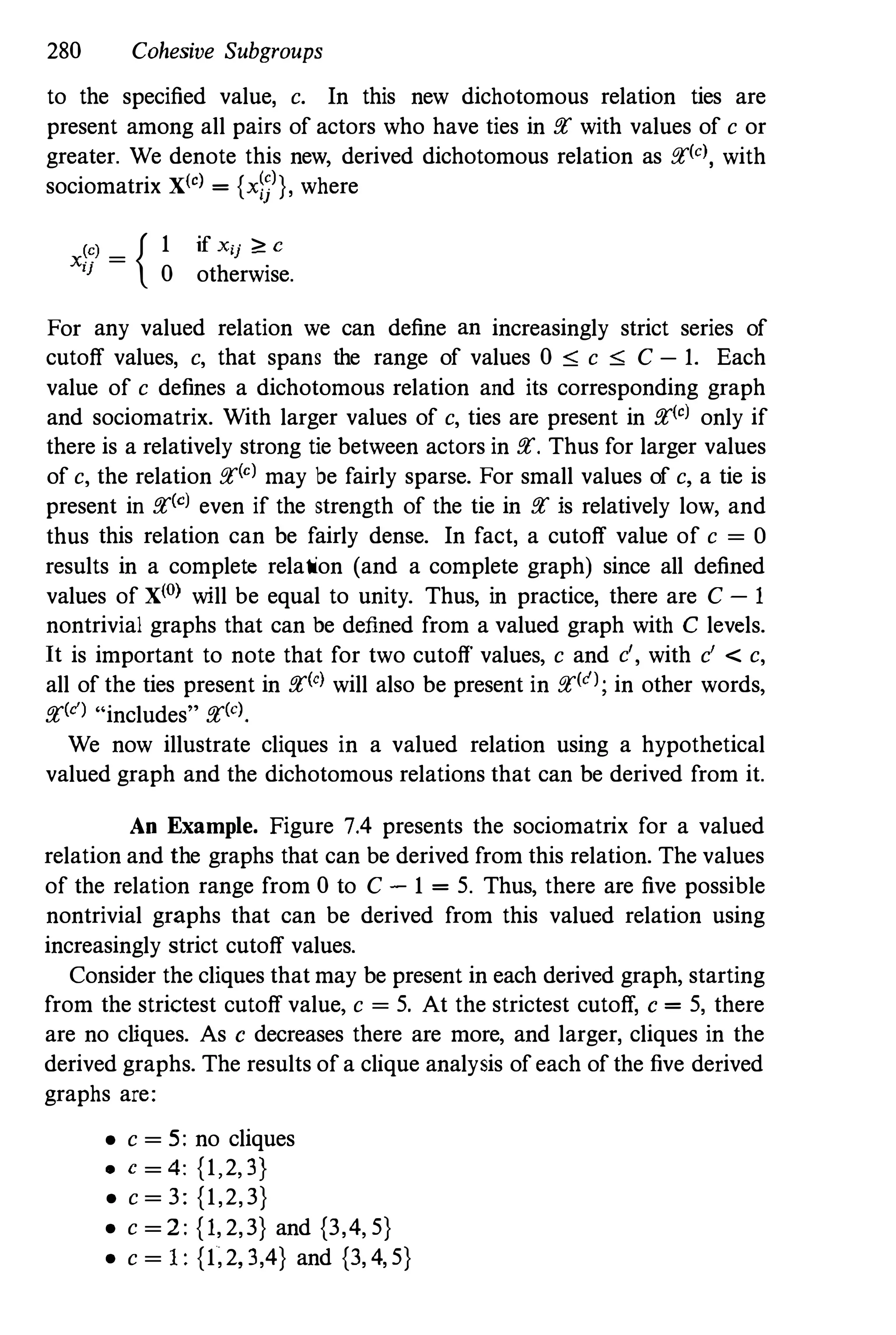
respect to degree. For this actor, C�(ng) = 0.400, an index considerably
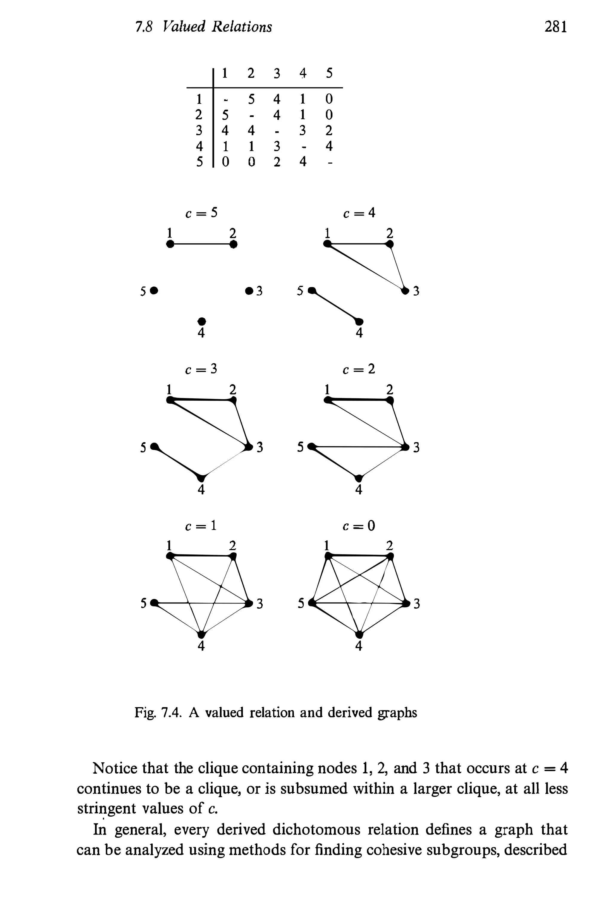
larger than the next most central actors (Guadagni and Strozzi families),
with Chin,) =Ch(n15) = 0.267. Six of the families have an index of
0.200; the remaining seven families have small indices. The group-level
degree centralization index is CD = 0.267, a rather small value, indicating
that the difference between the largest and smallest actor-level indices
is not very great. There is little variability. The average degree is
CD = 40/16 = 2.50, quite small, but not surprising given the nature
of the relation (marital ties, something not particularly common). We
also note that the variance of the degrees (not the standardized actor
5.2 Nondirectional Relations 183
Table 5.1. Centrality indicesfor Padgett's Florentine families (.Actor and
centralization indices calculated by dropping n12 = Pucci from the actor
set.)
With g = 16 actors With g = 15 actors
C1(nd C�(ni) C�(nil* C�(na· C�{nd· C;(nd*
Acciaiuoli 0.067 0.000 0.071 0.368 0.000 0.049
Albizzi 0.200 0.184 0.214 0.483 0.212 0.074
Barbadori 0.133 0.081 0.143 0.438 0.093 0.068
Bischeri 0.200 0.090 0.214 0.400 0.104 0.074
Castellani 0.200 0.048 0.214 0.389 0.055 0.070
Ginori 0.067 0.000 0.071 0.333 0.000 0.043
Guadagni 0.267 0.221 0.286 0.467 0.255 0.081
Lamberteschi 0.067 0.000 0.071 0.326 0.000 0.043
Medici 0.400 0.452 0.429 0.560 0.522 0.095
Pazzi 0.067 0.000 0.071 0.286 0.000 0.033
Peruzzi 0.200 0.019 0.214 0.368 0.022 0.069
Pucci 0.000 0.000 - - - -
Ridolfi 0.200 0.098 0.214 0.500 0.114 0.080
Salvati 0.133 0.124 0.143 0.389 0.143 0.050
Strozzi 0.267 0.089 0.286 0.438 0.103 0.070
Tornabuoni 0.200 0.079 0.214 0.483 0.092 0.080
Centralization 0.267 0.383 0.257 0.322 0.437 -
degree centrality indices) S� = 2.125, and the density of this relation
(which is the average standardized degree) is 0.167, indicating (as noted)
a relatively sparse sociomatrix. The density of this relation is quite a bit
less than that for the three hypothetical graphs in Figure 5.1, for instance.
5.2.2 Closeness Centrality
The second view of actor centrality is based on closeness or distance. The
measure focuses on how close an actor is to all the other actors in the
set of actors. The idea is that an actor is central if it can quickly interact
with all others. In the context of a communication relation, such actors
need not rely on other actors for the relaying of information, an idea
put forth by Bavelas (1950) and Leavitt (1951). As noted by Beauchamp
(1965), actors occupying central locations with respect to closeness can
be very productive in communicating information to the other actors. If
the actors in the set of actors are engaged in problem solving, and the
focus is on communication links, efficient solutions occur when one actor
184 Centrality and Prestige
has very short communication paths to the others. Thus, this closeness
view of centrality relies heavily on economic considerations.
Hakimi (1965) and Sabidussi (1966) quantified thls notion that cen­
tral actors are close, by stating that central nodes in a network have
"minimum steps" when relating to all other nodes; hence, the geodesics,
or shortest paths, linking the central nodes to the other nodes must be
as short as possible. With this explanation, researchers began equating
closeness with minimum distance. The idea is that centrality is inversely
related to distance. As a node grows farther apart in distance from other
nodes, its centrality will decrease, since there will be more lines in the
geodesics linking that node to the other nodes.
Examine the star network in Figure 5.1. The node at the center of thls
star is adjacent to all the other nodes, has the shortest possible paths to
all the other actors, and hence has maximum closeness. There is exactly
one actor who can reach all the other actors in a minimum number .of
steps. This actor need not rely on the other actors for its interactions,
since it is tied to all others.
Actor Closeness Centrality. Actor centrality measures reflecting
how close an actor is to the other actors in the network have been de­
veloped by Bavelas (1950), Harary (1959c), Beauchamp (1965), Sabidussi
(1966), Moxley and Moxley (1974), and Rogers (1974). As reviewed
by Freeman (1979), the simplest measure is that of Sabidussi (1966),
who proposed that actor closeness should be measured as a function of
geodesic distances. As mentioned above, as geodesics increase in length,
the centrality of the actors involved should decrease; consequently, dis­
tances, which measure the length of geodesics, will have to be weighted
inversely to arrive at Sabidllssi's index. Note how this type of centrality
depends not only on direct ties, but also on indirect ties, especially when
any two actors are not adjacent.
We let din"�nj) be the number of lines in the geodesic linking actors
i and j; that is, as defined in Chapter 4, d(., .) is a distance function.
The total distance that i is from all other actors is I:J�l din"� nj), where
the sum is taken over all j of i. Thus, Sabidussi's (1966) index of actor
closeness is
g �1
Cdn,) = [Ld(n,.n)]J=l
(5.7)
The subscript C is for "closeness." As one can see, the index is simply the
inverse of the sum of the distances from actor i to all the other actors.
5.2 Nondirectional Relations 185
At a maximum, the index equals (g- 1)-1, which arises when the actor is
adjacent to all other actors. At a minimum, the index attains the value of
o in its limit, which arises whenever one or more actors are not reachable
from the actor in question. A node is said to be reachable from another
node if there is a path linking the two nodes; otherwise, the nodes are
not reachable from each other. Thus, the index is only meaningful for a
connected graph.
To verify this assertion, suppose that the graph is disconnected -
specifically, let there be one isolated node, with degree O. The geodesics
from all the other nodes to this specific node (nk) are infinitely long
(d(n" nd = 00 for all i '" k), since the node is not reachable. Hence, the
distance sum for every actor is 00, and the actor closeness indices are all
O. This is a large drawback of this index.
As we have noted, the maximum value attained by this index depends
on g; thus, comparisons of values across networks of different sizes are
difficult. Beauchamp (1965) made the suggestion of standardizing the
indices so that the maximum value equals unity. To do this, we simply
multiply Cc(n,) by g - 1 :
g - 1
[ I:)�1 d(n" nj)j
= (g - I)Cc(n,). (5.8)
This standardized index ranges between 0 and 1, and can be viewed as
the inverse average distance between actor i and all the other actors. It
equals unity when the actor is adjacent to all other actors; that is, when
the actor is maximally close to all other actors.
Graph theorists have simplified this concept of centrality, and talked
about the center of a graph, using the graph-theoretic notion of distance
(see Chapter 4). Specifically, the Jordan center (see Jordan 1869) of a
graph is the subset of nodes that have the smallest maximum distance
to all other nodes. To find such a center, one can take a g x g matrix
of geodesic distances between pairs of nodes (where the entries are the
lengths of the shortest paths or geodesics between all pairs of nodes),
and then find the largest entry in each row. These distances (which are
sometimes called eccentricities) are the maximum distances from every
actor to their fellow actors. One then simply finds the smallest of these
maximum distances. All nodes that have this smallest maximum distance
are part of the center of the graph.
A related notion is the centroid of a graph (see Sylvester 1882), which
is based on the degrees of the nodes and which is most appropriate
186 Centrality and Prestige
for graphs that are trees. The idea is to consider all branches or paths
emanating from each node, and define the weight of each branch as the
number of lines in it. The weight of a node is the maximum weight of
any branch at the node. The centroid is thus the snbset of all nodes that
have the smallest weight.
All the graphs in Figure 5.1 are connected, so that all geodesic distances
are finite; therefore, the closeness indices can be calculated. For the
star graph, Ci;(n,) = 1.0, while the other actors all have indices equal
to 0.545. For the circle graph, the actor indices are all equal to 0.5.
For the line graph, the indices vary from Ci;(nll = 0.50 to a low of
CC(n6) = CC(n7) = 0.286.
We note that there are clever algorithms for finding the geodesics in
a graph, and then computing their lengths. We refer the reader to (for
example) Flament (1963), and Harary, Norman, and Cartwright (1965).
Such algorithms are standard in network computing programs such as
UCINET and SNAPS (see Appendix A).
Group Closeness Centralization. We now consider how to mea­
sure group centralization using actor closeness centralities. We first report
Freeman's (1979) index, which uses the general graph centralization in­
dex, (5.1), given above. We then will consider alternative group closeness
indices.
Freeman's general group closeness index is based on the standardized
actor closeness centralities, shown in equation (5.8). This index has
numerator
g
2)Cc(nO) - Cc(n,)],
i=l
where C�(nO) is the largest standardized actor closeness in the set of ac­
tors. Freeman shows that the maximum possible value for the numerator
is [(g - 2)(g - 1)]/(2g - 3), so that the index of group closeness is
Cc =
L:f-l[Cc(nO) - Cc(n,)]
[(g - 2)(g - 1)]/(2g - 3) ·
(5.9)
This index, as with the group degree centralization index, reaches its
maximum value of unity when one actor "chooses" all other g-1 actors
(that is, has geodesics of length 1 to all the other actors), and the other
actors have geodesics of length 2 to the remaining (g - 2) actors. This is
exactly the situation realized by a star graph. The proof of this fact is
rather complicated, and must be done by induction. We refer the reader
5.2 Nondirectional Relations 187
to Freeman (1979). The index can attain its minimum value of 0 when
the lengths of geodesics are all equal, for example in a complete graph
or in a circle graph. For the line graph of Figure 5.1, the index equals
0.277, a relatively small value.
Bolland (1988) proposes a measure (for both actors and groups) that
utilizes both degree and doseness of actors. His "continuing flow"
centrality index is based on the number of paths (of any length) that
originate with each actor. Thns, the measure considers all paths, those of
length 1 (that are the focus of CD) and those indirect (whose distances
are reflected in the magnitude of Cc). We discuss this measure in more
detail at the end of this chapter.
There are other group�level closeness indices. We filay simply sum­
marize the set of g actor-level closeness centralities {CC(ni)} by a single
statistic, reflecting the tendency toward closeness manifested by all the
actors in the set of actors. Such a statistic, to be an effective index, should
reach its extremes in the cases of the circle graph (equal distances), and
the star graph (one minimally distant actor).
We recommend that one calculate the variance of the standardized
actor closeness indices,
s� = [t(Cc(ni)-cd]/g, (5.10)
which summarizes the heterogeneity among the {CC(ni)}. We note that
average normed closeness, Cc = 2: C(,(ni)/g, is simply the mean of
the actor-level closeness centralities. The variance attains its minimum
value of 0 in a network with equal actor indices (in this case, equal
distances between all nodes). Such a network need not be complete
(have maximal degree). This index grows as the network becomes less
homogeneous (with respect to distances), and thus more centralized. The
average normed closeness, Ce, together with S1:, provide simple summary
statistics for the entire set of actor closeness indices.
The Example Again. Consider again Padgett's network data, dis­
cussed earlier. Actor n12 = Pucci (as can be seen from the actor degree
centrality value of Cn(n12) = 0) is an isolate. Consequently, the distances
to this actor from all other actors are infinite, and thus, family Pucci is
not reachable and the graph is not connected. Actor closeness centrality
indices are then also infinite, and cannot be calculated.
Thus, we dropped family Pucci from the set of actors, giving us a
smaller network of g -1 = 15 families, but now we have (for the purpose
188 Centrality and Prestige
of demonstrating the calculations of closeness centralities) a connected
graph. The actor centralities and centralization indices calculated for this
smaller network are shown in Table 5.1 and are indexed with asterisks
to distinguish them from indices calculated for the full set of actors. The
actor closeness centralities are shown in Column 4, while the actor degree
centralities for the smaller set of actors (sans family Pucci) are shown
in Column 3. Once again family Medici is the most central actor, but
several families are almost as central: Albizzi, Guadagni, Ridolfi, and
Tornabuoni.
Note that family Strozzi, which had a rather large actor degree central­
ity index, has a relatively small actor closeness centrality index. Strozzi
has apparently married into a moderately large number of other families,
but is not particularly close to the other families; that is, there are many
"steps" in the marital linkages from Strozzi to the others.
The closeness indices are much larger than the degree indices, and
none of the families have small values. Families Acciaiuoli, Ginori,
Lamberteschi, and Pazzi are still the least central. These indices also
vary less than the degree indices (from 0.326 to 0.560, as opposed to
0.071 to 0.429 for degree centralities), indicating a much more uniform
spread of closenesses. The closeness centralization index is Cc = 0.322,
calculated for the smaller network, and the average closeness centrality
and variance are Cc = 0.415 and s1: = 0.0056. This is a small variance,
indicating once again the small range of the actor closeness centralities.
5.2.3 Betweenness Centrality
Interactions between two nonadjacent actors might depend on the other
actors in the set of actors, especially the actors who lie on the paths be­
tween the two. These "other actors" potentially might have some control
over the interactions between the two nonadjacent actors. Consider now
whether a particular actor might be able to control interactions between
pairs of other actors in the network. For example, if the geodesic between
actors n, and n3 is n,nln4n3 - that is, the shortest path between these
actors has to go "through" two other actors, nl and n4 - then we could
say that the two actors contained in the geodesic might have control
over the interaction between n2 and n3. Glance again at our star network
in Figure 5.1, and note that the most central actor lies on all fifteen
geodesics linking the other six actors. This "actor in the middle," the one
between the others, has some control over paths in the graph. A look at
the line network in Figure 5.1 shows that the actors in the middle of this
5.2 Nondirectional Relations 189
graph might have control over some of the paths, while those at the edge
might not. Or, one could state that the "actors in the middle" have more
"interpersonal influence" on the others (see Freeman 1979, or Friedkin
1991).
The important idea here is that an actor is central if it lies between
other actors on their geodesics, implying that to have a large "between­
ness" centrality, the actor must be between many of the actors via their
geodesics.
Several early centrality researchers recognized the strategic importance
of locations on geodesics. Both Bavelas (1948) and Shaw (1954) sug­
gested that actors located on many geodesics are indeed central to the
network, while Shimbel (1953) and Cohn and Marriott (1958) noted that
such central actors play important roles in the network. None of these
researchers, however, were able to quantify this notion of betweenness.
It took roughly twenty years, however, until Anthonisse (1971), and later
Freeman (1977) and Pitts (1979), suggested that the the locations of
actors on geodesics be examined.
Actor Betweenness Centrality. Let us simply quote from Shimbel
(1953), reiterated by Pitts (1979), who stated the importance of geodesics
and the actors they contain for measuring betweenness and network
control:
Suppose that in order for [actor] i to contact [actor] j, [actor] k must
be used as an intermediate station. [Actor] k in such a network has
a certain "responsibility" to [actors] i and j. If we count all of the
minimum paths which pass through [actor] k, then we have a measure
of the "stress" which [actor] k must undergo during the activity of the
network. (page 507)
Here, actors who have sufficient stress also possess betweenness, accord­
ing to this rather political view of network flows.
Specifically, one shonld first count the number of geodesics linking
actors j and k (all these geodesics will be of the same length, d(nj,nd),
and then determine how many of these geodesics contain actor i, for all
distinct indices i,j,k. Shimbel goes on to state that
A vector giving this [count of minimum paths] for each [actor] of the
network would give us a good idea of the stress conditions throughout
the system. (page 507; emphasis is ours)
Shaw (1954) was the first to recognize that this stress was also be­
tweenness, noting that, in the case of a communication relation where
190 Centrality and Prestige
actors could not form new lines, central actors could refuse to pass along
messages. Anthonisse (1971) and Freeman (1977) first quantified this
idea.
We want to consider the probability that a "communication," or simply
a path, from actor j to actor k takes a particular route. We assume that
lines have equal weight, and that communications will travel along the
shortest route (regardless of the actors along the route). Since we are
just considering shortest paths, we assume that such a communication
follows one of the geodesics. When there is more than one geodesic
between j and k, all geodesics are equally likely to be used. Freeman
estimates this probability as follows: Let gjk be the number of geodesics
linking the two actors. Then, if all these geodesics are equally likely to be
chosen for the path, the probability of the communication using any one
of them is simply l/gjk. We also consider the probability that a distinct
actor, i, is "involved" in the communication between the two actors. We
let gjk(n,) be the number of geodesics linking the two act'lTS that contain
actor i. Freeman then estimates this probability by gjk(n,)/gj" making
the critical assumption that geodesics are equally likely to be chosen for
this path. (We comment on this assumption later in the chapter.)
The actor betweenness index for n, is simply the sum of these estimated
probabilities over all pairs of actors not including the ith actor:
CB(n;) = :L:.>jk(n,)/gjk (5.11)
j<k
for i distinct from j and k. So, this index, which counts how "between"
each of the actors is, is a sum of probabilities. It has a minimum of
zero, attained when n, falls on no geodesics. Its maximum is clearly
(g- 1)(g-2)/2, which is the number of pairs of actors not including n,.
The index reaches the maximum when the ith actor falls on all geodesics.
Since the index's values depend on g, we standardize it just like the other .
actor centrality indices:
C�(ni) = CB(n,)/[(g- 1)(g - 2)/2]. (5.12)
Standardized in this way, it now takes on values between 0 and 1, and
can easily be compared to the other actor indices, as well as across
networks and relations. Unlike the closeness indices, these betweenness
indices {C�(n;)} can be computed even if the graph is not connected. This
is certainly an advantage. As with our other actor indices, algorithms for
first finding the geodesics in a graph, and then counting how many of
5.2 Nondirectional Relations 191
them contain each of the actors, are available, and are implemented in
network computer programs such as UCINET.
The quantities summed on the right-hand side of equation (5.11) are
discussed in more detail in Freeman (1980a). Specifically, if we sum
the gjk(n,)/gjk estimated probabilities over k, we obtain measures of the
pair-dependency of actor j on actor i. These values, which can also
be viewed as indices of how much "gatekeeping" n, does for nj, are
crucial components of both the {CB(nj)) and the {Cc(nj)). Gatekeeping
of one actor for another is simply the act of being on geodesics from
the latter actor to all other actors, regardless of where the geodesics are
going. Actors on whom others are "locally dependent" are central in
the network. One can measure the level of gatekeeping for every pair
of actors in the network, focusing on how much gatekeeping the second
actor does for the first.
Returning again to the graphs of Figure 5.1, we find that for the
star graph, C�(n,) = 1.0, while C�(n2) = . . . = C�(n7) = O. This is an
idealized situation, since only actor 1 lies on any of the geodesics. The
actor betweenness indices in the circle graph are all equal to 0.2, and
for the line graph, vary from C],(nl) = 0.6 to C�(n6) = C�(m) = O.
In this last graph, actors n, and n3 are almost as central as n1. since
C�(n2) = C�(n3) = 0.533.
Group Betweenness Centralization. Group centralization indicies
based on betweenness allow a researcher to compare different networks
with respect to the heterogeneity of the betweenness of the members of
the networks. We first report Freeman's (1979) index for quantifying the
overall level of betweenness in the set of actors, which summarizes the
actor betweenness indices given in equation (5.11).
Freeman's group betweenness centralization index has numerator
I:;�l[CB(n')- CB(n,)], where CB(n') is the largest realized actor between­
ness index for the set of actors. The reason for using the nonstandardized
indices rather than the standardized ones (see equation (5.12)) will fol­
low. Freeman shows that the maximum possible value for this Sum is
(g - 1)'(g - 2)/2, so that the index of group betweenness is
CB =
2I:f-l[CB(n')- CB(n,)]
[(g - 1)2(g . 2)]
(5.13)
Freeman (1979) shows that this simplifies to the index given in Freeman
(1977) :
192 Centrality and Prestige
C
_ 2:f-1[C�(n')- C�(ni)l .B -
(g - l)
, (5.14)
that is, the calculation can also be made equivalently with the standard­
ized indices. Freeman (1977) also demonstrates that the index reaches its
maximum value (unity) for the star graph. Its minimum value (0) occurs
when all actors have exactly the same actor betweenness index - that
is, in a network in which all actors are equal in betweenness. The line
graph of Figure 5.1 has CB = 0.311.
There are additional group-level betweenness indices, for example the
variance of the actor-level betweenness indices. Such centralization in­
dices provide additional summaries of the heterogeneity or variability of
betweenness in the entire set of actors.
The Example, Once Again. Actor betweenness centralities are
given for Padgett's Florentine families and the marriage relation in Ta­
ble 5.1, Columns 2 and 5. The second column gives the betweenness
centralities calculated for the network consisting of all actors, and the
fifth column, for the network without the Pucci family. Note how many
actors have 0 indices - families Acciaiuoli, Ginori, Lamberteschi, Pazzi,
and of course Pucci - the same actors that had the smallest actor close­
ness centrality indices. The betweenness indices allow the Medici family,
and, to a lesser extent, the Guadagni family, to stand out, just as with
the actor degree centralities.
Clearly, families Medici and (perhaps) Guadagni are the most central
families in this set of actors on this marital relation. The betweenness
centralization index is CB = 0.437, larger than the other centralization
indices, reflecting the fact that the Medici family is much more central
than any of the other families.
Note how these betweenness indices compare to the other two actor
centrality indices. Some actors with moderately large closeness and
degree scores have small betweenness indices - families Barbadori and '
especially Tornabuoni. Family Strozzi, which has a large degree index; has
a small betweenness index. Such differences indicate that the betweenness
indices can be quite different measures of actor centrality than degree­
and closeness-based indices.
5.2.4 ®Injormation Centrality
Of all these indices, Freeman's centrality measure based on betweenness
of actors on geodesics has found the most use, because of its general-
5.2 Nondirectional Relations 193
ity. But. this index assumes that all geodesics are equally likely when
estimating the critical probability that an actor falls on a particular
geodesic. That is, if there are gij geodesics between actors i and j, then
the probability that a particular geodesic is "chosen" for the "flow of
information" between these two actors is simply l/gij. While this is a
justifiable assumption for some purposes, it may not be appropriate here.
Suppose we focus on the actors "contained" in these geodesics. Free­
man ignores the fact that if some actors on the geodesics have large
degrees, then the geodesics containing these expansive actors are more
likely to be used as shortest paths than other geodesics. That is, if an
actor has a degree of, say, 10, and this actor is on a geodesic, then
this actor is more likely than actors with smaller degrees to be on other
geodesics, simply because of its expansiveness. Freeman's assumption is
reasonable only if all actors have equal degrees. For such regular graphs,
it is not unreasonable to assume that all geodesics between a pair of
nodes are equally likely to be "used" for a path. Relaxing this assump­
tion is difficult, and requires a more sophisticated statistical model that
allows for unequal probabilities.
A second, more important generalization can also be considered. Free­
man, in considering betweenness counts, focuses only on geodesics. That
is, paths with distances greater than the minimum path length attained
by the geodesics are ignored. Substantively, this might not be realistic.
For example, if we consider communication relations, there may be good
reasons for actors to choose paths for their communications that are
longer than the geodesics. We quote:
It is quite possible that information will take a more circuitous route
either by random communication or [by being] channeled through many
intermediaries in order to "hide" or "shield" information. (Stephenson
and Zelen 1989, page 3)
So, it may make sense to generalize the notion of betweenness centrality
so all paths between actors, with weights depending on their lengths, are
considered when calcnlating betweenness counts.
The index of centrality developed by Stephenson and Zelen (1989)
does exactly this. One considers the combined path from one actor to
another, by taking all paths, including the geodesics, and assigning them
weights. A weighted function of this combined path is then calcnlated,
using as weights the inverses of the lengths of the paths being combined.
The weights assigned to the paths making up the combined path are
determined so that the "information" in the combined path is maximized.
194 Centrality and Prestige
Geodesics are usually given weights of unity, while paths with lengths
longer than the geodesic length receive smaller weights based on the
i�formation that they contain. The information of a path is defined quite
simply as the inverse of its length.
Mackenzie (1966b) was the first to propose the use of information
theory for the study of centrality, particularly in commnication networks.
He defined a "Total Participation Index" for actors in a network, but his
rather mathematical presentation has prevented wider adoption of the
idea. Bolland's (1988) index of continuing flow also considers all paths
originating with each actor, but does not consider betweenness counts.
The concept of information is quite old, and has a rich tradition in
statistics (Shannon and Weaver 1949; Khinchin 1957; Kullback 1959;
Gokhale and Kullback 19n; see also Coleman 1964; Theil 1967; and
Allison 1978, for applications in economics and sociology). It is used
extensively in estimation theory and categorical data analysis. Informa­
tion is usually defined as the inverse of the variance of an estimator. If
an estimator has a small variance, it has large information, and thus is
considered "good." The opposite is also true: poor estimators with large
variances have little information. We can apply this approach to central­
ity by extending betweenness on geodesics to all possible paths, weighting
according to the information that these paths contain. The betweenness
counts are then generalized to reflect the information contained in all
paths.
Stephenson and Zelen (1989) give a nice discussion of the use of
information in statistical estimation as applied to the paths between
nodes in a graph. In brief, the length of any path is directly related to
the variance of transmitting a signal from one node to another; thus, the
information contained in this path is the reciprocal of this variance. Thus,
any path (and hence, each and every combined path) has an "information
content." Lastly, the information of a node is the harmonic average of
the information for the combined paths from the node to all other nodes.
Actor Information Centrality. This version of centrality focuses
on the information contained in all paths originating with a specific actor.
The information of an actor averages the information in these paths,
which, in turn, is inversely related to the variance in the transmission of
a signal from one actor to another.
To calculate information centrality indices, Stephenson and Zelen rec­
ognized that the information contained in an incidence matrix (see Chap­
ter 4), which codes the nodes and the links between them, is exactly the
5.2 Nondirectional Relations 195
same as the information contained in the data vector and incidence ma­
trix for an incomplete block design with two treatments per block (see
Cochran and Cox 1957). This exact equality allowed Stephenson and
Zelen to adopt a statistical model, common in the statistical design of
experiments (see St. John and Draper 1975; Box, Hunter, and Hunter
1978; Silvey 1981), designed for such incomplete block designs. The
model focuses on all the "signals" flowing between all pairs of nodes
("r pairs of rows of the incidence matrix). One estimates the strengths
of these signals, and calculates their variances. If Vjk is the variance of
the estimate of the signal for the path linking nodes nj and n" then the
information associated with this path is simply I/Vjk. The information
for an actor is a function of all the information for paths flowing out
from the actor. The chosen function is the harmonic average. We refer
the reader to the appendix of Stephenson and Zelen (1989) for more
mathematical details.
To apply this idea to graphs, the actor information indices are functions
of a simple g x g matrix. We give the most general formulation of
the index, which assumes that the relation is nondirectional, but not
necessarily dichotomous. A crucial component ofthe formula is the sum
of the strengths or values for the lines incident with a node. This sum is
simply a row total (or column total) of the sociomatrix. The sum is the
degree of a node when the measured relation is dichotomous, or the sum
of the strengths ofall ties incident to a node when the relation is valued.
The calculation begins as follows. One first creates a g x g matrix A,
which has diagonal elements
a" = 1 + sum of values for all lines incident to n,
and off-diagonal elements
aij =
{ I
I - Xij
if nodes n, and nj are not adjacent
if nodes n, and nj are adjacent.
(5.15)
(5.16)
As usual, xij is the value of the tie between actors i and j, so that
the elements of A are easily calculated from the sociomatrix. One next
calculates the inverse of A: C = A-I, which has elements {cij}.
We should note that not every A matrix can be inverted. In fact, if the
sociomatrix has one (or more) rows (and hence columns) full of zeros,
the corresponding C is not defined. In this instance, actor information
centralities cannot be computed. We recommend that the actors who are
isolates be dropped from the set of actors, and indices calculated just for
the non-isolates.
196 Centrality and Prestige
To get the information indices, one needs two intermediate quantities.
These are sums of elements of C: T = 2:f�1 eii and R = 2:5�1 cij' T is
simply the trace or the sum of the diagonal entries of the matrix, while
R is any one of the row sums (all the row sums are equal). With these
two quantities, and the elements of C, one lastly calculates
1
Cl(n;) = -�=-,,--�
C" + (T - 2R)/g
as the information centrality index for actor i.
(5.17)
This index measures how much information is contained in the paths
that originate (and end) at a specific actor. The index has a minimum
value of 0, but no maximum value; indeed, if T = 2R, and Cji = 0, the
index would equal 00. Stephenson and Zelen (1989) recommend that One
use relative information indices, obtained by dividing each index Cl(ni)
by the total of all indices:
, Cl(n;)
Cl(ni) =
2:i Cl (ni) ' (5.18)
The relative information indices, {C;(niJ}, are bounded by 0 and 1, and
sum to unity. These indices can be interpreted as the proportion of total
"information" flow in a graph controlled by an individual actor. The
constraint that the indices sum to unity is unique to this index, and
makes comparisons with the other actor-level centrality indices difficult.
Necessary calculations are not complicated, and involve manipulations of
the sociomatrix, and then a single matrix inversion. One can "program"
them with SAS PROC IML or GAUSS.
Return once again to the graphs of Figure 5.1. We find that for
the star graph, C;(nIl = 0.2340, while C;(n2) = . . . = C�(n7) = 0.1277.
Notice that even though only node nl lies on any of the geodesics, the
information centralities for the other six nodes are not zero. The actor
information indices in the circle graph are all equal to 0.1429, and for the
line graph, vary from C;(nl) = 0.1822 to q(n,) = C�(n7) = 0.1041. In
this last graph, nodes n2 and n3 are almost as central as nl, since C�(n2) =
C�(n3) = 0.1682. Remember that the actor information centralities are
normed differently from the other actor centralities � they must sum to
unity, so that if one actor has a large index, the other actors must have
smaller indices.
Use of this information index has been limited. Stephenson (1989)
and Stephenson and Zelen (1989) apply this methodology to networks of
baboons, while Stephenson (1989) and Frey (1989) use this index (and
5.2 Nondirectional Relations 197
others) to study a network of forty AIDS patients, linked by sexual
contact (Auerbach, Darrow, Jaffe, and Curran 1984; Klovdahl 1985; see
also Laumann, Gagnon, Michaels, Michael, and Coleman 1989; Morris
1989, 1990). Marsden (1990b) has used information indices in a study
of the effect of random sampling on estimation of the parameters of the
network effects or social process model (see Erbring and Young 1979;
Doreian 1981; Friedkin 1986, 1990; Marsden 1990a; and Burt 1987).
Group Information Centralization. The summary group-level in­
formation index proposed by Stephenson and Zelen is simply the average
information across actors:
(5.19)
This index has limits that depend on g, unfortunately, and so is difficult to
compare across networks. As we have mentioned throughout this chapter,
averages are not centralization indices. A real group-level information
centralization index is the variance of the actor information indices :
si = [t(c;(ni) - Cd]/g. (5.20)
One could also apply Freeman's (1979) general index (5.1) to informa­
tion indices, although (to our knowledge) no one has calculated the
denominator (the maximum possible sum of differences between the ob­
served indices and the largest attained index) for a Freeman information
centralization index.
For the graphs of Figure 5.1, the variances are 0.001614, 0.000986, and
0.0, for the star, line, and circle graphs, respectively. Thus, the star graph
is most heterogeneous, and the circle, the least.
As mentioned, this information actor-level index of centrality is the
only index (that we are aware of) that can be applied to valued relations.
Further, as we have discussed, it generalizes Freeman's widely used
index of betweenness, since it considers all paths, not just geodesics.
We comment further on the differences among all the indices discussed
here at the end of the chapter. Further research and application should
demonstrate the usefulness of the actor information centrality index
(5.18).
Last Look at Padgett's Florentine Families. As we have noted,
family Pucci is not married to any other families; it is an isolate, and
consequently, the actor information centralities cannot be calculated
198 Centrality and Prestige
because the C matrix cannot be inverted. Thus, we dropped this actor
from the set of actors, and calculated actor information centralities for
the other fifteen actors. These indices are shown in Column 6 of Table 5.1.
It is difficult to compare these indices to the others, since only the
information centralities are constrained to sum to unity. They must be
between 0 and 1, just like all the other types of centrality, but are forced
to be smaller in magnitude because of this constraint.
The Medici family is still the most central family, although the
Guadagni, Tornabuoni, and Ridolfi families have indices not much
smaller than that for Medici. These four families consistently have
the largest actor centrality indices. The Pazz� Ginori, Lambertesch� and
Acciaiuoli families are the least central families ; in fact, the ordering of
the actors with respect to information centrality is almost identical to
that for betweenness centrality, The main difference between the two
sets of centralities is the range of values - the range is much smaller
for information. The variance of the actor information centralities is
Sf = 0.000297, quite small, reflecting the small range of the values due
to the unity summation constraint.
We now turn to indices that can be applied to social network data
consisting of directional relations.
5.3 Directional Relations
In the previous section, we discussed nondirectional relations, and intro­
duced four actur-Ievel indices for centrality (and associated centralization
indices). These indices are:
(i) Degree - equation (5.3)
(ii) Closeness - equation (5.8)
(iii) Betweenness - equation (5.12)
(iv) Information - equation (5.18)
We now discuss how these, and other kinds ofindices (specifically, those
designed to measure prestige), can be calculated for directional relations.
Suppose that we have a single set of actors, and a single, dichotomous
directional relation. With such data, we can distinguish between "choices
made" and "choices received." An example of such data that we will
be analyzing in this section can be found in Chapter 2; specifically, the
countries trade network data which show import and export of basic
manufactured goods among a collection of g=24 countries. These data
are discussed in some detail in Chapter 2, and will be examined at
5.3 Directional Relations 199
length in Chapters 9-12. Clearly for these data. imports are substantively
different from exports, and it is interesting to study which actors are
important importers and which are significant exporters. To identify
these important actors on this relation, we will examine both aspects of
prominence: centrality and prestige.
As mentioned at the beginning of the chapter, centrality indices for
directional relations generally focus on choices made, while prestige
indices generally examine choices received, both direct and indirect. We
will discuss how to calculate centrality indices for directional relations
here, but the emphasis in this section will be prestige, and in particular,
three types of prestige indices.
We first discuss how the four centrality indices, degree, closeness,
betweenness, and information, can be extended to directional relations.
For this extension, we examine actors from the perspective of the choices
or nominations. that are made. Two of the centrality indices are easily
applied to directional relations (degree and closeness indices), while the
other two (betweenness and information), because of their reliance on
nondirected paths and geodesics, are not.
One can also examine the choices received by actors. This allows us to
study which actors in the set of actors are prestigious. We will present
and discuss three types of prestige indices.
5.3.1 Centrality
To extend to directional relations the centrality indices based on degree,
closeness, betweenness, and information, and the group-level indices
which aggregate the actor-level indices (equations (5.5), (5.9), (5.13),
(5.19)), we must consider how each is computed and how the network
properties that are crucial for each are defined for directional relations.
Degree. An actor index for degree centrality can easily be cal­
culated for directional relations. Such indices are meaningful if no
restrictions, as in a. fixed choice design, are placed on the choices made
by the actors. Since centrality indices focus on the choices made, we
take the outdegree of each actor, rather than the degree (which we used
for nondirectional relations) : eben,) = x,+/(g -
1). A group-level index
of degree centralization can be calculated as suggested in equation (5.4).
The denominator of this index when the measured relation is directional
can be calculated to be (g - lf. These actor and group-level indices have
exactly the same properties as degree indices for nondirectional relations.
200 Centrality and Prestige
Closeness. An actor index for closeness centrality can also be
calculated for directional relations. Specifically, we define the distances
between any two actors, as discussed in Chapter 4, as the length of the
geodesic(s) from n; to nj. With a directed graph, the geodesic(s) from n;
to nj may not be tbe same as the one(s) from nj to n;, so that d(n;, nj),
the length of the geodesic(s), may not equal d(nj, n;). These {d(n;,nj)} are
elements of a g X g distance matrix.
Actor-level centrality indices for closeness are calculated by taking the
sum ofrow i of the distance matrix to obtain the total distance n; is from
all the other actors, and then dividing by g - 1 (the minimum possible
total distance). The reciprocal of this ratio gives us an actor-level index
for closeness. The formula is exactly the same as for nondirectional rela­
tions. Specifically, the actor-level closeness centrality index for directional
relations is
(5.21)
This index has exactly the same properties as discussed following equation
(5.8). A group-level closeness index based on Freeman's general formula
(5.1) can be obtained using the standardized indices ; however, to Our
knowledge, no one has calculated the denominator of this index when
the measured relation is directional.
One problem with this actor-level centrality index based on closeness
is that it is not defined unless the digraph is strongly connected (that is,
if there is a directed path from i to j, for all actors i and j); otherwise,
some of the {d(n;,nj)} will be co, and equation (5.21) will be undefined.
The same problem arises with graphs based on nondirectional relations,
as discussed earlier. One remedy to this problem is to consider only those
actors that i can reach, ignoring those that are unreachable from i.
This simple index, C�(n;), can be generalized by considering the in­
fluence range of n; as the set of actors who are reachable from n;. This
set contains all actors who are reachable from i in a finite number of
steps. This notion is common to graph theory, and is related to an idea
first used by Lin (1976) to describe the set of actors reachable to n; (see
below). We define J; as the number of actors in the influence range of
actor i. This count J; equals the number of actors who are reachable from
n;. Note that this idea can also be applied to nondirectional relations.
An "improved" actor-level centrality closeness index considers how
proximate n; is to the actors in its influence range. We define closeness
5.3 Directional Relations 201
now byjust focusing on distances from actor i to the actors in its influence
range. We consider the average distance these actors are from n,. This
average distance, Ld(n" nj)/J" where the sum is taken over all actors j
in the influence range of actor i, is a refined measure of closeness. Note
that this sum ignores actors who are not reachable from n" so that unlike
the first closeness centrality measures, it is defined even if the graph is
not strongly connected. We can define
• J;/(g - 1)
Cdn,) =
L d(n" nj}/J,' (5.22)
where the summation again is just over those actors in the influence
range of nj.
One can see that this index is a ratio of the fraction of the actors in
the group who are reachable (J,/(g - 1)), to the average distance that
these actors are from the actor (L d(n" nj)/J,). This index is quite similar
to an index for prestige that we discuss in the next section.
Other. The other two centrality indices for nondirectional rela­
tions, based on betweenness and information, were derived using theory
and algorithms designed specifically for nondirectional relations. Gould
(1987) has extended the betweenness index to directional relations, by
considering geodesics between any two actors. Gould shows that the al­
gorithm to find actor betweenness indices for nondirectional relations can
be applied to directional relations, since the basic algorithm automatically
uses ordered (rather than unordered) pairs of actors.
The {CB(n,)} indices defined in equation (5.11) are thus calculated
correctly for both directional and nondirectional relations; however, the
{C�(n,)} indices defined in equation (5.12) must be multiplied by 2. The
maximum value for the index is (g - 1)(g - 2), so that these standardized
scores must be multiplied by a factor of two to be correct (since the
maximum for nondirectional relations is (g - 1)(g - 2)/2). We note that
Gould's (1987) extension is based on the assumption that a directional
relation can be turned into a nondirectional relation by coding all mutual
dyads as lines and ignoring asymmetric dyads. Thus, there is a line in the
derived undirected graph between two actors if and only if both actors
choose each other in the original digraph.
For an information index, we could consider directed geodesics and
longer directed paths between actors. All these paths will be directed,
given the nature of the data. However, we do not know how to gen-
202 Centrality and Prestige
eralize Stephenson and Zelen's (1989) theory for information indices to
directional relations.
Thus, we recommend the use of just two centrality indices, C�(n,),
and C�(n,) or Cc(n;), for directed graphs. In our later discussions of
the countries trade network data, we calculate not only actor prestige
indices, but also these two actor centrality indices. Since choices received
are usually more interesting than those made, neither of these centrality
indices is as useful as the measures of prestige that we discuss below. If
the relation allows one to distinguish between choices made and choices
received, then the latter, along with prestige indices calculated from them,
can give important insights into social structure, as we will demonstrate
with our example.
5.3.2 Prestige
With directional relations, choices received are quite interesting to a
network analyst. Thus, measures of centrality may not be of as much
concern as measures of prestige. We now discuss several prestige mea­
sures, which we will illustrate on the countries trade network data. We
recommend that both centrality and prestige measures be computed for
directional relations, since they do attempt to measure different structural
properties.
There has been little research on group-level prestige indices. However,
such measures would certainly be welcome and interesting, since they
could quantify prestige heterogeneity (and possibly hierarchization or
network stratification).
We also note that there has been little work done on applications of
prestige measures to actual digraphs. For example, it is not known which
digraphs have maximal group-level prestige indices. More research on
such important issues is clearly needed.
Degree Prestige. The simplest actor-level measure of prestige is
the indegree of each actor, which we denoted by d1(n;) in Chapter 4. The
idea is that actors who are prestigious tend to receive many nominations
or choices (see Alexander 1963). So, we define
(5.23)
As with the comparable indices based on outdegrees, equation (5.23) is
dependent upon the group size g; thus, the standardization
5.3 Directional Relations
P' (
.
)
_ X+i
D nj -
g - l
203
(5.24)
gives us the proportion of actors who choose actor i, which is sometimes
called a "relative indegree." The larger this index is, the more prestigious
is the actor. Maximum prestige occurs when P�(ni) = 1 ; that is, when
actor i is chosen by all other actors. This index is quite simple to com­
pute, and is usually provided as output from network analysis computer
packages, such as UCINET.
Proximity Prestige. This simple index, P�(ni)' counts only actors
who are adjacent to actor i. One can generalize this index by defining the
irifluence domain of actor I as the set of actors who are both directly and
indirectly linked to actor j. Such actors are reachable to i, or alternatively,
are those from whom i is reachable. Reachability is discussed in Chapter
4. Thus, the influence domain consists of all actors whose entries in the
ith column of the distance matrix or the reachability matrix are finite.
This notion was first used by Lin (1976). We define Ii as the number of
actors in the influence domain of actor i. This count Ij equals the number
of actors who can reach actor i. We use the idea of an influence domain
in the next prestige index.
A second actor-level index of prestige considers how proximate ni is
to the actors in its influence domain. We define proximity as closeness
that focuses on distances to rather than from each actor. In other words,
what matters now is how close all the actors are to ni. Since the relation
is directional, such closeness will no doubt differ from the closeness that
ni is to the other actors. As stressed in Chapter 4, with digraphs, distance
to a node can be quite different from distancefrom.
We consider the average distance these actors are to ni. This average
distance, ,£d(nj, ni)/l;, where the sum is taken over all actors j in the
influence domain of actor i. is a crude measure of proximity. Note that
it ignores actors who cannot reach ni, so that unlike our closeness and
information centrality measures, it is defined even if the network is not
connected (when some aclors are not reachable from other actors). This
index depends on the size of the group, and is difficult to compare across
networks.
But, we can look at the ratio ofthe proportion of actors who can reach
i to the average distance these actors are from i. Thus, a better measure
of proximity takes the average distance, standardizes it, and then takes
reciprocals. From a suggestion by Lin (1976), we define
204 Centrality and Prestige
I,/(g - 1)
Pp(n,) =
�d(nj,n,)/I,'
(5.25)
where the summation again is just over those actors in the influence
domain of n,. One can easily see that this index is a ratio of the fraction
of the actors in the set of actors who can reach an actor (I,j(g - 1)) to
the average distance that these actors arc to the actor (�d(nj, n,)/I,). As
actors who can reach i become closer, on average, then the ratio becomes
larger.
This ratio index, based on the average distance actors in an influence
domain are to i, has the same properties as the centrality index for actor
closeness (see equation (5.7)). The index weights prestige according to
closeness or proximity. Note that if all actors are adjacent to ni, then
all the d(nj, n,) = 1, I, = g - 1, and the average standardized distance
is simply 1/(g - 1). This gives Pp(n,) = 1, the maximum value of the
prestige actor proximity index. If an actor is unreachable, then I, = 0,
and Pp(n,) = O. Thus, the limits of this index are 0 and 1, and the
magnitude of the index reflects how proximate an actor is from the set of
actors as a whole. Similar indices were proposed by Mackenzie (1966a)
and Arney (1973).
One could easily take the variance of the {Pp(n,J} to obtain a group­
level prestige index based on proximity. In addition, the average of
the actor-level indices can be used to summarize the set of actors as a
whole. The average is proportional to the average of the reciprocals of
the average distances to the actors. These two group-level indices are
and
g - 2sf,
=
� (Pp(n,) - Pp)
i=l
g
(5.26)
(5.27)
The average will be between 0 and 1. It equals 1 in a complete directed
graph, and 0 in an empty directed graph. The variance will be positive,
and measures how much heterogeneity is present in the set of actors,
with respect to proximity.
Another index based on proximity was proposed by Harary (1959c),
who considered not only the prestige of each actor (which he referred
to as status, defined as the total distance of actor i to all other actors)
but also the contrastatus of an actor (defined as the total distance to
5.3 Directional Relations 205
ni of all other actors, not just those in the influence domain). In our
terminology, these quantities are �j d(ni, nj) (on which the closeness
indices for centrality are based) and the sum �j d(nj, nil (which, as jllst
mentioned, is key to the proximity indices for prestige). Usingthese terms,
statns (for Harary) is synonymous with actor-level closeness centrality,
while contrastatus is similar to actor-level proximity prestige. Harary
defines the net status of an actor as the difference between these two
sums. The idea of constructing an index for prestige that is a difference
of two simpler indices was first suggested by Zeleny (1940a, 1940b, 1941,
1960). Zeleny's sociation index is the difference of the average of the
overall "intensity" of ties in the group (measured by the density of ties
in the sociomatrix if the relation is dichotomous) and the number of
choices made by actor i. Refinements of this idea generate both a social
status index and a social adjustment index, measured at the level of the
individual actor.
These actor and group-level prestige indices based on proximity or
graph distances to each actor can be useful. Actors are judged to be
prestigious based on how close or proximate the other actors in the set
of actors are to them. However, one should simultaneously consider the
prestige of the actors that are proximate to the actor under study. If
many prestigious actors "choose" an actor, the actor should be judged
more prestigious than an actor who is "chosen" only by peripheral actors.
Thus, one should "weight" the distances used in the proximity indices
by measures of the prestige of the actors in the influence domain. Seeley
(1949) was the first to realize this; using children and friendship as Lhe
network actors and relation under study, he states:
How should we represent each . . . child's popularity, as shown by the
choices, weighting those choices according to the "popularity" of the
source-of-choice child? (page 234)
To answer this question, we turn to yet another class of prestige indices.
®Status or Rank Prestige. Let us now consider a method to
measure the prestige ofthe actors in a set of actors based on their status
or rank within the set of actors. We have described several prestige
measures that look at indegrees and distance, but none of these reflects
the prominence of the individual actors who are doing the "choosing."
We need to combine the numbers of direct "choices" or distances to a
specific actor, with the status or rank of the actors involved. If one's
influence domain is full of prestigious actors, one's prestige should also
206 Centrality and Prestige
be high. If, however, an actor's domain contains only peripheral, or
marginally important, actors, then the rank of this actor should be low.
To quantify this idea requires some sophisticated mathematics. An
actor's rank depends on the ranks of those who do the choosing; but
note that the ranks of those who are choosing depend on the ranks of
the actors who choose them, and so on. As Seeley (1949) goes on to
state:
. . . both "source" and "target" children are the same children, [so] we
seem to be, and indeed we are, involved in an "infinite regress": [i's
status1 is a function of the [status] of those who choose him; and their
[status1 is a function of those who choose them, and so ad infinitum.
(pages 234-235)
Seeley (1949) was the first to propose a solution to this problem. His idea
and solution was also discussed by Katz (1953), Hubbell (1965), Taylor
(1969), Bonacich (1972a, 1972b, 1987), Coleman (1973), Burt (1982),
Mizruchi, Mariolis, Schwartz, and Mintz (1986), and Tam (1989). We
discuss this line of research here. We first want to note that researchers
usually refer to the property under study as "status" (or even "power");
however, because of the use of this term in the relational analysis of
social networks using role algebras (see Part IV), we have chosen to use
the term "rank" as a synonym for "status." Thus, actors will be said to
be prestigious with respect to their rank within the set of actors if they
have large values on the measures described below.
The simplest way to present the solution to this "infinite regress"
situation is first to define PR(n,) as the actor-level rank prestige measure
for actor i within the set of actors. The theory behind prestige as rank
states that an actor's rank is a function of the ranks of the actors who
choose the actor. Thus, if we take the ith column of the sociomatrix,
which contains entries indicating which actors choose n" we can multiply
these entries by the ranks of the other actors in the set of actors to obtain
a linear combination measuring the rank of n,:
(5.28)
For example, if n2 is chosen by ns and n7, so that XS2 = X72 = 1 and all
the other g - 2 entries in the second row of the sociomatrix are 0, then
the rank index for this actor is defined as PR(n2) = PR(ns) + PR(n7)' In
this example, if actors ns and n7 are ofhigh rank, so will be n2. An actor's
rank increases if the actor receives choices from high-ranking actors.
5.3 Directional Relations 207
Thus, mathematically, we have g equations (5.28), all of which depend
on all the indices themselves, the {PR(n,)}. So, we have a system ofg lineal'
equations with g unknowns. If we take the entire sociomatrix, X, and
put the set of rank indices into a vector P = (PR(nJ), PR(nl),. . . , PR(n,»',
we can easily write this system of equations as
p = X'p. (5.29)
Or, rearranging terms, we obtain (I - X')p = 0, where I is the identity
matrix of dimension g, and P and 0 are vectors of length g.
This equation is identical to a characteristic equation (used to find the
eigensystem ofa matrix), in which p is an eigenvector ofX' corresponding
to an eigenvalue of 1. One solution to this system is to force X' to have
such an eigenvalue. Thus, to solve this equation, one must put some
constraints on either X', or on the indices themselves; otherwise, as first
noted by Katz (1953), equation (5.29) has no finite solution. In fact,
many authors, as we will note shortly, have worked on this problem, and
all their solutions can be categorized based on the exact constraints that
they place on the sociomatrix or on the system (5.29) itself.
Katz (1953) recommends that one first standardize the sociomatrix to
have column sums of unity. The effect of this standardization on the
system (5.29) is that the system becomes a familiar matrix characteris­
tic equation, with a well-known solution. We also recommend Katz's
normalization. Specifically, one finds the eigenvector associated with the
largest eigenvalue of the standardized X'. The first eigenvalue of the
standardized X' will be unity (due to the constraint that the socioma­
trix have unity column sums), and the eigenvector associated with this
eigenvalue will be the vector of rank indices, p.
As mentioned, the largest eigenvalue will be unity (if not, one has
made a computation error). Call this eigenvector associated with this
eigenvalue Pl' Then, the elements of this vector are the actor rank
prestige indices:
PI = (PR(nJ), PR(n'), . . . , PR(ng»'.
Large rank prestige indices imply that an actor is chosen either by a few
other actors who have large rank prestige, or by many others with low
to moderate rank prestige. Remember that an actor's rank is a weighted
sum of the ranks of those who choose the actor.
There are refinements of this normalization which we now discuss;
however, we should note that such refinements are unnecessarily compli­
cated. Katz's simple standardization discussed above, and the extracted
208 Centrality and Prestige
eigenvector, are easy to interpret ; more intricate refinements give no
additional explanatory information. Katz (1953) also proposed that one
introduce an "attenuation parameter" a to adjust for the lower "ef­
fectiveness" of longer paths in a network. He begins with the matrix
aX+a2X2 +. . . +akXk +. . ., which is like an "attenuated number of paths
between any two nodes" matrix. The system (5.29) is then modified by
considering the column sums ofthis matrix (as we discuss below) ; unfor­
tunately, the parameter a is unknown, and must be estimated (actually
guessed) for a given sociomatrix.
To solve Katz's modification of the system, we must find a vector p
that solves the new system of equations (which arises from the matrix
sum mentioned above)
{[(IIalI - X']p} = x, (5.30)
where x is the vector of indegrees of the unstandardized X. The difference
between this modification and the original system (5.29) is the presence
of the parameter a, and the fact that the system now is equated to
the indegrees, rather than the zero vector. Katz recommends that the
reciprocal of the attenuation parameter should be between the largest
eigenvalue of the unstandardized X, and twice this largest eigenvalue.
That is, if we define Al as this largest eigenvalue, then Al < (I/a) < 2Al.
It clearly is advantageous from a computing standpoint to choose (1/a)
to be equal to an integer. Given such an a and X, a vector of rank indices
can easily be computed ; one need only solve the equations of the system
(5.30). We refer the reader to Katz (1953) for details and an example.
Taylor (1969) reviews Katz (1953) and Harary (1959c), and concludes
that one not only needs to standardize the sociomatrix to have column
sums of unity, but also to have row sums of unity, thereby adjusting
not only for status but also for contrastatus, as does Harary. Taylor's
combined measure is derived from an eigenvector of a matrix that has
both adjustments (but not the eigenvectors associated with the eigen­
values of unity, which these matrices are forced to have because of the
standardizations). Since this index considers both distance to and dis­
tance from an actor, as well as the rank of an actor, it can be viewed as
a combination of rank, closeness, and proximity. It should be clear that
there is a variety of ways to modify systems such as (5.29).
Hubbell (1965) and Bonacich (1972a, 1972b, 1987) proposed methods
for identifying cohesive subgroups of actors (see Chapter 7), and by so
doing, generalized Seeley's (1949) prestige measure further. Specifically,
Hubbell, in searching for an "input-output" model for "clique" detection,
5.3 Directional Relations 209
derives a "status score" for each actor by taking Seeley's (1949) basic
equation (5.28) and adding a constant for each actor. This constant is
labeled the "exogenous contribution" of each actor to its own prestige.
This assumption yields a matrix equation, which, with suitable constraints
on the entries of the sociomatrix (such as unity column sums), can be
solved for the vector of indices. Bonacich (1972b) suggests that the
prestige vector be normed by multiplying it by a single parameter (with
the best choice being the largest eigenvalue). With this normalization,
the vector ofindices is exactly the eigenvector associated with this largest
eigenvalue.
Bonacich (1987), based on his earlier research, proposed a two­
parameter family of prestige measures. In addition to the attenuation
parameter of Katz (1953), which Bonacich calls a dependence parameter
and denotes by {i, a scale parameter, Q(, is introduced into the system of
equations. The magnitude of {i reflects the degree to which an actor's
prestige is a function of the prestige of the actors to whom the actor
is connected. The relationship is monotonic, and the parameter can be
negative. Bonacich discusses bargaining situations in which prestige (or
power, as he refers to it) arises when connections are made to those
who are powerless. Bonacich gives an example of an exchange network
from Cook, Emerson, Gilmore, and Yamagishi (1983) that has negative
dependenoe. The choice of Q( depends on the value chosen for the depen­
dence parameter {i. Katz's (1953) single parameter prestige indices take
Q( = 1. Mathematical details, and examples of the use of this family can
be found in Bonacich (1987).
Mizruchi, Mariolis, Schwartz, and Mintz (1986) (see also Mizruchi and
Bunting 1981) focus attention on Bonacich's (1972a, 1972b) measure of
prestige, and show how his index can be dichotomized as follows: one
part due to the amount of prestige that an actor gets from another actor
("derived" prestige), and one due to the prestige that comes back to
the original actor after being initially sent to the other actor ("reflected"
prestige). This partition of prestige into derived and reflected parts
was first suggested by the work of Mintz and Schwartz (1981a, 1981b).
The goal of this research is to identify hubs, those actors adjacent to
many peripheral actors, and bridges, those adjacent to few central or
prestigious actors. We regret this usage of the term "bridge," which is
usually synonymous with a graph theoretic line-cut (see Chapter 4). Hubs
have large reflected prestige indices, while bridges have large derived
prestige indices. This partition of prestige into derived and reflected
parts was first suggested by the work of Mintz and Schwartz (1981a,
210 Centrality and Prestige
1981b). We refer the reader to Mizruchi, Mariolis, Schwartz, and Mintz
(1986) for substantive interpretations of hubs and bridges. And, we
refer the reader to Tam (1989) for a detailed mathematical study of the
relationship between this approach and the more standard actor-level
prestige indices.
To our knowledge, the only network computing package that calculates
these prestige indices based on rank is GRADAP (Sprenger and Stokman
1989). However, the indices themselves are basically the elements of
an eigenvector of a matrix based on X. Such eigenvectors are not
difficult to find, given the available statistical computing packages. We
discuss this calculation in more detail in our example. Most of the more
complicated indices are elements of eigenvectors of suitably standardized
sociomatrices. Thus, all can be calculated using numerical analysis
packages such as that provided by IMSL and writing short FORTRAN
computer programs. The IBM-compatible personal computer package
GAUSS (GAUSS 1988), which contains many basic matrix manipulation
features, can also do these calculations.
53.3 A Different Example
To best understand the use of these centrality and prestige indices, let us
look at the Countries Trade Network data, and illustrate the calculation
ofthe {Pp(ni)) and the {PR(ni)) on these data. As mentioned, we will focus
on the directional basic manufactured goods trade relation. Remember
that the (i,j)th entry of the sociomatrix for this trade relation is unity if
country i exports basic manufacturing goods to country j. Thus, countries
are central if they export to others, and countries are prestigious if they
import from other countries. In other words, prestigious actors are those
with many imports (or those who import from many prestigious actors).
We first calculated actor degree and closeness centralities for the
twenty-four countries in this network data set. These indices are shown
in Table 5.2. The {Cb(n,)} for the entire group are given in the first
column. Two countries, n14 = Liberia, and n20 = Syria, export no basic
manufactured goods to any ofthe other countries, so have zero row sums,
even though they do import from some ofthe other countries. Since both
these countries have zero outdegree, the directed graph representing this
relation is not strongly or unilaterally connected (it is, however, weakly
connected), and we cannot calculate closeness indices for the complete
group. Thus, we dropped these two countries, and recalculated degree
centralities, as well as closeness centralities for this reduced, but unilat-
5.3 Directional Relations 211
Table 5.2. Centrality indicesfor the countries trade network ('Actor and
centralization indices calculated by dropping nt4 = Liberia and n20 =
Syria from the actor set.)
With g = 24 actors With g = 22 actors
C�(nj) C],(n,l" Cc(nd·
Algeria 0.174 0.190 0.553
Argentina 0.565 0.619 0.724
Brazil 0.913 0.905 0.913
China 0.913 0.905 0.913
Czechoslovakia 0.913 0.905 0.913
Ecuador 0.087 0.095 0.525
Egypt 0.391 0.429 0.636
Ethiopia 0.087 0.095 0.525
Finland 0.913 0.952 0.955
Honduras 0.043 0.048 0.512
Indonesia 0.609 0.667 0.750
Israel 0.478 0.524 0.667
Japan 1.000 1.000 1.000
Liberia 0.000 - -
Madagascar 0.043 0.048 0.500
New Zealand 0.478 0.524 0.667
Pakistan 0.565 0.524 0.667
Spain 0.957 0.952 0.955
Switzerland 1.000 1.000 1.000
Syria 0.000 - -
Thailand 0.609 0.619 0.724
United Kingdom 0.957 0.952 0.955
United States 1.000 1.000 1 .000
Yugoslavia 0.783 0.810 0.840
erally connected digraph. These indices are shown in Columns 3 and 4
of Table 5.2.
Focus your attention on the smaller set of countries, those that export
(have non-zero outdegrees). There are many "central" exporting coun­
tries. In order of decreasing degree centrality (using the smaller group),
we have Japan, Switzerland, and United States (all with C� = 1.000),
Finland, Spain, United Kingdom (these three with an index of 0.952),
Brazil, China, Czechoslovakia (all tied at 0.905), Yugoslavia, Indonesia,
Thailand, Israel, New Zealand, Pakistan, and so forth. The smallest
exporters, and hence least central on this index, are Algeria, Ecuador,
Ethiopia, Honduras, and Madagascar. We have almost exactly the same
ordering at the top and at the bottom with closeness centrality as with
212 Centrality and Prestige
degree centrality. The more developed countries appear to be the most
central actors. It is remarkable that these two sets of actor indices agree
so well.
The centralization indices for the group of 22 are C; = 0.333, and
Cc = 0.495, neither of which is particularly large, reflecting the uniform
spread of the indices from the United States, Japan, and Switzerland
at the top, to Madagascar at the bottom. The closeness centralities
are larger than the degree centralities, and have a smaller range. The
variance of the outdegrees is sf, = 71.64, rather large (note that the
outdegrees have a range of 0 to 23, with a mean of 13.1), so that the
variance of the normalized actor degree centralities is 0.135. The variance
of the normalized actor closeness centralities is only S� = 0.0328, much
smaller than that for the degree indices, indicating more homogeneous
actor closeness centralities. This homogeneity is probably due to the
fact that the density of this relation is large (0.626) so that one can get
from any country to any other country in relatively few steps, giving
small distances from country to country on average. We also note that
most countries trade with the "biggest" countries, so that even if the
smaller countries do not trade with each other, their proximity to the big
countries implies that the smaller countries are never very far away from
each other (with respect to paths through the digraph).
We now turn to the calculation of the prestige indices. These indices
are shown in Table 5.3. Prestige for these countries and this relation
is synonymous with high involvement in the importing of basic man­
ufactured goods from other countries. The first column contains the
degree prestige indices for all twenty-four countries, and the second, the
proximity prestige indices. Notice that even though Liberia and Syria do
not export in this group (and hence have outdegrees of zero) we are still
able to calculate the proximity prestige indices.
As can be seen from equation (5.24), the standardized degree prestige
indices are simply the relative indegrees, standardized by dividing by their
maximum possible value, g- 1. Such quantities are standard output from
most network computer packages. The proximity prestige indices can be
calculated by first determining the {I;} values, the number of actors who
can reach actor i, and then dividing these values by g - 1. This ratio is
then divided by the average distances of all actors to actor i. Note that
these average distances use the columns of the sociomatrix, rather than
the rows (as the actor closeness indices do). In fact, if one transposes
the sociomatrix, the average distances to an actor become the average
distances involving the rows. Thus, the closeness centralities, which use
5.3 Directional Relations 213
Table 5.3. Prestige indicesfor the countries trade network
Pb(n;) P�(n,) P�(nj)
Algeria 0.565 0.661 0.222
Argentina 0.435 0.599 0.805
Brazil 0.478 0.619 1.000
China 0.652 0.710 0.711
Czechoslovakia 0.565 0.661 0.818
Ecuador 0.391 0.599 0.183
Egypt 0.522 0.599 0.482
Ethiopia 0.435 0.710 0.131
Finland 0.652 0.590 0.758
Honduras 0.391 0.581 0.072
Indonesia 0.609 0.599 0.617
Israel 0.435 0.599 0.682
Japan 0.739 0.767 0.680
Liberia 0.391 0.564 0.000
Madagascar 0.261 0.532 0.106
New Zealand 0.609 0.684 0.461
Pakistan 0.609 0.684 0.525
Spain 0.739 0.767 0.673
Switzerland 0.652 0.710 0.765
Syria 0.522 0.619 0.000
Thailand 0.652 0.710 0.589
United Kingdom 0.739 0.767 0.633
United States 0.783 0.799 0.644
Yugoslavia 0.652 0.710 0.680
the average distances from an actor to all other actors, calculated on the
transposed sociomatrix, are exactly the average distances needed for the
actor proximity prestige indices.
For the example, we note that all countries are reachable from all
countries except Liberia (n14) and Syria (n20). Hence, the influence
domain for the countries is the reduced group, giving Ii = 21. From
equation (5.25), note that this gives us a numerator of 21/23 for all
countries.
Examining Table 5.3 we see that the degree prestige indices cover
a relatively narrow range of values, from 0.261 (for Madagascar) to
0.783 (for United States). Many countries import from almost all the
other countries, and thus have large degree prestige indices: Spain,
Japan, United Kingdom, China, Finland, Switzerland, Thailand, and
Yugoslavia. The countries with the smallest degree prestige indices
(and hence, few imports) are Argentina, Ecuador, Ethiopia, Honduras,
Israel, Madagascar, and Liberia. Note that the prestigious countries
214 Centrality and Prestige
are similar to the most central, except Thailand and Yugoslavia are
prestigious, but not terribly central (import more but export less) and
Brazil and Czechoslovakia are central but not prestigious (export more
but import less). The least prestigious countries are also the least cen­
tral.
Column 2 ofTable 5.1 gives the actorproximity prestige indices, which
have a much smaller range than those based on degree; in fact, the
variance of the degree prestige indices is 0.0177, and just 0.0054 for the
proximity prestige indices. We have exactly the same countries at the
top and at the very bottom. Note, however, that the smallest proximity
indices are 0.532 (Madagascar), indicating that even Madagascar is not
terribly distant from the other countries. This is probably due to the large
density for this relation; most countries do import from the countries in
this group. We note that the average actor degree prestige index is 0.562,
while the average actor proximity prestige index is 0.660.
Lastly, we turn to the actor status or rank prestige index. We take the
sociomatrix, normalize it to have column sums of unity (by dividing by
the indegrees), transpose it, and calculate its eigenvalues. Note that this
sociomatrix is not symmetric; hence, the standard routines for extracting
eigenvalues and eigenvectors, which are designed for symmetric matrices
(such as covariance and correlation matrices), cannot be used. We used a
small FORTRAN program, which calls the IMSL routine EVCRG. This
subroutine extracts eigenvalues and eigenvectors from any real-valued
matrix. Such quantities can be complex-valued, so care must be taken in
interpreting the output.
As mentioned, the largest eigenvalue ofthe relevantmatrix is unity. The
elements of the eigenvector associated with this eigenvalue are the rank­
prestige indices. For the countries' basic manufactured goods relation,
the indices for the twenty-four countries are shown in Column 3 of
Table 5.3. These indices are quite different from the other prestige
indices. The ordering of the countries with respect to rank prestige is
Brazil, Czechoslovakia, Argentina, Switzerland, Finland, China, Israel,
Yugoslavia, and then Spain, United States, and United Kingdom. The
addition of Argentina and Israel to this "prestigious subset" is somewhat
surprising, since these two countries have small indegrees; but remember,
what is important here is not how many countries a country is adjacent
to, but the prestige of these countries. Specifically, prestigious countries
are those that import goods from nations who in turn import goods.
Clearly, Brazil, Czechoslovakia, and Argentina are linked directly to
other prestigious countries.
5.4 Comparisons and Extensions
215
Several authors have compared the performance of the many centrality
and prestige indices discussed in this chapter, either on real or simulated
data, or both. Earlier researchers, such as Stogdill (1951), concentrated
on different measures of actor degrees, thus focusing attention on only
one centrality index. Most notable of recent comparative research are
studies by Freeman (1979), Freeman, Roeder, and Mulholland (1980),
Knoke and Burt (1983), Doreian (1986), Bolland (1988), Stephenson and
Zelen (1989), and Friedkin (1991). We now review these comparisons.
The first, extensive study of centrality indices was undertaken by
Freeman (1979). Freeman lists all thirty-four possible graphs with g = 5
nodes (itemized by Uhlenbeck and Ford 1962), and compares actor- and
group-level degree, closeness, and betweenness centrality measures across
the graphs. In brief, Freeman demonstrated that the betweenness indices
best "captured" the essence of the important actors in the graphs. As
we have mentioned throughout this chapter, closeness centrality indices
could not be computed for disconnected graphs, and the star graph
always attained the largest centralization score, while the circle graph
attained the smallest centralization. Other, less obvious findings include:
• The three measures ofcentrality under review differed noticeably
in their rankings of the thirty-four graphs.
• The range of variation in the actor centrality and group central­
ization scores is greatest for betweenness; that is, betweenness
centralities generate the largest actor variances.
• The range of variation in the actor centrality and group cen­
tralization scores is least for degree; that is, degree centralities
appear to generate the smallest actor variances.
Further, the more theoretical nature of the betweenness indices leads
Freeman to recommend their useage over the other two.
Freeman, Roeder, and Mulholland (1980) replicated the MIT exper­
iments, conducted by Bavelas (1950), Smith (1950), and Leavitt (1951),
designed to study the effects of the structure of a network on problem
solving, perception of leadership, and personal satisfaction (the three
variables measured for each actor). Freeman, Roeder, and Mulholland
sought to determine which of the three centrality indices (degree, close­
ness, and betweenness) was most relevant to the same tasks undertaken
by the same kinds of networks studied in the earlier experiments. Free­
man, Roeder, and Mulholland used four different graphs, all with g = 5,
216 Centrality and Prestige
and found that betweenness indices best measured which actor in the set
of actors was viewed most frequently as a leader. Both the degree and be­
tweenness indices were important indicators of group performance (with
respect to efficiency of problem solving). However, the closeness index
(based on graph distance) was not even "vaguely related to experimental
results" (Freeman, Roeder, and Mulholland 1980).
Knoke and Burt (1983), as part of their classic paper distinguishing
between centrality and prestige, studied five centrality indices and five
prestige indices. These indices were calculated for the Galesburg, Illinois,
physician network studied by Coleman, Katz, and Menzel (1966) to
identify diffusion of a medical innovation. Within each set of five indices,
two were based on degree (see equation (5.3)), one on closeness (equation
(5.8)), and one on either betweenness (for centrality - equation (5.12))
or rank (for prestige - equation (5.28)). The five centrality actor-level
indices were calculated on a symmetrized version of the data (so that the
graph was nondirected) and the five prestige indices, for the actual data.
All these indices are output from the computer program STRUCTURE
(Burt 1989). For the Galesburg network, the correlations among the
centrality and among the prestige indices were high, as expected. In
addition, the centrality and prestige indices were also associated. This
strong association, which Knoke and Burt (1983) study further by using
additional actor attributes (such as the date that the medical innovation
was adopted) is described by these researchers as a unique feature of
the network under study. It is thus difficult to extend these findings to
general network data.
Doreian (1986) reviewed the work of Katz (1953), Harary (1959c),
and Hubbell (1965), and focused on measures of "relative standing" of
the actors in small networks. He criticized prestige indices based on
degree or rank as being arbitrary (which is certainly tme of Katz's and
Hubbell's prestige indices, since there is not natural choice for scaling
or attenuation parameters). Doreian advocated the use of an "iterated
Hubbell" index, which converges to a standardized eigenvector of a
function ofa matrix derived from the sociomatrix. The advantage of this
index is that it produces prestige measures that correspond well to the
regular equivalences of the actors in the network (see White and Reitz
1983; and Chapter 12).
Bolland (1988) studied four centrality measures: degree, closeness,
betweenness, and a new measure, " continuing flow," which combines
degree and closeness. Bolland's continuing flow index examines all paths
of (at most) a fixed length and counts how many of these paths originate
5.4 Comparisons and Extensions 217
with the ith actor. This couut is then standardized, and the fixed length
allowed to get as large as possible. Unlike the closeness and betweenness
indices, this index considers all paths of any length, not just geodesics.
Bolland examined a network data set giving influence relationships
among forty people involved in educational policy-making in Chillicothe,
Ohio (see Bolland 1985). In addition to reporting extensive data analyses
of this network, he conducted a Monte Carlo analysis by adding random
and systematic variation to the network to obtain a number of "noisy"
networks. These simulated networks were similar, but not exactly equal
to, the original data. Each noisy network was replicated one hundred
times to study the validity, robustness, and sensitivity of each of the four
centrality indices.
Bolland's findings supported the earlier work of Freeman (1979).
Specifically, degree-based measures of centrality are sensitive to small
changes in network structure. Betweenness-based measures of centrality
are useful and capable of capturing small changes in the network, but
are error-prone. Closeness measures are much too sensitive to network
change. Lastly, Bolland found the continuing flow index to be relatively
insensitive to systematic variation, and useful in most circumstances. He
recommends the use of both betweenness and continuing flow indices in
practice.
Stephenson and Zelen (1989) compared their information centrality
index to the other centrality indices using two data sets - the social
network of forty AIDS patients mentioned earlier and a Gelada ba­
boon colony of g = 12 animals, before and after the introduction of
two additional group members. These latter data, gathered by Dunbar
and Dunbar (1975), are analyzed longitudinally by Stephenson (1989).
Stephenson and Zelen conducted the only comparison of the degree,
closeness, and betweenness centrality measures, with the newer informa­
tion index. There are several differences between information centrality
indices and betweenness centrality indices. Specifically, information in­
dices are much more "continuous" than those based on betweenness,
which really are counts; rather than continuous-valued quantities. Thus,
information indices can be more sensitive to slight arc changes than
betweenness indices. Peripheral actors do not have much effect on the
computed values of betweenness indices, since these actors rarely lie on
geodesics; however, such actors can have significant effects in a network
(especially in networks modeling disease transmission). Information in­
dices are much more likely to measure the impact of these peripheral
actors. Degree centrality indices have a limited ability to distinguish
218 Centrality and Prestige
among actors with differing centrality. The range of possible values for
a degree-based index is quite smail, so that such indices are not very
sensitive.
Friedkin (1991) offers a different theoretical foundation for the com­
monly used centrality measures based on a social influence process. He
derives degree, closeness, and betweenness centrality measures by assum­
ing that the network effects model (which basically is an application
of an autoregressive model for spatially distributed actors or units) is
appropriate. This model has been proposed for use in network analysis
by Erbring and Young (1979), Doreian (1981), Burt (1987), and Friedkin
and Johnsen (1990). The three measures are
(i) Total effects centrality - the total relative effect of an actor on
the other actors in the network
(ii) Immediate effects centrality - the rapidity with which an actor's
total effects are realized
(iii) Mediative effects centrality - the extent to which particular
actors have a role in transmitting the total effects of other actors
Friedkin shows that these measures arise as "side effects" of the network
process model of social influence. As can be seen by their definitions,
they are congruent with the degree, closeness, and betweenness actor­
centrality indices discussed here. Friedkin's work can be extended to
directional relations, including real-valued ties, due to the measurement
generality of the social process model. Such generalizations would yield
new, theoretical rationales for prestige measures.
To gain a better understanding about how important a specific actor is
to a network, one can take an actor with a large betweenness index, and
drop it from the network (allowing this actor to serve as a "cutpoint").
Counting the number of components generated by this deletion will give
an indication of how much "betweenness" this actor exerts over the
network. Truly central actors will force many disconnected components
to arise. Stephenson (1989) does this for the AIDS network, and finds
that four of the actors in this network, which have large betweenness
indices, do not "break up" the network when deleted. Betweenness is
just one - of many - manifestations of the primary centrality concept.
One should not utilize any single centrality measure. Each has its virtues
and utility.
We should note that there is a variety of actor- and group-level degree­
based indices that can be calculated and examined when more than one
relation is measured. For example, one can study how likely it is that an
5.4 Comparisons and Extensions 219
actor chooses another actor on more than one relation. Such an index
uses the quantities xij(m) = 1 if at least m of the ties XijI, Xij2• . . . I XiJR are
equal to 1. An actor-level multiplex index can be calculated by averaging
the quantities just over j. A group-level multiplex index can be calculated
from these quantities, simply by averaging them over all i and j. An
index based on network cohesion (for each relation) can be based on the
number of dyads that are mutual.
With multirelational data, we suggest that the indices described in
this chapter be calculated for each relation. We do not recommend (as
some authors have, such as Knoke and Burt 1983) that the relations
be aggregated into a single sociomatrix, unless there are strong substan­
tive reasons for such aggregations (such as two measures of friendship
combined into a single positive affect relation). Further multirelational
analyses, designed to measure how similar actors are across relations and
how associated the relations are, are discussed in Chapter 16.
6
Structural Balance and Transitivity
One of the most important concepts to emerge from the early days of
social network analysis was balance theory. The early focus in balance
theory was on the cognition or awareness of sociometric relations, usu­
ally positive and negative affect relations such as friendship, liking, or
disliking, from the perspective of an individual.
The idea of balance arose in Fritz Heider's (1946) study of an individ­
ual's cognition or perception of social situations. Heider focused on a
single individual and was concerned about how this individual's attitudes
or opinions coincided with the attitudes or opinions of other "entities"
or people. The entities could be not only people, but also objects or
statements for which one might have opinions. He considered ties, which
were signed, among a pair or a triple of entities. Specifically, Heider
(1946) states:
In the case of two entities, a balanced state exists if the [ties] between
them [are] positive (or negative) in all aspects. . . . In the case of three
entities, a balanced state exists if all three possible [ties] are positive in
all respects, or if two are negative, and one positive. (page 1 10)
For example, we can consider two individuals, focusing on one of them as
primary, and their opinions about a statement, such as "'We must protect
the environment." If both actors are friends, then they should react
similarly to this statement - either both should oppose the statement
(and hence, both have a negative opinion about it) or both should favor it
(and have positive opinions). If either of these holds, there is balance, and
the primary individual perceives this. If neither result holds, there is no
balance, and the primary individual perceives this cognitive dissonance.
With respect to Heider's theory, the opinions are viewed as ties (linking
220
Structural Balance and Transitivity 221
the actor to the statement), which must be consistent (in sign) with the
positive friendship tie between the two individuals.
Heider's cognitive balance was soon generalized to structural balance,
which focuses not on the single individual, but on a set of people or a
group. With a group, one must consider all people, one at a time. A
group is structurally balanced, if, when two people like each other (a
"+" tie in the network), then they are consistent in their evaluation of
all other people. If i and j "like" each other, then they both either "like"
or "dislike" the same other people, and if i and j dislike each other,
then they disagree in their evaluation of all other people. As we will see,
in a structurally balanced group, the people can be partitioned into two
subsets in such a way that within subsets all ties are positive and between
all are negative.
Graph theory was used by Harary (1953, 1955b) and Cartwright
and Harary (1956; see also 1979) to mathematically formalize Heider's
concepts and to quantify the character of balanced network structures.
As we will discuss, the notion of a graph cycle (defined in Chapter 4)
becomes crucial in determining how balanced a particular structure is.
Structural balance has been used in many applications, including the
study of international relations among nations, where the relations mea­
sured are usually political alliances during times of warfare (Young 1971 ;
Brown 1979). It has also been used to study politicians or community
elites as actors with positive and negative cooperation as relations (Lau­
mann and Pappi 1973; Knoke 1990). The goal in these studies is to exam­
ine the social structure, and to look for how much "tension" is present,
caused by conflicting negative and positive relationships among subsets
of actors. Balance theory is discussed in most substantively based graph
theory texts - for example, see Harary, Norman, and Cartwright (1965),
Leik and Meeker (1975), Roberts (1978), and Hage and Harary (1983,
1991). Fritz Heider (1944, 1946, 1958; see also the historical review paper
of 1979), and later Newcomb (1953), Abelson and Rosenberg (1958),
and Zajonc (1960, 1968), were the first theorists to consider whether
various arrangements within subgroups of individuals were "balanced"
with respect to positive and negative affect. Numerous authors in sociol­
ogy, social psychology, and anthropology, for example, Evans-Pritchard
(1929), Homans (1950), Levi-Strauss (1949), and Radcliffe-Brown (1940),
were studying similar ideas in a range of contexts. Heider, in his review
paper of 1979, notes that Wertheimer (1923), as well as Spinoza were
quite influential in his thinking about phenomenal causality and interper-
222 Structural Balance and Transitivity
sonal relations, which allowed him to postulate the concepts ofcognitive
balance.
As we discuss in this chapter, this early research led to the first sub­
stantive empirical and model-based clustering methods for social network
data (see Chapter 7). Structural balance (and its many generalizations,
particularly transitivity) will be discussed in this chapter. These ideas
have had a deep and long-lasting impact on social network methodology.
Many of the topics discussed in Chapters 7, 10, and 14 were developed
(at least in part) to study whether subgraphs are balanced or triads are
transitive. Thus, we will return to balance and transitivity frequently
throughout this book.
So, the study of structural balance in a social network, consisting of a
relation measured for a set of actors, requires that the ties have a sign
or a valence. As Heider stated, we must be able to distinguish positives
from negatives. The network must be representable as a signed graph or
signed digraph. We begin with this assumption.
6.1 Structural Balance
A signed graph allows the lines to carry either positive or negative signs.
The lines can be coded with two signs: either "+" or "-". For example,
if the relation under study is "liking," then a "+" implies i and j like
each other, a "-" implies i and j dislike each other. The absence of a
line implies neither liking nor disliking.
If one has a signed digraph, quantifying a directional relation, then the
arc linking i to j is either a "+" or a "-", and is distinct from the arc
linking j to i. This distinction forces us to consider balance for graphs
and directed graphs separately. In Figure 4.22, we gave an example of a
signed directed graph, using the directional relation of friendship among
children, so that, for example, a "+" attached to an arc indicated a friend,
and a "-", an enemy. Note that because the relation is directional, i's
feelings toward j may differ from j's feelings toward i.
We will now describe structural balance, first for nondirectional signed
relations, and then for directional signed relations. We then give a variety
of theorems (actually definitions derived from the formal definition of
balance) that allow us to characterize the balance properties of specific
relations. This discussion will then be generalized to clusterability, and
later to transitivity. The generalizations of structural balance do not
necessarily have to be applied to signed relations. Fortunately, the tenets
6.1 Structural Balance 223
of transitivity are relevant to any relation. Thus, we will relax the
restriction to signed relations later in this chapter.
Before we star� let us look at a generic signed relation. The relation
must be capable of expressing both positive and negative attitudes or
sentiments. The class of affective relations certainly has this property:
like and dislike can both be measured, as can friends and enemies, praise
and blame, love and hate, and so forth. A relation must be representable
as a signed graph or digraph in order to be studied using ideas of
balance : positive ties as well as negative ties must be possible. The
negative ties are usually viewed as the antonyms of the positive ones.
One can treat the positive and negative ties separately and suppose that
two distinct (but certainly associated) relations are measured. The classic
network data set collected by Sampson (1968) contains four pairs of
positive/negative relations: esteem/disesteem, like/dislike, praise/blame,
and influence/negative influence. Notice how the negative aspect of each
relation is the antonym or opposite ofthe positive, not simply its absence.
Graph theorists (such as Harary 1957) note that a signed graph or
signed digraph must satisfy a principle of antithetical duality: the dual
(or opposite or antonym) of signed graph changes the signs of the lines
from "+" to "-" or "-" to "+". When this is applied twice to a line or
arc, the sign of the original line or arc is obtained. Thus, the opposite
of a negative tie is a positive tie. We can express this "arithmetic" as:
(-)(-) = (+) and, (+)(+) = (+). For now, we will assume that the
relation under study satisfies this principle. This implies that relations
such as "communicates with" or "interacts with," which are not signed
and thus have no obvious dual, cannot be studied with balance theory.
6.1.1 Signed Nondi,ectianal Relations
Heider theorized about the cognition of social relationships. Such cog­
nitive perceptions and the consistency of attitudes have played an im­
portant role in early social psychological theories (see, for example,
Abelson, Aronson, McGuire, Newcomb, Rosenberg, and Tannenbaum
1968). Specifically, he studied a single person, which he denoted by a P,
for the person, and another individual, denoted by a for the other. He
considered how the positive or negative attitude of the primary person
toward an entity or object (X) was consistent with the attitude of the
other person toward the object. Sometimes, a third person (denoted by
Q) can be the object, rather than a non·living entity.
224 Structural Balance and Transitivity
x
;IzP + 0
x
;IzP--------- 0
x
, ,
-, ,
, ,, ,p'
'
0
+
X
?/zP
+
0
x
i'�,P - - - - ----- 0
X
i',P
+
0
Fig. 6.1. The eight possible P-O-X triples
x
-:/:zp - --- - - - - - o
,
X
' ,
,,-
,
p
'
- - - - - - - - -
'
o
Let us assume that this attitude is captured by a signed, nondirectional
relation (which will usually be affective), so that the line connecting P
with X, measuring P's attitude about the object, carries either a "+" if the
attitude is, say, positive affect, or a "-" if the attitude is negative (note
that we assume that P has an attitude toward the object, so that the line
will not be absent). We should note that the object under consideration
could be almost anything that the two people can have an opinion about:
a situation, a movie, a person, a philosophy, and so forth.
Triples. For simplicity throughout this chapter, we will always
refer to the third party as an object X, but note that this third party can
indeed be another person. If the third party is an actor, Q, one typically
ignores the attitudes of Q toward P and O.
To be a little more concrete, we will use the relation like/dislike
throughout this chapter. Taking the two actors and the object (a P-O-X
triple), there are eight possible mathematical representations or graphs
for this triple of entities, which are shown in Figure 6.1. A solid line in
the figure denotes a positive attitude (liking1 while a dashed line denotes
a negative attitude (disliking). The four graphs at the top of Figure 6.1
and the four graphs at the bottom of Figure 6.1 are usually referred to
as P-O-X triples. In these figures, both actors are allowed to express
their attitude toward the object, and we can also record the attitude (like
or dislike for our example) toward each other, which is assumed to be
common to both.
In order to characterize the graphs in Fignre 6.1, we focus on the cycles
present. Recall the definition of a cycle, given in Chapter 4. For a signed
6.1 Structural Balance 225
relation, we can define the sign ofa cycle as the product of the signs of
the lines constituting the cycle. The multiplication rules for this product
are discussed in Chapter 4, as well. Thus, cycles can be either positive
or negative. The sign of a cycle is a crucial concept when considering
whether a graph is balanced.
Examine the four triples in the top row of the figure. These triples and
the associated lines are special. Each graph is a cycle of length 3 and each
has either 0 or 2 negative lines. If we consider the signs of the lines, the
four graphs all have cycle sign of "+". A cycle will always have a positive
sign if there is an even nnmber of negative lines. The four graphs at the
bottom of the figure also contain cycles, but not one of these four has an
even number of negative lines. The products of the signs for the cycles
in these four graphs are all "-": either (+)(+)(-) for the first three, or
(-)(-)(-) for the last one. Thus, these eight graphs fall naturally into
two subsets: one set containing the four graphs with positive cycles, and
one set containing the four graphs with negative cycles.
The most important consideration is how to interpret any one of these
graphs. First, take the graph at the upper left of Figure 6.1 which has
three positive lines. Both actors P and 0 are positive about the object,
and positive about each other. Such agreement is likely to be "pleasing"
to the actors. The second graph in the top row also shows agreement
among the actors : both have a negative opinion about the object, but
possess positive attitudes about each other. The last two graphs in the
nrst row display disagreement about the object: one actor is positive
while the other is negative. Such conflict is likely to be uncomfortable
to the actors, and consequently, one might expect negative attitudes
toward each other, as indicated by the dashed line betwen P and 0 in
these two graphs. These four graphs are to be expected if agreement
about an object produces a positive feeling between the people, while a
disagreement gives a negative feeling. This positive sentiment between
people produces agreement. Negative sentiment leads to disagreement
(see Johnsen 1985, 1986).
Compare these four graphs at the top with the four at the bottom. In
all of the graphs at the bottom of the figure, the expected does not arise.
Specifically in these four graphs, if the two nodes have lines with the
same sign to the object, then the actors represented by the nodes have
a negative attitude toward each other (the first and fourth graphs). And
if the two nodes have lines with different signs to the object, the actors
have a ppsitive attitude toward each other (the second and third graphs).
Clearly, these four graphs are strange. The four graphs at the top could
226 Structural Balance and Transitivity
imply that the two actors involved would work well together, without
internal tension, while the four at the bottom imply the opposite. If the
object is a person, rather than an object, then the four graphs at the
top of Figure 6.1 represent affective relational structures which minimize
tension within the triple.
Balance. If all the cycles in a graph of length 3 have positive
signs, the graph is balanced. Sociologists and social psychologists have
used the term "structural balance" to refer to groups of people and
affective relations that substantively are "pleasing" or lack intrapersonal
psychological "tension." We will formally define a triple of nodes, and
the lines between them, as balanced if the cycle has a positive sign. Thus,
the four graphs at the top of Figure 6.1 are all balanced and, hence,
are permissible by structural balance, while the four at the bottom are
not. To extend this definition to a graph with more than three nodes
requires a statement about all possible cycles in the graph. One must
also consider cycles of any size, not just triples, since structural balance
applies to any subset of nodes.
The signed graph need not be complete, so that some lines may be
absent. As an example, consider a signed graph with g = 7 nodes, as
shown in Figure 6.2. This graph has five positive lines and five negative
lines present. Only ten of the possible twenty-one lines are present.
If we look for cycles, we find four of length 3, and two of length 4.
The cycles are: nln2n4nt, nln3n4nl, n4nSn6H4, n5n6n7nS. and nln2n4n3nl,
I4n5fl6n,l4. Of the six, all but one has a positive sign. The cycle n5n6n,n5
has a negative sign, since it contains just single "-". Remember that for
balance, the negative lines in a cycle must be even in number. One would
conclude that because of this single negative cycle, the entire graph is
not balanced. This census of all cycles in a signed graph gives us the
following general definition of a balanced signed graph, directly from
Cartwright ami Harary (1956):
Definition 6.1 A signed graph is balanced ifand only ifall cycles
have positive signs.
This definition can also be applied to valued graphs with lines valued at
+1, -1, and O. That is, "zero"-valued ties have no sign; one considers
only the cycles in the graph involving lines with signs.
We note that it is possible for a graph (or digraph) to be neither
balanced nor unbalanced. If a graph contains no cycles, it can be
6.1 Structural Balance
-.'
, --
+
n1 .::::�--_ _ _ _ _ -..:.
-_ _ _ -- _ _ _ - - -
+
-,
n, �------,,+,,---,',-� n,
,
����
+
" "
,
:
,
,-,--
Fig. 6.2. An unbalanced signed graph
227
neither balanced nor unbalanced. Researchers typically use the phrase
"vacuously balanced" to refer to graphs and digraphs that are neither
balanced nor unbalanced - neither fish nor fowl. Later in this chapter
we will discuss vacuously balanced graphs and digraphs at greater length.
A very important consequence of this definition, proved by Harary
(1953, 1955b), and a result that is quite useful in classification of actors
to subsets, is that if a signed graph is balanced, then one can partition
the nodes into two subsets in such a way that only positive lines join
nodes within subsets, and negative linesjoin nodes between subsets. One
of these subsets may be empty (that is, contain no nodes). Another
consequence (see Harary, Norman, and Cartwright 1965) is that all paths
connecting any two nodes must all have the same sign (where the sign
of a path is defined as the product of the signs attached to the lines in
the path).
Consider the example in Figure 6.3, which is a balanced signed graph.
There are four cycles - one of length 4 and three of length 3 - and
all have positive signs). For this graph with six nodes, we can partition
the nodes into the two subsets {m, n3,n4,ns} and {nj, n6} so that all the
positive lines in the subgraph fall among the nodes in the first subset,
and all negative lines OCcur between nodes in different sets. This partition
for balanced structures is quite important.
This evolution in thinking about structural balance from triples to
entire graphs leads to the clusterability of actors. This highlights an
228 Structural Balance and Transitivity
, "
"
n1 .;:::-------------- -- -------,
-,-,::
tf:=--------------
Fig. 63. A balanced signed graph
important generalization of this idea first mentioned by Heider; that
balanced triples have actor partitions for which positive ties occur within
and negative between. We will return to clusterability as a generalization
of structural balance later in this chapter.
6,1.2 Signed Directional Relations
Suppose that the relation under investigation is directional, so that the
relevant representation is a signed digraph. To generalize balance to
such structures requires some care, since there are a number of ways to
examine cycles in directed graphs. Remember from Chapter 4 that a
cycle in a digraph requires all arcs to be "pointed in the same direction."
We will actually relax our definition of balance so that with digraphs, we
do not need cycles in order to consider the balance of a structure.
To illustrate, consider the triple shown in Figure 6.4, which has one
negative are, and two positive arcs. This digraph does not contain a cycle,
since the arc from nj to n2 is oriented in the wrong direction (but we
can still consider whether or not it is balanced). Reversing the direction
of this arc would give us a digraph with a cycle of length 3, njn3n2nj,
with a negative sign, and hence (using the definition of balance given
for nondirectional relations) the digraph appears to be an unbalanced
structure.
As we define below, the digraph shown in Figure 6.4 is actually
unbalanced. Note that there is clear "tension" in unbalanced structures
such as this one. Person I "likes" person 3 as well as person 2, but this
6.1 Structural Balance 229
Fig. 6.4. An unbalanced signed digraph
friend n3 "dislikes" person 2 - clearly, a tension producer for person 1,
who might realize that this friendliness with person 2 is not consistent
with the friend n3s unfriendliness with person 2.
To formally define balance in signed digraphs, we consider not paths
and cycles, but semipaths and semicycles. As defined in Chapter 4, we
ignore the directions of the arcs, and define a semipath as a sequence
of nodes and arcs, beginning and ending with nodes in such a way that
a particular arc in the semipath goes from either the previous node to
the next node, or vice versa. For an example, refer to Figure 6.4. The
sequence n,n,n3, along with the arcs between these nodes, is a semipath,
but not a path, since the arc between n, and n, goes not from n, to nlo
but from n, to n,. We do not care about the direction ofthe arc between
any two nodes adjacent to each other in the semipath, but only that an
arc exi�ts. A semicyde is a semipath in which all nodes are distinct, and
the first and last nodes are identical. A cycle is a semicycle in which the
arcs connect the ith node to the (i + l)st node. That is, the ith node
in the semicycle is adjacent to the (i + 1)sl. In our figure, the sequence
n,n,n3n, is a semicycle. We define the sign of a semicycle as the product
of the signs attached to the arcs making up the semicycle. Thus, the sign
for the semicycle n,n,n3n, in Figure 6.4 is (+)(-)(+) � (-).
With these definitions, we can state:
Definition 6.2 A signed digraph is balanced ifand only ifall semi­
cycles have positive signs.
In a balanced signed digraph, all semicycles must have an even number
of negative signs attached to the arcs. Thus, just as with balance for
a signed graph, one must check the signs of all semicycles (rather than
cycles). Every semicycle, regardless of its length, must be checked, and all
230 Structural Balance and Transitivity
semicycle signs must be positive. The semicycle in Figure 6.4, n2n,n3n2,
has a sign "-", so this digraph is not balanced.
We should note that there is a very comprehensive set theoretic ap­
proach to structural balance given by Flament (1963), similar to Free­
man's (1989) representation for social network data discussed at the end
of Chapter 3.
6.1.3 OChecking for Balance
A single unbalanced cycle or semicycle insures that the graph or digraph
is not balanced. So, it is natural to consider how many cycles or semicycles
in a graph or digraph do not have positive signs. From this consideration,
one can develop graph-level indices measuring the amount of unbalance
in a structure. We turn to this topic in the next few paragraphs.
Before doing so, let us think about a method to determine whether
a graph or digraph is balanced. One needs to look at all cycles or
semicycles of length 3, 4, and so forth to check for balance. All must
have positive signs.
If we start with the sociomatrix for a graph, then one can show that
if the graph is balanced, then the entries along the diagonal of the
sociomatrix raised to a power p, XP, must all be non-negative for all
powers p = 1,2, . . . , g. Cycles have a maximum length of g, so we need
not raise the sociomatrix to any power greater than g.
We demonstrate this fact in Table 6.1 for the balanced graph in
Figure 6.3. We note that the numbers on the diagonals of the power
sociomatrices for balanced graphs are the sums of the signs of closed
walks, with lengths equal to the powers of the respective matrices. Thus,
for example, a diagonal entry of X3, xWl , is the sums of signs of closed
walks oflength 3, starting and ending with ni. Since the graph is balanced,
this entry must be positive. As can be seen from the table, all diagonal
entries of all the power matrices are positive; therefore, the graph is
balanced.
Checking for balance using sociomatrix powers for a directed graph
is a bit more complicated. Rather than give all the details here, we
refer the reader to Harary, Norman, and Cartwright (1965), pages 352-
355. Specifically, one needs to replace the entries in the sociomatrix
with symbols, reflecting the signs of the arcs. If both ", ---> nl and
nj � ni are present, then this circumstance is taken into account. A
symmetric valency matrix is constructed which has entries of 0, p, n, and
a, depending on the sign of the sum of xij + xji. This valency matrix is
6.1 Structural Balance 231
Table 6.1. Powers ofa sociomatrix ofa signed graph, to demonstrate
cycle signs, and hence, balance
X
n1 "2 ", n, n, n6
"1 0 -1 -1 .-1 0 0
n2 -1 0 0 I 0 0
n, -I 0 0 I 0 0
", -I I I 0 I -I
n, 0 0 0 I 0 -I
"6 0 0 0 -I -I 0
X
2
n1 n2 n, ", n, n6
n1 3 -I -I -2 -1 1
n, -I 2 2 I I -I
", - I 2 2 I I -I
114 -2 I I 5 I -I
n, -I I I I 2 -I
n6 I -I -I -I -I 2
X'
n1 n2 n, n, n, n6
"1 4 -5 -5 -7 -3 3
n2 -5 2 2 7 2 -2
n, -5 2 2 7 2 -2
n, -7 7 7 6 6 -6
n, -3 2 2 6 2 -3
n6 3 -2 -2 -6 -3 2
X'
n1 n2 n, ", n, n6
n1 17 -11 -11 -20 -10 10
n2 -11 12 12 13 9 -9
n, -11 12 12 13 9 -9
114 -20 13 13 33 12 -12
", -10 9 9 12 9 -8
n6 10 -9 -9 -12 -8 9
X'
n1 n2 n, ", ", n6
n1 42 -37 -37 -59 -30 30
n, -37 24 24 53 22 -22
", -37 24 24 53 22 -22
114 -59 53 53 70 45 -45
", -30 22 22 45 20 -21
no 30 -22 -22 -45 -21 20
X
6
n1 n, n, n, n, n6
n1 133 -101 -101 -176 -89 89
n2 -101 90 90 129 75 75
n, -101 90 90 129 75 75
114 -176 129 129 255 115 -115
n, -89 75 75 16 66 -65
on 0<
232 Structural Balance and Transitivity
then raised to various powers, by using a special set of algebraic rules
that govern the addition and multiplication of its entries. These rules
are given in Harary, Norman, and Cartrwright (1965, page 354). The
diagonal entries of the valency matrix raised to all powers 1,2, . . . , g must
be all p or a for the graph to be balanced. Examples can be found in
Harary, Norman, and Cartwright (1965).
6.1.4 An Index for Balance
To quantify how "unbalanced" an unbalanced graph or digraph is, one
first must count the number of cycles (for a graph) or the number of
semicycles (for a digraph) that have negative signs. An index such as this
is usually referred to as a cycle indexfor balance. One can then compare
this to the total number of cycles or semicycles present to construct an
index. This index takes on values between 0 (completely unbalanced) to
1 (balanced).
We define PC as the number ofpositive (semi)cycles in a (di)graph, and
TC as the total number of (semi)cycles. The index for unbalancedness is
then PCITC. Cycle indices can be calculated using matrices, as discussed
by Cartwright and Gleason (1966). Variants on this index (see Harary
1959a; Henley, Horsfall, and De Soto 1969; Norman and Roberts 1972a,
1972b; Roberts 1978) involve weighting the components of this ratio
index by using the length of the (semi)cycles.
Harary (19590, 1960) considers a line index for balance equal to the
number of signs attached to lines or arcs whose signs must be changed
in order for the graph or digraph to become balanced. This number is
exactly equal to the number of lines or arcs that must be removed in
order for the graph or digraph to become balanced. Other measures of
balance are discussed at length in Taylor (1970).
6.1.5 Summary
Structnral balance has been quite important in sociology, social psy·
chology, and anthropology. References to its use in practice and theory
abound - Taylor (1970), who presents both a text for readers on balance
and social interaction, and critically reviews the literature, cites nearly
200 papers and books. Hage and Harary (1983), in their chapter on
signed graphs, and Hage and Harary (1991) cite many anthropological
studies of balance in networks. Davis (1963, 1967, 1968b) takes a variety
of very important studies and formulates a large number of propositions
6.2 Clusterability 233
about social structure from the writings of these theorists. The studies
are Durkheim (1947), Stouffer Suchman, DeVinney, Star, and Williams
(1949), Merton and Kitt (1950), Homans (1950, 1961), Festinger (1954,
1957), Berelson, Lazarsfeld, and McPhee (1954), Lazarsfeld and Merton
(1954), Katz and Lazarsfeld (1955), Lipset, Trow, and Coleman (1956),
Bott (1957), Coleman (1 957), Fiedler (1958), and Davis (1959). Many of
these propositions make direct statements about P-O-X triples. Remark­
ably, all are consistent with the basic postulates of structural balance.
But, as we note below, balance certainly has its limitations. And, struc­
tural balance, as noted by Granovetter (1979) need not apply to the
behavior of actors outside of small group settings. Some ties, especially
those that make (semi)cycles have negative signs, may be reinforced by a
wide variety of institutional, economic, and political constraints. Triples
forbidden by structural balance can exist (and indeed, be quite stable) in
certain political macro-situations.
The most important aspect of structural balance is that the nodes in a
balanced graph can be partitioned into two subsets or clusters. This fact
follows directly from the original theorem for balance involving the signs
of cycles, and allows one to consider clusters of actors among whom all
ties are possible. It also allowed researchers, in the 1950's and 1960's,
to consider ways to generalize structural balance, so that actors could
possibly be partitioned into more than two subsets. We now tum to these
generalizations.
6.2 Clusterability
Harary (1954) proved that balanced signed graphs have partitions of
nodes into two clusters or subsets such that only positive lines join nodes
in the same cluster and only negative lines join nodes in different clusters.
Thus, actors in the same cluster have no negative ties with each other,
while actors in different clusters have no positive ties between them.
There can be no more than two clusters, however. If the signed graph is
balanced, then two nodes who have a negative line between themselves
must be in different clusters. And if the balanced signed graph has no
negative lines, it has jnst a single cluster of nodes.
Davis (1967, 1968b) noted that actual graphs or digraphs, representing
a set ofactors and a signed nondirectional or directional relation, actually
appear to form clusters of this sort, but that the number of clusters is
often more than two. Davis (1979) notes that this was indeed an empirical
finding, prompted by research on a variety of different networks.
234 Structural Balance and Transitivity
Definition of Clusterability. This empirical finding of more than
two clusters led Davis (1967) to propose a generalization of balance for
signed graphs that had more than two clusters of nodes. Such graphs
were said to obey the theorems of clusterability, rather than balance.
Formally, for signed graphs:
Definition 6.3 A signed graph is clusterable, or has a clustering,
if one can partition the nodes of the graph into afinite number ofsubsets
such that each positive line joins two nodes in the same subset and each
negative linejoins two nodes in different subsets. The subsets derivedfrom
the clustering are called clusters.
In brief, a balanced signed graph has one or two clusters. A signed graph
that is not balanced may still be clusterable, and can have more than
two clusters.
Cartwright and Harary (1968) related this clusterability problem to
the classic problem of the colorability of graphs (where the clusters are
actually color sets) and extended Davis' research in special ways. It is
interesting to note that some of the clusterable structures considered by
Davis, Cartwright, and Harary were recognized earlier by Heider to be
problematic, from the standpoint of balance (more on this later).
The most important clusterability research is that of Davis (1967), in
which a number of theorems are presented contrasting the concept of
clustering with structural balance for graphs. Davis (1967) begins by
arguing that sets of actors in a network have empirical tendencie� to split
into three, four, or possibly more snbgroups of actors, or clusters. He
asks:
What conditions are necessary and sufficient for the [nodes] of a graph
to be separated into two or more subsets such that each positive line
joints two [nodes] ofthe same subset and each negative line joins [nodes]
from different subsets? (page 181)
We note that Davis first considered only complete signed graphs. In
reality, signed graphs are rarely complete, and every possible line may
not be present. Thus, Davis' ideas are usually relaxed to allow some
ties between actors within clusters (or subsets) to be absent. We present
two theorems here, one for signed graphs and one for complete signed
graphs.
Theorems. These two theorems give the conditions under which
a signed graph has a clustering; that is, under what conditions on the
6.2 Clusterability 235
cycles of a graph will the .graph be clusterable? The second theorem
is more specific than the first, since it is appropriate only for complete
signed graphs, where all nodes are adjacent. It is important since it shows
that for complete signed graphs, one need only look at cycles of length
3 to determine clusterability.
6.2.1 The Clustering Theorems
We begin with the first clustering theorem. It comes directly from Davis
(1967), who also gives the proof.
Tbeorem 6.1 A signed graph has a clustering if and only if the
graph contains no cycles which have exactly one negative line.
An example of a signed, clusterable graph is given in Figure 6.5, which
was taken from Davis (1967). The graph in this figure has g=6 nodes
and 8 lines: 2 positive lines and 7 negative. It clearly is not complete,
since six pairs of nodes do not have lines between them. One can verify
that there are fonr cycles of length 3 in this signed graph: n1n,n6n"
n2n3n6n2, n3n4nSn3, and n3nSn6n3. In addition, there are three cycles of
length 4, one cycle of length 5, and one cycle of length 6. Since two of
the four cycles of length 3 have negative signs (n1n,n6n1 and n,",n6n,),
the graph is not balanced. Nevertheless, it is clusterable. None of these
cycles contains exactly one line with a sign of "-", so, by the theorem,
the graph is clusterable.
There are four clusters in the graph : {n4,n" n6}, {nd, {n,}, and {n3}'
Three of the clusters contain just one node, while one contains three. We
should note that this clustering is not unique - there is also a second
way to cluster these nodes. One can combine the second and third
clusters (since n1 and n3 are not joined by a negative line), to give three
clusters: {n4,n" n6}, {n" n, }, and {n2}. This lack ofuniqueness, as we will
see, is due to the fact that the graph is not complete. This can be quite a
drawback in applications.
If we consider triples as we did when discussing structural balance
(see Figure 6.1), we recall that there were four triples not permissible
under the structural balance conditions. However, with clusterability, we
see that there are now only three, rather than four, triples that are not
permissible. The triple with three "-"'s is allowed under clusterability,
but not balance theory. That is, the graph is still clusterable even if a cycle
of length 3 has three "-" lines. The two cycles in Figure 6.5 mentioned
236 Structural Balance and Transitivity
,
"
"
no '���� -. -- - - - --- - - - -- - - --- - - - -- -�:.::.nz
'
"
"
,
"
+ "
"
"
"
"
"
ns
-----.---------:-::::-------------:�:;:.n3
-
-
"
"
+ -
-
-
Fig. 6.5. A clusterable signed graph (with no unique clustering)
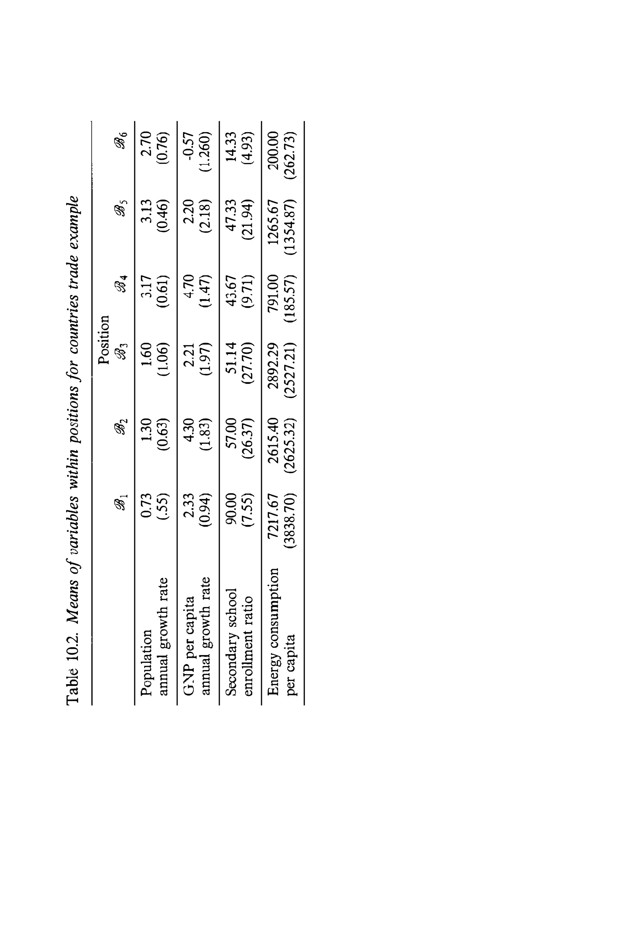
above (n,n2n6n, and n2n3n6n2) are of this type, and are allowed under
clustering (since they have three, not one, negative lines).
Clustering is less strict than balance. With clusterability, actors can
be partitioned into more than two clusters. If there is more than one
pair of actors with negative lines, then these actors are segregated into
different clusters. Specifically, if there is a triple of actors in a cycle
containing three negative lines, these three actors can be partitioned into
three different clusters. The negative lines will be between clusters. Such
a partitioning is not possible with balance, since there can be only two
subsets of actors. We should note that this theorem is quite general, since
it can be applied to signed graphs that are not necessarily complete. And
clusterability allows the sign of a cycle of length 3 to be negative.
Consider now a complete signed graph. The following theorem ex­
tends clusterability to complete signed graphs; its last condition is very
important. Again, it comes directly from Davis (1967).
Theorem 6.2 Thefollowingfour statements are equivalentfor any
complete signed graph:
• The graph is clusterable.
• The graph has a unique clustering.
6.2 Clusterability 237
• The graph has no cycle (ofany length) with exactly one negative
line.
• The graph has no cycle oflength 3 with exactly one negative line.
When the signed graph is complete, it is now possible to have a unique
clustering. Note, also, the last condition of the theorem. The lack of some
lines between nodes in a signed graph (as in Figure 6.5) makes it more
difficult to check for clusterability, and if such a graph is clusterable, we
have no guarantee that the clustering is unique. Lack of completeness
prevents us from guaranteeing a unique clustering. A clusterable complete
signed graph has a unique clustering, and this clustering can be verified
by looking just at all the triples. As Davis (1979) notes, referring to the
last condition concerning triples, ". . . 'threezies' were the key to the whole
thing,"
Flament (1963) proved that a complete graph is balanced if and only
if all its cycles of length 3 are balanced (that is, if such cycles all
have positive signs). Davis' clustering theorems, coupled with Flament's
(1963) finding that the properties of triples were sufficient to assess
the balance of a complete signed graph, led to nearly two decades of
research on statistical and deterministic models for triples. Through these
theorems, the properties of the triples of nodes in a graph tell us whether
theoretically important structural properties are present. The prominent
methodology for triples arising from this research will be discussed at
length in Chapter 14.
We should note that these theorems and this research focus only
on signed graphs. One can easily extend these theorems to signed
digraphs (representing a set of actors and a signed directional relation)
by looking at semicycles within the digraph. One need only replace the
terms "'graph," "nondirected," and "cycle" with the tenus "digraph,"
"directed," and "semicycle" in Theorems 1 and 2 and the following
discussions.
The uniqueness of the clusters is an important feature of clusterable
complete signed graphs. There is only one way to form these clusters.
If the graph is not complete but is clusterable, there may be more than
one acceptable way to form the clusters. Complete graphs are quite rare
in practice; thus, good methods for finding "good" sets of clusters from
not complete graphs are very important.
If the signed graph (or digraph) under study is not complete, then (as
stated by the first clusterability theorem) one has to look at all cycles,
not just those of length 3. The absence of cycles of length 3 that have
238 Structural Balance and Transitivity
just one negative line is a necessary, but not a sufficient, condition for
clusterability. If one can show that some of these cycles contain single
negative lines or arcs, then the (di)graph is not clusterable, and one need
not proceed to check cycles of longer length.
Signed graphs for which all cycles of length 3 meet the criteria of
the theorem, but cycles of longer length do not, are viewed as limited
clusterable, and are discussed by Harary, Norman, and Cartwright (1965).
Cartwright and Harary (1979) refer to a signed (di)graph whose nodes
can be partitioned into S subsets as an S-clusterable (di)graph. Balanced
(di)graphs are 2-clusterable.
Consider briefly graphs and digraphs that have no cycles. Such graphs
can be quite sparse and vacuous with respect to properties such as balance
and clusterability. If a (di)graph does not meet any of the conditions for
testing such properties, it is referred to as vacuous. Graphs and digraphs
are called vacuously balanced or vacuously clusterable by Cartwright and
Harary (1956) if they have no cycles or semicycles at all. Such structures,
such as a triple of nodes with just two positive lines, are vacuous, clearly
lacking the "tension" of unbalanced graphs or the "pleasantness" of
balanced ones.
One can construct and calculate iudices of clusterability analogous to
the indices of balance discussed earlier in this chapter. There are line
indices and cycle indices. There are also a variety of generalizations
of clusterability, which we discuss later in this chapter. There are also
extensions of these theoretical ideas to signed,valued graphs; for example,
see Cartwright and Harary (1970) and Kaplan (1972).
6.2.2 Summary
Indeed, triples are key. In brief, all balanced signed (di)graphs are
c1usterable, bnt clusterable signed (di)graphs may or may not be balanced.
And if the signed (di)graph is complete, one need only check cycles of
length 3 for verifying balance, and hence clusterability. For balance,
cycles of length 3 with three negative lines are a problem. Such cycles
are allowed for c1usterability, but not balance.
Note how the (-)(-)(-) cycle is allowed with clusterability, but not
with structural balance. The three actors must be placed into three distinct
subsets (since none of them have positive ties with each other), but this is
impossible with structural balance. Only two subsets are allowed, so one
of them would have to contain two actors with a negative relationship.
6.3 Generalizations of Clusterability 239
In a partition into clusters, clusterability allows these three actors to be
completely separated.
6.3 Generalizations of C1usterability
With these clusterability theorems in hand, a number of researchers
embarked on empirical investigations. Questions such as how common
clusterable signed (di)graphs are, and whether such signed (di)graphs
were balanced needed answers. Such investigations required surveying
many sociomatrices obtained from diverse sources. Further, the empirical
studies had to be accompanied by statistical models that allowed those
interested to study whether departures from theoretical models such as
clusterability were "statistically large."
The necessary statistical techniques are beyond the scope of the current
chapter. We will return to a study of triples and balance, and its successor,
transitivity, in Chapter 14. But we can report here how the theorems of
clusterability were generalized due to unexpected empirical evidence.
6.3.1 Empirical Evidence
Leinhardt (1968, 1973), Davis and Leinhardt (1968, 1972), and Davis
(1970) gathered nearly 800 sociomatrices from many different sources,
and discovered a few interesting facts. First, they found that many rela­
tions measured were directional. The recommended strategy of focusing
on semicycles in such structures was difficult to implement. Secondly,
asymmetric dyads, in which one actor chooses another actor, but the
choice is not reciprocated, were very common. The ideas of balance
and clusterability needed to be modified to take such situations into
account (rather than ignoring the directionality of these arcs, which was
the current practice when attention is focused on semicyc1es). Thirdly.
they found that signed relations were rather rare. Thus, they decided to
modify the theories of balance and clusterability for signed directional
relations. When these new theories were later found lacking, Holland
and Leinhardt (1971) revised them to unsigned directional relations.
Davis and Leinhardt also found that in some digraphs, one subset of
actors chose a second, while actors in this second subset chose members
of a third subset. The clusters of actors appeared to be ranked, or
hierarchical in nature, with the actors "on the bottom" choosing those
"at the top" (but not vice versa).
240 Structural Balance and Transitivity
6.3.2 ORanked Clusterability
Davis and Leinhardt (1968) consequently presented a concept of ranked
clusters, for complete signed directed graphs. Abandoning balance and
clusterability allowed them to focus on the sixteen possible triples that are
possible with this type of digraph. The sixteen are shown in Figure 6.6.
Notice that this idea can only be applied to complete digraphs, so that
every pair of nodes has two arcs between them, both of which have a
sign. Actor j must have either a positive or a negative tie to actor j, and
vice versa.
Theory slates that one need only examine triples when studying clus­
terability for complete signed graphs. The ranked clusterability mode�
which is discussed in detail by Davis and Leinhardt (1968), also states
that for such relations, one need only check threesomes. There are sixteen
possible kinds of threesomes that can arise in a complete signed digraph.
These sixteen, which are shown in Figure 6.6 (adapted from a figure in
Leik and Meeker 1975), are made up of only three kinds of dyads: ++
dyads, in which both arcs in the dyad have positive signs; -- dyads,
in which both arcs in the dyad have negative signs; and +- dyads, in
which one arc has a "+" and one has a "-".
Davis and Leinhardt (1972) state:
Relations of the sort we have called [+-] are assumed to connect
persons in different levels, while [the otherdyadic] relations are assumed
to connect persons in the same level. Further, we assume that in pairs
connected by [+-] relations, the recipient of the positive relationship
is in the higher level. (page 220)
They continue,
[++] relations are assumed to connect persons in the same [cluster1
within a level. [--] relations are assumed to connect persons in
different cliques within a leveL (page 220)
These two quotes nicely summarize which types oftriads are possible, and
which ones are not according to the postulates of ranked clusterability
for complete signed digraphs. In brief, ranked clusterability postulates
that ++ dyads occur only within clusters and -- dyads only between
clusters at the same level of the hierarchy or order of clusters. The
interesting +- dyads also occur between clusters, but at different levels.
Thus, actors in a lower cluster should have positive ties to actors in
a higher-ranked cluster and negative ties to actors in a lower-ranked
cluster. One can see how such a model postulates that "lower" clusters
of actors choose upwardly.
6.3 Generalizations of Clusterability
1"�' 2. .. _ _-II
- - - »-
3.
4.
,1,- - �.. - _ .
n' ,
- - ->'. - _ .
//',5. _ _ _>­
� - -
,i�,8.
=
9. /�
,1,t11 . U� - -
16. ,l}-
241
Fig. 6.6. The sixteen possible triads for ranked c1usterability in a com­
plete signed graph
242 Stnlelural Balance and Transitivity
Ranked cluslerability, in which the positive arcs emanating to or
from the nodes in [+-] dyads are postulated to "point" in the same
direclion, slales that the triples numbered 2, 10, 1 1, 12, 13, 14, 15, and
16 of Figure 6.6 should not occur in practice. These "miserable" eight
(Davis 1979) depart from both clusterability and ranked clusterability.
The empirical study of the 800 sociomatrices in the Davis/Leinhardt
soeiomctric data bank found that the vast majority of triples were not
of Ihese eight types (as reported in the reminiseenses of Davis 1979).
Unfortunately, triple 2, which is not allowed, was quite common. Davis
and Leinhardt (1972) concluded that
. . . we may say that we have had some success in showing that [+-]
relationships tend toward a rank structure and some success in showing
that C++] and [--] relations tend toward clusterability, but we have
had more limited success in showing how these two "structures" are
integrated to make a coherent whole. (page 249)
Not only was triple 2 quite common, but so was triple 16. As Davis (1979)
notes, therewas strong empirical evidence for 6/8th's of a theorem. These
two triples are quite common in positive affect relations which are in
an "early" development stage; that is, assuming that the relation under
study will change over time, these triples contain dyads which might
evolve into triples which are not prohibited.
This ranked clusterability model was quite elegant, but little used. The
ideas were quickly modified to account for another finding from the
study of the 800 sociomatrices in the Davis/Leinhardt sociometric data
bank - signed digraphs just are not very commonly collected.
The lack of signed graphs or digraphs in the 800 sociomatrices is not
surprising. The common technique for measuring affective relations (see
Chapter 2) is simply to pose only two alternatives to each actor about
every other actor: presence or absence of the tie in question. Davis
and associates clearly needed an approach that could handle non-signed,
directional relations. Adaptation of the "pre-1968" ideas to non-signed
relations did not come until consideration of transitivity, found first in
Holland and Leinhardt (1971). The first generalizations of clusterability
continued to focus on signed relations.
6.3.3 Summary
Holland and Leinhardt (1970) were the first to suggest the extension of
these ideas to non-signed directional relations. To turn ranked cluster­
ability for complete signed digraphs into an equivalent idea for digraphs
6.4 Transitivity 243
without signs is quite simple. We take the idea of ranked clusters for
complete signed digraphs, and do not consider arcs with negative signs.
Then, any arc with a sign of "-" is removed from the signed digraph. We
then drop the positive signs from the remaining arcs. The assumption is
that the relation under study is the "positive" part of the signed relation
- for example, we study only "like," "not like," and "dislike." Figure 6.7
shows the triples of Figure 6.6, without the negative arcs. The triples
arising from directional relations are commonly referred to as t/'iads,
since we consider the threesome of nodes, and all the arcs between them.
We note that the two problematic triads from ranked clusterability
found empirically to be quite common have one and five arcs. These
are the triads numbered 2 and 16 in Figure 6.7. Holland and Leinhardt
showed that ranked clusterability is a special cilse of a more general set
of theorems which naturally blend balance, clusterability, and ranked
clusterability. Their partially ordered clusterability leads naturally to a
consideration of the concept of transitivity.
Holland and Leinhardt (1971) reviewed the postulates of balance the­
ory, clusterability, and ranked clusterability, as well as transitive tourna­
ments (Landau 1951a, 1951b, and 1953; Hempel 1952), and proposed
the very general concept of transitivity to explain social structures. Tran­
sitivity includes all the earlier ideas as special cases. From a transitive
digraph, one can obtain balanced, clusterable, and ranked clusterable
graphs by making various assumptions about reciprocity and asymmetry
of choices. During the past two decades, evidence has accumulated that
transitivity is indeed a compelling force in the organization of social
groups. We now present this idea.
6.4 Transitivity
We turn our attention to a triple of actors, i, j, and k, and the ties
between them. We state:
Definition 6.4 The triad involving actors i, j, and k is transitive if
whenever i --> j and j --> k then i --> k.
If either of the two conditions of this statement is not met (that is,
if i +- j and/or j +- k), then the triple is termed vacuously transitive.
Vacuously transitive triples are neither transitive nor intransitive. Note
how the focus has shifted from cycles in signed graphs to semicycles in
signed digraphs to transitive triads in ordinary digraphs.
244 Structural Balance and Transitivity
Triad
-
I. _ -
/
-
2. _ -
-
/3. _ _
-
/4. _ _
j
-
5. / -
/
-
6. • __ •
/
-
7. •� .
-
8/:).
Triad
-
9 D.
/10. - -
-
11.
/---
/
-
12. •�.
-
13. •�.
/14. •�.
-
/I15. _= _
-
16. L).
Fig. 6.7. The sixteen possible triads for transitivity in a digraph
6.4 Transitivity 245
From this definition we have the following theorem:
Theorem 6.3 A digraph is transitive if every triad it contains is
transitive.
We note that if a transitive digraph has no asymmetric dyads - that is, if
all choices are reciprocated - then it is clusterable. Clusterable digraphs
require mutual dyads to be within and null dyads to be between clusters.
Thus, clusterability is a special case of transitivity. Ranked clusterable
digraphs are also transitive. In fact, transitivity is the most general idea
of this type for graphs and digraphs.
Refer again to Figure 6.7. The following triads are transitive: 6, 7, 8, 9.
Triads 1, 2, 3, 4, 5 are vacuously transitive. They do not contain enough
arcs to meet the conditions of the theorem, so cannot be transitive or
intransitive. Triads 10, 11, 12, 13, 14, 15, 16 are intransitive. Vacuously
transitive triads can occur and the digraph itself can still be transitive.
Now, rather than eight "miserable" triples from ranked clusterability,
there are only seven intransitive triads.
Notice that Definition 6.4 is stated for ordered triples of actors. Thus,
we must look at ordered triples rather than triads. Note also that each
threesome of actors consists of six distinct ordered triples of actors. Some
of these triples may have transitive choices, as defined in Definition 6.4,
while others may be intransitive. Still others may be vacuously transitive.
A triple must be of one of these types. For the triad itself to be labeled
transitive, all ordered triples of actors present in a triad must be either
transitive or vacuously transitive. If any one of the triples is intransitive,
so is the triad.
For example, look at triad 16 in Figure 6.7. As is the case with all triads,
triad 16 has six triples. This triad, along with its triples and their statuses,
arc listed in Figure 6.8. Three of the triples are transitive, while one of
them (the second) is not. The other two triples are vacuously transitive
(for example, the first triple, njnjnk, is neither transitive nor intransitive
since actor i does not have a tie to actor j). The second triple, n,nknj, is
clearly intransitive, since nj ---+ nk, nk ---+ nj, but nj -f+ nj. Thus, this triad
is considered intransitive because of this single intransitive triple. The
number of transitive and/or intransitive triples within a particular type
of triad is very important when quantitatively and statistically assessing
the amount of transitivity in a digraph. We discuss this issue in much
greater detail in Chapter 14.
246 Structural Balance and Transitivity
• ,
nj Triad 16
Triple #1 ; ni nj nk
nl -f+ nj 1'Ij -l> nk nj -Jo nk
Triple #2 : n,. nk nj
ni - nk nk --+ nj 1'Ij -f+ nj
Triple #3 : Hj ni nk
nj - ni nj -) nk nj -)0 nk
Triple #4 : nj nk ni
nj -+ nk nk -+ nj nj --). nj
Triple #5 : nk nj nj
nk -+ ni ni + nj nk -+ nj
Triple #6 : nk nj ni
11k --+ nj nj _ nj nk -+ ni
•
nk
Vacuously transitive
Intransitive
Transitive
Transitive
Vacuously transitive
Transitive
Fig. 6.S. The type 16 triad, and all six triples of actors
The generality of transitivity can be seen, for example, by looking
at triad 2 from Figure 6.7. This triad, which is not allowed under..
ranked c1usterability, has just a single asymmetric dyad, so it is vacuously
transitive. Vacuously transitive triples are allowed under transitivity, so
type 2 triads can arise, without invalidating the idea.
The other triad that was problematic for ranked dusterability was triad
16, which we described in detail above. Davis and Leinhardt showed that
this triad occurred far too frequently. But this triad is almost transitive.
Only one of its six triples is intransitive. So, the presence of this 5/6th's
transitive/vacuously transitive triad in a data set is not such a big deal
(assuming transitivity is operating).
Holland and Leinhardt (1972) provide strong, statistical evidence that
transitivity is a very important structural tendency in social networks.
By relying on the Davis/Leinhardt sociometric data bank, Holland and
Leinhardt present evidence of transitive social structure. Holland and
Leinhardt (1975, 1978, 1979) and Johnsen (1985, 1986) show that transi­
tivity is one of many "nUll hypotheses" that can be tested by examining
triads and the triples they contain.
6.5 Conclusion 247
The statistical methodology for determining how many intransitivities
can be present in an actual data set, before concluding that transitivity
does not hold, is discussed in Chapter 14.
6.5 Conclusion
Transitive digraphs (called t-graphs by Holland and Leinhardt 1971), and
the mathematical methods based on them are quite important. These
structures, methods, and theorems unified over two decades of theorizing
about balance, clusterability and its generalizations, and transitivity, in
sociology and social psychology. Transitivity has been shown to be a key
structural property in social network data. In fact, many recent methods
center on finding "what else" remains in a data set after "removing"
tendencies toward transitivity. The idea of a transitivity bias or structural
tendency in social network data was discussed as early as Rapoport
(1953, 1963) and Fararo and Sunshine (1964) (see also the discussion of
random and biased nets in Fararo and Skvoretz 1984, 1987; Skvoretz
1985, 1990). There are, of course, other tendencies that can occur in a
social network - in fact, we spend much of the remainder of this book
describing and quantifying them. But after tendencies toward reciprocity
were discussed in the 1940's, balance and its generalization, transitivity,
were the earliest theories to play an important part in social network
analysis.
As we have discussed in this chapter, Cartwright and Harary (1956)
used graph theory to quantify Heider's (1946) balance theory, and pro­
posed a theorem that implied that a set of actors, if balanced, could be
partitioned into two subsets. The data, unfortunately, had to be from a
signed graph in order to apply this idea. Davis (1967) recognized that
the decomposition of a set of actors into just two subgroups was not
empirically likely; consequently, he expanded upon structural balance by
proposing theorems that showed under what conditions such partitions
could arise. Davis's ranked clusterability included balance theory as a
special case, and thus seemed far more appropriate for social network
data. Again, the restriction to signed graphs was quite a limitation;
Davis and Leinhardt's (1972) empirical searches recognized that most
social network data included unsigned, rather than signed, relations.
With this empirical knowledge, Davis and Leinhardt (1968) combined
the common tendency toward clustering with a second structural tendency
toward ranking or differential status, to show how directional relations
could generate structures resembling hierarchically arranged clusters.
248 Structural Balance and Transitivity
Going a step further, concentrating on the" very _C9mmon directional,
unsigned relations, Holland and Leinhardt (1970) showed how ideas
about partially ordered clusters, generalizing ranked clusterability, lead
naturally to transitivity, During the past two decades, research, such
as Mazur (1971), Davis, Holland, and Leinhardt (1971), Holland and
Lcinhardt (1973, 1979), Killworth (1974), Frank (1979a), Frank and
Harary (1979, 1980, 1982), and Johnsen (1985, 1986), has continued
the development of transitivity, but the major efforts can be found in
the work of Heider, Cartwright, Harary, Davis, Holland, and Leinhardt
during the period 1945-19n
Many researchers have studied the implications of balance theory and
transitivity for l'iocial structures: to name hut a few, Morrissette (1958),
Rodrigues (1967, 1981), Horsfall and Henley (1969), Johnsen (1970),
Wellens and Thistlethwaite (1971a, 1971b), Crano and Cooper (1973),
Rodrigues and Ziviani (1974), Willis and Burgess (1974), Mower White
(1977, 1979), Moore (1978), Tashakkori and Insko (1979), Newcomb
(1981), Feld and Elmore (1982a), Rodrigues and Dela Coleta (1983),
Chase (1982), Gupta (1985, and references therein), Mohazab and Feger
(1985), especially the review ofZajonc (1968), and the work ofFararo and
Skvoretz mentioned earlier, Transitivity nnderlies many social network
methods. It will arise in Chapters 10 and especially 14, where we present
statistical methods for determining the extent of transitivity in a social
network. The ideas presented in Chapter 6 were important not only to
network theorists, but to many methodologists.
We note in conclusion that while this small set of graph theorists, so­
ciologists, social psychologists, and statisticians were working on mathe­
matical models of balance, clusterability, and transitivity, other method­
ologists were busy studying about cliques and cohesive subgroups. This
area of research is described in the next chapter.
7
Cohesive Subgroups
One of the major concerns of social network analysis is identification of
cohesive subgroups of actors within a network. Cohesive subgroups are
subsets of actors among whom there are relatively strong, direct, intense-,-­
frequent or positive ties. These methods attempt, in part, to formalize
the intuitive and theoretical notion of social group using social network
properties. However, since the concept of social group as used by social
and behavioral scientists is quite general, and there are many specific
properties of a social network that are related to the cohesiveness of
subgroups, there are many possible social network subgroup definitions.
In this chapter and the next we discuss methods for finding cohesive
subgroups of actors within a social network. In this chapter we discuss
methods for analyzing one-mode networks, with a single set of actors
and a single relation. In Chapter 8 we continue the discussion of
cohesive subgroups and related ideas, but focus on affiliation networks.
Affiliation networks are two-mode networks consisting of a set of actors
and a set of events. Cohesive subgroups in one-mode networks focus
on properties of pairwise ties, whereas cohesive subgroups in two-mode
affiliation networks focus on ties existing among actors through their
joint membership in collectivities. Thus, one major difference between
this chapter and the next is whether one-mode or two-mode data are
being analyzed.
We begin with an overview of the theoretical motivation for studying
cohesive subgroups in social networks and discuss general properties of
cohesive subgroups that have influenced network formalizations. We then
discuss how to assess the cohesiveness of network subgroups, and extend
subgroup methods to directional relations and to valued relations. The
final section of this chapter briefly discusses alternative approaches for
studying cohesiveness in networks using multidimensional scaling and
249
250 Cohesive Subgroups
factor analysis. Most of the methods discussed in this chapter are based
on graph theoretic ideas. and use graph theoretic concepts and notation.
Thus, it might be useful to review Chapter 4 before reading the rest of
this chapter.
7.1 Background
In this section we discuss the theoretical background for social groups,
briefly outline some ways to conceptualize cohesive subgroups, and review
key notation and graph theoretic concepts that are used to study cohesive
subgroups.
7.1.1 Social Group and Subgroup
Many authors have discussed the role of social cohesion in social expla­
nations and theories (Burt 1984; Collins 1988; Erickson 1988; Friedkin
1984). Friedkin examines the use of network cohesion as an explanatory
variable in sociological theories, especially for studyinR the emergence of
consensus among members of a group: .
Structural cohesion models are founded upon the causal propositions
that pressures toward uniformity occur when there is a positively val­
ued interaction between two persons; that these pressures may OCCUr by
being "transmitted" through intermediaries even when two persons are
not in direct contact; and that such indirect pressures toward unifor­
mity are associated with the number of short indirect communication
channels connecting the persons. (1984, page 236)
Consequently, according to this idea, one expects greater homogeneity
among persons who have relatively frequent face-to-face contact or who
are connected through intermediaries, and less homogeneity among per­
sons who have less frequent contact (Friedkin 1984). In his review of
sociological theory, Collins (1988) .also states the importance of cohesion
in social network analysis:
The..more tightly that individuals are tied into a network� the more they
are affected by group standards . . . . (page 416)
Collins continues, noting that
Actually, there are two factors operating here, which we can see from
network analysis: how many ties an individual has to thlj group and how
dosed the entire group is to out!nd.era.. iSolated and tightly connected
groups make up a clique; within such highly cohesive groups, individuals
tend to have very homogeneous beliefs. (page 417)
7.1 Background 251
Cohesive subgroups are theoretically important according to these the­
ories because of social forces operating through direct contact among
subgroup members, through indirect conduct transmitted via intermedi­
aries, or through the relative cohesion within as compared to outside the
subgroup. Such theories provide motivation for cohesive subgroup meth­
od� for one-mode social networks (in which ties are measured between
pairs of actors). These ideas are all used to study cohesive subgroups in
social networks.
The notions of social group, subgroup, clique, and so on are widely
used in the social sciences, particularly in social psychology and sociology.
Although the notion of social group has received widespread attention
in the social sciences, researchers often use the word without giving
it a precise formal definition. As noted by Freeman (1984, 1992a)
and Borgatti, Everett, and Freeman (1991) authors often assume that
since "everybody knows what it means" it can be used without precise
definition. Freeman reviews the history of the concept of group in
sociology with special attention to network formalizations of this concept
(Freeman 1992a).
Many network researchers who have developed or reviewed methods
for cohesive subgroups in social networks have noted that these methods
attempt to formalize the notion of social group (Seidman and Foster
1978a, 1978b; Alba and Moore 1978; Mokken 1979; Burt 1980; Freeman
1984, 1992a; Sailer and Gaulin 1984). According to these authors, the
concept of social group can be studied by looking at properties of
subsets of actors within a network. In social network analysis, the notion
of subgroup is formalized by the general property of cohesion among
subgroup members based on specified properties of the ties among the
members. However, since the property of cohesion of a subgroup can
be quantified using several different specific network properties, cohesive
subgroups can be formalized by looking at many different properties of
the ties among subsets of actors.
Although the literature on cohesive subgroups in networks contains
numerous ways to conceptualize the idea of subgroups, there are four
general properties of cohesive subgroups that have influenced social
network formalizations of this concept. Briefly, these are:
• The mutuality of ties
• The closeness or reachability of subgroup members
• The frequency of ties among members
252 Cohesive Subgroups
• The relative frequency of ties among snbgroup members com­
pared to non-members
Subgroups based on mutuality of ties require that all pairs of subgroup
members "choose" each other (or are adjacent) ; subgroups based on
reachability require that all subgroup members be reachable to each
other, but not necessarily adjacent; subgroups based on numerous ties
require that subgroup members have ties to many others within the
subgroup; and subgroups based on the relativ" density or frequencv of
ties require that subgroups be relatively cohesive when compared to the
remainder of the network. Successive definitions weaken the first notion
of adjacency among all subgroup members. These general subgroup ideas
lead to methods that focus on different social network properties. Thus,
our discussion in this chapter is divided into sections, each of which takes
up methods that are primarily motivated by one of these ideas.
In contrast to these ideas that focus on ties between pairs of actors in
one-mode networks, some cohesive subgroup ideas are concerned with
the linkages that are established among individuals by virtue of their
common membership in collectivities. These ideas motivate methods for
studying affiliation networks, which we discuss in Chapter 8.
Before we present the subgroup methods for one-mode networks, let
us review some basic concepts and definitions from graph theory.
7.1.2 Notation
Our presentation of notation here is intentionally brief, since these ideas
were covered in detail in Chapters 3 and 4. To start, we will limit our
attention to graphs, and thus, to dichotomous nondirectional relations.
We begin with a graph, 'If, consisting of a set of nodes, %, and a set
of lines, :.e. Each line connects a pair of nodes in 'If. Two nodes that are
connected by a line are said to be adjacent. A node generated subgraph,
'If" of 'If, consists of a subset of nodes, %" where %, ,; %, along with
the lines from :.e that link the nodes in 'If,. We will refer to a subset of
nodes as a subgroup or subset, and the nodes along with the lines among
them as a subgraph. A graph is complete if all nodes are adjacent; that
is, if each pair of nodes is connected by an line. Similarly, a subgraph,
ris, is complete if all pairs of nodes in it are adjacent.
A path connecting two nodes is a sequence of distinct nodes and lines
beginning with the first node and terminating with the last. If there
is a path between two nodes then they are said to be reachable. The
7.2 Subgroups Based on Complete Mutuality 253
length of a path is the number of lines in it. A shortest path between
two nodes is called a geodesic, and the (geodesic) distance between two
nodes, denoted by d(i, j), is the length of a shortest path between them.
The diameter ofa graph is the length of the longest geodesic between any
pair of nodes in the graph. In other words, the diameter of a graph is the
maximum geodesic distance between any pair of nodes; max(d(i,j))i for
n;, nj E .11". Similarly, the diameter ofa subgraph can be defined as the
longest geodesic between two nodes within the subgraph. The diameter
of a subgraph is defined on the subset of nodes and lines that are present
in the subgraph.
A graph is connected if there is a path between each pair of nodes in
the graph. A subgraph is connected if there is a path between each pair
of nodes in the subgraph, and the path contains only nodes and lines
within the subgraph. The degree of a node, d(i), is the number of nodes
that are adjacent to it. The degree of node i in subgraph '#, is denoted
by d,(i), and is defined as the number of nodes within the subgraph that
are adjacent to node i.
A subgraph is said to be maximal with respect to some property (for
example, completeness) if that property holds for the subgraph, but does
not hold if additional nodes and the lines incident with them are added
to the subgraph. If a subgraph is maximal with respect to a property,
then that property holds for the subgraph, '#" but not for any larger
subgraph that contains '#, (Mokken 1979). For example, a component of
a graph is a maximal connected subgraph (Hage and Harary 1983). The
presence of two or more components in a graph indicates that the graph
is disconnected.
We can now define some interesting subgroup ideas using these graph
theoretic concepts.
7.2 Subgroups Based on Complete Mutuality
The earliest researchers interested in cohesive subgroups gathered and
studied sociometric data on affective ties, such as friendship or liking
in small face-to-face groups, in order to identify "cliquish" subgroups.
Network data on friendship nominations often give rise to directional
dichotomous relations. Festinger (1949) and Luce and Perry (1949)
argued that cohesive subgroups in directional dichotomou� relations
would be characterized by sets of people among whom all friendship
choices were mutual. Specifically, Luce and Perry and Festinger proposed
that a clique for a relation of positive affect is a subset of people among
254 Cohesive Subgroups
whom all choices are mutual, and no other people can be added to the
subset who also have mutual choices with all members of the subset.
This definition of a clique is appropriate for a directional dichotomous
relation.
The clique is the foundational idea for studying cohesive subgroups in
social networks. Graph theory provides a precise formal definition of a
clique that is appropriate for a nondirectional dichotomous relation.
7.2.1 Definition of a Clique
A clique in a graph is a maximal complete subgraph of three or more
nodes. It consists of a subset of nodes, all of which are adjacent to
each other, and there are no other nodes that are also adjacent to all of
the members of the clique (Luce and Perry 1949; Harary, Norman, and
Cartwright 1965). The restriction that the clique contain at least three
nodes is included so that mutual dyads are not considered to be cliques.
One can think of a clique as a collection of actors all of whom "choose"
each other, and there is no other actor in the group who also "chooses"
and is "chosen" by all of the members of the clique.
The clique definition is a useful starting point for specifying the formal
properties that a cohesive subgroup should have. It has well-specified
mathematical properties, and also captures much of the intuitive notion
of cohesive subgroup; however, it has limitations, which we discuss below.
Figure 7.1 shows a graph and a listing of the cliques contained in it.
The reader can verify that these subgraphs are in fact cliques, and that
there are no remaining cliques in the graph.
Notice that cliques in a graph may overlap. The same node or set of
nodes might belong to more than one clique. For example, in Figure 7.1
node 3 belongs in all three cliques. Also, there may be nodes that do not
belong to any cliques (for example node 7 in Figure 7.1). However, no
clique can be entirely contained within another clique, because if it were
the smaller clique would not be maximal.
7.2.2 An Example
We will use the example of the relations of marriage and business among
Padgett's Florentine families to illustrate cohesive subgroups throughout
this chapter. Recall that both of these relations are dichotomous and
nondirectional. We used the network analysis programs GRADAP 2.0
7.2 Subgroups Based on Complete Mutuality 255
2 7
3
1 ._------.t----__ 4
S 6
cliques: {1,2,3}, {I, 3, S}, and {3,4,S,6}
Fig. 7.1. A graph and its cliques
(Sprenger and Stokman 1989) and UCINET IV (Borgatti, Everett, and
Freeman 1991) to do the subgroup analyses described in this chapter.
First consider the relation of marriage among these families. For the
marriage relation there are three cliques:
• Bischeri Peruzzi Strozzi
• Castellani Peruzzi Strozzi
• Medici Ridolfi Tornabuoni
Only seven of the sixteen families in this network belong to any clique
on the marriage relation. Furthermore, the cliques are small; each clique
contains only the minimum three families. By definition, there has been
a marriage between all pairs of families in each clique. Notice that the
first two cliques contain two members in common (Peruzzi and Strozzi),
and differ only by a single member. However, the four families, Bischeri,
Castellani, Peruzzi and Strozzi, do not form a clique because there is no
marriage tie between Castellani and Bischeri.
For the business relation there are five cliques:
• Barbadori Castellani Peruzzi
• Barbadori Ginori Medici
• Bischeri Guadagni Lamberteschi
• Bischeri Lamberteschi Peruzzi
• Castellani Lamberteschi Peruzzi
256 Cohesive Subgroups
Eight of the sixteen families belong to at least one clique On the business
relation, and some families (for example Lamberteschi, Bischeri, and
Peruzzi) belong to several cliques on this relation. As we saw with the
marriage relation, the cliques are small (no more than three members)
and there is considerable overlap among them. However, the cliques that
are present in the business relation are different from the cliques that are
present in the marriage relation.
7.2.3 Considerations
A clique is a very strict definition of cohesive subgroup. In fact, Alba
(1973) calls it "stingy." The absence of a single line, or in sociometric
terms, the absence of a single tie or "choice," will prevent a subgraph
from being a clique. In a sparse network there may be very few cliques (as
with the marriage relation among the Florentine families). In addition,
the sizes of the cliques will be limited by the degree of tbe nodes. This
can be a problem if the number of ties that an actor can have is limited
by the data collection design. For example, in a sociometric study using
a fixed choice design in which respondents are asked to list their three
best friends, each person can be adjacent to at most three other people.
Thus there can be no clique with more than four members. In general, if
actors are restricted to k ties, then there can be no clique in the resulting
data that has more than k + 1 members.
Early researchers were concerned with methods for detecting cliques
in networks (Festinger 1949; Luce and Perry 1949; Luce 1950; Harary
and Ross 1957). More recently, researchers have realized tbat cliques
seldom are useful in analysis of actual data because the definition is too
strict. Actual data rarel,jl contain interestin& cliques, since the absence
of a single tie among subgroup members prevents the subgroup from
meeting the clique definition. In addition, cliques that do occur are often
quite smal� and overlap one another (as we have seen in the analysis of
Padgett's Florentine families).
An additional limitation of clique as a formalization of cohesive sub­
group is that there is no internal differentiation among actors within
a clique (Doreian 1969; Seidman and Foster 1978a, 1978b; Freeman
1992a, 1992b). Since a clique is complete, within tbe clique all members
are graph theoretically identical. All clique members are adjacent to all
other clique members, thus tbere are no distinctions among members
based on graph theoretic properties within the clique. If we expect that
the cohesive subgroups within a network should exhibit interesting in-
7.3 Reachability and Diameter 257
ternal structure, such as having some core actors who are more strongly
identified with the subgroup and other peripheral actors who are less
identified with it, then a clique might be an inappropriate definition of
cohesive subgroup.
On the other hand, some researchers working with large network data
sets (that include hundreds or even thousands of actors) have found that
there may be numerous, but largely overlapping, cliques in the group
(Alba and Moore 1978). In such cases, the cliques themselves might
not be very informative. Instead, the researcher might study the overlap
among the cliques. Studying how cliques overlap is one way to focus on
the differentiation or internal structure of subgroups within the network.
A recent paper by Freeman (1992b) describes how to use lattices (which
we define in Chapter 8) to study the overlap among cliques in social
network.
An active area of recent research is the development of methods to
extend the definition of cohesive subgroup to make the resulting sub­
groups more substantively and theoretically interesting. These methods
weaken the notion of clique so that the subgroups are less "stingy."
There are obviously numerous ways to loosen the definition by removing
required properties of a subgraph. These definitions describe subgraphs
that are not cliques, but rather, are "cliqueMiike" entItles. The '·tnck;�
is fo develop formal mathematical definitions that have known graph
theoretic properties, and also capture important intuitive and theoretiCal
aspects of cohesive subgroups. Two different structural properties have
been used to. rela.x the cliqlle notion: first, Luce (1950), and later Alba
(1973) and Mokken (1979), have used properties of reachability, path
distance, and diameter to extend the clique definition; second, Seidman
and Foster (1978a) and Seidman (1981b, 1983b) used nodal degree to
propose alternative cohesive subgroup ideas. Both of these ideas take
the clique as a starting point, and extend it by removing one or more
r�strictions_ We will descrihe each of these in turn.
7.3 Snbgroups Based on Reacbability and Diameter
Reachability is the motivation for the first cohesive subgroup ideas
that extend the notion of a clique. These alternative subgroup ideas are
useful if the researcher hypothesizes that important social processes occur
through intermediaries. For example, the diffusion of information has
been hypothesized to occur in this way (Erickson 1988). Conceptually,
there should be relatively short paths of influence or communication
258 Cohesive Subgroups
between all members of the subgroup. Subgroup members might not be
adjacent, but if they are not adjacent, then the paths connecting them
should be relatively short.
7.3.1 n-cliques
Recall that the geodesic distance between two nodes, denoted by d(i, j),
is the length of a shortest path between them. Cohesive subgroups based
on reachability require that the geodesic distances among members of
a subgroup be smalL Thus, we can specify some cutoff value, n, as
the maximum length of geodesics connecting pairs of actors within
the cohesive subgroup. Restricting geodesic distance among subgroup
members is the basis for the definition of an n-clique (Alba 1973; Luce
1950). An n-clique is a maximal subgraph in which the largest geodesic
distance between any two nodes is no greater than n. Formally, an
n-clique is a subgraph with node set .N" such that
d(i,j) :;; n for all n;,nj E .N, (7.1)
and there are no additional nodes that are also distance n or less from
all nodes in the subgraph.
When n = 1, the subgraphs are cliques, since all nodes are adjacent.
Increasing the value of n gives subgraphs in which longer geodesic
distances between nodes are permitted. A value of n = 2 is often a
useful cutoff value. 2-cliques are subgraphs in which all members need
not be adjacent, but all members are reachable through at most one
intermediary.
Let us look at an example to illustrate n-cliques. Figure 7.2, taken
from Alba (1973) and Mokken (1979), contains a single clique, {1, 2, 3},
which, by definition, is a 1-clique. In this graph, there are two 2-cliques:
{1, 2, 3, 4, 5} and {2, 3,4, 5, 6}. Notice that these two 2-cliques share four
of their five members. In addition, it is important to note that even
though we are using a maximum geodesic distance of n = 2 to find the
2-cliques, the first 2-clique ({I, 2, 3, 4, 5}) has a diameter of 3. The geodesic
between nodes 4 and 5 includes node 6, which is not a member of this
2-clique. Within this 2-clique, the shortest path between 4 and 5 is the
path 4, 2, 3, 5, which is oflength 3. Thus, n-cliques can be found in which
the intermediaries in a geodesic between a pair of n-clique members are
not themselves n-clique members.
7.3 Reachability and Diameter
1
2�----",, 3
4
6
2-c1iques: {1,2,3,4, 5} and {2, 3,4, 5,6}
2-c1an: {2, 3, 4, 5,6}
5
2-c1ubs : {1,2,3,4}, {1,2,3,5}, and {2,3,4, 5,6}
Fig. 7.2. Graph illustrating n-cliques, n-c1ans, and n-clubs
73_2 An Example
259
Let us return to the example of marriage and business relations among
Padgett's Florentine families to illustrate n-cliques. We used the program
GRADAP 2.0 (Sprenger and Stokman 1989) for this analysis. There are
thirteen 2-cliques in the marriage relation:
• Acciaiuoli Albizzi Barbadori Medici Ridolfi Salviati Tornabuoni
• Albizzi Bischeri Guadagni Lamberteschi Tornabuoni
• Albizzi Bischeri Guadagni Ridolfi Tornabuoni
• Albizzi Ginori Guadagni Medici
• Albizzi Guadagni Medici Ridolfi Tornabuoni
• Barbadori Castellani Medici Ridolfi Strozzi
• Barbadori Castellani Peruzzi Ridolfi Strozzi
• Barbadori Medici Ridolfi Strozzi Tornabuoni
• Bischeri Castellani Peruzzi Ridolfi Strozzi
• Bischeri Guadagni Peruzzi Ridolfi Strozzi
• Bischeri Guadagni Ridolfi Strozzi Tornabuoni
260 Cohesive Subgroups
• Guadagni Medici Ridolfi Strozzi Tornabuoni
• Medici Pazzi Salviati
There are four 2-cliques on the business relation :
• Barbadori Bischeri Castellani Lamberteschi Peruzzi
• Barbadori Castellani Ginori Medici Peruzzi
• Barbadori Ginori Medici Pazzi Salviati Tornabuoni
• Bischeri Castellani Guadagni Lamberteschi Peruzzi
Notice that the 2-cliques are both larger and more numerous than the
cliques found for both the marriage and business relations. Since the
definition of an n-clique is less restrictive than the definition of a clique,
when n is greater than I it is likely that a network will contain more
n-cliques than cliques. It is also likely that the n-cliques will be larger
than the cliques.
7.3.3 Considerations
There are several important properties of n-cliques, some of which limit
the usefulness of this cohesive subgroup definition. Since n-cliques are
defined for geodesic paths that can include any nodes in the graph,
two problems might arise: first, an n-clique, as a subgraph, may have a
diameter greater than n, and second, an n-clique might be disconnected.
The first problem arises because the requirement that nodes be connected
by paths of length n or less docs not require that these paths remain
within the subgroup (Alba 1973; Alba and Moore 1978). Geodesics
connecting a pair of nodes in an n-clique may include nodes that lie
outside of the n-clique. Thus, the diameter of the subgraph can be
larger than n. The second problem is that an n-clique may not even
be connected. Two nodes may be connected by a geodesic of n or less
which includes nodes out�ide the n-clique, and these two nodes may have
no path connecting them that includes only n-clique members. These
problems indicate that n-cliques are not as cohesive as we might like for
studying cohesive subgroups (Alba and Moore 1978; Mokken 1979).
7.3.4 n-clans and n-clubs
One idea to "improve" n-cliques is to restrict them so that the resulting
subgroups that are identified are more cohesive, and do not have the
problems of n-cliques. A useful restriction is to require that the diameter
73 Reachability and Diameter 261
of an n-clique be no greater than n. Mokken (1979) has described two
logical ways to do this. The first, which he calls an n-clan, starts with
the n-cliques that are identified in a network and excludes those n-cliques
that have a diameter greater than n. The second approach, called an
n-club, defines a new entity, a maximal n-diameter subgraph.
An n-clan is an n-clique in which the geodesic distance, dU, j), between
all nodes in the subgraph is no greater than n for paths within the
subgraph. The n-clans in a graph can be found by examining all n-cliques
and excluding those that have diameter greater than n. Any n-cliques that
include pairs of nodes whose geodesics require non-subgroup members
are excluded from consideration. The n-clans in a graph are those n­
cliques that have diameter less than or equal to n (Alba 1973; Mokken
1979). All n-clans are n-cliques.
An n-club is defined as a maximal subgraph of diameter n. That is, an
n-club is a subgraph in which the distance between all nodes within the
subgraph is less than or equal to n; further, no nodes can be added that
also have geodesic distance n or less from all members of the subgraph.
n-clubs are not necessarily n-cliques, though they are always subgraphs
of n-cliques.
Although conceptually similar, n-clans and n-clubs are somewhat dif­
ferent, as illustrated in Figure 7.2. This example is taken from Alba (1973)
and Mokken (1979), and illustrates the difference between n-cliques, n­
clans, and n-clubs. For this graph, taking n = 2 results in the following
sets:
• 2-cliques : {1,2, 3,4,5} and {2, 3,4,5,6}
• 2-clan: {2,3,4,5, 6}
• 2-clubs: {1, 2, 3, 4}, {1, 2, 3, 5}, and {2, 3,4, 5, 6}
First, consider the 2-cliques and 2-clans. Since the 2-clique {I, 2, 3, 4, 5}
has diameter greater than 2 (the distance from 4 to 5 is equal to 3) it
is not an 2-clan. The 2-clique {2, 3, 4, 5, 6} is a 2-clan since its diameter
is not greater than 2. Now, consider the 2-clubs. The 2-clubs {I, 2, 3,4}
and {I, 2, 3, 5} both have diameter equal to 2, and are maximal, since no
node can be added to either subgraph without increasing its diameter.
Notice that each of these 2-clubs is a subgraph of the 2-clique {I, 2, 3,4, 5}
(whose diameter is greater than 2). Finally, the 2-club {2, 3, 4, 5, 6} has a
diameter of 2 and is maximal.
As this example illustrates, 2-clubs are either 2-cliques, or are subgraphs
of 2-cliques. Mokken (1979) demonstrates that all n-clans are also n-
262 Cohesive Subgroups
cliques, and all n-clubs are contained within n-cliques. Furthermore, all
n-clans are also n-clubs, though there can be n-clubs that are not n-clans.
As Sprenger and Stokman (1989) have noted, "hardly anybody" has
used n-clans and n-clubs, and more research is needed on these cohesive
subgroup ideas. The n-clans in a social network are relatively easy to find
by examining the n-cliques, and eliminating those with diameter greater
than n. The n-c1ubs are difficult to find, and often routines for n-clubs
are not included in standard network analysis packages. Therefore, in
the following example we restrict our attention to n-clans.
An Example. We will use the marriage and business relations
for Padgett's Florentine families to illustrate n-clans. For the business
relation, all of the four 2-cliques have a diameter that is 2 or less, and
therefore these four 2-cliques are also 2-clans. For the marriage relation,
five of the 2-cliques have diameter greater than 2, so they are excluded
from the list of 2-clans. This leaves eight 2-clans:
• Acciaiuoli Albizzi Barbadori Medici Ridolfi Salviati Tornabuoni
• Albizzi Bischeri Guadagni Lamberteschi Tornabuoni
• Albizzi Ginori Guadagni Medici
• Albizzi Guadagni Medici Ridolfi Tornabuoni
• Barbadori Castellani Medici Ridolfi Strozzi
• Bischeri Castellani Peruzzi Ridolfi Strozzi
• Bischeri Guadagni Ridolfi Strozzi Tornabuoni
• Medici Pazzi Salviati
The difference between the 2-cliques and the 2-clans on the marriage
relation is that the five 2-cliques with diameter greater than 2 are excluded.
For example, the diameter of the 2-clique {Barbadori, Medici, Ridolfi,
Strozzi, Tornabuoni} is greater than 2, since the geodesic between Strozzi
and Barbadori (which is of length 2) includes Castellani (who is not in
this 2-clique).
7.3.5 Summary
The three definitions of cohesive subgroups discussed in this section are
primarily motivated by the property of reachability among the nodes in
a subgraph. An n-clique simply requires that there is some short path
(geodesic) between subgroup members, though this short path may go
outside the subgraph. An n-clique may be seen as too loose a definition
of cohesive subgroup, and restrictions requiring geodesic patbs to remain
7.4 Subgroups Based on Nodal Degree 263
within the subgroup can be applied by requiring the subgraph to have a
given maximum diameter. n-clubs and n-clans are two possible definitions
that have the desired restrictions.
As Erickson (1988) has noted, cohesive subgroup definitions based
on reacbability are important for understanding "processes that operate
througb intermediaries, sucb as the diffusion of clear cut and widely
salient information" (Erickson 1988, page 108). In studying network
processes such as information diffusion that "flow" through interme­
diaries, cohesive subgroups based on indirect connections of relatively
short paths provide a reasonable approach.
A related cohesive subgroup idea is influence among subgroup mem­
bers. This idea provides the motivation for Hubbell's (1965) adaptation
of economic input-output models to sociometric data. Hubbell argues
that ties between actors are "channels for the transmission of influence"
(1965, page 377). Influence occurs both through direct contact and
througb indirect cbains of contact via other actors. The goal is to iden­
tify subgroups of actors among whom there is a relatively strong mutual
influence, whether the influence is direct or indirect. Hubbell's approach
relies on measures of influence based on a weighting of adjacencies and
paths of influence, and a partitioning of actors based on the degree to
which subgroup members mutually influence each other.
In contrast, if one hypothesizes tbat network processes require direct
contact among actors, and perbaps repeated, direct, contact to several
actors, then a different cohesive subgroup definition is required. We turn
now to subgroup methods that study cohesive subgroups by focusing on
adjacency between actors, rather than on paths and geodesics.
7.4 Subgroups Based on Nodal Degree
In this section we describe cohesive subgroup ideas that are based on
the adjacency of subgroup members. These approaches are based on
restrictions 011 the millinlUm nUlnber of actors adjacent to each actor
in a subgroup. Since the number of actors adjacent to a given actor is
quantified by the degree of the node in a graph, these subgroup methods
focus on nodal degree. Subgroups based on nodal degree require actors to
be adjacent to relatively numerOUS other subgronp members. Thus, unlike
the clique definition that requires all members of a cohesive subgroup
to be adjacent to all other subgroup members, these alternatives require
that all subgroup members be adjacent to some minimum number of
other subgroup members.
264 Cohesive Subgroups
2
.-------�-------. 4
3
Fig. 7.3. A vulnerable 2-clique
Subgroups based on adjacency between members are useful for under­
standing processes that operate primarily through direct contacts among
subgroup members. For example, Erickson hypothesizes that "multiple
redundant channels of communication" will be related to the accuracy of
information and the recognizability of subgroups (Erickson 1988, page
108).
These definitions arise in part because of the "vulnerability" of n­
cliques. Seidman and Foster (1978) observed that n-cliques often are not
robust. One measures robustness by considering "the degree to which the
structure is vulnerable to the removal of any given individual" (Seidman
and Foster 1978, page 142). Robustness is often assessed using measures
of connectivity (see Chapter 4). Robust subgraphs are little affected by
the removal of individual nodes. For example, consider the 2-clique in
Figure 7.3 consisting of nodes 1,2,3, and 4. Although all pairs of nodes
are within path distance 2 of each other, these paths all contain node 3.
Node 3 is critical for the connections between other nodes. Furthermore,
1,2, and 4 are not connected to each other through any paths that do
not contain 3. This 2-clique is vulnerable to the removal of node 3.
The possible lack of robustness of n-cliques was one consideration that
led to the proposal of an alternative subgroup definition. This alternative
definition, the k-plex, builds on the notion that cohesive subgroups
should contain sets of actors among whom there are relatively numerous
adjacencies (Seidman 1978; Seidman and Foster 1978).
7.4 Subgroups Based on Nodal Degree
7.4.1 k-plexes
265
A k-plex is a maximal subgraph containing g, nodes in which each node
is adjacent to no fewer than g, - k nodes in the subgraph. In other
words, each node in the subgraph may be lacking ties to no more than k
subgraph members. We denote the degree of a node i in subgraph <'#, by
d,(i). A k·plex as a subgraph in which d,(i) <: (g, - k) for all n, E .%, and
there are no other nodes in the subgraph that also have d,(i) <: (g, - k).
That is, the k-plex is maximal.
Since there are g, nodes in the subgraph, and we do not consider
loops, the degree of a node within the subgraph cannot exceed g, - 1.
Thus,if k = 1, the subgraph is a clique (the "missing" line is the reflexive
line from the node to itself). As k gets larger, each node is allowed
more missing lines within the subgraph. Since nodes within a k·plex will
be adjacent to many other members, a k·plex is more robust than an
n-clique, and removal of a single node is less likely to leave the subgraph
disconnected.
Seidman and Foster (1978) discuss properties of k-plexes. An important
property of a k-plex is that the diameter of a k-plex is constrained by
the value of k. Seidman and Foster prove that in a k-plex of g, nodes, if
k < (g, + 2)/2, then the diameter of <'#, is less than or equal to 2. Thus,
if the value of k is small relative to the size of the k-plex, the k-plex will
have a small diameter. They also note that if <'#, is a k-plex with g, nodes,
then for any subgraph <'#k of k nodes from <'#" the set of nodes in <'#k plus
all nodes in <'#, that are adjacent to the nodes in <'#k constitute the node
set of the k-plex <'#,. Thus,if you take any subset of k nodes in a k-plex,
and then consider these k nodes along with the nodes adjacent to them,
then all nodes in the k-plex (from which the subset is drawn) either will
be in the original subset of k nodes or will be adjacent to one of these
nodes (Seidman and Foster 1978).
An Example. Again, we return to the example of marriage and
business relations for Padgett's Florentine families. We used the program
UCINET IV (Borgatti, Everett, and Freeman 1991) for this analysis.
Since I-plexes are the same as cliques, we will examine the 2-plexes. Aiso,
since k=2 means that two ties may be absent, we will restrict the size
of the 2-plexes so that we only consider subgraphs with four or more
members. For the marriage relation there are two 2-plexes, involving
eight families:
• Albizzi Guadagni Medici Tornabuoni
266 Cohesive Subgroups
• Bischeri Castellani Peruzzi Strozzi
Within each of these 2-plexes, each family is missing at most one marriage
tie to one of the other families (since two ties can be missing, and one
is the undefined reflexive tie). For the business relation there are three
2-plexes,involving six families:
• Barbadori Castellani Lamberteschi Peruzzi
• Bischeri Castellani Lamberteschi Peruzzi
• Bischeri Guadagni Lamberteschi Peruzzi
Notice that for both the marriage and the business relations there are
relatively few 2-plexes, compared to fairly numerous 2-Ciques.
Considerations. Choosing a useful value of k so that the resulting
subgroups are both interesting and interpretable depends in part on the
relationship between the sizes of the resulting subgroups and the chosen
value of k. If the value of k is large relative to the size of a subgroup,
then the k-plex can be quite sparse. For example, a 2-plex of size three
might be meaningless,since all three nodes could be missing ties to k = 2
other nodes. A 2-plex of size five could also be quite sparse, since each
node could have two lines present and two lines absent, and still meet the
2-plex requirement. Therefore, in practice the researcher should restrict
the size of a k-plex so that it is not too small relative to the number of
ties that are allowed to be missing.
7.4.2 k-cores
Another approach to cohesive subgroups based on nodal degree is the
k-core (Seidman 1983b). A k-core is a subgraph in which each node
is adjacent to at least a minimum number, k, of the other nodes in
the subgraph. In contrast to the k-plex, which specifies the acceptable
number of lines that can be absent from each node, the k-core specifies
the required number of lines that must be present from each node to
others within the subgraph. As before, we define the degree of node i
within a subgraph, d,(i), as the number of nodes within the subgraph
that are adjacent to i. We then define a k-core in terms of minimum
nodal degree within the subgraph. A subgraph,'#" is a k-core if
d,(i) :2: k for all n, E .H,.
7.5 Comparing Within to Outside Subgroup Ties 267
A k-core is thus defined in terms of the minimum degree within a sub­
graph, or the minimum number of adjacencies that must be present.
Seidman (1983b) notes that although k-cores themselves are not nec­
essarily interesting cohesive subgroups, they are "areas" of a graph in
which other interesting cohesive subgroups will be found.
7.5 Comparing Within to Outside Subgroup Ties
The three general cohesive subgroup approaches discussed so far in this
chapter are based on properties of ties within the subgroup (adjacency,
geodesic distance, or number of ties among subgroup members). How­
ever, as Seidman notes, cohesive subgroups ". . . in social networks have
usually been seen informally as sets of individuals more closely tied to
each other than to outsiders" (1983a, page 97). Thus, the intuitive notion
of cohesive subgroup derives both from the relative strength, frequency,
. density, or closeness of ties within the subgroup, and the relative weak­
ness, infrequency, sparseness, or distance of ties from subgroup members
to nonmembers (Bock and Husain 1950; Alba 1973; Seidman 1983a;
Sailer and Gaulin 1984; Freeman 1992a).
As Alba (1973) has noted, there are at least two different aspects to
the concept of a cohesive subgroup: the concentration of ties within the
subgroup, and a comparison of strength or frequency of ties within the
subgroup to the strength or frequency of ties outside the subgroup. Alba
has referred to the comparison of within to between subgroup ties as the
"centripetal-centrifugal" dimension of cohesive subgroups. This idea has
led to subgroup definitions that compare the prevalence of ties within the
subgroup to the sparsity of ties outside the subgroup (Alba 1973; Bock
and Husain 1950; Freeman n.d.; Sailer and Gaulin 1984). In this section
we describe methods for analysis of subgroups based on comparison of
ties within the suhgroup to ties outside the subgroup.
The fourth cohesive subgroup idea is that cohesive subgroups should
be relatively cohesive within compared to outside. Thus, instead of
concentrating simply on properties of the ties among members within
the subgroup, it is necessary to compare these to properties of ties to
actors outside the subgroup.
It will be useful to define some additional graph properties before
we describe these methods. Recall that a graph '!J consists of a set of
nodes .;V, and a set of lines !I!. To start we will restrict our attention
to dichotomous, undirected graphs. We will be interested in subsets of
nodes .;V, f;;; .;V, and the subgraph '!J, induced by node set .;V,. In
268 Cohesive Subgroups
addition, we can denote the snbset of nodes that are in ff but not in ff,
as ff, = ff - ff,. ff, and ff, are mutually exclusive and exhaustive
subsets. Now, there are three sets of lines in the graph: lines between
nodes within the subset ff" lines between nodes in ff, and nodes in ff"
and lines between nodes within ff,. There are g nodes in ff, g, nodes
in ff" and g, = g - g, nodes in ff,. Therc are g(g - 1)/2 possible lincs
in the entire graph, g,(g, - 1)/2 possible lines within ff" and (g, x g,)/2
possible lines between members of ff, and "outsiders" belonging to ff,.
Let us first consider an "ideal" type of subgraph which exhibits the
most extreme realization of a cohesive subgroup in which there are ties
within the subgroup but not between subgroup members and outsiders
(Freeman n.d.). Such an ideal subgroup would consist of ties between
all pairs of members within the subgroup, and no ties from subgroup
members to actors not in the subgroup. In graph theoretic terms, such a
subgraph is a complete component of the graph. All nodes in a complete
component are adjacent, and there are no nodes outside the subgraph
that are adjacent to any node in the component. Freeman has called
such a subgraph a strong alliance. A strong alliance is also a clique, since
it is complete and maximal. But, a strong alliance is a stricter subgroup
definition than is a clique. There are many cliques that are not strong
alliances.
A strong alliance is a stricter subgroup definition than a clique and
is clearly too restrictive for data analytic purposes. However, there are
natural graph theoretic relaxations of the strong alliance that define
useful cohesive subgroup methods. Also a strong alliance provides a
formal standard against which to compare observed cohesive subgroups
to assess their cohesiveness.
7.5.1 LS Sets
An LS set is a subgroup definition that compares ties within the subgroup
to ties outside the subgroup by focusing on the greater frequency of ties
among subgroup members compared to the ties from subgroup members
to outsiders (Luccio and Sami 1969; Lawler 1973; Seidman 1983a;
Borgatti, Everett, and Shirey 1990). Seidman defines an LS set as
follows:
a set of nodes S in a social network is an LS set if each of its proper
subsets has more ties to its complement within S than to the outside of
S. (Seidman 1983., page 98)
7.5 Comparing Within to Outside Subgroup Ties 269
Consider the subgraph <"$, with node set JV" and the subsets of nodes
that can be taken from JV,. We will define a subset of nodes taken from
JV, as fl, so that fl c: JV,. The set of nodes, JV" is an LS set if any
proper subset fl c: JV, has more lines to the nodes in JV, - fl (other
nodes in the subset) than to JV - JV, (nodes outside the subset) (see
Seidman 1983a, page 97).
The definition of an LS set compares the frequency of ties within and
between subsets. There are three basic sets to consider: fl c: JV, ,;; JV.
The set fl is a "wild card" that stands for any possible subset of nodes
that can be selected from JV, (the potential LS set). Next there are two
additional sets that consist of nodes in one of these three sets but not in
another: JV- JV, and JV,- fl. There are two kinds of lines to consider:
lines from fl to JV, - fl and lines from fl to JV -JV,. Lines within the LS
se� JV, (that is, from any subset of the nodes in the LS set to remaining
LS set members), should be more numerous than lines from a subset of
nodes in an LS set to non-LS set members.
Seidman (1983a) and Borgatti, Everet� and Shirey (1990) have de­
scribed several important properties of LS sets. First, since all subsets
of the LS set have more ties within than outside the subset, they are
relatively robust, and do not contain "splinter" groups. This leads Bor­
gatti, Everett, and Shirey (1990) to hypothesize that LS sets in a network
will be relatively stable through time. An important relationship between
the LS sets in a given graph is that any two LS sets either are disjoint
(share no members) or one LS set contains the other (Borgatti, Everett,
and Shirey 1990). Unlike cliques, n-cliques,and k-plexes, LS sels cannot
overlap by sharing some but not all members. The fact that LS sets are
related by containment means that within a graph there is a hierarchical
series of LS sets.
75_2 Lambda Sets
Recently, Borgatti, Everett, and Shirey (1990) have extended the notion
of an LS set. Their approach, which they call a lambda set, is motivated
by the idea that a cohesive subset should be relatively robust in terms of
its connectivity. That is, a cohesive subset should be hard to disconnect
by the removal of lines from the subgraph. The extent to which a pair
of nodes remains connected by some path, even when lines are deleted
from the graph, is quantified by the edge connectivity or line connectivity
of the pair of nodes (see Chapter 4). The line connectivity of nodes i
and j, denoted A(i, j), is equal to the minimum number of lines that must
270 Cohesive Subgroups
be removed from the graph in order to leave no path between the two
nodes. The line connectivity of two nodes is also equal to the number
of paths between them that contain no lines in common (the number of
line-disjoint or line-independent paths). The smaller the value of A(i,j),
the more vulnerable i and j are to being disconnected by removal of
lines. The larger the value of A(i,j), the more lines must be removed from
the graph in order to leave no path between i and j.
Using the notion of line connectivity, Borgatti, Everett, and Shirey
(1990) define a lambda set. The logic of the definition of a lambda set
is similar to the definition of an LS set. Consider pairs of nodes in the
subgraph '!i" with node set .JV",. The set of nodes, .JV"" is a lambda set if
any pair of nodes in the lambda set has larger line connectivity than any
pair of nodes consisting of one node from within the lambda set and a
second node from outside the lambda set. Formally, a lambda set is a
subset of nodes,.JV",,;.JV", such that for all i, j,k E.JV"" and I E.JV"-.JV""
A(i,j) > ,(k, I).
Since high values of A require high line connectivity within the lambda
set, successively increasing values of A gives rise to a series of lambda
sets in a given network. These lambda sets do not overlap unless one
lambda set is contained within another. An advantage of lambda sets is
that they are more general than LS sets. Any LS set in a network will
be contained within a lambda set, and a given network is more likely to
contain lambda sets than it is to contain LS sets (Borgatti, Everett, and
Shirey 1990).
One important property of lambda sets is that nodes within a lambda
set are not necessarily cohesive in terms of either adjacency or geodesic
distance,the two properties that are the basis for other kinds of cohesive
subsets that we have discussed. Members of a lambda set do not need
to be adjacent, and since there is no restriction on the length of paths
that connect nodes within a lambda set, members of a lambda set may
be quite distant from one another in the graph (Borgatti, Everett, and
Shirey 1990).
So far we have described formal definitions of cohesive subgroups.
Now we turn to some measures of how cohesive a subgroup is.
7.6 Measures of Subgroup Cohesion
Several researchers have proposed measures for the extent to which
ties are concentrated within a subgroup, rather than between subgroups
(Bock and Husain 1950; Alba 1973; Sailer and Gaulin 1984; Freeman
7.6 Measures of Subgroup Cohesion 271
n.d.). These measures are primarily descriptive, although Alba presents
a probability model for his measure. The problem of assessing the
"goodness" of an assignment of actors to cohesive subgroups within a
network is related to issues we discuss in Chapter 16, under the topic
of goodness-of-fit indices. In this section we present some descriptive
measures, and leave the statistical approaches for later, after we have
developed the necessary background (in Chapters 13 and 15).
Bock and Husain (1950) proposed that one way to search for cohesive
subgroups in a social network is iteratively to construct subgroups so
that the ratio of the strength of ties within the subgroup to ties betwecn
subgroups does not decrease appreciably with the addition of new mem­
bers. They note the similarity of this analytic problem to the analysis of
sets of test items to identify subsets of highly correlated items. If there
are g members in the whole network, and g, members in a subgroup .;Y"."
then a measure of the degree to which strong ties are within rather than
outside the subgroup is given by the ratio:
l:iE.¥S L;E.KsXij
gs(gs 1)
LiEf. L:i'j!%sXlj
gs(g g.)
(7.2)
The numerator of this ratio is the average strength of ties within the
subgroup and the denominator is the average strength of the tics that
are from subgroup members to outsiders. For a dichotomous relation
the numerator is the density of the subgroup. For a valued relation the
numerator is the average strength of ties within the subgroup. If the ratio
is equal to 1, then the strength of ties does not differ within the subgroup
as compared to outside the subgroup. If the ratio is greater than 1, then
the ties within the subgroup are more prevalent (or stronger) on average
than are the ties outside the subgroup. Bock and Husain suggest that
cohesive subgroups of actors can be constructed by successively adding
members to an existing subgroup. so long as the additional members do
not greatly decrease the valne of this ratio.
As we mentioned above, Alba (1973) views the measure in equa­
tion (7.2) in terms of two separate components. The numerator is a
measure of the cohesiveness of a subgroup, and the denominator is a
measure of sparsity of ties to actors outside the subgroup. Alba calls
these the "centripetal" and "centrifugal" properties, respectively. Fur­
ther, he presents formulas for the probability of obtaining the density
of a subgroup equal to or greater than the observed density, given the
density of the graph.
272 Cohesive Subgroups
Alba (1973) uses the hypergeometric probability function to calculate
the probability of observing exactly L, lines in a subgraph of g, nodes,
taken from a graph with g nodes and L lines. Equivalently, this is
the probability of drawing a random sample without replacement of
g,(g, - 1)/2 dyads (the number of dyads within the subgroup) and
observing exactly L, ties present, from a graph of g(g - 1)/2 dyads and
L = x++/2 ties. The probability that the observed number of lines in
the subgraph is equal to q is given by the following hypergeometric
probability (Alba 1973, page 122):
peL, = q) = (7.3)
Equation (7.3) is the probability of obtaining exactly q lines in the
subgraph. The probability that we are interested in is the probability of
q or more lines; that is, the probability of a subgraph that is as dense
or denser than the one we observe. Thus, we must sum the probabilities
from equation (7.3) for values of q from L" the observed number of lines
in the subgraph, to its maximum possible, which is either g,(g, - 1)/2,
the possible number of lines that could be present in the subgraph, or
L = x++/2, the observed number of lines in the graph, whichever is
less. The formula for the probability of observing q or more lines in a
subgraph of size g, from a graph with L lines is:
min(L."('!-") ( � ) ( ��� )
peL, ;;,: q) = L
( lM::!l) .k=q 2
�
2
(7.4)
If the calculated probability in equation (7.4) is small, then the observed
frequency of lines within the subgraph is greater than would be expected
by chance, given the frequency of lines in the graph as a whole. Thus,
this probability can be interpreted as a p-value for the null hypothesis
that there is no difference between the density of the subgraph and the
density of the graph as a whole.
Freeman (n.d.) provides another approach to measuring the cohe­
siveness of a subgroup. Freeman's measure is based on his model of
strict alliances (see discussion above) and the extent to which a given
subgroup approaches that strictly defined property. Sailer and Gaulin
(1984) discuss several alternative measures of cohesiveness of a subgroup,
7.7 Directional Relations 273
depending on how one conceptualizes the concentration of intcl'Uctions
within as opposed to outside the subgroup.
So far we have described cohesive subgroup methods for dichoto.
mous nondirectional relations. We now discuss extensions of cohesivo
subgroups to relations that are valued or directional. These extensions
allow the cohesive subgroup ideas discussed in the previous sections to
be applied to a much wider range of social network data.
7.7 Directional Relations
Cohesive subgroup ideas can be extended to directional relations. We will
continue to restrict our attention to dichotomous relations. Recall that a
directional relation is one in which a tie has an origin and a destination.
A directional relation can be represented as a directed graph. An arc
in the directed graph is present from i to j if i --> j, or equivalently, if
i "'chooses" j. In a sociomatrix for a directional relation xij might not
equal Xjj.
There are several ways to define cohesive subgroups for directional
relations. The most straightforward way is to consider only the recipro·
cated ties that are present in the graph (Festinger 1949; Lnce and Perry
1949; Luce 1950). More generally, it is possible to define properties of
connectedness for directional relations, and then use these properties to
define cohesive subgroups for directional relations. We will discuss each
approach in turn.
7.7.1 Cliques Based on Reciprocated Ties
Recall that the definition of a clique originally proposed by Festinger
(1949) and Luce and Perry (1949) focused on directional affective reo
lations and required that all ties between all pairs of clique members
be reciprocated. Thus, cliques can be found in a directional relation
by focusing only on those ties that are reciprocated (Xii = Xji = 1).
In analyzing a directional relation, this is equivalent to symmetrizing
the sociomatrix by taking the minimum of the entries in corresponding
off·diagonal cells. More precisely, we can define a new nondirectional
relation, f!(min. where
X�in = x�in =
{ 1
IJ }I
0
if Xij = xji = 1,
otherwise.
274 Cohesive Subgroups
The new relation ;rm;n contains only ties that are reciprocated (xu =
xp = 1) or null (x;j = xp = 0). The sociomatrix representation for
this relation is symmetric. The relation ;rm;n can then be analyzed
using methods for finding cliques or other cohesive subgroups in a
nondirectional relation. However, if there are few reciprocated ties the
resulting symmetric relation will be quite sparse, and might not yield
many cohesive subgroups.
An Example. As an example of a clique analysis of a dichoto­
mous directional relation we will consider the Friendship relation for
Krackhardt's higb·tech managers. Recall that each manager was asked,
"Who are your friends?" Thus, a friendship tie is directed from one
manager to another, and friendship choices need not be reciprocated. To
find cliques (subsets of actors among whom all choices are reciprocated),
it is necessary to analyze only those ties that are reciprocated. This is
accomplished by symmetrizing the sociomatrix as described above. We
analyzed the symmetrized sociomatrix for the friendship relation using
UCINET IV (Borgatti, Everett, and Freeman 1991). There are six cliques,
containing nine of the managers.
• 1 4 12
• 4 12 17
• 511 17
• 511 19
• 11 15 19
• 12 17 21
Notice that these cliques are small, containing only the minimum three
members, and there is considerable overlap among them.
7.7.2 Connectivity in Directional Relations
A more flexible way to extend cohesive subgroup ideas to directional re­
lations uses definitions of semipaths and connectivity for directed graphs.
These ideas generalize the definitions of path, path distance,and connec­
tivity from graphs to directed graphs, and were defined in Chapter 4. We
will begin by briefly reviewing the two kinds of paths for digraphs and
then use these kinds of paths to describe four ways to extend the notion
of connectivity and n-cliques to directed graphs (Harary, Norman, and
Cartwright 1965; Peay 1975a, 1980).
7.7 Directional Relations 275
Recall that a path from node i to node j in a directed graph is a
sequence of distinct nodes, where each arc has its origin at the previous
node and its terminus at the subsequent node. Thus, a path in a directed
graph consists of arcs all "pointing" in the same direction. The length
of a path is the number of arcs in it. A semipath from node i to node
j is a sequence of distinct nodes, where all successive pairs of nodes are
connected by an arc from the first to the second, or by an arc from the
second to the first. In a semipath the direction of the arcs is irrelevant.
The length of a semipath is the number of arcs in it.
There are four different ways in which two nodes can be connected by
a path, or semipath, of n arcs or fewer. Our definitions come from Peay
(1980, pages 390-391). A pair of nodes, i, j, is:
(i) Weakly n-connected if they are joined by a semipath of length n
or less
(ii) Unilaterally n-connected if they are joined by a path of length n
or less from i to j, or a path of length n or less from j to i
(iii) Strongly n-connected if there is a path of length n or less from i
to j, and a path of length n or less from j to i; the path from i
to j may contain different nodes and arcs than the path from j
to i
(iv) Recursively n-connected if they are strongly n-connected, and the
path from i to j uses the same nodes and arcs as the path from
j to i, in reverse order
These are increasingly strict connectivity definitions. A pair of nodes
connected by a stricter kind of connectivity is also connected by weaker
kinds.
7.7.3 n-cliques in Directional Relations
It is now possible to define four different kinds of cohesive subgroups
based on the four types of connectivity (see Peay 1975, 1980). In each
case, a cohesive subgroup is defined as a subgraph of three or more nodes
that is maximal with respect to the specified property. The property is the
kind of connectivity between the nodes in the subgraph. Since there are
four kinds of connectivity in a directed graph, there are four definitions
of cohesive subgroups. These are natural extensions of the definition of
an n-clique described above.
276 Cohesive Subgroups
(i) A weakly connected n-clique is a subgraph in which all nodes are
weakly n-connected, and there are no additional nodes that are
also weakly n-connected to all nodes in the subgraph.
(ii) A unilaterally connected n-clique is a subgraph in which all nodes
are unilaterally n-connected, and there are no additional nodes
that arc also unilaterally n-connected to all nodes in the sub­
graph.
(iii) A strongly connected n-clique is a subgraph in which all nodes
are strongly n-connected, and there are no additional nodes that
are also strongly n-connected to all nodes in the subgraph.
(iv) A recursively connected n-clique is a subgraph in which all nodes
are recursively n-connected, and there are no additional nodes
that are also recursively n-connected to all nodes in the subgraph.
As with the definitions of connectivity, these are increasingly strict cohe­
sive subgroup definitions.
Finding some kinds of n-cliques in directional dichotomous relations
is straightforward. Finding weakly connected n-cliques and recursively
connected n-cliques requires symmetrizing the relation using the appro­
priate rule, and then using a standard n-clique algorithm. Since weakly
connected n-cliques require a semipath of length n or less between all
members, the direction of the arcs in the semipath is irrelevant. Thus,
we can construct a symmetric relation, f!Imax, with values xzrx. in which
a tie is present from i to j if either i --> j or j --> i. The relation p£max is
defined as:
x�ax =
x�ax = {I} JI
1 if either Xij
=
1 or Xji = 1,
o otherwise.
The n-cliques in p£max are the weakly connected n-cliques in P£.
Recursively connected n-cliques require not only a path of length n or
less between all pairs of members, but the paths must contain exactly
the same nodes in the reverse order. Thus, one must only consider arcs
in both directions. In order to find recursively connected n-cliques, one
can construct a symmetric relation, p£m;n (as defined above), in which a
tie in p£m;n is present only if both Xu =
1 and xp = 1. The n-cliques in
p£m;n are the recursively connected n-cliques in P£.
An Example. To illustrate n-cliques for a dichotomous direc­
tional relation we will use the friendship relation from Krackhardt's
high-tech managers. We only present the recursively connected 2-cliques
7.8 Valued Relations 277
and the weakly connected 2-cliques, which, as we have discussed above,
can be found by using an appropriately symmetrized sociomatrix, and a
usual n-clique program (for example, in GRADAP or UCINET IV).
There are eight recursively connected 2-cliques:
• I 2 4 12 16
• 1 2 4 12 17 2 1
• I 2 1 821
• I 4 812 17
• 3 5 11 15 19
• 4 5 6 11 12 17 21
• 5 11 13 15 17 19
• 11 14 15 19
Seventeen of the twenty-one managers belong to at least one of the
recursively connected 2-cliques. Since managers 7 and 9have outdegrees
equal to 0on this relation (they did not choose anyone on the friendship
relation), they cannot belong to either recursively or strongly connected
n-cliques.
There are four weakly connected 2-cliques:
• I 2 3 4 5 891011 12 15 17 19 2021 16 6 14 7
• I 2 3 4 5 891011 12 IS 17 192021 16 6 18
• I 2 3 4 5 891011 12 IS 17 19 2021 13 18
• I 2 3 4 5 891011 12 IS 17 192021 13 14
All of the twenty-one managers belong to at least one of the four
weakly connected 2-cliques, and the vast majority (fifteen of the twenty­
one managers) belong to all of them. Clearly, these weakly connected
2-cliques are not very cohesive.
7.8 Valued Relations
Relations are often valued. Valued relations indicate the strength or
intensity of ties between pairs of actors. For instance, social network
data can be collected by having each person indicate their degree of
"liking for" or "acquaintance with" each other person in a group using
a five point rating scale. Or, one could record the number of social
occasions at which each pair of actors were both present. Cohesive
subgroups in valued relations focus on subsets of actors among whom
ties are strong or frequent; thus, ties among subgroup members should
have high values.
278 Cohesive Subgroups
Valued relations are "represented as valued graphs. A valued graph,
�(.;V,!E, y), consists of a set of nodes, .;V, a set of lines, !E, and a set
of values, y, indicating the strength of each line. The value attached to
a line codes the strength of the tie between the pair of actors. A valued
relation can be represented as a sociomatrix where Xij is the value of
the tie from actor i to actor j. We will assume that measurements on
the valued relation are at least ordinal, and take on C values, such that
o ,,; Xij ,,; C - 1, for all i and j. The highest possible value indicates the
strongest tie between any pair of actors. Smaller values of xij indicate
weaker ties. Thus, since the relation is assumed to be at least ordinal,
if Xij < Xkl. the tie from i to j is weaker than the tie from k to I. For
simplicity we will limit our attention to nondirectional valued relations.
In a nondirectional valued relation the strength of the tie from actor i to
actor j is the same as the strength of the tie from actor j to actor i. If the
relation is nondirectional Xij = xji for all i and j, and the sociomatrix is
symmetric.
In general, a cohesive subgroup of actors in a valued network is a
subset of actors among whom ties have high values. Thus, if we consider
the values attached to the ties among subgroup members, these values
should be relatively high. Since the values of the ties range from 0
(indicating the weakest possible tie) to C - 1 (indicating the strongest
tie), more cohesive subgroups will have ties with values close to C - 1
whereas less cohesive subgroups will have ties with values lower than
C - 1. Thus, in a valued relation we can study cohesive subgroups that
vary in the strength of ties among members.
In studying cohesive subgroups in valued relations we will consider a
threshold value, c, for the value of ties within the subgroup. By increasing
(or decreasing) the threshold value we can find more (or less) cohesive
subgroups. Since the values of the ties range from 0 to C - 1, the
threshold value c can take on values between 0 and C - 1.
We will now define a Clique, n-clique, and k-plex for a valued relalion.
We then describe how valued relations can be analyzed to study these
cohesive subgroups. Further discussion of cliques and related ideas for
valued relations can be found in Doreian (1969) and Peay (1974, 1975a,
1980).
7.8.1 Cliques, n-cliques, and k-plexes
Let us first define a clique at level c. A clique at level c is a subgraph in
which the ties between all pairs of actors have values of c or greater, and
7.8 Valued Relations 279
there is no other actor outside the clique who also has ties of strength c
or greater to all actors in the clique. Formally, a subgraph '§, with actor
set %, is a clique at level c if for all actors i,j E%" xij ;" c, and there
is no actor k, such that Xki ;" c for all i E%, (Peay 1975a).
We can successively increase (or decrease) the threshold value, c,
through the range of values 0 to C-1. By increasing the threshold value,
we will be able to identify subgroups that are more and more cohesive,
and by decreasing the threshold value, we will identify subgroups that
are less and less cohesive. Using increasingly strict cutoff values leads to
a hierarchical series of cliques. It is important to note that a clique that
is present at a given cutoff value, c, will be a clique, or will be contained
within a larger clique, at any less stringent cutoff value, c', where c' < c
(Doreian 1969; and Peay 1974).
Now, let us consider n-cliques in valued relations. In valued relations,
n-cliques are based on the values of the geodesics between subgroup
members. Recall that a path at level c in a valued graph is a path in
which all lines have values of c or greater. Also, two nodes in a valued
graph are reachable at level c if there is a path at level c between them.
In a valued relation, an n-clique at level c requires that geodesics between
subgroup members contain lines that have values that are all c or greater.
Thus, an n-clique at level c in a valued graph contains members all of
whom are reachable at level c by a path of length n or less (Peay 1975a).
Since subgroup members are reachable at level c, there is a path at level
c between each pair of n-clique members.
One can also define a k-plex at level c for a valued relation. A k-plex
at level c in a valued relation requires that all g, members of the k-plex
have ties with values of c or greater to no fewer than g, -k of the other
k-plex members.
We now describe how to find cliques, n-cliques, and k-plexes in valued
relations.
Finding Cliques, n-cliques, and k-plexes. One way to study co­
hesive subgroups in valued relations is to define one or more derived
dichotomous relations based on the strength of the ties in the original
valued relation (Doreian 1969). We will then be able to use the sub­
group approaches for dichotomous relations to analyze valued relations
by analyzing the derived dichotomous relations.
Given a set of actors, %, and a valued relation, fl', we define a new
dichotomous relation, fl'(el, such that there is a tie from aclor i to j in
fl'(e) if the value of the tie from i to j in fl' is greater than or equal
280 Cohesive Subgroups
to the specified value, c. In this new dichotomous relation ties are
present among all pairs of actors who have ties in pt with values of c or
greater. We denote this new, derived dichotomous relation as ptkl, with
sociomatrix X(o) = {x�j)}, where
x�:)
= { 1 if xij � C
I}
0 otherwise.
For any valued relation we can define an increasingly strict series of
cutoff values, c, that spans the range of values 0 " c " C - 1. Each
value of c defines a dichotomous relation and its corresponding graph
and sociomatrix. With larger values of c, ties are present in pt(o) only if
there is a relatively strong tie between actors in pt. Thus for larger values
of c, the relation pt(o) may be fairly sparse. For small values of c, a tie is
present in pt(c) even if the strength of the tie in pt is relatively low, and
thus this relation can be fairly dense. In fact, a cutoff value of c = 0
results in a complete relation (and a complete graph) since all defined
values of X(O) will be equal to unity. Thus, in practice, there are C - 1
nontrivial graphs that can be defined from a valued graph with C levels.
It is important to note that for two cutoff values, c and c', with c' < c,
all of the ties present in pt(c) will also be present in ptk'); in other words,
pt(c) "includes" pt(o).
We now illustrate cliques in a valued relation using a hypothetical
valued graph and the dichotomous relations that can be derived from it.
An Example. Figure 7.4 presents the sociomatrix for a valued
relation and the graphs that can be derived from this relation. The values
of the relation range from 0 to C - 1 = 5. Thus, there are five possible
nontrivial graphs that can be derived from this valued relation using
increasingly strict cutoff values.
Consider the cliques that may be present in each derived graph, starting
from the strictest cutoff value, c = 5. At the strictest cutoff, c = 5, there
are no cliques. As c decreases there are more, and larger, cliques in the
derived graphs. The results of a clique analysis of each of the five derived
graphs are:
• c = 5: no cliques
• c = 4: {1,2,3}
• c = 3: {1,2,3}
• c = 2: {1, 2,3} and {3,4, 5}
• c = I: {1,2,3,4} and {3, 4, 5}
7.8 Valued Relations 281
1 2 3 4 5
1 5 4 1 0
2 5 4 1 0
3 4 4 3 2
4 1 1 3 4
5 0 0 2 4
c�5 c�4
1 2 1 2
e e
,�,5e e3
e
4 4
c�3 c�2
1 2 1 2
'0' , �,
4 4
c�l C�O
1 2 1 2
,�, ,l1$,4 4
Fig. 7.4. A valued relation and derived graphs
Notice that the clique containing nodes 1, 2, and 3 that occurs at c = 4
continues to be a clique, or is subsumed within a larger clique, at all less
stringent values of c.
In general, every derived dichotomous relation defines a graph that
can be analyzed using methods for finding cohesive subgroups, described
282 Cohesive Subgroups
above. For example, one can analyze each of the graphs derived from
a valued relation and study the cliques, k-plexes, or n-cliques that may
exist in each of the graphs. Each of the C -1 graphs may (or may not)
contain cohesive subgroups.
Actors among whom ties have large values can appear in cohesive
subgroups at strict cutoff levels, whereas actors among whom ties have
small values can only appear in cohesive subgroups at less strict cut­
off levels. As Doreian (1969) notes, analyzing the derived graphs for
increasingly stringent values of c results in a hierarchical series of cohe­
sive subgroups. This hierarchical series allows one to study the internal
structure of cohesive subgroups.
The approaches presented in this section generalize cohesive subgroup
ideas that were initially developed for dichotomous relations and apply
them to valued relations. Thus, the definitions of clique, n-clique, and
k-plex remain the same, but are applied to dichotomous relations derived
from the valued relation. An alternative approach for studying cohe­
sive subgroups in valued relations is to define cohesive subgroup ideas
specifically for valued relations (Freeman 1992a).
7.8.2 Other Approaches for Valued Relations
In a recent paper, Freeman (1992a) reviews sociological approaches to
the concept of social "group" and discusses formalizations of this concept
using data on frequency of interactions among people in naturally oc­
curring communities. Data on interaction frequencies give rise to valued
relations. Freeman's argument, expanding on ideas presented by Winship
(1977) and Granovetter (1973), is that membership in a "group" should
be characterized by relatively freqnent face-to-face interactions among
members. Specifically, if actors i, j, and k are members of a "group,"
then if i and j interact frequently, and j and k interact frequently, then
i and k should have at least some amount of interaction. This idea of
cohesiveness of subgroups builds on Granovetter's (1973) ideas of strong
and weak ties, and extends the ideas of transitivity and clusterability
to valued relations. Advantages of this approach are that the resulting
cohesive subgroups form a hierarchical series, and different subgroups
do not overlap unless one subgroup is fully contained within another.
7.9 Interpretation of Cohesive Subgroups
283
The result of a cohesive subgroup analysis is a list of subsets of actors
within the network who meet the specified subgroup definition. For
example, the result of a clique analysis is a list of the cliques in the
network and the actors who belong to each clique. For a given analysis it
might be the case that no subsets of actors meet the specified subgroup
definition (for example, it might be that there are no cliques in a given
network), or it might be the case that there are numerous subsets of
actors that meet the specified subgroup definition (for example, the
n·clique analysis of the marriage relation among Padgett's Florentine
families resulted in thirteen 2·cliques). In any case, the researcher must
interpret the results of the ana lysis. In this section we discuss three levels
at which one might interpret the results of a cohesive subgroup analysis.
These levels are the:
(i) Individual actor
(ii) Subset of actors
(iii) Whole group
In terms of individual actors, the simplest distinction is between actors
who belong to one or more cohesive subset(s), and actors who do not
belong to any cohesive subset. Thus, we can make a distinction between
"members" and "non-members." One can then relate tbis distinction to
other actor characteristics, for example, by studying whether subgroup
umembers" differ from "non-members" in theoretically important ways.
It could also be the case that "non-members" occupy critical locations
between groups ; for example, they might have high betweenness central­
ity. The network analysis program NEGOPY (Richards 1989a) uses a
similar distinction to describe types of actors in a network.
The result of a cohesive subgroup analysis can also be interpreted in
terms of the characteristics of the members of the subsets. If the network
data set contains information on attributes of the actors, then one can
use these attributes to describe the subsets. For example, it might be the
case that members of the same subgroup are more similar to each other
than they are to outsiders. This method of interpretation was used by
Alba and Moore (1978) to describe the composition of subgroups of elite
decision makers.
Finally, the result of a cohesive subgroup analysis can be used to
describe the network as a whole. Consider two quite different ways
that a network might be organized. On the one hand, a network could
284 Cohesive Subgroups
be a single cohesive set. On the other hand, the network could be
"fragmented" into two or more subgroups. In the first case, cohesive
subgroups within the network would be largely overlapping, and would
contain most of the actors in the network. We saw this pattern for the
n-clique analysis of Friendship among Kackhardt's high-tech managers.
In the second case, fragmentation of the network would show up as two
or more cohesive subgroups that did not share members in common.
Hence, the numbers of actors in the subgroups and the degree to which
these subgroups overlap can be used to describe the structure of the
network as a whole.
7.10 Other Approaches
All of the cohesive subgroup ideas discussed in the previous sections
define specific graph theoretic properties that should be satisfied in order
to identify a subset of actors as a cohesive subgroup. For all of these
approaches, the analytic problem is to examine a set of social network
data to see whether any subsets of actors meet the specified subgroup
definition. The result is the possible assignment of actors to one or more
cohesive subgroups. An alternative, and more exploratory, approach to
cohesion in social networks seeks to represent the group structure in
a network as a whole. Collections of actors among whom there are
relatively strong ties can become more visible by displaying functions or
rearrangements of the graphs or sociomatrices. We now describe these
approaches.
7.10.1 Matrix Permutation Approaches
The earliest contributions to cohesive subgroup analysis of social net­
works were concerned with systematic ways for ordering rows and
columns of a sociomatrix to reveal the subgroup structure of a net­
work (Forsyth and Katz 1946 ; Katz 1947). The subgroup structure is
seen in the relative prevalence (or sparsity) of ties among some subsets
of actors. An informative sociomatrix should make this subgroup struc­
ture readily apparent. If there are subgroups of actors in a network
who tend to choose each other and tend not to choose actors outside
their subgroup, then it is very useful to rearrange the rows and columns
of the sociomatrix so that actors in the same subgroup occupy rows
(and columns) that are close to one another in the sociomatrix. Thus,
there might be some "preferred ordering" of the rows and columns of
7.10 Other Approaches 285
the sociomatrix that would best reveal the structure of the group (Katz
1947). If one had objective criteria for this ordering, then different re­
searchers could construct the same preferred sociomatrix. One could
then inspect the rearranged sociomatrix and identify subgroups of actors
among whom there are prevalent or strong ties.
An important property of a good ordering of a sociomatrix is that sub­
sets of actors who have strong ties to each other should occupy adjacent
rows (and columns), or at least should occupy rows (and columns) that
are close in the sociomatrix. If actors who "choose" each other occupy
rows and columns that are close in the sociomatrix, then ties that are
present will be concentrated on the main diagonal of the sociomatrix,
and ties that are absent will be concentrated far from the main diagonal
of the sociomatrix. For a dichotomous relation, l 's will be close to the
main diagonal and O's will be in the upper right and lower left of the
sociomatrix. In analyzing a valued relation, ties with larger values will be
concentrated along the main diagonal and ties with smaller values will
be found in cells of the matrix that are off the main diagonal.
The goal is to permute the rows (and simultaneously the columns) of
the sociomatrix to concentrate "choices" along the main diagonal (Katz
1947). Subgroups of actors who "choose" one another will then be close
to each other in rows (columns) of the sociomatrix, and their choices will
be close to the main diagonal of the sociomatrix.
Since the mid-194 0's, numerous authors have proposed objective crite­
ria for pennuting rows and columns of a matrix to concentrate "choices"
along the main diagonal of a matrix (Katz 1947; Beum and Brundage
195 0; Coleman and MacRae 196 0 ; Hubert 1985, 1987; Hubert and Ara­
bie 1989; Hubert and Schultz 1976; Arabie, Hubert, and Schleutermann
1990). Some of these methods are applicable to matrices in general, and
are thus not restricted to sociomatrices.
Figure 7.5 shows a small hypothetical sociomatrix, first in original
order, and then with the rows and columns permuted so that actors who
have ties to each other are close to one another in the sociomatrix.
Systematic procedures for permuting rows and columns of a socioma­
trix seek to minimize a function that quantifies the extent to which ties
with high values are far from the main diagonal (assuming that high
values code strong ties). Recall that Xu is the value of the tie from actor i
to actor j. Furthermore, i and j index the rows/columns of the socioma­
trix (for example, i = 2 refers to row 2 of the sociomatrix). Therefore,
we would like to have large values of Xij correspond to small differences
between the indices i and j. Small differences between the indices can be
286 Cohesive Subgroups
X
n) n, n3 "4 n,
n) 0 1 0 1
n, 0 0 1 0
"3 1 0 0 1
n4 0 1 0 0
n, 1 0 1 0
X permuted
n, n) n3 ", n,
n, 1 0 0
") 1 0 0
n3 1 1 0 0
n, 0 0 0 1
n4 0 0 0 1
Fig. 7.5. A hypothetical example showing a permuted sociomatrix
quantified either by small values of Ii - jl or by small values of (i _
j)2
The largest values of xij should occupy cells in which the indices i and
j are close. The smallest values of xii should occupy cells in which the
indices i and j are far apart.
For an entire matrix a summary measure of how close large values of
Xij are to the main diagonal is given by :
g g
��xij(i -j)
2
for i i= j.
i=l j=l
(7.5)
The quantity in equation (7.5) is relatively small when large values of Xii
occupy cells of the sociomatrix with small differences between the indices
i and j. This quantity is relatively large when large values of Xii occupy
cells of the sociomatrix with large differences between the indices i and
j. If the value of equation (7.5) is small, then the ordering of rows and
columns in the sociomatrix places actors among whom there are relatively
strong ties close to each other, as is desired. On the other hand, if the
value of this quantity is relatively large, then the ordering of rows and
columns in the sociomatrix probably is not the best possible ordering for
revealing cohesive subgroups of actors. Katz (1947) suggests permuting
rows and simultaneously columns of the sociomatrix to minimize this
quantity.
Beum and Brundage (195 0), Coleman and MacRae (196 0), and Arabie,
Hubert, and Schleutermann (1990) suggest strategies for reordering rows
and columns of the sociomatrix so that i and j corresponding to large
7.10 Other Approaches 287
values of Xu are moved closer together. This problem of sociomatrix
permutation to optimize a given quantity is an instance of the more gen­
eral analysis problem of combinatorial optimization. Finding the single
best ordering of rows and columns of a data array is computationally
intensive. and, short of trying all possible permutations, there may be no
guarantee that the optimum has been reached. Algorithms for permuting
rows and columns to minimize a given objective function can be found
in Arabie, Hubert, and Schleutermann (1990 and references therein) and
a more general review of this data analytic approach can be found in
Arabie and Hubert (1992).
The result of a matrix permutation analysis is a reordering of the
rows and columns of the sociomatrix so that actors that are close in the
sociomatrix tend to have relatively strong ties. However, a matrix permu­
tation analysis does not indicate the boundaries between, or membership
in, any subgroups that might exist in the network. Therefore, matrix
permutation methods do not locate discrete subgroups. These methods
do provide a preferred ordering in which to present a sociomatrix. Nev­
ertheless, it can be quite informative to present the sociomatrix with rows
and columns permuted to suggest the subgroup structure.
Other approaches to subgroup identification include methods for pre­
senting the subgroup structure of a social network using standard data
analytic methods to display proximities among actors. Approaches in
this tradition use multidimensional scaling, hierarchical clustering, or
factor analysis to represent the proximities among network actors. We
will briefly describe multidimensional scaling and factor analysis for
representing proximities among actors.
7.10.2 Multidimensional Scaling
Often the researcher is confronted with a set of network data and simply
wishes to display the proximities among actors in the group. Such rep­
resentations can be quite usefnl for understanding the internal structure
of the group, for revealing which actors are "close" to each other, and
for presenting possible cleavages between subgroups. Standard clustering
and multidimensional scaling techniques can be used to represent prox­
imities among actors when appropriate network measures are used as
input.
Multidimensional scaling has been nsed by many network analysts to
represent proximities among actors. Just a few of the many substantive
examples inclnde : studies of community elites (Laumann and Pappi 1973,
288 Cohesive Subgroups
1976), naturally occurring communities (Freeman, Romney, and Freeman
1987; Freeman, Freeman, and Michaelson 1988; Arabie and Carroll
1989; Doreian and Albert 1989), organizational culture (Krackhardt and
Kilduff n.d.), scientific communities (Arabie 1977), and state supreme
court precedents (Caldeira 1988).
Multidimensional scaling is a very general data analysis technique,
and there are numerous texts and articles describing multidimensional
scaling (see for example Kruskal and Wish 1978; Schiffman, Reynolds,
and Young 1981 ; and Coxon 1982). Multidimensional scaling seeks
to represent proximities (similarities or dissimilarities) among a set of
entities in low-dimensional space so that entities that are more proximate
to each other in the input data arc closer in the space, and entities that
are less proximate to each other are farther apart in the space. The
usual input to multidimensional scaling is a one-mode symmetric matrix
consisting of measures of similarity, dissimilarity, or proximity between
pairs of entities. To study cohesive subsets of actors in a network the
input to multidimensional scaling should be some meaSUre of pairwise
proximity among actors, such as the geodesic distance between each pair
of actors. The output of multidimensional scaling is a set of es timated
distances among pairs of entities, which can be expressed as coordinates
in one-, two-, or higher-dimensional space. Results are also displayed as
a diagram in which the coordinates are used to locate the entities in the
resulting one-, two-, or three-dimensional space. Using multidimensional
scaling to study cohesive subgroups shows which subsets of actors are
relatively close to each other in a graph theoretic sense.
An Example. To illustrate multidimensional scaling for studying
cohesive subgroups we use the marriage relation for Padgett's Florentine
families. Recall that this relation is dichotomous and nondirectional.
Analyzing the sociomatrix directly using multidimensional scaling is
unwise. Since there are only O's and l's in this matrix the multidimensional
scaling solution would be very unstable. Instead, it is useful to compute
a valued measure of proximity among pairs of actors. One such measure
is the geodesic distance between pairs of actors. In our example we use
the matrix of the geodesic distances among pairs of families as input to
multidimensional scaling. We used GRADAP (Sprenger and Stokman
1989) to calculate the path distances, aud SYSTAT (Wilkinson 1987)
to do the multidimensional scaling. The Pucci family is an isolate on
the marriage relation and thus was omitted ·from the multidimensional
scaling. The final multidimensional scaling solution in two dimensions
7.10 Other Approaches
Pazzi
• Salviati
•
Barbadori
•
•
Castellani
•
Strozzi
Medici
•
Ridolfi
•
• •
289
Peruzzi
•
Acciaiuoli Tornabuoni
•
Eischen
•
Albizzi
•
Ginori
•
Guadagni
•
Lamberteschi
Fig. 7.6. Multidimensional scaling of path distances on the marriage
relation for Padgett's Florentine families (Pucci family omitted)
has stress equal to 0.0198 (Kruskal, stress form 1). This result is presented
in Figure 7.6.
Notice in Figure 7.6 that one of the most prominent families, Medici,
is located in the center of the plot. It is also interesting to note that the
six families (Bischeri, Castellani, Guadagni, Lamberteschi, Peruzzi, and
Slrozzi) identified by Kent (1978; also see Breiger and Pattison 1986) as
being in the anti-Medici faction are, without exception, all on the right
side of the plot.
290 Cohesive Subgroups
7.10.3 QFactor Analysis
Factor analysis of sociometric data waS quite widespread and influential
in the early history of network analysis (Bock and Husain 1952; MacRae
1960; Wright and Evitts 1961). Both direct factor analysis (in which a
sociomatrix is input directly into a factor analytic program) and factor
analysis of a correlation or covariance matrix derived from the rows (or
columns) of a sociomatrix have been used to reveal aspects of network
structure. In studying cohesive subgroups, Bonacich (1972b) shows that
if a group contains non-overlapping subsets of actors in which actors
within each subset are connected by either adjacency or paths, then a
factor aualysis of the sociomatrix will reveal this subgroup structure.
However, one should be quite cautious about using factor analysis on
dichotomous data, since results can be quite unstable.
Although factor analysis can be used to study cohesive subgroups in an
exploratory way, the most influential and important cohesive subgroup
ideas are those (such as cliques and related ideas) that express specific
formal properties of cohesive subgroups and locate such subgroups that
might exist within a network data set.
7.11 Summary
In this chapter we have presented methods for studying cohesive sub­
groups in social networks, for dichotomous nondirectional relations,
directional relations, and valued relations. These methods are motivated
by theoretically important properties of cohesive subgroups, and present
alternative ways of quantifying the idea of social group using social
networks. We also presented methods for assessing the cohesiveness of
8
Affiliations and Overlapping
Subgroups
In this chapter we discuss methods for analyzing a special kind of two­
mode social network that represents the affiliation of a set of actors
with a set of social occasions (or events). We will refer to these data
as affiliation network data, or measurements on an affiliation variable.
This kind of two-mode network has also been called a membership
network (Breiger 1974, 1990a) or hypernetwork (McPherson 1982), and
the affiliation relation has also been referred to as an involvement relation
(Freeman and White 1993).
8.1 Affiliation Networks
Affiliation networks differ in several important ways from the types of
social networks we have discussed so far. First. affiliation networks are
two-mode networks, consisting of a set of actors and a set of events.
Second, affiliation networks describe collections of actors rather than
simply ties between pairs of actors. Both of these features of affiliation
networks make their analysis and interpretation somewhat distinct from
the analysis and interpretation of one-mode networks, and lead us to
the special set of methods discussed in this chapter. Among the impor­
tant properties of affiliation networks that require special methods and
interpretations are:
• Affiliation networks are two-mode networks
• Affiliation networks consist of subsets of actors, rather than
simply pairs of actors
• Connections among members of one of the modes are based on
linkages established through the second mode
291
292 Affiliations and Overlapping Subgroups
• Affiliation networks allow one to study the dual perspectives of
the actors and the events
We will return to these ideas throughout this chapter.
Methods for studying two-mode affiliation networks are less weIl de­
veloped than are methods for studying one-mode networh. As a conse­
quence, many of the methods we discuss in this chapter are concerned
with representing affiliation networks using graph theoretic and related
ideas, rather than with analyzing these networks.
We begin with a review of the theoretical motivations for studying
affiliation networks. We then discuss how affiliation networks establish
linkages among the entities in each of the modes. We will see that we
can begin with data on an affiliation network and derive arrays that
are standard one-mode sociomatrices. Next, we present examples of
analyses of the one-mode matrices that are derived from an affiliation
network Finally, we examine what the affiliation network implies about
the association between the actors and the events, and present two
approaches for analyzing the two modes simultaneously.
8.2 Background
In this section we review some of the more influential theoretical and
substantive contributions to the study ofaffiliation networks. We will also
note some of the different motivations for studying affiliation networks
and introduce the basic concepts that we will use in discussing affiliation
networks.
B.2.1 Theory
The importance of studying affiliation networks is grounded in the the­
oretical importance of individuals' memberships in collectivities. Such
research has a long history in the social sciences, especially in sociology.
Simmel (1950, 1955) is widely acknowledged as being among the first
social theorists to discuss the theoretical implications of individuals'
affiliations with collectivities (which he called social circles). In quite
simplified form, his argument is that multiple group affiliations (for
example with family, voluntary organizations, occupational groups) are
fundamental in defining the social identity ofindividuals. He argued that
the individual "is determined sociologically in the sense that the groups
'intersect' in his person by virtue of his affiliation with them" (page 150).
8.2 Background 293
Many social scientists have developed and expanded on Simmel's insights
(Breiger 1974, 1990b, 1991; Foster and Seidman 1982, 1984; Kadushin
1966; McPherson 1982; McPherson and Smith-Lovin 1982).
Kadushin (1966) clarified the notion of a social circle as an important
kind of social entity, one without a formal membership list, rules, or
leadership. He also outlined the differences between social circles and
other kinds of social groups. In his work, the social circle is seen as
an unobservable entity that must be inferred from behavioral similarities
among collections of individuals. One of Kadushin's important insights
is that social circles provide conditions for development of interpersonal
connections.
Affiliation networks are especially useful for studying urban social
structures. As Foster and Seidman (1984) observe :
. . .due to their size and complexity, urban social structures are never
described either by social scientists or urban residents exclusively in
terms of dyadic relationships. Accordingly, most anthropologists have
recognized that an important component of urban structure arises from
collections of overlapping subsets such as voluntary associations, ethnic
groups, action sets, and quasi-groups. . . . (page 177)
To be used in social network analysis, the social occasions which define
events in affiliation networks must be collections of individuals whose
membership is known, rather than inferred (as in Kadushin's models of
social circles). We assume, as did Breiger (1974), that
usage of the term "group" is restrictive in that I consider only those
groups for which membership lists are available - through published
sources, reconstruction from field observation or interviews, or by any
other means. (1974, page 181)
Common to all of these views is the idea that actors are brought
together through their joint participation in social events. Joint partici­
pation in events not only provides the opportunity for actors to interact,
but also increases the probability that direct pairwise ties (such as ac­
quaintanceship) will develop between actors. For example, belonging
to the same club (voluntary organization, boards of directors, political
party, labor union, committee, and so on) provides the opportunity for
people to meet and interact, and thus constitutes a link between indi­
viduals. Similarly, when a person (or a number of people) participate
in more than one event, a linkage is established between the two events.
Overlap in group membership allows for the flow of information between
groups, and perhaps coordination of the groups' actions. For example,
294 Affiliations and Overlapping Subgroups
the interlock among corporate boards through sharing members might
facilitate coordination among companies (Sonquist and Koenig 1975).
The fact that events can be described as collections of actors affiliated
with them and actors can be described as collections of events with which
they are affiliated is a distinctive feature of affiliation networks.
8.2.2 Concepts
Because affiliation networks are different from the social networks we
have discussed so far in this book, we will need to introduce some new
concepts, vocabulary, and notation. Most importantly, since affiliation
networks are two-mode networks, we need to be clear about both of the
modes. As usual, we have a set of actors, JV = {n"n2, . . . ,ngj, as the first
of the two-modes. In affiliation networks we also have a second mode,
the events, which we denote by ./lt = {mj,m2, " . , mh}.
The events in an affiliation network can be a wide range of specific
kinds ofsocial occasions; for example, social clubs in a community, treaty
organizations for countries, boards of directors of major corporations,
university committees, and so on. When there is no ambiguity in meaning
we will use the terms "club," "board of directors," "'party," "committee,"
and so on to describe specific kinds of events. We do not require that
an event necessarily consist of face-te-face interactions among actors at
a particular physical location at a particular point in time. For example,
we could record memberships in national organizations where people do
not have face-to-face meetings that include all members. We do require
that we have a list of the actors affiliated with each of the events.
In the most general sense, we will say that an actor is affiliated with
an event, if, in substantive terms, the actor belongs to the club, attended
the meeting, sits on the board or directors, is on the committee, went to
the party, and so on. When there is no ambiguity, we might also say that
the actor belongs to, was at, or is a member of an event, depending on
the particular application.
As we have noted, affiliation networks consist of information about
subsets of actors who participate in the same social activities. Since
activities usually contain several actors, rather than simply pairs of actors,
an affiliation network contains information on collections of actors that
are larger than pairs. Thus, affiliation networks cannot he. analyzed
thoroughly by looking at pairs or dyads of actors or events.
Another important property of affiliation networks is the duality in
the relationship between the actors and the events. In emphasizing this
8.2 Background 295
property, Breiger (1990a, 1990b, 1991) refers to such networks as dual
networks. In the more general literature, the term "duality" is used in
various, often imprecise, ways to refer to the complementary relationship
between two kinds ofentities. However, the duality in affiliation networks
refers specifically to the alternative, and equally important, perspectives
by which actors are linked to one another by their affiliation with events,
and at the same time events are linked by the actors who are their
members. Therefore, there are two complementary ways to view an
affiliation network: either as actors linked by events, or as events linked
by actors. A formal statement of the duality of the relationship between
actors and events was given in the classic paper by Breiger (1974). We
present this formal statement of the duality below.
Analytically, the duality of an affiliation network means that we can
study the ties between the actors or the ties between the events, or both.
For example, in one-mode analysis focusing on ties between actors, two
actors have a pairwise tie if they both are affiliated with the same event.
Focusing on events, two events have a pairwise tie if one or more actors
is affiliated with both events. When we focus on ties between actors,
we will refer to the relation between actors as one of co-membership, or
co-attendance. When we focus on ties between events, we will refer to
the relation between events as overlapping or interlocking events. On
some occasions both forms of one-mode relations are referred to as
co-occurrence relations (MacEvoy and Freeman n.d.).
These one-mode ties, either between actors or between events, are
derived from the affiliation data and can be studied using methods for
analyzing one-mode networks. However, it is often more interesting to
analyze both modes simultaneously by studying the relationship between
the actors and the events with which they are affiliated. Such two-mode
analyses study the actors, the events, and the relationship between them
at the same time. We will discuss both one-mode and two-mode analyses
in this chapter.
In summary, affiliation networks are relational in three ways: first, they
show how the actors and events are related to each other; second, the
events create ties among actors ; and third, the actors create ties among
events.
8.2.3 Applications and Rationale
Numerous research applications have employed affiliation networks, ei­
ther explicitly or implicitly. The following list is a small sample: member-
296 Affiliations and Overlapping Subgroups
ship on a corporate board of directors (Allen 1982; Bearden and Mintz
1987; Burt 1978/79b; Fennema and Schijf 1978/79 ; Levine 1972; Mario­
lis 1975; Mintz and Schwartz 1981a, 1981b; Mizruchi 1984; Mokken and
Stokman 1978/79; Sonquist and Koenig 1975), records of the club mem­
berships of a set of community decision makers or elites (Domhoff 1975;
Galaskiewicz 1985), memberships in voluntary organizations (McPherson
1982), records of the academic institutions with which researchers have
been affiliated (Freeman 1980b), ceremonial events attended by members
of a village (Foster and Seidman 1984), committees on which university
faculty sit (Atkin 1974, 1976), social events people attend (Breiger 1974;
Davis, Gardner, and Gardner 1941 ; Homans 1950), high school clubs
(Bonacich 1978), observations of collections of individuals' interactions
(Bernard, Killworth, and Sailer 1980, 1982; Freeman and Romney 1987;
Freeman, Romney, and Freeman 1987; Freeman, Freeman, and Michael­
son 1988), trade partners of major oil exporting nations (Breiger 1990b),
the overlap of subspecialties within an academic discipline (Cappell and
Guterbock 1992; Ennis 1992), and the fate of Chinese political figures
(Schweizer 1990).
Given this wide range of applications, it is useful to note three primary
rationales for studying affiliation networks. First, some authors argue
that individuals' affiliations with events provide direct linkages between
the actors and/or between the events. Second, other authors argtte that
contact among individuals who participate in the same social events
provides conditions under which pairwise ties among individuals become
more likely. Third, one can view lhe interaction between actors amI
events as a social system that is important to study as a whole. Let
us examine each of these perspectives in more detail, and describe what
each perspective implies for the analysis of affiliation network data.
The first, and perhaps most common, motivation for studying affili­
ation networks is that the affiliations of actors with events constitute a
direct linkage, either between the actors through memberships in events,
or between the events through common members. Examples of this per­
spective include studies of interlocking directorates (cited above), Foster
and Seidman's study of Thai households and ceremonies, and observa­
tions of interactions between people in small face-to-face communities.
Studies of this sort often focus on the frequency of interactions be­
tween people compiled from observations or records of peoples' social
interactions.
Second, some researchers have treated affiliations as providing condi­
tions that facilitate the formation of pairwise ties between actors. In his
8.2 Background 297
discussion of the diffusion of innovations, Kadushin notes that "innu­
ence patterns flow along the lines of social circles" (page 789). Thus, the
affiliation of individuals with social groups provides the opportunity for
interpersonal influence. Similarly, in his discussion of voluntary orga­
nizations, McPherson (1982) states that one can "view the members of
face-to-face organizations as groups with heightened probability of COll­
tact" (page 226). Common group membership increases the probability
of establishing pairwise ties, such as becoming acquainted or becoming
friends.
Feld (1981) is one of the key contributors to this perspective. He
argues that it is important to examine the larger social context or social
environment within which networks of ties arise, and the ways in which
this envirorunent influences patterns in network structures (such as tran­
sitivity, balance, or clustering). His idea is based on the organization of
activities aroundfoci.
A focus is defined as a social, psychological, legal, or physical entity
around which joint activities are organized (e.g., work places, voluntary
organizations, hangouts, families, etc.). (page 1016)
Foci are important for understanding the emergence of dyadic ties,
because, according to Feld, "individuals whose activities are organized
around the same focus will tend to become interpersonally tied and
form a cluster" (1981:1016). Thus, not only are pairwise ties mOre likely
between people who share a focus, but these ties are likely to form
specific kinds of network patterns, such as clusters.
In formalizing the insights of this perspective, Freeman (1980b) has
borrowed concepts and terminology from algebraic topology (Atkin 1972,
1974) to express these ideas. In his analysis of the development of
friendship among a set of social science researchers, Freeman argues that
having been located in the same institution (university department) at
tIie same time, or having attended conferences together, provided the
opportunity for becoming acquainted and forming friendShips. Atkin
(1972, 1974) uses the term "backcloth" to refer to the structure of
ties among the events and "traffic" to refer to the pairwise ties or
acquaintanceships that take place on the backcloth.
The third reason for studying affiliation networks is to model the
relationships between actors and events as a whole system. Thus, one
would study the structure and properties of the social system composed
of actors' affiliations with events, and events' membership, as a whole.
298 Affiliations and Overlapping Subgroups
However, there are very rew methods for studying actors and events
simultaneously.
Each of these three rationales implies a slightly different approach to
data analysis and modeling. The first motivation would lead one to study
either the one-mode network of ties between pairs of actors implied by
their affiliations with events, or the one-mode network of ties between
pairs of events implied by the actors they have in common. The second
motivation implies that the researcher has measured both an affiliation
network and a one-mode relation of pairwise ties either between actors
or between events, and that these pairwise ties would be more likely to
occur along lines defined by the affiliations. The third motivation would
analyze both modes simultaneously and focus on the ties between them.
In the next section we describe several ways to present affiliation
networks using graph theoretic and other representations.
8.3 Representing Affiliation Networks
In this section we discuss several ways to represent affiliation networks.
We start by defining a matrix that records the affiliations ofa set ofactors
with a set of events. We then describe graph theoretic representations of
affiliation networks, including a bipartite graph and a hypergraph. As
we will see, all of these representations of affiliation networks contain
the same information.
8.3_1 The Affiliation Network Matrix
The most straightforward presentation of an affiliation network is the
matrix that records the affiliation of each actor with each event. This
matrix, which we will call an affiliation matrix, A = {ajj}, codes, for
each actor, the events with which the actor is affiliated. Equivalently, it
records, for each event, the actors affiliated with it. The matrix, A, is
a two-mode sociomatrix in which rows index actors and columns index
events. Since there are g actors and h events, A is a g x h matrix. There is
entry of 1 in the (i,j)th cell if row actor i is affiliated with column event
j, and an entry of 0 if row actor i is not affiliated with column event j.
From the perspective of the events, there is an entry of 1 if the column
event includes the row actor, and an entry of 0 if the column event does
not include the row actor. Formally,
8.3 Representing Affiliation Networks 299
Event
Actor Party 1 Party 2 Party 3
Allison 1 0 1
Drew 0 1 0
Eliot 0 1 1
Keith 0 0 1
Ross 1 1 1
Sarah 1 1 0
Fig. 8.1. Affiliation network matrix for the example of six children and
three birthday parties
ai. = { 1 if actor i is affiliated with event j
]
0 otherwise.
Each row of A describes an actor's affiliation with the events. Similarly,
each column of A describes the membership of an event.
Figure 8.1 gives the affiliation matrix for a hypothetical example of
six second-grade children (the example introduced in Chapter 2) and
their attendance at three birthday parties. In this example the actors are
the children, and the events are the birthday parties. In Figure 8.1, a 1
indicates that the row child attended the column birthday party. Looking
at the first row of Figure 8.1, we see that Allison attended Parties 1 and
3 and did not attend Party 2. Similarly, looking at column 2, we see
that Drew, Eliot, Ross, and Sarah attended Party 2, and that Allison and
Keith did not attend that party.
Several properties of A are important to note. Since the l's in a row
code the events with which an actor is affiliated, the row marginal totals
of A, {ai+}, are equal to the number of events with which each actor is
affiliated. If a row marginal total is equal to 0, it means that the actor
did not attend any of the events, and if a row marginal total is equal
to h, the total number of events, it means that the actor attended all of
the events. Similarly, the column marginal totals, {a+j}, are equal to the
number of actors who are affiliated with each event. A column marginal
total equal to 0 means that the event had no actors affiliated with it, and
a column marginal total equal to g means that all actors are affiliated
with that event.
8.3.2 Bipartite Graph
An affiliation network can also be represented by a bipartite graph. A
bipartite graph is a graph in which the nodes can be partitioned into two
300 Affiliations and Overlapping Subgroups
subsets, and all lines are between pairs of nodes belonging to different
subsets. An affiliation network can be represented by a bipartite graph
by representing both actors and events as nodes, and assigning actors to
one subset of nodes and events to the other subset. Thus, each mode of
the network constitutes a separate node set in the bipartite graph. Since
there are g actors and h events, there are g + h nodes in the bipartite
graph. The lines in the bipartite graph represent the relation "is affiliated
with" (from the perspective of actors) or "has as a member" (from the
perspective of events). Since actors are affiliated with events, and events
have actors as members, all lines in the bipartite graph are between nodes
representing actors and nodes representing events.
Figure 8.2 presents the bipartite graph for the hypothetical example of
six children and three birthday parties (from Figure 8.1). Notice that, as
required, all lines are between actors and events.
The bipartite graph can also be represented as a sociomatrix. The
sociomatrix for the bipartite graph has g + h rows and g + h columns.
There is an entry of 1 in the (i,j)th cell if the row actor "is affiliated
with" the column event, or if the row event "has as a member" the
column actor. Letting the first g rows and columns index actors, and the
last h rows and columns index events, this sociomatrix has the general
form:
The upper left g x g submatrix and the lower right h x h submatrix are
filled with O's, indicating no "affiliation" ties among the g actors (the
first g rows and columns) or among the h events (the last h rows and
columns). The upper right submatrix is the g x h affiliation matrix, A,
indicating "is affiliated with" ties from row actors to column events. The
lower left h x g submatrix is the transpose of A, denoted by A', indicating
whether or not each row event includes the column actor.
Figure 8.3 gives the sociomatrix for the bipartite graph of the affiliation
network of six children and three birthday parties (from Figure 8.2). Since
there are g = 6 children and h = 3 parties, this sociomatrix has 6+ 3 = 9
rows and 9 columns.
A bipartite graph highlights some important aspects of an affiliation
network. As is usual in a graph, the degree of a node is the number of
nodes adjacent to it. In the bipartite graph, since lines are between actors
and events, the degree of a node representing an actor is equal to the
number of events with which the actor is affiliated. Similarly, the degree
8.3 Representing Affiliation Networks 301
Allison
Drew Party 1
Eliot
Party 2
Keith
Ross Party 3
Sarah
Fig. 8.2. Bipartite graph of affiliation network of six children and three
parties
of a node representing an event is the number of actors who are affiliated
with it. An advantage of presenting an affiliation network as a bipartite
graph is that the indirect connections between events, between actors,
and between actors and events are more apparent in the graph than in
the affiliation matrix, A. Paths of length 2 or more that are obscured in
the sociomatrix representation can be seen more easily in the graph. For
example, in Figure 8.2 we can see that Allison and Sarah are connected
to each other through their attendance at Party 1.
Bipartite graphs have been used to represent affiliation networks by
Wilson (1982), and have been generalized to tripartite graphs by Fararo
and Doreian (1984). We will return to the bipartite graph below when
we discuss reachability and connectedness in affiliation networks.
PartyPartyParty
AllisonDrewEliotKeithRossSarah123
Allison00000101
Drew00000010
Eliot00000011
Keith00000001
Ross00000111
Sarah0000010
Party11U001100
Party201101100
Party310111000
Fig.8.3.Sociomatrixfortbebipartitegrapbofsixcbildrenandthreeparties
8.3 Representing Affiliation Networks 303
8.3.3 Hypergraph
Affiliation networks can also be described as collections of subsets of
entities. The duality of affiliation networks is apparent in this approach
in that each event describes the subset of actors who are affiliated with
it, and each actor describes the subset of events to which it belongs.
Viewing an affiliation network this way is fundamental to the hypergraph
approach. Hypergraphs were defined in general in Chapter 4. A more
extensive discussion of hypergraphs can be found in Berge (1973, 1989).
In this section we show how hypergraphs can be used to represent
affiliation networks.
Both actors and events can be viewed as subsets of entities. We begin
with each event in an affiliation network defining a subset of the actors
from %. Since there are h events, there are h subsets of actors defined by
the events. Similarly, each actor can be described as the subset of events
from J!t with which it is affiliated. Since there are g actors, there are g
subsets ofevents defined by the actors.
Recall that a hypergraph consists of a set of objects, called points,
and a collection of subsets of objects, called edges. In a hypergraph
each point belongs to at least one edge (subset) and no edge (subset) is
empty. In studying an affiliation network it seems natural to start by
letting the point set be the set of actors, %, and the edge set be the set
of events, J!t. The hypergraph consisting of actors as the points and the
events as the edges will be denoted by :ff = (%, J!t). In order for a set
of affiliation network data to meet the hypergraph definition, each actor
must be affiliated with at least one event, and each event must include at
least one actor.
An important aspect of the hypergraph representation is that the data
can be described equally well by the dual hypergraph, denoted by :Yf*, by
reversing the roles of the points and the edges. The dual hypergraph for
an affiliation network would be :ff* = (J!t, %). In the dual hypergraph
for an affiliation network the events are represented as points and the
actors are represented as edges.
To describe subsets defined either by actors or by events, we will
introduce some notation to indicate when an event or an actor is viewed
as a subset, and when an event or an actor is viewed as an element of a
subset. We will use capital letters to denote subsets. Thus, when we view
event j as a subset of actors we will denote it by Mj, where Mj ,; %.
Similarly, when we view actor i as the subset of events with which it is
affiliated we will denote it by N" where N, ,; J!t.
304 Affiliations and Overlapping Subgroups
The hypothetical example in Figure 8.1 can be described either in
terms of the subsets of actors who are affiliated with each event
Ml = {nl, nS, n6}
M2 = {n2, nJ, ns,n6}
M3 = {n" nJ, n4,ns}
or in terms of the subsets of events with which each actor is affiliated
N, = {m" m3}
N2 = {m2}
NJ = {m" m3}
N4 = {m3}
Ns = {m" m2,m3}
N6 = {m"m2}'
These subsets can also be displayed visually by representing the entities
in the point set as points in space, and representing the edges as "circles"
surrounding the points they include. For example, in Figure 8.4a we
give the hypergraph, :Yf = (%, .A), with the six children as points, and
indicate the subsets of children defined by the guest lists of the parties as
circles including their members. Figure 8.4b shows the dual hypergraph,
:Yf* = (.A, %), obtained by reversing the roles of the children and the
parties. In the dual hypergraph the parties are the points and the children
define circles that contain the parties they attended.
In either the hypergraph or the dual hypergraph we say that points
are incident with edges. Thus, for affiliation networks, actors are incident
with the events they attend, and events are incident with the actors they
include. Returning to the affiliation matrix, A, we see that all of the
information for the hypergraph is contained in this matrix. If actors are
viewed as points, and events are viewed as the edges, then A describes
which points (actors) are incident with which edges (events). For this
reason, the affiliation matrix A has been called an incidence matrix for
the hypergraph (Seidman 1981a). The transpose of A, denoted by A',
presents the incidence matrix for the dual hypergraph, and shows which
points (representing events) are incident with which edges (representing
actors).
One ofthe shortcomings of a hypergraph for representing an affiliation
network is that both the hypergraph and the dual hypergraph are required
to show simultaneously relationships among actors and events (Freeman
and White 1993).
8.3 Representing Affiliation Networks 305
Party 3
Party 2
a. Hypergraph: .ff(£..ff)
Drew
h. Dual Hypergraph: f*(JI,,A/)
Fig. 8.4. Hypergraph and dual hypergraph for example of six children
and three parties
Hypergraphs have been used by Seidman and Foster to study the social
structure described by Thai households' attendance at ceremonial events
(Foster and Seidman 1984) and to describe urban structures (Foster and
Seidman 1982). McPherson (1982) has used hypergraphs to examine
participation in voluntary organizations, and has discussed issues of
sampling and estimation. Berge (1973, 1989) presents a mathematical
discussion of graphs and hypergraphs.
306 Affiliations and Overlapping Subgroups
8.3.4 OSimplices and Simplicial Complexes
Simplices and simplicial complexes provide yet another way to represent
affiliation networks using ideas from algebraic topology. This approach
draws heavily on the work by Atkin (1972. 1974), and exploits a more
geometric, or topological, interpretation of the relationship between the
actors and the events.
A simplicial complex is useful for studying the overlaps among the
subsets and the connectivity ofthe network, and can be used to define the
dimensionality of the network in a precise mathematical way. Simplicial
complexes can also be used to study the internal structure of the one­
mode networks implied by the affiliation network by examining the
degree of connectivity of entities in one mode, based on connections
defined by the secondmode. Although simplices and simplicial complexes
are considerably more complex than hypergraphs, they share much in
common with a hypergraph representation, as has been noted by Seidman
(1981a) and Freeman (1980b).
Simplicial complexes have been used to study social networks by Gould
and Gatrell (1979), who described a soccer match; by Freeman (1980b),
who looked at the development of friendships in a scientific community
against the "backcloth" ofshared contacts ; and by Doreian (1979a, 1980,
1981), who used this methodology to study conflict within a group, and
to examine the evolution of group structure through time.
8.3.5 Summary
The two-mode sociomatrix, the bipartite graph, and the hypergraph are
alternative representations of an affiliation network. All contain exactly
the same information and thus any one can be derived from another.
Each representation has some advantages. The sociomatrix is an effi­
cient way to present the information and is most useful for data analytic
purposes. Representing the affiliation network as a bipartite graph high­
lights the connectivity in the network, and makes the indirect chains of
connection more apparent. The subset representation in a hypergraph
makes it possible to examine the network from the perspective of an
individual actor or an individual event, since an actor's affiliations Of an
event's members are listed directly. However, the hypergraph and bipar­
tite graph can be quite unwieldy when used to depict larger affiliation
networks. Since there is no loss or gain of information in one or another
8.4 One-mode Networks 307
representation, the researcher's goals should guide selection of the best
representation.
8.3.6 An example: Galaskiewicz's CEOs and Clubs
As an example of an affiliation network, we will use the data collected by
Galaskiewicz on chief executive officers (CEOs) and their memberships
in civic clubs and corporate boards (described in Chapter 2). The
affiliation network matrix, A, for this affiliation network is presented in
the Appendix. This data set consists of a subset of twenty-six CEOs and
fifteen clubs from Galaskiewicz's data. These are the fifteen largest clubs
and boards and the most "active" twenty-six CEOs.
8.4 One-mode Networks
Substantive applications of affiliation networks often focus on just one
of the modes, either the actors or the events. For example. research on
interlocking directorates usually studies corporate boards of directors (as
events) and the ways that these boards overlap by sharing members. The
members are important in that they serve as links between corporate
boards. In contrast, research on interactions among people focuses on
the frequency with which pairs of people interact. The occasions on
which people interact (the events) are only important in that they link
people. Such one-mode analyses of actors or of events use matrices
derived from the affiliation matrix, A, or use graphs defined by these
one-mode matrices.
One-mode analyses require "processing" the affiliation network data
to give the ties between pairs of entities in one mode based on the
linkages implied by the second mode. Both of these one-mode relations
are nondirectional and valued.
8.4.1 Definition
First, suppose we want to consider the number of events shared by pairs
of actors. Returning to the affiliation network matrix, we see that two
actors who are affiliated with the same event will both have 1's in the
same column of their re�pective rows in A. If actors i and j are both
affiliated with event, k, then aik = ajk = 1. Thus, counting the number of
times that two actors have 1's in the same columns gives the number of
events the two actors have in common. The number of co-memberships
308 Affiliations and Overlapping Suhgroups
for actors i and j is equal to the number of times that aik � ajk � 1
for k � 1, 2, . . . , h. Let us define xi} as the number of events with which
both actors i and j are affiliated. We use the superscript Ji,r to indicate
that the ties on this relation are between the actors in JV. We can see
that xC'
takes on values from a minimum of 0, if actors i and j are not
affiliated with any of the same evenls, to a maximum of h, if actors i
and j are both affiliated with all of the events. Furthermore, this count
is symmetric ; XiI' = Xjr· Formally, we can express each value of xf[ as
the product of the corresponding rows in A:
The product, 0ikajko is equal to 1 only if both actors i and j are affiliated
with event k, and is equal to 0 if either one or both of the actors is not
affiliated with event k.
We can summarize the co-membership frequencies in a g x g socioma­
trix, XX � (Xi)}, whose entries record the number of events each pair
of actors shares. The relationship between the sociomatrix for the co­
membership relation, Xx, whose entries indicate the number of events
jointly attended by each actor, and the affiliation matrix, A, that indicates
which events each actor is affiliated with, can be expressed concisely in
matrix notation. Denoting the transpose of A as A', the sociomatrix Xx
is given hy the matrix product of A and A' :
(8.1)
The matrix XX records the co-membership relation for actors. It is a
symmetric, valued sociomatrix, indicating the number of events jointly
attended by each pair of actors. In contrast to a usual sociomatrix, the
values on the diagonal of XX are meaningful. These diagonal entries
count the total number of events attended by each actor; x{ � ai+.
Now, consider the number of actors who are affiliated with each pair
of events. Studying the overlap of events requires comparing the columns
of the affiliation matrix, A. Two events that have members in common
will have I's in the same rows. Looking at the affiliations of a given actor,
i, with two events, k and I, we see that if aik � ail � 1 then events k and 1
both include actor i. Counting the number of times that aik � ail � 1 for
i = 1 , 2, . . . : g gives the number of actors included in both events k and
l. We will let x;!r be the number of actors who are affiliated with both
events k and l. We use the superscript At to indicate ties on this relation
are between events in At. If events k and 1 have no actors in common
8.4 One-mode Networks 309
then x({ takes on its minimum value of O. If aU actors are affiliated with
the two events, then x({ wiJI be equal to g, its maximum possible value.
More formaUy, each value of x({ is the product of the corresponding
columns in A:
We can now define an h x h sociomatrix, X..It = (x({), that records the
number of actors each pair of events has in common. The relationship
between the sociomatrix, X..It, and the affiliation network matrix, A, is
expressed in matrix notation by:
X·1f = A'A. (8.2)
The matrix X..It is a one-mode, symmetric, valued sociomatrix indicating
the number of actors that each pair of events shares. The values on the
diagonal of X..It are the total number of actors who are affiliated with
each event; x{f = a+k.
It is important to note that, together, equations (8.1) and (8.2) express
the duality of actor co-memberships, X.K, and event overlaps, X·It, as
functions of the affiliation matrix, A. The affiliation matrix, A, uniquely
defines both the overlaps between events and the co-memberships of
actors. Thus, the formal duality of the relationship between actors and
events is expressed in the pair of equations (8.1) and (8.2) (Breiger 1974).
Co-membership matrices are quite common in social network appli­
cations, though this might not be obvious at first glance. One common
form of co-membership data is the count of the number of interactions
observed between each pair of actors in a network. InitiaUy, such data
consist of observations of which subsets of actors are interacting at each
observational time point. These observational data are affiliation net­
works in which each subset of interacting actors constitutes an event.
The one-mode sociomalrix, Xx, derived from these observations con­
tains pairwise interaction frequencies that are essentiaUy co-membership
frequencies.
8.4.2 Examples
We now illustrate the actor co-membership matrix, XJiI, and the event
overlap matrix, X..It, using both the hypothetical example of six children
and three birthday parties and Galaskiewicz's data on CEOs and their
membership in clubs and corporate boards.
310 Affiliations and Overlapping Subgroups
nl "2 n3 n4 "5 n6
"I 2 0 1 1 2 1
", 0 1 1 0 1 1
n3 1 1 2 1 2 1
"4 1 0 1 1 1 0
", 2 1 2 1 3 2
n, 1 1 1 0 2 2
Fig. 8.5. Actor co-membership matrix for the six children
ml m, m3
ml 3 2 2
m2 2 4 2
m3 2 2 4
Fig. 8.6. Event overlap matrix for the three parties
First consider the six children and their attendance at three birthday
parties, presented in Figure 8.1. Figure 8.5 gives the co-membership
matrix, XY, for this example. Since there are g = 6 children, XY is a
square, 6 x 6 sociomatrix. From this matrix we see that Allison (nl) and
Drew (n,) attended no parties together; xli = O. However, Allison and
Ross (n5) attended two parties together. No pair of children attended
more than two parties together (2 is the largest off-diagonal value in
the matrix). The diagonal entries show that Ross attended the most
parties (X5� = 3) and Drew and Keith each attended only one party
(X2'i = X4'4 = 1). Figure 8.6 shows the event overlap matrix, X·.tI, for the
example in Figure 8.1. This matrix shows that all pairs of parties shared
two children. The largest parties were 2 and 3, with four children each.
Now let us illustrate the actor co-membership and event overlap ma­
trices for Galaskiewicz's CEOs and clubs network. First, consider the
co-membership matrix for actors. Figure 8.7 presents the co-membership
matrix, X.¥, for the twenty-six CEOs. This 26 x 26 matrix records for
each pair of CEOs the number of clubs or corporate boards to which
both belong. Focusing on the diagonal entries, we see that the number
of memberships for the CEOs in this sample ranges from 2 to 7. CEO
number 14 belongs to 7 of the fifteen clubs and boards, more than any
other CEO. Considering the off-diagonal entries, we see that the number
of co-memberships for pairs of CEOs ranges from 0 to 5.
We can also study the overlap among the clubs. The event overlap
matrix, X.H, is presented in Figure 8.8. This 15 x 15 matrix records, for
1234567891011121314151617181920212223242526
1311111211221321112J2211211
213111111011121112021111111
311211110011012112111111112
411131210012013323113123222
511113210011012221111111121
611122310012012232012112122
7211111422111231121232·11211
811000023200211000121100100
910000022400111010121210200
1021111110022021111121111111
1121121210023022222122112122
1211000012100211000121100100
1332111121122142112232211211
1421232231112127425425223J33
1511132210012014533213124J32
1611122310112012352012223222
1712231220012025326214123223
1820111011111124202522111211
1932111122222232111252211311
2021131231112125324225223322
2121111121211122121122321211
2211121110111012222112232211
2311131210012013433113124J22
2421121121211123322233223511
251112221001201JJ22112112132
2611221210012013223112112123
Fig.8.7.Co-membershipmatrixforCEOsfromGalaskiewicz'sCEOsandclubsnetwork
312 Affiliations and Overlapping Subgroups
each pair of clubs, the number of CEOs in this sample oftwenty-six who
belong to both clubs. The diagonal entries in the event overlap matrix
record the number of CEOs in this sample who belong to each club or
board. We can see that Club 3 is the largest with 22 CEOs, and there
are three clubs or boards with only 3 CEOs. Looking at the off-diagonal
entries, the number of overlaps in club memberships ranges from a low
of0 to a high of 11 (for Clubs 2 and 3). It is interesting to note that Club
2 has 1 1 members (xt, = 11) all of whom are also members of Club 3
(xt, = 11). Thus, for this sample of CEOs, the membership of Club 2 is
completely contained within the membership of Club 3. There are other
inclusion relationships among clubs in this example.
We next discuss properties of affiliation networks, including properties
of the one-mode networks of actors and of events, and of the two-mode
affiliation network.
8.5 Properties of Affiliation Networks
In this section we define and describe several properties of affiliation
networks and show how these properties can be calculated from the
affiliation matrix, A, or from the one-mode sociomatrices, X.ff and X.ll
We first consider properties of individual actors or events (including
rates of participation for actors and the size of events) and then discuss
properties of networks of actors and/or of events (including the density
of ties among actors or among events and the connectedness of the
affiliation network).
8.5.1 Properties ofActors and Events
Some simple properties of actors and events can be calculated directly
from the affiliation matrix or from the one-mode sociomatrices. In this
section we consider rates of participation by actors and the size ofevents.
Rates of Participation. One property of interest is the number
of events with which each actor is affiliated. These quantities are given
either by the row totals of A or the entries on the main diagonal of
X.ff. Thus, the number of events with which actor i is affiliated is given
by a,+ = 2::; aij = xii· The number of events with which an actor is
affiliated is also equal to the degree of the node representing the actor in
the bipartite graph.
8.5 Properties ofAffiliation Networks 313
2 3 4 5 6 7 8 9 10 11 12 13 14 15
1 3 0 2 3 0 1 1 1 1 1 0 0 0 0 1
2 0 1 1 11 2 1 3 0 1 1 0 3 3 3 2 6
3 2 11 22 8 3 4 2 3 5 1 4 4 4 3 8
4 3 2 8 12 1 1 3 2 4 3 3 2 2 0 4
5 0 1 3 1 3 0 1 0 1 0 1 1 0 0 1
6 1 3 4 1 0 4 0 1 0 0 0 0 1 1 3
7 1 0 2 3 1 0 4 0 1 1 0 0 0 0 0
8 1 1 3 2 0 1 0 4 0 1 0 0 0 1 1
9 1 1 5 4 1 0 1 0 6 0 0 1 1 0 1
10 1 0 1 3 0 0 1 1 0 3 1 0 0 0 0
11 0 3 4 3 1 0 0 0 0 1 4 2 1 0 3
12 0 3 4 2 1 0 0 0 1 0 2 5 2 0 3
13 0 3 4 2 0 1 0 0 1 0 1 2 5 1 3
14 0 2 3 0 0 1 0 1 0 0 0 0 1 3 0
15 1 6 8 4 1 3 0 1 1 0 3 3 3 0 9
Fig. 8.8. Event overlap matrix for clubs from Galaskiewicz's CEOs and
clubs data
As McPherson (1982) has noted, this qnantity is used quite frequently
by researchers who are interested in people's rates of participation in
social activities. For example if one were studying memberships in
voluntary organizations, these totals would give the number ofvoluntary
organizations to which each person belongs.
One can also consider the average number ofevents with which actors
are affiliated. The mean number of memberships for actors is calculated
as:
"g "h . . "g %
_ ui L.Jj au a++ �i Xii
aj+ = = -- = .
g g g
This quantity gives the mean rate of affiliation for actors, or the mean de­
gree of actors in the bipartite graph. It could be used to compare people's
rates of participation in voluntary organizations between communities.
Size of Events. One might also be interested in the size ofevents.
The size of each event is given by either the column totals of A or the
entries on the main diagoT'ol of X..ll. Thus, a+j = I:r a'j = xff gives the
number of actors affilia._ ,ith event j. The size of an event is equal to
the degree of the node representing the event in the bipartite graph.
One can also consider the average size ofthe events. The mean number
of actors in each event is calculated as:
"g "h "h ..II
_ L..fI L.JJ al] a++ L.JJ Xjj
a+] = h = h = -h-
314 Affiliations and Overlapping Subgroups
This quantity gives the average number of actors in each event, or the
mean degree of nodes representing events in the bipartite graph. It could
be used to study the average sizes of clubs or voluntary organizations
in different communities. Sometimes the size of the events is constrained
by the data collection design or by external factors. For example, a
corporation may require that its board of directors be made up of a fixed
number of people.
An Example. To illustrate rates of participation for actors and
the size of events, consider Galaskiewicz's CEOs and clubs data. The
mean number of club memberships for CEOs in this sample is equal
to L:;�1 x{{/g � 98/26 � 3.769. Thus, on average, each CEO belongs
to 3.769 of the fifteen clubs in this sample. The mean size of clubs is
equal to L:;�1 xff/h = 98/15 = 6.533. Thus, on average each club has a
membership of 6.533 CEOs from this sample.
These measures of the rates of participation for actors or the size
of events are appropriate for describing affiliation networks when we
assume that all actors and events of interest are included in the data
set. However, if the g actors are considered as a sample from a larger
population (as in the subset of Galaskiewicz's CEOs and clubs data that
we analyze here) then other measures are necessary in order to estimate
the mean size of the events in the population. Similarly, if the h events
are a sample from a population of events, then one must estimate the
rates of affiliation for actors. Issues of sampling and estimation for
affiliation networks are discussed in McPherson (1982) and Wasserman
and Galaskiewicz (1984).
We now turn to properties of the one-mode networks and of the
affiliation network.
8.5.2 Properties of One-mode Networks
In this section we describe properties of one-mode networks. We first
consider the density of ties among actors and among events. We then
discuss the reachability and connectedness of the affiliation network.
Density. Since the density of a one-mode network is a function
of the pairwise ties between actors or between events, we will first
consider these pairwise ties before defining and discussing the density of
the one-mode networks derived from an affiliation network.
8.5 Properties ofAffiliation Networks 315
In studying overlaps between events it is important to note that the
number of overlap ties between events is, in part, a function of the
number of events to which actors belong. Similarly, the number of co­
membership ties between actors is, in part, a function of the size of the
events (McPherson 1982). Since an actor only creates a tie between a
pair of events if it belongs to both events, an actor who belongs to only
one event creates no overlap ties between events. An actor who belongs
to exactly two events creates a single tie (between those two events), an
actor who belongs to three events creates three ties (between all pairs of
events from among the collection of three events to which it belongs),
and so on. In generaL an actor who belongs to a,+ events creates
a,+(a,+ - 1)/2 pairwise ties between events. Similarly, events create ties
among the actors who are their members. An event with a single member
creates no co-membership ties between actors. In general, an event with
�j members creates a+j(a+j - 1)/2 ties between pairs of actors. Thus,
the rates ofniembership for actors influence the number of ties between
events, and the sizes of the events influence the number of ties between
actors.
In a substantive context, McPherson and Smith-Lovin (1982) discuss
how differences in the sizes of men's and women's voluntary organiza­
tions influence differences between men and women in the potential for
establishing useful network contacts. Larger organizations provide more
potential contacts for their members, and men typically belong to larger
organizations than do women.
Now let us consider the density of ties in the one-mode networks of
actor co-memberships and event overlaps. Density was defined and dis­
cussed in Chapter 4. Here we will focus on calculation and interpretations
of density for affiliation networks. Since both the. co-membership and
overlap relations are initially valued, we will consider both the density
of the valued relation and the density of the dichotomous relation that
can be derived by considering simply whether ties are present or absent.
In either case, the density of a relation is the mean of the values of
the pairwise ties. For a dichotomous relation, density is interpreted as
the proportion of ties that are present. For a valued relation, density is
interpreted as the average value of the ties. To begin, let us consider the
valued relations.
The density of a valued graph is the average value attached to the
lines in the graph. For the co-membership relation defined on actors, the
density, denoted by d(.A') (with the subscript .;V indicating that it is the
density of ties among the actors in .;V), is calculated by:
316 Affiliations and Overlapping Subgroups
"g "g %
L. _
L..d=l L...j=l xi)
IS) -
g(g _
1)
, (8.3)
where i i= j. The value of !l(%) for the co-membership relation can be
interpreted as the mean number ofevents to which pairs of actors belong.
Values of !l(%) range from 0to h.
For the overlap relation among events the density L.(...It) (where the
subscript indicates that the density is among events in JIt) is defined as:
"h "h A
!l - �k�[ �l�l Xkl
(A) -
h(h - l) ,
(8.4)
where k i= 1. The value ofd(A) for the overlap relation can be interpreted
as the mean number of actors who belong to each pair of events. d(A)
takes on values from 0 to g.
It is often useful to consider simply whether a tie is present or absent
between a pair of actors or between a pair of events. For example, we
might be interested in whether each pair of actors was affiliated with one
or more ofthe same events, or whether each pair ofevents shared at least
one actor. These relations can be studied by dichotomizing the valued
relation of co-membership or of event overlap. In the dichotomous
relation a tie is coded as present if the original value of the tie is greater
than or equal to 1, and absent ifthe original value ofthe tie is equal to O.
We can then consider the density of each new dichotomous relation. The
density ofthe dichotomous actor co-membership relation is interpreted as
the proportion ofactors who share membership in any event. The density
ofthe dichotomous event overlap relation is interpreted as the proportion
of events that share one or more members in common. These densities
can be calculated using the formulas given above or in Chapter 4.
Density for both valued and dichotomous relations has been used to
study affiliation networks. (For the first see Breiger 1990b, and for the
second see McPherson 1982). McPherson (1982) discusses estimation and
interpretation of the density of memberships in voluntary organizations
collected using surveys. Breiger (1990b) discusses the relationship between
the density of ties between actors and the density of ties between events.
Interestingly, he demonstrates that, for the dichotomous relation in which
ties are coded as present or absent, the co-membership relation can have
a density equal to 1, while, for the same affiliation network, the density of
the dichotomous event overlap relation can be less than 1. To illustrate,
consider a simple affiliation network in which the events consist of all
possible subsets of two actors. Thus, each pair of actors shares exactly
one event in common, and the density ofthe dichotomous co-membership
8.5 Properties ofAffiliation Networks
relation is equal to 1. However, if there are more than three actors, then
the density of the dichotomous event overlap relation must be less than
1, since there are some events that do not share any members.
An Example: Galaskiewicz's CEOs and Clubs. We will use Ga­
laskiewicz's data on CEOs and their memberships in clubs and boards to
illustrate the density of ties among actors and among events. We will use
both the valned and dichotomous relations of actor co-memberships and
event overlaps. First consider the co-membership ties among the CEOs.
The sociomatrix for the valued co-membership relation is presented in
Figure 8.7. The density ofthis valued relation is Ll(X) = 1.412. This means
that on average, pairs of CEOs share memberships in 1.412 clubs. The
dichotomous co-membership relation among the CEOs records whether
or not each pair of CEOs both belong to any of the same clubs (coded
1) or not (coded 0). The density of this relation is Ll(X) = 0.874. This
means that 87.4% ofthe pairs of CEOs were co-members ofone or more
of the clubs in the sample.
For the valued relation of overlap between clubs (presented in Fig­
ure 8.8), the density is Ll(Jt) = 1.486. Thus, on average, each pair of
clnbs shares 1.486 CEOs (from this sample of CEOs). For the dichoto­
mous relation, coding whether or not each pair of clubs shares one or
more members, the density is Ll(Jt) = 0.629. Thus, 62.9% of the pairs
of clubs share at least one member in common (from the CEOs in this
sample).
Reachability, Connectedness, and Diameter. As noted above, one
of the key reasons for studying affiliation networks is that affiliations
create connections both between actors through membership in events,
and between events through shared members. Common membership in
organizations creates a linkage between peqple, and sharing members
creates a linkage between groups that have one or more members in
common. Ifwe consider ties between actors or between events as potential
conduits of information, then the connectedness ofthe affiliation network
is important because information originating at any event (or with any
actor) can potentially reach any other event (or other actor). Thus it
becomes important to study the connectedness and reachability between
actors and events in an affiliation network.
We can study both whether an affiliation network is connected (that
is, whether each pair of actors and/or events is joined by some path)
318 Affiliations and Overlapping Subgroups
and the diameter of the affiliation network. If we consider the valued
relations, we can also study cohesive subgroups of actors or of events.
A useful way to study reachability in an affiliation network is to
consider the bipartite graph, with both actors and events represented as
nodes. There are g + h nodes in the bipartite graph, and there is a line
between two nodes if one node representing an actor "is affiliated with"
another node representing an event (or a node representing an event "has
as a member" a node representing an actor). Thus all lines are between
nodes representing actors and nodes representing events.
Recall that two nodes in a graph are adjacent if there is a line between
them, and they are reachable if there is a path between them. In
a bipartite graph representing an affiliation network, since actors are
adjacent to events (and vice versa) no pair of actors is adjacent and no
pair of events is adjacent. If pairs of actors are reachable, it is only via
paths containing one or more events. Similarly, if pairs of events are
reachable, it is only via paths containing one or more actors.
Clearly, there can be no path of length 1 between actors, since all
affiliation ties are between actors and events. Similarly, there are no
paths of length 1 between events. However, we can consider whether two
actors are reachable through some longer path. If two actors attended
the same event, then they are reachable by a path of length 2. For
example, if actors represented by nodes n; and nj both are affiliated with
the event represented by node rnk, then the path n;, rnk, nj exists between
nodes nj and nj. Similarly, two events that both contain the same actor
are reachable by a path of length 3. We can also consider reachability
via longer paths. Actors who are not affiliated with the same event may
also be reachable, but through a path with length greater than 2.
One can study reachability among pairs of nodes (including actors
and events) by analyzing the bipartite graph using ideas discussed in
Chapter 4. In studying affiliation networks one could analyze the (g +
h) x (g + h) sociomatrix representing the bipartite graph to see whether
all pairs of nodes (both actors and events) are reachable. If so, the
affiliation network is connected. One can also study the diameter of the
affiliation network. The diameter of an affiliation network is the length
of the longest path between any pair of actors and/or events.
One can also consider connectedness and reachability by focusing on
the affiliation matrix, A, and the sociomatrioes, X% and X-". Breiger
(1974) demonstrates that any affiliation network that is connected in the
graph of co-memberships among actors is necessarily connected in the
graph of overlaps among events (if no event is empty). Similarly, any
8.5 Properties ofAffiliation Networks 319
affiliation network that is connected in the graph of overlaps among
events is connected in the graph of co-memberships among actors (if
each actor belongs to at least one event).
Examples. To illustrate connectedness and diameter in affilia­
tion networks, we will consider both the hypothetical example of six
second-grade children and their attendance at three birthday parties, and
Galaskiewicz's CEOs and clubs network.
The affiliation network for the six children and three birthday parties
is connected; that is, there exist paths between all pairs of children, all
pairs of parties, and all pairs of children and parties. One way to see
the connectedness of this affiliation network is to see that all children
attended at least one party, all parties contained at least one child, and
furthermore, all children attended at least one party with Ross (the fifth
row/column of X% has entries that are all greater than or equal to
I). Thus, all children are reachable to/from Ross and all parties are
reachable to/from Ross (Ross is included in all three parties). Although
paths between pairs of children and/or parties do not need to contain
Ross, it is possible to reach any child or party through paths that do
include Ross. It is important to note that a connected affiliation network
need not contain an actor who is affiliated with all events.
Although all pairs of parties in this network are reachable through
paths of length 2 or less, this is not true for all pairs of actors. To
illustrate, a shortest path (geodesic) from Drew to Keith is: Drew, Party
2, Ross, Party 3, Keith. This shortest path contains four lines. Since
the longest geodesic in this network is of length 4, the diameter of this
affiliation network is equal to 4.
We can also consider the connectedness of Galaskiewicz's CEOs and
clubs affiliation network. This affiliation network is connected. Notice
that there are several CEOs who belonged to some club with every other
CEO (consider the rows/columns in XJt that have no 0 entries). Thus,
each member of the network can reach one of these CEOs. Since the
network is connected in the ties among actors, and each event contains
at least one actor, the affiliation network as a whole is connected. The
longest geodesic in the network is of length 5, thus the diameter of this
affiliation network is equal to 5.
In studying the connectedness of affiliation networks, we have consid­
ered whether or not paths exist between pairs of actors and/or events.
We can also consider the value or strength of the paths by studying the
number of shared memberships (for actors) or the number of shared
320 Affiliations and Overlapping Subgroups
members (for events). Looking at the valued relations of co-membership
and!or overlap will allow us to consider cohesive subgroups within the
one-mode networks and to study parts of the affiliation network that are
more strongly connected.
Cohesive Subsets of Actors or Events. In Chapter 7 we discussed
cliques for valued graphs. Recall that a clique is a maximal complete
subgraph of three or more nodes. In a valued graph we can define
a clique at level c as a maximal complete subgraph of three or more
nodes, all of which are adjacent at level c. That is, all pairs of nodes
have lines between them with values that are greater than or equal to
c. By successively increasing the value of c we can locate more cohesive
subgroups.
For the co-membership relation for actors, a clique at level c is a
subgraph in which all pairs of actors share memberships in no fewer
than c events. For the overlap relation for events, a clique at level c
is a subgraph in which all pairs of events share at least c members.
It is important to emphasize that although a clique in a co-membership
relation for actors (or an overlap relation for events) consists ofa subset of
actors (or events) the interpretation of such cliques is limited to properties
ofpairs of actors (or events). We return to issues of interpretation below,
after we illustrate cohesive subgroups for the one-mode networks.
An Example, Galaskiewicz's CEOs and Clubs. To illustrate
cliques in the one-mode valued networks of co-memberships and over­
laps, we will use Galaskiewicz's CEOs and clubs data. We first consider
the co-membership relation for actors. We used the program UCINET
IV (Borgatti, Everett, and Freeman 1991) to do this analysis. Recall that
the largest value in the Xff sociomatrix is equal to 5. For c = 5 there is
only a single pair of CEOs who share that many memberships, thus there
can be no cliques (with three or more members). Reducing the value of
c to 4, we see that there is a single clique with three members. Reducing
c to 3 gives seven cliques. The members of the cliques for c = 3 and
c = 4 are presented in Table 8.1. Notice that the clique defined at c = 4
is contained within the first clique for c = 3. A clique at a given value of
c must be a clique or be contained within a clique at any smaller value
of c. Reducing c to 2 for this example gives eighteen cliques.
For the overlap relation among clubs the largest value in X..It is equal
to 8 (for a single pair of clubs). The largest value of c that yields any
cliques (with three or more members) is c = 6, with a single clique of
8.5 Properties ofAffiliation Networks 321
Table 8.1. Cliques in the actor co-membership relation for Galaskiew/cz's
CEOs and clubs network
c = 4 c = 3
14, 17, 20 4, 14, 15, 17, 20, 23
14, 15, 20, 23, 24
1, 13, 19
7, 14, 20
14, 15, 25
14, 17, 26
15, 16, 23
Table 8.2. Cliques in the event overlap relation for Galaskiewicz',I CEOs
and clubs network
c = 6 c = 5 c = 4 c = 3 c = 2
2, 3, 15 2, 3, 15 2, 3, 15 2, 3, 6, 15
2, 3, 11, 15
2, 3, 13, 15
3, 4, 15 3, 4, 1 1, 15
2, 3, 12, 15
3, 4, 9 3, 4, 9
2, 3, 6, 15
2, 3, 4, 1 1, 12, 15
2, 3, 4, 12, 13, 15
3, 4, 9
1, 3, 4
2, 3, 14
3, 4, 7
3, 4, 8
three members. This is also the only clique for c = 5. For c = 4 there are
three cliques. Reducing c to 3 gives seven cliques, and for c = 2 there arc
eight cliques. The members of these cliques are presented in Table 8,2,
We have listed the cliques and their members to facilitate comparison of
subgroups between values of c.
For the co-membership relation among actors, CEOs 14, 15, 17, lind 20
belong to many cliques (these are also active CEOs who belong to mnny
clubs). For the overlap relation among clubs, Club 3 (a metropolitan
club), is included in every clique (at all values of c). Clubs 2 (a country
club), 4 (a metropolitan club), and 15 (a board of a cultural organization)
are also included in many cliques.
Although we have used cliques to study the co-membership and overlap
relations, one could also use other cohesive subgroup ideas, such as n­
cliques or k-plexes for valued graphs, to study these relations,
Reachability for Pairs of Actors. An alternative way to study
cohesive subgroups in valued graphs is to use ideas of connectedness for
322 Affiliations and Overlapping Subgroups
valued graphs. The goal is to describe the subsets of actors all of whom
are connected at some minimum level, c. Recall that the value of a path
in a valued graph as the smallest value of any line included in the path.
We can use this idea to study cohesive subgroups based on levels of
reachability either among actors in the co-membership relation or among
events in the overlap relation. Thus we focus on the one-mode valued
relation of co-membership for actors or the one-mode valued relation
of overlap for events. In the valued graph nodes represent the actors
and the values attached to the lines are the number of events shared by
adjacent actors (or nodes represent events and the values are the number
of actors shared between adjacent events). One can use the definitions
for the value ofa path (see Chapter 4) to define connectedness for pairs
of actors in the valued graph. Two nodes are c-connected (or reachable
at level c) if there is a path between them in which all lines have a value
of no less than c. One can then locate subsets of actors all of whom are
reachable at level c.
In a similar context, but using the idea of simplicial complexes, Dor­
eian defines a set of actors connected at level q as a subset such that
all pairs of actors in the path were co-members of at least q + 1 events.
Computationally, finding pairs of actors who are q-connected is equiv­
alent to finding paths of level q in the valued graph (Doreian 1969). A
q-analysis consists of finding subsets of actors all ofwhom are connected
at level q.
8.5.3 Taking Account of Subgroup Size
An important issue to consider when analyzing the one-mode net­
works that are derived from an affiliation network is that both the
co-membership relation for actors and the overlap relation for events
are valued relations based on frequency counts. The frequency of co­
memberships for a pair of actors can be large if both actors are affiliated
with many events, apart from whether these actors are "attracted" to
each other. Similarly, the overlap between two events can be large be­
cause both include many members, apart from whether these two events
"appeal to" the same kinds of actors. Several authors have argued that
it is important to "standardize" or "normalize" the frequencies in order
to study the pattern of interactions, apart from the marginal propensity
of actors to be affiliated with many events, or for events to contain many
actors (Bonacich 1972a; Faust and Romney 1985a).
8.5 Properties ofAffiliation Networks 323
In focusing on event overlap, one idea is to construct a measure 01'
overlap that is "logically independent of group size" (Bonaeieh 1972,
page 178). One possible pairwise measure of overlap uses oddH-l'lI lioH
to study the association between pairs of events, based on the number
of actors common to both events, the number of actors who belong 10
neither event, and the numbers of actors who belong to one evenl bul
not the other. Recall that x{f is the number of actors who are amlial,,,1
with both events k and l. We will denote the number of actors who arc
affiliated with neither event as xi!{, the number affiliated with k but not
I as x;J, and the number affiliated with I but not k as xi!(. For a given
pair of events, mk and ml, each of the g actors must be either in evenl "
or not, and either in event I or not, thus:
A A .4t .4t
Xkl + xiJ + xk) + Xlii = g.
For each pair ofevents, one can arrange these frequencies in a two-by-two
contingency table that classifies the g actors in ..¥ by their membership
or lack of membership in the two events.
Member of mk
Not member of mk
Member of ml Not member of ml
One measure of overlap between events that is independent of the size
of the events is the odds ratio, denoted by 8kl. For events k and I, 01</ is
calculated as:
AI A A A
e
xkl Xlii Xkl xiJ
(8.5)kl = AI A y;:« A'
Xkl Xfi kl xkl
The odds ratio, ekl. is equal to 1 if the odds of being in event k to not
being in event k is the same for actors in event I as for actors not in event
l. In other words, ekl is equal to 1 if membership in event 1 (or not in l)
does not influence the likelihood of membership in event k (or not in k);
the memberships of the two events are independent. If ekl is greater than
1, then the odds of being in event k to not being in event k is greater for
actors who are in event 1 than for actors who are not in event I (and the
odds of being in event I to not being in event 1 is greater for actors in
event k than for actors not in event k). In other words, if ekl is greater
than 1, then actors in one event tend to also be in the other, and vice
versa. If ekl is less than 1, then actors in one event tend not to be in the
324 Affiliations and Overlapping Subgroups
other, and vice versa. As desired, Ok' is independent of the size of the
events. One could also take the natural logarithm of equation (8.5), as is
common with odds ratios (Fienberg 1980; Agresti 1990):
log ek' = log
(x�x�).
xiiiXkl
(8.6)
One drawback of logs of odds ratios is that they are undefined if a cell
of the two-by-two table is equal to 0, and so are not recommended if g
is small.
Bonacich (1972) has proposed a measure of subgroup overlap which
is also independent of the size of the events. His measure is analogous
to the number of actors who would belong to both events, if all events
had the same number of members and non-members. Bonacich analyzes
these overlap measures by treating them as analogous to correlation
coefficients, and calculating the centrality of the events based on their
overlap. An alternative way to deal with different levels of participation
of actors, or different sizes of events, is to "normalize" the XX matrix
(for actors) or the X-II matrix (for events) so that all row and column
totals are equal. This strategy is equivalent to allowing all actors to
have the same number of co-memberships or all events to have the same
number of overlaps (Faust and Romney 1985a).
We now turn to some important issues to consider when studying the
one-mode networks that are derived from an affiliation network.
8.5.4 Interpretation
A one-mode analysis of an affiliation network studies a single mode of
the network, either the co-membership relation for actors or the overlap
relation for events. Both of these are nondirectional, valued relations,
measured on pairs of actors or events, and can be analyzed using standard
social network analysis procedures for valued relations. Interpreting the
results, however, requires remembering that the fundamental information
that generated the one-mode networks is, in fact, two-mode affiliation
network data measured on subsets of actors and events. In this section
we discuss some important issues in interpreting the results of one-mode
analyses of affiliation networks.
In constructing either the co-membership matrix, X%, or the event
overlap matrix, X·It, from the affiliation network matrix, A, one loses
information that is present in the original affiliation network. In the
actor co-membership matrix, one loses the identity of the events that
8.5 Properties ofAffiliation Networks 325
link the actors. In the event overlap matrix, one loses information about
the identity of the actors who link the events. One only has information
on how many events each pair of actors has in common, or about
how many actors are both affiliated with each pair of events. Thus,
although the co-membership matrix has information about the frequency
of co-memberships for each pair of actors, there is no information
about which events were attended, or about the characteristics of the
events (such as their size), or about the identities of the other actors
(if any) who attended the events. Some caution is therefore required in
interpreting the information in either the co-membership matrix or the
overlap matrix.
Although the affiliation matrix A uniquely determines both the matrix
of co-memberships for actors, Xx, and the matrix of overlaps for events,
X./{, the reverse is not true. In general, a given set of ties in XX (or
in X./{) can be generated by a number of different affiliation matrices
(Breiger 1990b, 1991). Thus, the specific affiliations of actors with events
cannot be retrieved from either the pairwise records of co-memberships
of actors or the pairwise records of event overlaps. In general, therefore,
it is not possible to reconstruct the original affiliation network data from
the one-mode matrices.
Another important issue arises in the interpretation of cohesive sub­
groups that result from analysis of one-mode networks of actor co­
. memberships or event overlaps. For example, one might be tempted
to infer the existence of cliques based on a cohesive subgroup anal­
ysis of the pairwise ties in the co-membership matrix, X..v. How­
ever, cliques (that is, maximal complete subgraphs) identified in XX
need not be events in A. As an illustration, note the clear difference
between a single conversation involving three people and three sepa­
rate conversations between pairs of individuals (Seidman 1981a; Wilson
1982).
To illustrate, consider the actor co-membership matrix, Xx, in Fig­
ure 8.5, which records the number of parties each pair of children
attended together, and focus on Allison, Eliot, Ross, and Sarah (1, 3, 5,
and 6). These four children form a maximal complete subgraph (clique)
in the co-membership relation. Within this subset of four children, all
pairs of children attended some party together (as seen by the non-zero
entries for all pairs in the XX matrix). However, if we return to the affil­
iation matrix, A, we see that Allison and Eliot attended Party 3, Allison
and Sarah attended Party 1, and Eliot and Sarah attended Party 2, and
although Ross was at all parties, Allison, Eliot, Ross, and Sarah were
326 Affiliations and Overlapping Subgroups
never all four present at any party. In his application of hypergraphs
to social networks, Seidman (1981a) uses the term "pseudo-event" to
refer to a subset of actors that form a "clique" in the one-mode co­
membership relation but are not together in any event in the affiliation
network.
Even though the original affiliation network consists of information
about subsets ofactors rather than pairs, theentries in the co-membership
matrix, XAI', pertain to pairs of actors, and entries in the overlap matrix,
X..It, pertain to pairs of events. Thus, usually one cannot infer any
properties of subgroups larger than pairs from the entries in X.¥ or X..It
(Breiger 1991).
8.6 0Simultaneous Analysis of Actors and Events
By far the most interesting, yet least developed, methods for affiliation
networks study the actors and the eveuts at the same time. A complete
two-mode analysis should show both the relationships among the entities
within each mode, and also how the two modes are associated with each
other. A two-mode analysis ofan affiliation network does this by looking
at how the actors are linked to the events they attend and how the events
are related to the actors who attend them. In this section we describe
two approaches for studying the actors and the events simultaneously.
8.6.1 0Gaiois Lattices
Two important features of affiliation networks are the focus on subsets
and the duality ofthe relationship between actors and events. The idea of
subsets refers both to subsets ofactors contained in events and subsets of
events that actors attend. The idea ofduality refers to the complementary
perspectives of relations between actors as participants in events, and
between events as collections of actors. The formal representation of a
Galois lattice incorporates both of these ideas, and can be used to study
both modes of an affiliation network and the relationship between them
at the same time. Although Galois lattices have a fairly long history
in mathematics (they were first introduced by Birkhoff in 1940), they
have only recently been used to study social networks (Wille 1984, 1990;
Duquenne 1991; Preeman 1992b; Preeman and White 1993).
A Lattice. We first define a lattice, and then define a special kind
of lattice, called a Galois lattice, that can be used to study affiliation
8.6 (g)Analysis ofActors and Events 327
networks. Our description parallels Freeman and White (1993), and the
reader is encouraged to consult their paper and the references cited there
for more applications of Galois lattices to social networks.
Consider a set of elements % = {nj, n2,. ' " ng}, and a binary relation
",0;" that is reflexive, antisymmetric and transitive. Formally,
• nj :::;; nj
• nj :::; nj and nj :::; nj if and only if ni = nj
• nj :::; nj and nj � 11k implies � :::;; nk
Such a system (a relation that is reflexive, antisymmetric, and transitive)
defines a partial order on the set %.
For any pair of elements, n" nj, we define their lower bound as that
element nk such that nk ,0; n, and nk ,0; nj. A pair of elements may have
several lower bounds. A lower bound nk is called a greatest lower bound
or meet of elements n, and nj ifn, ,0; nk for all lower bounds, n" ofn, and
nj. For any pair of elements, n" nf, we define their upper bound as that
element nk such that n, ,0; nk and nf ,0; nk. An upper bound nk is called a
least upper bound or join of elements n, and nf if nk ,0; n, for all upper
bounds n, of n, and nf.
A lattice consists of a set of elements, %, a binary relation, ":::;,"
that is reflexive, antisymmetric, and transitive, and each pair of elements,
n" nf, has both a least upper bound and a greatest lower bound (Birkhoff
1940). A lattice is thus a partially ordered set in which each pair of
elements has both a meet and a join.
An example of a lattice is the collection of all subsets from a set of
elements % and the relation "is a subset of" ,;. Each pair of subsets has
a smallest subset that is their union or join (there may be several subsets
that contain all of the elements from both subsets, but the smallest of
these is their join) and a largest subset that is their intersection or meet
(there may be several subsets that contain only elements that are found
in both subsets, but the largest of these is their meet). Thus the collection
of all subsets from a given set along with the relation ,; form a lattice.
A lattice can be represented as a diagram in which entities are presented
as points, and there is a line or sequence of lines descending from point
j to point i if i ,0; j.
We can also use a lattice to represent a collection of subsets from a set
of elements along with the null set (0), the universal set, and the relation
,;. Thus the collection does not include all possible subsets. This is
important for representing an affiliation network using a lattice, since an
affiliation network only includes some subsets, and does not, in general,
328 Affiliations and Overlapping Subgroups
contain all possible subsets of actors (defined by the events) or subsets
of events (defined by the actors).
An Example. We can use a lattice to represent subsets defined by
either one of the modes in an affiliation network. For example, consider
the set of actors, JV, and the collection of subsets of actors defined by
the membership lists of the events. This collection of subsets of actors,
along with the null set, the universal set, and the relation �, can be
represented as a lattice. We can also represent the collection of subsets
of events defined by the actors' memberships, along with the null set, the
universal set, and the relation � as a lattice.
To illustrate, let us consider the hypothetical example of six children
and three birthday parties. We will begin with the subsets of children
defined by the guest lists of the parties. We include a subset of children if
there is some party that consisted of exactly that collection of children.
There are three parties, and thus three subsets of children plus f/J and
the universal set. Figure 8.9 shows these subsets as a lattice. In this
diagram each point represents a subset of children � a subseL defined
by attendance at a party, the null set (f/J), or the complete set of children
(JV) � and the labels on the points are the names of the parties. Each
party, mj, defines a subset of children JV'J � JV by its guest list, where
n, E JV'1 if party j included child i. There is a line in the diagram
descending from one point, labeled by mj, to another point, labeled by
mk, if JVSk ::;;;: .AtSr In this example, since no parties are contained in each
other, there are no subset or inclusion relationships among these parties,
though each party is a subset of the set of all children, and has the null
set as one of its subsets.
We can also represent subsets of parties as a lattice. In this lattice
a subset of parties is included in the collection of subsets if there is
some child who attended exactly that suhset of parties. In this example
there are six children, and thus six subsets of parties (we also include f/J).
Figure 8.10 shows these subsets of parties along with the relation � as a
lattice. In this diagram each point represents a subset of parties. Since
children define subsets of parties by their attendance, the labels on this
diagram are the names of the children. Each child, n" defines a subset of
parties At" � At, where mj E At" if child i attended party j. There is a
line in the diagram descending from one point, labeled by n" to another
point, labeled by n/, if At" � At" . For example, there is a line going
down from Ross to Allison since the collection of parties that Allison
8.6 Q9Analysis ofActors and Events
{Allison. Drew, Eliot, Keith, Ross, Sarah}
Party 3 Party 1
Party 1: {Allison, Ross, Sarah}
Party 2: {Drew, Eliot, Ross, Sarah}
Party 3: {Allison, Eliot, Keith, Ross}
329
Party 2
Fig. 8.9. Relationships among birthday parties as subsets of children
attended (Parties 1 and 3) is a snbset of the parties that Ross attended
(Parties 1, 2, and 3).
Notice that in both Figure 8.10 and Figure 8.9 the points are identified
by a single label (in other words, a single subset). Thus, it takes two
separate lattices to represent both the actors and the events in the
affiliation network. In a Galois lattice each point is identified by two
labels (two subsets), and thus a Galois lattice can represent both actors
and events simultaneously.
A Galois Lattice. A Galois lattice focuses on the relation be­
tween two sets. First, consider two sets of elements .K = {nt,n2. . . ., ng}
and .ft = {m/,m2,. . .,mg}, and a relation A. In general, the relation A is
defined on pairs from the Cartesian product ,AI' x .ft. Thus the relation
is between elements of ,AI' and elements of .ft. In studying an affiliation
network we let the sets vi'" and .ft be the set of actors and the set of
events, and let A be the relation of affiliation. Thus, n,Jcmj if actor i is
affiliated with event j. We also have the relation A-i where mjA-in, if
everit j contains actor i. Again, we focus on subsets, but now we will use
subsets from both ,AI' and .ft.
330 Affiliations and Overlapping Subgroups
Allison
Keith
Drew: {Party 2}
Keith: {Party 3}
Sarah: {Party 1, Party 2}
Eliot : {Party 2, Party 3}
Allison: {Party I, Party 3}
Ross
Elio
Ross: {Party 1, Party 2, Party 3}
Sarah
Drew
Fig. 8.10. Relationships among children as subsets of birthday parties
Just as we have considered an individual actor and the subset of events
with which it is affiliated, we can also consider a subset of actors and the
subset of events with which all of these actors are affiliated. Similarly, we
can consider a subset ofevents and the subset of actors who are affiliated
with all of these events.
Let us define a mapping t : .!V, -+ .4t, from a subset ofactors .!V, £; .!V
to a subset of events .4t, <;; .4t such that t (.!V,) � .4t, if and only if
n,Amj for all n, E .!V, and all mj E .4t,. In terms of an affiliation network,
the t mapping goes from a subset of actors to that subset of events with
which all of the actors in the subset are affiliated. The subset of events
might be empty (.4t, = 0). For example, if there is no event with which
all actors in subset .!V, are affiliated, then t (.!V,) = 0.
We can also define a dual mapping L: .4t, -+ .K, from a subset of
events .4t, to a subset of actors .!V, such that L (.4t,) = .!V, if and only
if mjA-1 n, for all mj E .4t, and all n, E .!V,. In terms of an affiliation
network, tbe L mapping goes from a subset of events to tbat subset of
8.6 �Analysis ofActors and Events 331
actors who are affiliated with all of the events in the subset. If there
is no actor who is affiliated with all of the events in subset .;fI., then
t (.;fI,) = 0.
To illustrate the i and 1 mappings, let us look at the hypothetical
example of six children and three birthday parties. Consider the subset
of children: {Allison (nl), Sarah (n6)}. Thus X, = {n" n6}. Since Allison
attended Parties 1 and 3 and Sarah attended Parties 1 and 2, the subset
of parties that both attended is .;fI, = {mI}. The mapping i (./V,) for
this subset of children consists of the subset of parties that both Allison
and Sarah attended; thus � (ff,) = .;fI, = {mI}. We can also consider
a subset of parties and the subset of children who attended all parties
in the subset. Consider the subset parties: {Party 1 (ml), Party 2 (m,)}.
Thus .;fI, = {m"m,}. The t mapping maps this subset of parties to
the subset of children who attended both parties. Since only Ross (ns)
and Sarah (n6) attended both Parties 1 and 2, for this subset of parties,
t (.;fI,) = ff, = {n" n6}.
Now, we can define a special kind of lattice, called a Galois lattice. In
a Galois lattice, each point is labeled by a pair of entities (ni, mj). The
binary relation "s" is defined as (nk,m,) S (ni,mj) if ni S;; nk and mj :2 mi.
A Galois lattice can be presented in a diagram where each point is a
pair of entities (ni,mj) and there is a line or sequence oflines descending
from the point representing (ni,mj) to the point representing (nk,m,) if
(nk,ml) s (ni,mj); equivalently: ni S;; nk and mj :2 mi.
We can use a Galois lattice to represent an affiliation network by
considering the sets .;V and .A, the affiliation relation, and the mappings
i and t· In a Galois lattice for an affiliation network, each point
represents both a subset of actors and a subset of events.
In the diagram for a Galois lattice the labeling of points is simplified
so that labels for entities that are implied by the relation of inclusion
are not presented. Thus, in a Galois lattice for an affiliation network
an actor's name is given as a label at the lowest point in the diagram
such that the actor is included in all subsets of actors implied by lines
ascending from that labeled point. An event is given as a label for the
highest point in the diagram, such that the event is included in subsets
of events implied by lines descending from the labeled point.
An Example. Figure 8.11 shows the hypothetical example of six
children and three birthday parties as a Galois lattice. We used the
program DIAGRAM (Vogt and Bliegener 1990) to construct this diagram
from the affiliation network in Figure 8.1. Each point in this diagram
332 Affiliations and Overlapping Subgroups
represents both a subset ofchildren and a subset of parties. The labels on
the points are simplified as described above so that labels for children or
parties that can be inferred from the inclusion relations are not presented.
The top point in the diagram indicates the pair consisting of the set of all
children and the empty set of parties. The point at the bottom represents
Ross and the set of all parties (because Ross attended all parties, his
name is associated with that collection of parties). Reading from bottom
to top in the diagram, there is a line or sequence of lines ascending from
a child to a party if that child attended the party. For example, there are
lines ascending from Sarah to Party 1 and to Party 2 since Sarah attended
Parties 1 and 2. There are sequences of lines ascending from Ross to all
three parties since Ross attended all three parties. Keith and Party 3 label
the same point; Keith attended only that party. Reading the diagram
from top to bottom, there is a line or sequence of lines descending from
a party to all children who attended the party. For example, Party 2
included Drew, Sarah, Eliot, and Ross, but not Keith and Allison. These
relationships show which children attended which parties.
We can also consider relationships among the children and among the
parties. In the Galois lattice we can see which children attended any of
the same parties, or whether they were never at parties together. Since
lines going up from each child lead to the parties they attended, if we
consider two children we can see whether or not they attended any ofthe
same parties by considering whether any lines ascending from them join
at any parties. For example, Allison and Sarah both have lines going up
to Party 1, so both were present at that party. However, lines ascending
from Keith and Drew only intersect at the top point, indicating the empty
set of parties. Thus Keith and Drew were never at the same party. The
relationship of inclusion between subsets is also visible in the diagram.
If a line goes up from one child to another, the upper child was never
present at a party unless the lower child was also there. Thus, the set
partie, for the higher child is contained in the set of parties attended by
the lower child. In this sense, the children at the bottom of the diagram
are more toward the center of the group, and the children toward the
top are more likely to be outliers.
Summary. The advantages of a Galois lattice for representing
an affiliation network are the focus on subsets, and the complementary
relationships between the actors and the events that are displayed in the
diagram. The focus on subsets is especially appropriate for representing
affiliation networks. In addition patterns in the relationships between
8.6 ®Analysis ofActors and Events
Keith
Party 3
Allison
Party 1
Eliot
Ross
Fig. 8.11. Galois lattice of children and birthday parties
333
Drew
Party 2
Sarah
actors and events may be more apparent in the Galois lattice than
in other representations. Thus, a Galois lattice serves much the same
function as a graph or sociogram as a representation of a one-mode
network.
There are a number of shortcomings of Galois lattices. First, the
visual display of a Galois lattice can become quite complex as the
number of actors and/or the number of events becomes large. This is
also true for graphs and directed graphs. Second, there is no unique
"best" visual representation for a Galois lattice. Although the vertical
dimension represents degrees of subset inclusion rel ationships among
points, the horizontal dimension is arbitrary. As Wille (1990) has pointed
out, constructing "good" pictures for Galois lattices is somewhat of an
art, since there is a great degree of arbitrariness about placement of the
elements in the diagram. Finally, unlike a graph as a representation of
a network, which allows the properties and concepts from graph theory
to be used to analyze the network, such properties and further analyses
of Galois lattices are not at all well developed. Thus, a Galois lattice
is primarily a representation of an affiliation network, from which one
might be able to see patterns in the data.
334 Affiliations and Overlapping Subgroups
8.6.2 0Correspondence Analysis
We now turn to another method for analyzing affiliation networks that
allows one to study the actors and the events simultaneously. This
method has the advantage that it provides an objective criterion for plac­
ing both actors and events in a spatial arrangement to show optimally
the relationships among the two sets of entities. The method we describe
in this section is correspondence analysis. Correspondence analysis is a
widely used data analytic technique for studying the correlations among
two or more sets of variables. The technique has been presented many
times, under several different names including dual scaling, optimal scal­
ing, reciprocal averaging, and so on. The history of correspondence
analysis is discussed in several places ; among the most accessible general
treatments are Nishisato (1980), Greenacre (1984), and Weller and Rom­
ney (1990). Since our treatment of the topic is brief, we encourage the
interested reader to consult these sources for more detailed discussions.
Correspondence analysis and closely related approaches have been used
by several researchers to study social networks (Faust and Wasserman
1993; Kumbasar, Romney, and Batchelder n.d.; Levine 1972; Noma
and Smith 1985b; Romney 1993; Schweizer 1990; Wasserman and Faust
1989; Wasserman, Faust, and Galaskiewicz 1990).
Even a brief perusal of the literature reveals that there are many pos­
sible ways to motivate, derive, and interpret a correspondence analysis.
In this section we will describe only one such motivation, the reciprocal
averaging interpretation, since it is one of the most natural interpreta­
tions for an affiliation network. This approach is used widely in ecology
to describe the distribution of species across a number of locations (Hill
1974 1982). In that field, the goal is to describe locations (sites) in
terms of the distribution of plant or animal species that are present,
and simultaneously, to describe the plant or animal species in terms of
their distribution across locations. (See, for example, Greenacre's 1981
analysis of the kinds of antelopes found at different game reserves.) The
derivation of correspondence analysis that is appropriate for this task is
the weighted centroid interpretation, or the method ofreciprocal averaging
(Hill 1974, 1982).
We begin with a two-way, two-mode matrix that records the incidence
of entities in one mode at the locations indicated by the other mode. The
affiliation network matrix, A, is such a table since it records the presence
of actors at events. The goal of correspondence analysis is to assign a
score to each of the entities in each of the modes, to describe optimally
8.6 0Analysis ofActors and Events 335
(in a way we specify below) the correlation between the two modes. One
can then study these scores to see the similarities among the entities in
one mode, and the location of an entity in one mode in relation to all
entities of the other mode. One can also study the dimensionality of the
data by looking at how many sets of scores are necessary to reproduce
the original data. Also, we will see that these scores have nice geometric
properties that will allow usto display graphically the correlations among
the entities in the two-modes.
More specifically, correspondence analysis of affiliation network data
will result in the assignment of scores to each of the g actors in .;V
and to each of the h events in .$I, and a principal inertia ry' summa­
rizing the degree of correlation between the actor scores and the event
scores. We will then be able to use these scores to display each actor
in terms of the events with which it is affiliated, or to display each
event in terms of the actors who are affiliated with it. Following the
weighted centroid (or reciprocal averaging) interpretation, the score that
is assigned to an actor is proportional to the weighted average of the
scores assigned to the events with which the actor is affiliated, or the
scores assigned to the events are proportional to the weighted averages
of the scores of the actors who are affiliated with the event. This allows
us to locate each actor in a space defined by the events with which it
is affiliated, or to locate each event in a space defined by the actors it
includes.
Definition. In this section we describe the mathematics of corre­
spondence analysis of the affiliation network matrix, A. Our treatment
is descriptive, rather than statistical, and emphasizes interpretations that
are appropriate for affiliation network data. One of the advantages of
correspondence analysis is that it allows the researcher to study the cor­
relation between the scores for the rows and the scores for the columns
of the data array. In this section we show how these two sets of scores
are related to each other via reciprocal averaging. The score for a given
row is the weighted average of the scores for the columns, where the
weights are the relative frequencies of the cells.
In fact, correspondence analysis results in a number ofsets ofscores (or
dimensions) where the number of dimensions depends on the number of
rowsandcolumnsin the matrix being analyzed. Wewilllet W = min{(g-
1),(h - Ill. The number of dimensions resulting from a correspondence
analysis is less than or equal to W .
336 Affiliations and Overlapping Subgroups
Recall that the affiliation network matrix, A = {aij}, is a g x h matrix
that records the affiliation ofeach actor with each event. Correspondence
analysis of A results in three sets of information:
• a set of g row scores on each of W dimensions {Uik}, for i =
1,2, . . . ,g, and k = 1,2,. . ., W , pertaining to the actors,
• a set of h column scores on each of W dimensions {Vjk}, for
j = 1,2, .. . , h, and k = 1,2, . . . , W , pertaining to the events, and
• a set of W principal inertias {ryn, for k = 1,2, .. . , W that
measure the correlation between the rows and the columns.
As we mentioned above, the scores assigned to an actor, the u's, are a
weighted average of the scores for the events that the actor is affiliated
with, and the scores assigned to an event, the v's, are a weighted average
of the scores of the actors included in the event. By definition,
is proportional to
is proportional to (8.7)
It is customary to describe the solution to this problem as the triple
(ry, U, v), where ry is the proportionality constant from equation (8.7), and U
and v are the vectors of row and column scores, respectively. Substituting
ryk into equation (8.7), we get the following equations, relating the row
and column scores:
(8.8)
The scores that satisfy these equations have the desired property that
the row scores will be proportional to the weighted averages of the
column scores and the column scares will be proportional to the weighted
averages of the row scores.
Equation (8.8) shows why correspondence analysis is sometimes re­
ferred to as reciprocal averaging; the scores for one set of variables are
the weighted averages of the scores for the other set, and vice versa.
8.6 @Analysis ofActors and Events 337
Solution of these equations requires a singular value decomposition of
an appropriately scaled A matrix, and can be accomplished with stan­
dard correspondence analysis programs, such as Greenacre's SIMC;1
(Greenacre 1986).
The u's and v's are commonly scaled so tha� within each of the W
sets, the weighted mean is 0 and the weighted variance is equal to rfl :
(8.9)
for each set k = 1,2, . . . , W . When u and v are scaled as in equation (8.9)
they are referred to as the principal coordinates (Greenacre 1984). The
advantage of this scaling is that the variance of each set of scores,
within each dimension, is equal to the principal inertia, �f' for that
dimension.
Interpreting results of correspondence analysis requires a bit of care.
Let us first distinguish between two different kinds of interpretations
that we might make. First we might want to examine the relationships
among the entities in each of the modes, either all of the actors or all
of the events. Second, we might want to examine how the two modes
are related to each other. Clearly since our concern is in studying the
relationship between the two modes, we are interested in the second kind
of interpretation.
The geometry of the correspondence analysis allows one to relate the
score for a single entity of one mode to the entire set of scores from
the other mode. In other words, we can relate a single actor score, one
value of Uik, to the entire set of event scores, the collection of h Vjk
'S.
Or, we can relate a single event score, a Vjk. to the entire set of g actor
scores, the Uik
'S. However, as Carroll, Green, and Schaffer (1986) have
pointed out, this requires careful scaling of the row and column scores.
If we return to equation (8.8) we can see that the relationship between
the u's and the v's depends on the proportionality constant, �k. It is
therefore useful to rescale one set of scores (either the row scores or
the column scores) by dividing each by the corresponding value of �k.
Therefore, we define a new scaling of the scores, denoted by u and il, as
follows:
338 Affiliations and Overlapping Subgroups
(8.10)
These scores have weighted mean equal to 0, and weighted variance equal
to 1 :
g h
� _ ai+ � _ Q+jL Uik -- = L Vjk -- = 0
i=l
a++ j=1 Q++
g h
L -2 Qi+ - L -2 Q+j
- 1U"k - v "k -- -I a } a
i=l ++ j=1 ++
(8.11)
for all k. When scaled this way, the il and v are referred to as standard
coordinates (Greenacre 1984, 1986).
With this rescaling, we can express a given row score Uik scaled in
principal coordinates in terms of the collection of column scores Vjk'S,
scaled in standard coordinates. Combining equations (8.8) and (8.10) we
see that:
(8.12)
In words, the score assigned to a given actor, a U{k, is the weighted
average of the scores assigned to the events, the Vjk'S, that the actor is
affiliated with, where the weights are the cell frequencies of the affiliation
matrix, aij, divided by the appropriate row total, a;+. We can use
these scores to locate each individual actor in a space defined by the
events. Similarly, we can express a given column score scaled in principal
coordinates in terms of the collection of row scores scaled in standard
coordinates:
(8.13)
Using this scaling, the score assigned to a given event is the weighted
average of the scores assigned to the actors who are affiliated with
the event.
8.6 (8)Analysis ofActors and Events 339
We can translate (rescale) from one scaling of the row and/or the
column scores into the other scaling using the following equations:
(8.14)
It is common to use the scores from a correspondence analysis to
display graphically the entities represented by the row points and the
column points. To study the two modes together using the reciprocal
averaging interpretation we will plot points for entities in one of the
modes using standard coordinates and points for entities in the other
mode using principal coordinates. Thus, we will either use standard
coordinates for actors (the u's) and principal coordinates for events (the
v's) or we will use standard coordinates for events (the ii's) and principal
coordinates for actors (the u's).
An Example. As an example of correspondence analysis of an
affiliation network, consider Galaskiewicz's CEOs and clubs network.
Table 8.3 presents the first two sets of correspondence analysis scores for
rows (actors) and columns (events) for this example. We used Greenacre's
program SIMCA to do this analysis (Greenacre 1986). For these data
ryf = 0.5756 and ry� = 0.4074. These two dimensions account for 19.79%
and 14.01% of the data, respectively. The first two sets of scores are
displayed in Figure 8.12. We have displayed the scores for the CEOs (nis)
in principal coordinates and the scores for the clubs (m/s) in standard
coordinates. Thus, we can interpret the location of a point for a CEO
on a given dimension as the weighted mean of the locations of the clubs
with which that CEO is affiliated.
There are a couple of interesting features of the plot in Figure 8.12.
First, notice that the points for the clubs (the m/s) are more widely
dispersed throughout the figure than are the points for the CEOs (the
n;'s). This is a function of the scaling that we have chosen for the
row and column scores. Since scores for the column points (for the
clubs) are in standard coordinates, they have larger variance than do
the scores for the row points (for the CEOs) and thus have greater
variability on each of the dimensions. If we had used the alterna­
tive scaling (row points in standard coordinates and column points
in principal coordinates) the n;'s would have greater dispersion than
the m/s. Second, notice the fairly dense collection of points toward
the upper right of the figure. This collection contains the CEOs and
340 Affiliatinns and Overlapping Subgroups
2.00
1.00
0.00
-1.00
-2.00
m1
•
mlO
•
n,
•
"12
•
nl9
•
m,
n, • n1
•
m "9
� .
-2.00 -1.00
•
m,
•
m9
•
n13
•
nl
•
n21
•
m,
•
ml2
•
n10 n17 n3
• •
nl8 ,frJ n26
mll. -. .
nl'
m3 0
n4n25 m13»20 . - • •
•emml 5 8 nl5
2
n23 .-
n24 n,
•
n6 "
"22
•
nl6
•
m6
•
ml'
•
Fig. 8.12. Plot of correspondence analysis scores for CEOs and clubs
example - CEOs in principal coordinates clubs in standard coordinates
clubs that we had identified as belonging to "cliques" at high lev­
els in the valued relations of actor co-memberships and event over­
laps (notice CEOs numbered 14, 17, and 20, and Clubs 2, 3, and
15). CEO 14 belongs to more clubs than any other CEO (a to­
tal of seven) and CEO 17 belongs to the second most clubs (a to­
tal of six). Club 3 is the largest dub (with twenty-two members)
and Club 2 is the second largest (with eleven members). Thus, this
analysis in part identifies a "core" of active CEOs and clubs with
large memberships.
8.6 �Analysis ofActors and Events 341
Table 8.3. Correspondence analysis scores for CEOs and clubs
Row Score
Un Ui2 Un Ui2
nl -0.404 0.502 -0.533 0.787
n2 -0.920 1.079 -1.213 1.692
n, 0.518 0.767 0.683 1.203
n, 0.641 0.027 0.844 0.043
n5 0.933 -0.510 1.229 _O.7f!f
n,; 0.913 -0.534 1.203 -0.836
n7 -0.766 -0.232 -1.009 -0.363
n8 -1.968 -0.247 -2.593 -0.387
n, -1.315 -1.409 -1.733 -2.209
n10 -0.063 0.785 -0.083 1.231
n11 0.291 0.527 0.384 0.826
n12 -1.780 0.402 -2.345 0.630
n13 -0.450 0.932 -0.593 1.461
n14 0.386 0.288 0.509 0.452
n15 0.766 -0.242 1.009 -0.380
n16 0.639 -1.107 0.842 -1.735
n17 0.357 0.704 0.470 1.103
n18 0.182 0.550 0.240 0.862
nl' -1.026 0.181 -1.352 0.284
n20 0.181 0.110 0.239 0.173
n21 -0.391 -0.825 -0.515 -1.293
n22 0.179 -0.829 0.236 -1.300
n23 0.692 -0.323 0.911 -0.507
n24 -0.153 -0.567 -0.201 -0.889
n25 0.787 0.080 1.037 0.125
n" 0.679 0.515 0.894 0.807
Column Score
VjI Vj2 VjI Vj2
ml -1.096 -0.938 -1.444 -1.470
m2 0.759 0.007 1.000 0.010
m3 0.227 0.095 0.299 0.148
m4 -0.824 -0.041 -1.086 -0.065
ms -0.445 1.418 -0.587 2.222
m6 0.641 -0.877 0.844 -1.375
m7 -1.876 0.554 -2.472 0.869
mg -0.293 -1.634 -0.385 -2.561
"'" -0.323 0.908 -0.426 1.423
m10 -1.779 -0.986 -2.344 -1.546
m11 0.052 0.341 0.069 0.535
m12 0.559 0.885 0.737 1.387
m13 0.805 0.052 1.061 0.082
ml' 1.092 -1.123 1.439 -1.760
m15 0.473 -0.049 0.623 -0.077
342 Affiliations and. Overlapping Subgroups
Correspondence analysis of an affiliation network formally represents
two important theoretical aspects of these data. First, recall Simmel's ob­
servation that an individual's social identity is defined by the collectivities
to which the individual belongs. In correspondence analysis, this insight
is translated formally, and quite literally, in the reciprocal averaging in­
terpretation expressed in equations (8.12) and (8.13). Geometrically, an
actor's location in space is determined by the location of the events with
which that actor is affiliated. The second theoretically important feature
of affiliation networks is the duality of relationship between actors and
events. This duality is captured in the fact that one can either view actors
located within a space defined by the events, or one can view the events
located within a space defined by the actors, and can plot scores for
entities in both modes simultaneously.
To illustrate these ideas, consider the score for CEO 2 in the analysis
of Galaskiewicz's CEOs and clubs data, presented in Table 8.3 and
Figure 8.12. CEO 2 belongs to three clubs (Clubs 3, 5, and 7), thus its
score on the first dimension, U21 = -0.920, must be the weighted average
of the scores for these three clubs on this dimension (the Vjl'S). Notice
that the score for an actor is only a function of the scores for the events
to which it belongs. Following equation (8.12) we see that
15
L
a2j _
-V)'l
a
j=l 2+
-0.920
1 1 1
3(0.299) + 3(-0.587) + 3(-2.472). (8.15)
In Figure 8.12 we see that n, is the weighted average (or weighted
centroid) of the points m3, ms, and m7.
In Figure 8.12 CEOs are located at the weighted averages (weighted
centroids) of the clubs to which they belong, since scores for CEOs are
presented in principal coordinates and scores for clubs are in standard
coordinates. Locating clubs at the weighted averages of their mem­
bers would require the alternative scaling (scores for clubs in prinCipal
coordinates and scores for CEOs in standard coordinates).
8.7 Summary
In conclusion. let us reiterate some of the important features of affiliation
networks that make them distinctive from the one-mode networks that
we have discussed prior to this chapter, and briefly review some of the
8.7 Summary 343
important issues to consider when analyzing affiliation networks. First,
affiliation networks are two-mode networks that focus on the affiliation
of a set of actors with a set of events. Since each event consists of
a subset of actors, and each actor is affiliated with a subset of events,
affiliation network data cannot be studied completely by looking at pairs
of actors and/or pairs of events. Next, there is an important duality in
the relationships among the actors and the events; actors create linkages
among the events, and simultaneously the events create linkages among
the actors. Although affiliation networks are two-mode networks, and
the most comprehensive analyses would study both actors and events
simultaneously, it is also possible to study the one-mode networks, of
actors or of events. However, since affiliation networks are defined on
subsets (not pairs) of actors and events there is loss of information
and potential for misinterpretation when studying only the one-mode
networks.
For the most part the analyses that we have described in this chapter
assume that one has acomplete affiliation network. That is, that all actors
and all events constituting the network are included. If, on the other
hand, the actors in % are a sample of actors from a larger population,
or if the events in A are a sample from a larger population of events,
then one must consider issues of sampling and estimation of the relevant
network quantities. McPherson (1982) discusses how to estimate key
network affiliation measures (including the average size of events, and
average rates of affiliation).
Part IV
Roles and Positions
9
Structural Equivalence
Many methods for the description of network structural properties are
concerned with the dual notions of social position and social role. In
social network terms these translate into procedures for analyzing ac­
tors' structural similarities and patterns of relations in multirelational
networks. These methods, which have been referred to as positional,
role, or relational approaches, are the topic of Part IV. Although these
methods are mathematically and formally diverse, they share a common
goal of representing patterns in complex social network data in sim­
plified form to reveal subsets of actors who are similarly embedded in
networks of relations and to describe the associations among relations in
multirelational networks.
The diversity of methods and potential complexity of mathematics has
influenced our organization of topics in the following chapters. We begin
this chapter with an overview of the theoretical and historical background
for network role and positional analysis. We then discuss the basics of
positional analysis. These basics will occupy Chapter 9 and the first
part of Chapter 10. Chapters 9 and 10 discuss how to perform basic
positional analysis using measures based on the mathematical notion of
structural equivalence. In Chapters 1 1 and 12 we take up more advanced
approaches to the notions of role and position and explore alternative
formal definitions of these concepts. These chapters are concerned with
the algebraic analysis of role systems using relational algebras (Chap­
ter 11) and more general definitions of equivalence (Chapter 12).
This chapter introduces the theoretical background for studying social
network roles and positions and presents an overview of positional analy­
sis of social networks. It also defines and illustrates structural equivalence
as an approach for studying network positions.
347
348 Structural Equivalence
9.1 Background
In this section we review the theoretical definition of social role and
social position, present a brief history of the development of these ideas,
and give an overview of how ideas of role and position are used to study
social networks.
9.1.1 Social Roles and Positions
The related notions of social position and social role provide the the·
oretical motivation for most of the methods we discuss in this part of
the book. Although historically these notions have been most widely
used by sociologists (for example, Merton 1957), anthropologists (Linton
1936; Nadel 1957), and social psychologists (Newcomb 1965), the formal
definition of these theoretical concepts using network methods has en­
couraged their use to study social networks in many fields, for example
political science (Snyder and Kick 1979) and management (Krackhardt
and Porter 1986).
It is important to note that there is considerable disagreement among
social scientists about the definitions of the related concepts of social
position, social status, and social role. Among the most straightforward
definitions of social role and social status are those given by Linton, who
uses the term "status" in a way that is identical to our use of the term
"position." Linton defines a status as "the polar position in . . . patterns
of reciprocal behavior." When a person "'puts the rights and duties which
constitute the status into effect, he is performing a role" (1936, pages
113-114). There are two important and related concepts here: position
and role. In social network analysis position refers to a collection of
individuals who are similarly embedded in networks of relations. while
role relers to the patterns of relations which obtain between actors or
between POSitiQllS. The notion of position thus refers to a collection of
actors who are similar in social activity, ties, or interactions, with respect
to actors in other position�,-
Since position is based on the similarity ofties among subsets ofactors,
rather than their adjacency, proximity, or reachability, this theoretical
concept, and its formalization network terms, are quite different from
the notion of cohesive subgroup. Actors occupying the same position
need not be in direct, or even indirect, contact with one another. For
example, nurses in different hospitals occupy the position of "nurse" by
virtue of similar kinds of relationships with doctors and patients, though
9.1 Background 349
individual nurses may not know each other, work with the same doctors,
or see the same patients.
The notion of social role is conceptually, theoretically, and formally
dependent on the notion of social position. Whereas network position
refers to a collection of actors, network role refers to associations among
relations that link social positions. Thus, role is defined in terms of
collections of relations and the. associations among relations. In contrast
to most social network methods that focus on properties of actors or
subsets of actors, network role analysis focuses on associations among
relations. For example, kinship roles can be defined in terms of combina­
tions of the relations of marriage and descent. Roles within a corporate
organization might be defined in terms of levels in a chain of command
or authority. It is also important to note that roles are defined not sim­
ply on the linkages between two positions, but On how relations link the
entire collection of actors and positions throughout the network. Thus,
roles in social networks can be modeled at three different levels : actors.
subsets of actors, and the network as a whole.
As Nadel (1957) and Lorrain and White (1971) have observed, role is
not just a theoretical construct invented by social scientists, but also can
be expressed in our everyday language. People recognize and label roles ;
even roles based on the combination..oLse.v.eral relations. For exam.ple.
some roles. fliat can be defined by combinations of relations include: a
_hoss's boss, a brother's friend" or an al1y's enemy. In addition, some
kinship roles based on combmations of relations have simple linguistic
labels : brother-in-law, grandmother, uncle, aunt, and so on. However,
not all network roles have simple linguistic labels, and we will also be
interested in studying such roles.
As these examples show, social roles are usually based on multiple
relations and the_cmnbinations.of these relations Historically, the study
of network roleo systems began with mode.ls. for kinship systems based on
combinations of relations (Boyd 1969; White 1963). In studying kinship
one must both consider marriage and descent. Another example where
multiple relations are important is the study ofroles and positions within
the world economic system. One might argue that roles of countries in
the world system must be understood in terms of the associations among
several types of economic exchanges that occur between countries. For
example, the association among the relations of "exports raw materials
to" and "imports manufactured goods from" might be critical for un­
derstanding patterns of economic dependence among nations. What is
important in these examples is the association among two or more rela-
350 Structural Equivalence
tions. In their foundational paper, White, Boorman, and Breiger (1976)
observe that the most informative role or positional analyses require
many types of relations. Thus, the most interesting and detailed role
and positional analyses will probably involve multirelational networks.
However, more limited conclusions and results are possible for single
relational social networks....
Positional analysis of a social network rests on the assumptionthat.the
role structure of the group and positions of individuals in the group are
apparent in the measured relations present in a set of network data. This
assumption appears early in the history of role and positional analysis
of social networks. In their pathbreaking work, Lorrain and White
comment,
the total role of an individual in a social system has often been described
as consisting of sets of relations of various types linking this person as
ego to sets of others. (1971, page 50)
In this quote by Lorrain and White we see that role becomes identified
with the "sets of relatiom." where relations are the measured ties in a
social network, and position becomes identified with the "sets of others."
the subsets of actors who are similarly tied to others in the network.
The use of the word position to refer to a subset of actors is clearly
stated in White, Boorman, and Breiger's discussion of blockmodeling:
each of the sets into which the population is partitioned is a position.
(1976, page 769)
We note that our use of the term "network position" to refer to a
collection of equivalent actors differs somewhat from Burt's usage. Burt
(1976) states:
a position in a network [is] the specified set of relations to and from
each actor in a system. (1976, page 93)
Burt's approach conceptualizes a position as a collection of ties in which
an actor is involved. These ties can be summarized as a "vector" of
ties to and from the actor. This usage of position is the same as White,
Boorman, and Breiger's role set (1976, page 770), and is perhaps closer
to our use of the term "role," especially in the context ofindividual roles
(which we discuss in Chapter 12).
The tasks of role and positional analysis of a social network are to
provide. explicit definitions of important social concepts and to idenlilJ
and describe roles and positions in social networks. These two theoretical
9.1 Background 351
motivations can be used to give an overview of the different, though
related, tasks in positional and role analysis of social networks.
9.1.2 An Overview ofPositional and Role Analysis
There are two key aspects to the positional and role analysis of social
networks: identifymg social positions as collections of actors who are
similar in their ties with others, and modeling social roles as systems
of ties between actors or between positions. These two aspects are
apparent in the foundational works by White, Boorman, and Breiger
(1976), who focused on methods for partitioning actors, and Boorman
and White (1976), who focused on models for collections of relations.
In practice, many applications of these methods to substantive problems
emphasize one or the other of these tasks. In fact, most analyses
emphasize the similarity of actors (that is, the identification of positions)
with considerably less attention to the relations among the positions.
Schematically, one can present the task of a full positional and role
analysis of a social network as in Figure 9.1 (see Sailer 1978; Pattison
1982). Beginning with a set of network data consisting of a collection of
relations (a multirelational data set), the ultimate goals are to "group"
actors into positions based on their relational similarity, and simulta­
neously to describe the association among relations based on how they
combine to link actors or positions (White, Boorman, and Breiger 1976;
Boorman and White 1976; Sailer 1978; Breiger and Pattison 1986; Pat­
tison 1982, 1988). As shown in this figure, the alternative paths involve
(from top to bottom) grouping actors, the standard positional analysis,
and (from left to right) studying the associations among relations, the
usual role analysis. A complete positional and role analysis would result
in both an assignment of actors to positions and a model of the system
of relations that link these positions.
Let us think about the tasks of analyzing network positions and an­
alyzing network roles separately for the moment. We will start with a
one-mode network and a collection of relations. First consider the posi­
tional analysis problem (the left path from top to bottom in Figure 9.1).
The major task here is to locate subsets of actors who are similar across
the collection of relations. Similarity will be defined in terms of the equiv­
alence of actors with respect to some formal mathematical prooerty. The
formal mathematical property specifies which actors will be "grouped"
together in a network position. We can think of a positional analysis,
352 Structural Equivalence
Mu ltirelational______---------_+_•
Data {group relations}
{group actors}
Usual POsitiona,!.' ____-,-__--:__:-____+_
Analysis {group relations}
Fig. 9.1. An overview of positional and role analysis
Usual Role
Analysis
{group actors}
Roles and
Positions
the vertical path on the left side of the diagram, as mapping actors into
equivaleuce classes, where (ideally) an equivalence class consists of all
actors who are identical on the specified mathematical property. Struc­
tural equivalence, which we discuss in this chapter, is one such formal
mathematical property for defining equivalence classes. We discuss other
properties in Chapter 12.
In practice a positional analysis involves several steps. We will describe
these steps m detrul in the remainder of tbis chapter, and illllS.trate tbem
with example_s,
Now, let us consider the usual role analysis. A role analysis is concerned
with the associations runong relations. Schematically, a role analysis will
traverse the horizontal paths in Figure 9.1, either along the top or
along the bottom of this diagrrun. The distinction between the top
9.1 Background 353
path and the bottom path is related to the distinction between "global"
roles, which describe associations among relations for an entire group,
and " individual" or "local" roles, which describe associations among
relations from the perspectives of individual actors or subsets of actors.
We will discuss "global" roles in Chapter 11, and take up the topic of
"individual" roles in Chapter 12.
Once equivalence classes (or positions) of actors have been identified,
the ties between these positions must be described. Modeling ties between
positions is the task represented by the horizontal arrow on the bottom
of the figure. The task here is to describe the system of relations between
the positions. Image matrices and density tables (which we discuss in this
chapter) and blockmodels (which we discuss in Chapter 10) are common
ways to model ties between positions.
The horizontal path along the top of the diagram outlines another
approach to role analysis. Starting with a collection of relations the
task is to describe the association among the relations. For example, in
an analysis of kinship relations, one might note that the combination
of relations "mother of" and "sister of"-gwes rise to a meaningful
compound relation - "mother's sister," which (in standard American
English kinship terms) is labeled "aunt." Or, to give a non-kinship
example, consider the relations "friend of" and "enemy of." We would
expect that the combination of these two relations might lead to other
meaningful relations: "friend of a friend is a friend," "enemy of a friend
is an enemy," and so on. Modeling the association among relations is
the basis for the network role system.
The final step moving from top to bottom along the right side of the
diagram requires grouping actors into equivalence classes based on the
description of the role system resulting from the previous step. Here, as
on the left side of the diagram, the critical decision is how to measure
similarity among actors. The result is both a model ofassociations among
relations (the network roles) and a partition of actors into equivalence
classes that relate similarly to one another according to the roles.
In this brief overview we have described these alternative routes
through a positional and role analysis as different analytic sequences,
requiring grouping actors and then describing associations among rela­
tions, or describing the associations among relations and then grouping
actors - with one of the two tasks coming before the other in the anal­
ysis. The most desirable strategy would accomplish these simultaneously.
A simultaneous model of actors and relations would be indicated by
a direct arrow from the upper left to the bottom right of Figure 9.1.
354 Structural Equivalence
Intuitively this would require defining equivaleuce classes of actors and
relational systems at the same time. An important question (see Sailer
1978; Pattison 1982; Breiger and Pattison 1986, 1993) is whether alterna­
tive paths through this diagram give comparable results. The approach
described by Breiger and Pattison (1986) is designed to model actor
relational systems and network role structure at the same time.
The scheme in Figure 9.1 can be used to organize the topics we discuss
in the next four chapters. Chapter 9 is concerned with the vertical 1?ath on
the left side of the diagram; methods for locating subsets of equivalent
actors. Chapter 16 discusses statistical models for locatim! subsets of
stochastically equivalent actors. Chapters 10 and 1 1 are concerned with
'the horizontal paths; describing role systems, either based on a prior
aggregation of actors (blockmodels along the lower path) or from the
perspective of individuals (along the upper horizontal path). Chapter 12
expands on methods for aggregating actors (using different equivalence
definitions) and describing relations among these subsets, and so is
concerned with the vertical paths.
Although a complete analysis would study both network positions. and
the ways in which the positions are lIed to each other (network roles),
in practice much can be learned about the structure of a network from
analyzing the similarities among actors. Most applications of positional
analysis to substantive problems focus on identifying subsets ofequivalent
actors in a network.
9.1.3 A BriefHistory
The earliest and foundational formal statements of roles and positions
in social networks arose in the anthropological study of kinship systems
(White 1963; Boyd 1969). Using relational concepts, rules for marriage
and descent could be stated in formal terms, and complex kinship systems
could be described as mathematical strnctures. These algebraic statements
give elegant descriptions ofprescriptive and preferential marriage systems
(as described by ethnographers), but the algebraic tools were initially less
useful for analyzing social networks ofmeasured ties between individuals
(rather tban between marriage classes or clans). In addition, White
(1963) drew the analogy between the algebra of kinship systems and the
structure of formal organizations. The use of formal role and positional
analysis to study social networks with a wider variety of relations started
in the 1970's, with the publication of Lorrain and White's (1971) paper
9.1 Background 355
on structural equivalence. Their goal was to bring algebraic techniques
to the formal study of social roles in a wide variety of settings.
The mathematical concept of structural equivalence. or some general­
ization of it, is fundamental to virtually all positional and role analyses.
The concept of structural equivalence allowed rapid development of
this area in the mid-1970's, and subsequent work on ITleaSUrement of
structural equivalence and representation of positional and relational
structures by numerous researchers brought attention and popularity to
this approach. Notable contributions here include the procedures for
finding subsets of structurally e'l.uivalent actors (Breiger, Boorman, and
Arabie 1975; Burt 1976), methods for representing ties between positions
as blockmodels (White, Boorman, and Breiger 1976; Arabie, Boorman,
and Levitt 1978; Arabie and Boorman 1979), algebraic approaches for
modeling relational systems (Boorman and White 1976; Pattison 1982,
1993; Boyd 1990), and clarification of the notions of structural equiva­
lence and social position (Burt 1976; Sailer 1978; White and Reitz 1983,
1989).
Since the late 1970's attention has turned to developing alternative
approaches to positional and role analysis. Extensive attention has been
devoted to developing other equivalence definitions (besides structural
equivalence) that are more faithful to the original theoretical concepts of
social position and social role (Borgatti, Boyd, and Everett 1989; Borgatti
and Everett 1989; Borgatti 1988; Breiger and Pattison 1986; Everett,
Boyd, and Borgatti 1990; Mandel 1983; Pattison 1982, 1988, 1993;
Sailer 1978; White and Reitz 1983, 1985, 1989; Winship and Mandel
1983; Wu 1983). In admtion, some researchers have extended these
initially descriptive methods using probabilistic approaches (Anderson,
Wasserman, and Faust 1992; Holland, Laskey, and Leinhardt 1983 ;
Wang and Wong 1987; Wasserman and Anderson 1987; Wong 1987).
There is a growing consensus in the social network community that
structural similarity of actors (formally translated into network position)
is one of the key structural properties in network analysis (Borgatti and
Everett 1992a; Burt 1976, 1978a, 1980, 1982). One ofthe consequences of
the importance of this property is a proliferation of methods and formal
approaches for the positional analysis of social networks. Methods for
positional and role analysis of social networks developed rapidly in the
1970's, and this continues to be an active area of investigation in net­
work analysis (Boorman and White 1976; Borgatti 1988; Borgatti, Boyd,
and Everett 1989; Borgatti and Everett 1989; Boyd 1983, 1991 ; Breiger,
Boorman and Arabie 1975; Breiger and Pattison 1986; Burt 1976, 1990;
356 Structural Equivalence
Everett, Boyd, and Borgatti 1990; Lorrain and White 1971; Mandel
1983; Marsden 1989; Pattison 1993; Sailer 1978; White, Boorman, and
Breiger 1976; White and Reitz 1983, 1989; Winship and Mandel 1983;
Wu 1983). Although methods in this area employ some of the most so­
phisticated mathematics used to study social networks, simple positional
analysis techniques can be quite straightforward, and can provide rela­
tively clearculinsights into the structure ofa social network. Perhaps this
snnplicity and the widespread aVailability of positional analysis proce­
dux.es.(for example in the computer programs :nKUCTURE (Burt 1989)
and UCINET) (Borgatti, Everett, and Freeman 1991) have contributed
to the fact that positional analysis techniques are among the most widel¥
used descriptive methods for social network analysis.
Positioual and role analyses are areas of network analysis where the
power of mathematics has served well in the development of theoretical
ideas and substantive applications. In particular, most of the advances in
positional analysis derive in one way or another from the mathematical
property of structural equivalence or its generalizations.
9.2 Definition of Structural Equivalence
Structural equivalence, introduced and .de.fined in the now classic pap.er
by Lorrain and White (1971), is a mathematical property of subsets
of actors. in a.network (or nodes in a graph). Briel1y, two actors are
structurally equivalent if they have identical ties to and from all otber
actors in the networK.
9.2J Definition
We begin with a collection of R dichotomous relations (!!tl,!!t" . . ,!!tR).
We will denote the presence ofa tie between actors i and j on relation !!t,
as i ::. j. This notation generalizes our standard notation, which denotes
a tie from i to j as i .... j, or as Xij' = 1. Here we have further specified
that the tie is on relation !!t,.
We have the following definition of structural equivalence: Actors i
and j are structurally equivalent if, for all actors, k = 1,2, . . . , g (k i i,j),
and all relations r = 1,2,. . .,R, actor i has a tie to k, if and only ifj also
has a tie to k, and i has a tie from k if and only if j also bas a tie from
k. More fonnally, i and j are structurally equivalent if i ::. k if and only
9.2 Definition ofStructural Equivalence 357
if j � k, and k � i if and only if k � j, for all actors, k = 1,2, , , . ,g
(k 1= i,j), and relations, r = 1,2, , , . ,R.
Alternatively, the definition may be expressed using the more usual
sociometric notation. Letting X'j' indicate the presence or absence of
a tie from actor i to actor j on relation !!l'" then actors i and j arc
structurally equivaknt if Xikr = Xjkr and Xkir = Xkjr for k = 1,2, . .. , g,
and r = 1,2, , , .,R. If actors i and j are structurally equivalent, then ties
from i terminate at exactly the same actors as ties from j, and ties to i
originate from the same actors as the ties toj. We will use the notation
i == j to denote the equivalence of actors i and j.
The definition of structural equivalence specifies the precise formal
conditions that must hold for actors to be equivalent. Structurally
equivalent actors haveidentical ties to and from identical actors, on all
R relations.
We will use the term "equivalence class" or "position" to refer to a
collection of equivalent (or approximately equivalent) actors. We will
denote a position by [!6k and let B be the number of positions in the
network. In addition, we will use the notation q,(i) = [!6k to denote the
assignment of actor i to position [!6k. If actors i and j are structurally
equivalent, i == j, then they are assigned to the same position; thus, if
i == j then q,(i) = q,(j) = [!6k.
9.2.2 An Example
Consider the example in Figure 9.2. In this graph actors 3 and 4 are
structurally equivalent since both have ties to actor 5 and both have ties
from both actors 1 and 2. In addition, actors 1 and 2 are structurally
equivalent because both have ties to actors 3 and 4. Looking at the
sociomatrix for this example, we see that structurally equivalent actors 1
and 2 have identical rows and columns in the sociomatrix (as do actors 3
and 4). In this example, there are B = 3 subsets of structurally equivalent
actors; [!6j = {1, 2}, [!62 = {3,4}, and [!63 = {5}.
Notice that iftwo actors are structurallyequivalent then their respective
rows and columns in the sociomatrix will be identical. Rows in a
soclOmatfix, containing their choices made, will contain l's and D's in
exactly the same columns, and the columns, containing choices received,
will contain l's and D's in exactly the same rows. Ifthere is more than one
relation, then the two structurally equivalent actors will have identical
entries in their respective rows and columns in all sociomatrices.
358 Structural Equivalence
Sociomatrix
1 2 3 4 5
1 0 1 0
2 0 1 0
3 0 0 0 1
4 0 0 0 1
5 0 0 0 0
1
Fig. 9.2. Sociomatrix and directed graph illustrating structural equiva­
lence
In terms of the structural information in a network, if two (or more)
actors are structurally equivalent, then there is no structural (that is,
network or graph theoretic) information pertaining to one actor and not
to the other. Ifactors iand j are structurally equivalent, then the ties from
i are identical to those from j and the ties to i are identical to those to j.
Thus, i and j are .adjacent to and from identical other actors. If actors i
and j are structurally equivalent then they are substitutable {Lorrain and
9.2 Definition ofStructural Equivalence 359
White 1971; Sailer 1978). There is no loss of structural information by
combining the two (or more) structurally equivalent actors into a single
subset and representing them together as a single structural entity called
an equivalence class or position.
9.2.3 Some Issues in Defining Structural Equivalence
In defining structural equivalence, it is important to note exactly how
the definition applies to the different kinds of r.elations that can arise in
a social network study. Specifically, we must first note whetheethe data
set is single or.multirelational. Then, for each relation, we must consider
whether it is:
(i) Dichotomous or valued
(ii) Directional or nondirectional
(iii) A relation on which self-ties (the diagonal elements of the so­
ciomatrix) are substantively meaningful
Multiple Relations. The definition of structural equivalence ap­
plies quite naturally to multirelational networks. For two actors to be
structurally equivalent in a multirelational network, they must have iden­
tical ties to and from all other actors, on all relations. Actors i and
j are structurally equivalent in a multirelational network if and only if
X;!a = Xj!a and Xk;, = Xkj, for k = 1,2, . . ., g, (k of i,j) and r = 1, 2,. . ., R.
Valued Relations. Structural equivalence is defined easily for di­
chotomous relations, since a tie between a pair of actors is either present
or absent. However, when relations are valued the question of whether
two actors are structurally equivalent is less clear-cut. This is especially
true when one has to measure how closely two actors come to being
perfectly structurally equivalent (a topic we discuss below). For example,
consider the valued relation ofacquaintanceship in Freeman's EIES net­
work. This quantity is measured as each person's reported friendship with
each other member of the group on a five-point scale: 1) "unknown,"
2) "person I've heard of," 3) "person I've met," 4) "friend," or 5) "close
personal friend." In the strictest sense, two actors are structurally equiv­
alent if they name and are named by exactly the same close personal
friends, exactly the same friends, had met and been met by exactly the
same others, and so on. For two actors to be structurally equivalent on
a valued relation they must have ties with identical values to and from
identical other actors.
360 Structural Equivalence
Some authors have argued that actors are approximately structurally
equivalent if they have the same pattern of ties to and from other
actors (Burt 1980). If we consider a relation measuring the frequency of
interactions observed among members of a group, then two actors would
have the same pattern of ties if they interacted frequently with exactly
the same others and interacted infrequently with exactly the same others,
but the exact number of frequent or infrequent interactions would not
have to be the same for the two actors. The similarity of pattern of ties
is an important property when we consider how to measure structural
equivalence.
Nondirectional Relations. For nondirectional relations there is
no distinction between the origin and destination of a tie. Since there
IS no dnectlOn to the tIes on a nondirectional relation there is no dis­
tinction between ties sent and ties received. Thus, the sociomatrix for a
nondirectional relation is symmetric, X;Ju- = Xki" arid one only needs to
consider either the rows or the colnmns of the sociomatrix, but not both.
Self-ties and Graph Equivalence. Often it is the case that self­
ties in a network are undefined. For example, in the relation "seeks
advice from" self-ties would probably be meaningless. In such cases
the diagonal entries in a sociomatrix are treated as undefined and are
ignored in computations. In analyzing the structural equivalence of pairs
of actors on such relations the calculation of structural equivalence would
exclude self-ties.
On the other hand, sometimes reflexive ties are substantively important
and should be considered. For example, consider recording the number
of memos sent between and within departtnents in a corporation. In
this example, the actors are departments in the corporation and the
relation is the number of memos sent between or within departments.
The values on the diagonal of the sociomatrix for this relation count
the number of memos sent within each department. When a relation
is reflexive (i .... i for all i) and self-ties are considered substantively
meaningful, then diagonal entries in the sociomatrix should be included
in calculation of structural equivalence.
In the special case of a single reflexive nondirectional relation, or a
single reflexive directional relation on which Xij = Xfi for all i,j, Guttman
(1977) has defined a property called graph equivalence. Graph equivalence
is closely related to structural equivalence, though since its definition is
confined to a single relation with special properties, it is less general than
9.3 Positional Analysis 361
structural equivalence. Actors i and j are graph equivalent if Xik = X}I,
for all actors, k = 1, 2, .. .g. An interesting property of graph equivalence
(that is not true of structural equivalence) is that since the relation is
reflexive (i .... i and j .... j), if i and j are graph equivalent then both the
i --> j and the j --> i ties. must be present. Since i "chooses" i, j must also
"choose" i in order for i and j to be graph equivalent. This has interesting
implications for interpretation of equivalences. Specifically, collections
of actors who are graph equivalent form complete subgraphs, and thus
these subsets are in some ways similar to cohesive subgroups. Graph
equivalence is a more restrictive equivalence definition than structural
equivalence since actors who are graph eqlj�valent are also structurally
equivalent, but actors may be structurally equivalent without being graph
equivalent.
/
Up to this point, we have described structural equivalence as an ideal
mathematical property of pairs or subsets of actors in a social network.
However, a positional analysis of a social network is more involved than
simply identifYing subsets of equivalent actors. Before moving on to
more technical details, we will give an overview of positional analysis of
a social network, and outline the specific steps that are involved.
9.3 Positional Analysis
One of the major objectives of a positional analysis is to simplify the
information in a network data set. This simplification consists of a
representation of the network in terms of the positions identified by an
equivalence definition and a statement of how these positions are related
to each other. In this section we do two things. First, we describe
an ideal positional analysis using structural equivalence to illustrate the
steps involved. Second, we present a list of the steps that are required
for a complete positional analysis.
93.1 Simplification ofMultirelational Networks
Consider the network represented by the sociomatrix and digraph in
Figures 9.3a and b. In this form it is difficult, if not impossible, to see
any regularities or patterns that might exist in this network. However, if
we were to permute both the rows and the columns of the sociomatrix,
in the same way, and present them in the order shown in Figure 9.3c,
then we would see considerable regularity in the ties among subsets of
actors. We can also partition the actors into subsets, iJBk. Specifically,
362 Structural Equivalence
we see that the rows and columns may be divided into three subsets:
iJiJ, = {6,3, 8}, iJiJ, = {2, 5, 7}, and iJiJ3 = {4, 1,9}. Within each subset
actors are structurally equivalent. These three subsets of equivalent
actors are the equivalence classes, or positions in the network. Recall
that <I>(i) = iJiJk denotes the assignment of actor i to position iJiJk. For
example, in Figure 9.3 <1>(6) = iJiJ, since actor 6 is in position iJiJ,. These
equivalence classes define a partition of the actors; each actor belongs to
one, and only one, of these classes.
If all actors within each subset are structurally equivalent, then when
the rows and columns of the original sociomatrix are permuted so that
actors who are assigned to the same equivalence class occupy rows and
columns that are adjacent, the submatrices corresponding to the ties
between and within positions are filled with either all O's or alii's.
Once we have permuted the rows (and simultaneously the columns) of
the sociomatrix so that actors in the same position are adjacent in the
sociomatrix, we can further simplify the sociomatrix by collapsing the
rows and columns that contain equivalent actors and present the matrix
in a reduced form called an image matrix. In the image matrix rows and
columns refer to positions, rather than individual actors. Since B is the
number of positions in the network, the image matrix is of size B x B.
A "I" in row k, column /, of this matrix indicates that position iJiJk has
a tie to position iJiJl' When the model is perfect (as in Figure 9.3) so that
all subrnatrices are either filled with 1's or filled with O's, then there is
no ambiguity about whether a tie exists between positions. Figure 9.3c
shows the image matrix for this example.
The image matrix describes the ties between positions, and can be
presented in a reduced graph. In the reduced graph, nodes represent
positions and lines or arcs represent ties between positions. The reduced
graph therefore has fewer nodes and fewer lines than the original graph.
We use the following rule to construct the reduced graph. If there is
a tie from actor i to actor j in the original graph, then there will be
a tie between their respective positions in the reduced graph. More
specifically, if actor i is assigned to position iJiJk and actor j is assigned
to position BIll, then i -> j implies iJiJk -> iJiJl; i -> j implies <I>(i) -> <I>(j).
This is also the definition of a graph homomorphism, which is important
in the discussions of blockmodels and relational algebras (in Chapters
10 and 11). This rule for constructing a reduced graph includes both
a rule for assigning actors to positions and a rule for assigning ties
between positions based on the presence or absence of ties between
actors.
9.3 Positional Analysis 363
In Figure 9.3 there are the following ties between positions: .1111 H iJIIJ,
i!B2 <-+ i!B" i!B3 <-+ i!B3 (reflexive ties), and i!B1 ---> i!B3. These ties arc present
between positions because all actors in one position have ties to all actors
in another position For example, all actors in i!Bj have ties to all actors in
position i!B3. The reduced graph for this example is shown in Figure 9.3c.
The reduced graph, along with the assignment of actors to positions,
contains all of the structural information in the original graph, since all
actors within a position are perfectly structurally equivalent. However,
the reduced graph is clearly much simpler. An image matrix (for a single
relation) or a collection of image matrices (one for each relation in a
multirelational network) along with a description of which actors are
assigned to which positions is called a blockmodel.
If the actors within the positions are not perfectly structurally equiva­
lent, then submatrices contain both O's and l's, and not all actors in the
position have ties to all actors in the other positions. In that case, the
description of how positions are related to each other is not straightfor­
ward. We discuss this situation briefly at the end of this chapter and in
detail in Chapter 10.
This example illustrates some of the results of positional analysis
methods: a partition of the actors into discrete subsets (called positions)
and a simplified description of the original social network data presenting
the ties between positions rather than among individual actors. In
practice a complete positional analysis requires four steps, which we will
now describe.
9.3.2 Tasks in a Positional Analysis
Specifying the equivalence definition by which actors will be assigned to
the same equivalence class is only the first step in a positional analysis.
As we saw in the previous examples, there are several steps, resulting in
a simplified representation of the original network data. In addition, we
also need an assessment of how good the representation is. These steps
are:
(i) A formal definition of equivalence
(ii) A measure of the degree to which subsets of actors approach
that definition in a given set of network data
(iii) A representation of the equivalences
(iv) An assessment of the adequacy of the representation
364 Structural Equivalence
a. Sociomatrix h. Graph
2 3 4 5 6 7 8 9
1 0 0 1 0 0 0 0 1
2 0 0 0 1 0 1 0 0 5
3 1 0 1 1 1 1
4 1 0 0 0 0 0 0 1 1
5 0 1 0 0 0 1 0 0
be6 1 0 1 1 0 0 1 1
7 0 1 0 0 1 0 0 0
8 1 0 1 1 0 1 0 1 4 9
9 1 0 0 1 0 0 0 0
6
c. Permuted and partitioned sociomatrix
6 3 8 4 1 9 2 5 7
6 -
1 1 0 0 0 1 1 1
3 1 -
1 0 0 0 1 1 1
8 1 1 -
0 0 0 1 1 1
4 0 0 0 -
1 1 0 0 0
1 0 0 0 1 -
1 0 0 0
9 0 0 0 1 1 -
0 0 0
2 0 0 0 0 0 0 -
1 1
5 0 0 0 0 0 0 1 -
1
7 0 0 0 0 0 0 1 1 -
d. Image matrix e. Reduced graph
rEt rE, rE, rEt
rEt 1 0 1
rE, 0 1 0
o rE2rE, 0 0 1
rE,
Fig. 9.3. Example simplifying a network using structural equivalence
Equivaleuce Definition. In the first step, the equivalence definition
specifies the formal mathematical conditions uuderwhich we will consider
actors in a network to be equivalent. Structural equivalence is one such
equivalence definition, but there are many others (which we discuss in
9.3 Positional Analysis 365
Chapter 12). In all cases the equivalence definition is stated in terms of
properties of ties among actors in a network.
In actual network data, it is unlikely that any actors will be exactly
equivalent. Therefore the second step requires a measure of the extent to
which actors are equivalent, for a given definition. Doreian (1988a) makes
the useful distinction between the equivalence definition and the proce­
dure for detecting the property of equivalence (a "detector"). Pattison
(1988) makes a similar distinction between the model and the algorithm
for fitting the model to data. We will refer to the detector as a measure
0/ equivalence. A good measure of equivalence should be based on the
mathematical properties that define the relevant equivalence.
Measure of Equivalence. The second step is a measure of equiv­
alence. This measure is a quantity that allows us to decide, for any
given equivalence definition, whether or not (and perhaps to what ex­
tent) subsets of actors in a network are equivalent according to the
given definition. An important consideration here is that the measure of
equivalence in fact measures what it is supposed to measure.
Representation. The third step in a positional analysis is rep­
resentation of the assignments of actors to equivalence classes, and a
statement of the relationships between and within the classes (Pattison
1988). In the model actors are assigned to classes so that, ideally, actors
within each class are equivalent to each other on the specified equivalence
definition. The most common kind of representation is a discrete model
that provides a partition of the actors in the network into a collection
of equivalence classes. It is also sometimes useful to present equivalences
among actors in a continuous (spatial) model.
Another important aspect of the representation is a statement of how
the positions relate to each other. The reduced graph, image matrix, and
blockmodel are examples of representations. A complete representation
thus consists of a partition of the actors into equivalence classes and a
statement ofthe presence or absence of ties between and within positions.
Assessment of Adequacy. The fourth step in a positional analysis
is assessment 0/ the adequacy of the representation. Since assessment of
adequacy (sometimes called goodness-o/jit) usually requires probability
models, we defer the discussion of this topic until later in the book. Even
without this assessment, we will see that we can learn much about the
structure of a set ofnetwork data and positions within the network using
descriptive methods in an exploratory way.
366 Structural Equivalence
We have already discussed the definition of structural equivalence. We
now examine the measurement and representation of structural equiva­
lence in detail.
9.4 Measuring Structural Equivalence
Structural equivalence is a mathematical property which is seldom ac­
tually realized in a set of social network data. For various reasons,
including measurement error, variability in respondents' answers, restric­
tions on answer formats, changing relational systems, or the use of static
models for representing dynamic systems, it is unlikely that two actors
will be exactly structurally equivalent in a set of network data. Positional
analysis methods based on structural equivalence, therefore, seek to lo­
cate and identify subsets of actors who are approximately structurally
equivalent. Measurement of equivalence is the second task in a posi­
tional analysis. We will use the same formal definition of equivalence,
specifically, structural equivalence, but will also have a measure of the
degree to which subsets of actors approach this definition.
We first assume that we have a single dichotomous relation, and
describe alternative approaches for measuring the degree of structural
equivalence among actors based on this single relation. We then discuss
various generalizations, for example, to multiple relations and to valued
relations.
If we assume that self-ties are undefined, then diagonal elements in
the sociomatrix, Xii, will be treated as undefined and will not be included
in the calculations. On the other hand, if the relation is reflexive, or
if meaningful self-ties are present, the researcher may wish to include
diagonal elements.
Since structural equivalence is defined as the presence of identical
ties to and from subsets of actors, for a directional relation we exantine
both the rows and columns of the sociomatrix in order to determine
whether subsets of actors are structurally equivalent. For directional
relations, structurally equivalent actors have identical entries in their
corresponding rows and columns of the sociomatrix. To the extent that
two actors are not perfectly structurally equivalent, the entries in their
respective rows and columns in the sociomatrix will be different. Thus, we
can think about a continuum along which structural equivalence between
pairs (and subsets) of actors can be measured. For example, actors i and
j may have a large number (or proportion) of identical ties but still
have a few ties that they do not share. In contrast, actors k and I may
9.4 Measuring Structural Equivalence 367
have very few identical ties, and thus a large number of unique others
to whom they are tied. So, I and j would be more nearly structurally
equivalent than would k and I.
The first measure we discuss is based on the Euclidean distance caicu­
lated between the values of the ties to and from pairs of actors.
9.4.1 Euclidean Distance as a Measure ofStructural Equivil/('lIce
The use of Euclidean distance as a measure of structural equivalcnce was
developed by Burt (Burt 1976, 1978a, 1980, 1987; Burt and Billner 1981)
and has been applied to a wide range of substantive and theoretical
problems.
Let Xik be the value ofthe tie from actor I to actor k on a single relation.
We define a distance measure of structural equivalence for actors i and j
as the Euclidean distance between the ties to and from these aclors. F'"or
actors I and j, this is the distance between rows I and j and columns i
and j of the sociomatrix:
g
dij = I)<X;k - Xjk? + (Xk; - Xkj)']
k=l
for i i= k, j i= k.
(9. I)
If actors i and j are structurally equivalent, then the entries in their
respective rows and columns ofthe sociomatrix will be identical, and thus
the Euclidean distance between them will be equal to O. To the extent
that two actors are not structurally equivalent, the Euclidean distnncc
between them will be large. Euclidean distance has the properties of II
distance metric : the distance from an object to itself is 0 (d/l = 0), it is
symmetric (d;j = dp), and all distances are greater than or cqulli to 0
(dij ;;, 0). For a single directional dichotomous relation on which diagonal
entries are undefined, the maximum possible value of dij is J2(g - '2).
Euclidean distances are computed between all pairs of actol's in a
network. These pairwise distance measures are then the entries in a g x g
matrix, which we denote by D = {dij}. Each entry in D mcaSUl'es the
structural equivalence of the row actor and the column aclol'.
Multiple Relations. Now, suppose that we have mOl'e thun olle
relation. We can generalize equation (9.1) to measure slructuwl equiv.
alence across the collection of several relations. As usual, there arc n
relations, and X;k' is the value of the tie from actor i to actor k 011 relation
368 Structural Equivalence
Er,. We define the distance measure of structural equivalence for actors
i and j as the Euclidean distance between the ties to and from actors i
and j across the collection of R relations:
R g
dij = I:I:[(x,,, - Xjk,)' + (Xki' -Xkj'J21 (9.2)
r=l k=l
for i <fo k, j <fo k. The quantity in equation (9.2) will be 0 if two actors are
structurally equivalent, and will be larger if actors are not structurally
equivalent. For R dicbotomous directional relations on which diagonal
entries are undefined, the maximum possible value of d'l is �2R(g 2).
An Example. We now illustrate measurement ofstructural equiv­
alence using Euclidean distance. The example we will use is the advice
relation for Krackhardt's high-tech managers. Recall that this relation
was measured by asking managers: "To whom do you go for help and
advice on thejob?" We used the program UCINETIV (Borgalli, EVerett,
and Freeman 1991) to calculate the Euclidean distances.
Calculations include values in both rows and columns of the socioma­
trix, since the relation is directional, and exclude diagonal entries. These
distances are presented in Figure 9.4, as the lower left triangle of the
matrix D. Each entry in this matrix is a measure of the extent to which
the row actor and the column actor are structurally equivalent on the
advice relation. Notice that no pairs of actors are structurally equivalent,
since none of the off-diagonal distances is equal to O.
9.4.2 Correlation as a Measure ofStructural Equivalence
A second widely used measure of structural equivalence is the correlation
coefficient. Using correlation to measure structural equivalence is quite
similar to using Euclidean distance. The correlation between actor i and
actor j is the usual "Pearson product-moment" correlation coefficient,
computed on both the rows and columns of the sociomatrix (if the
relation is directional). We denote tbe mean of the values in row i of
the sociomatrix as Xi., and similarly denote the mean of the values in
column i as X'i, where the calculation excludes diagonal elements. We
will begin by defining correlation as a measure of structural equivalence
for a single relation. We then have:
2:)Xki - X.i)(Xkj - Xej) + 2:(Xik - Xi.)(Xjk - Xj.)
'u = f�==-��=��=:,�c....;����f=Fi�=:=',;, (9.3)
)2)Xk; - x.;)2 + l:(X;k - x;.)' )l:(xki - x'i)2 + l:(Xik - x).)2
9.4 Measuring Structural Equivalence 369
where all the sums are over k, and i i= k, j i= k. These corrclati()llH
are arranged in a g x g correlation matrix, which we denote by CI.
The (i,j)th element of C1 is the Pearson product-moment correlation
coefficient, rij, between the ith row and column and the jth row and
column of the sociomatrix. Diagonal elements of the sociomatrix are
excluded from calculation of the correlation. The elements of C1 measure
the extent of structural equivalence of pairs of actors. If two actors are
structurally equivalent, then the correlation between their respective rows
and columns of the sociomatrix will be equal to +1.
Multiple Relations. Calculating correlations on multirelational
networks is straightforward. We generalize equation (9.3) to include
multiple relations, r = 1,2, . .. ,R. However, the equation is somewhat
simpler if the collection of matrices on which we calculate correlations
includes both the sociomatrices, X" and their transposes, X;. Since the
columns of the original matrix become the rows in its transpose, including
the transposes in the calculation allows us to compare ties both to and
from the actors. Since there are R relations, there are R sociomatrices
and R transposed matrices, and thus 2R matrices when we consider both
sociomatrices and their transposes.
Denoting the value of the tie from actor i to actor k on relation gr,
as X;", and assuming that we include the transposes of relations in our
collection, we generalize equation (9.3) to:
rij =
_r=��I:�;��1�I:�1-�1"'( X=, ;:;k'=-r=X;;;,�)(:=x}�'k�' =-=X",i;,;' )===
(9.4)
VI:;!l I:l�l(x,., - x;'?VI:;!l I:t�l(xik, - Xi'?
for i i= k, j i= k. As with correlations calculated on a single relation,
these correlations are arranged in a g x g correlation matrix, denoted by
Cl.
An Example. We now illustrate the use of correlation as a mea­
sure of structural equivalence using the advice relation for Krackhardt's
high-tech managers. Figure 9.5 presents the lower left triangle of the
correlation matrix C1, calculated on the ties sent and received on this
relation. Diagonal entries were excluded from calculations. These correla­
tions were computed using UCINET IV (Borgatti, Everett, and Freeman
1991), but a standard statistical package, such as SYSTAT (Wilkinson
1987), will give identical results (so long as diagonal entries are treated
as missing data and both the sociomatrix and its transpose are included).
370 Structural Equivalence
In Figure 9.5, since there are no off-diagonal entries of +1.0, there are
no actors who are structurally equivalent on the advice relation. This
is the same conclusion that we reached using Euclidean distance as a
measure ofstructural equivalence.
9.4.3 Some Considerations in Measuring Structural Equivalence
We now turn to some considerations in the measurement of structural
equivalence. OUf comments focus on selecting a good measure for a given
relation and a comparison ofthe two measures (Euclidean distance, and
Pearson product-moment correlation coefficient).
Other Measures of Structural Equivalence. Any measure of struc­
tural equivalence quantifies the extent to which pairs of actors meet the
definition of structural equivalence. Euclidean distance and correlation
are only two of a number ofpossible measures that could be used to mea­
sure structural equivalence. They are the most commonly used measures,
perhaps because they are both part of more comprehensive positional
analysis procedures (Euclidean distance in STRUCTURE Burt (1989).
and correlation in CONCOR), and both are widely available in network
analysis computer programs as well as in standard statistical analysis
packages. However, since measuring structural equivalence fundamen­
tally involves comparing "profiles" of two actors' rows and columns in
a sociomatrix, the researcher could consider alternative similarity (or
dissimilarity) measures. Two natural candidates for alternative measures
are a simple match coefficient that counts the number or proportion of
ties that are identical between two actors (for a dichotomous relation), or
a measure of ordinal association (for a relation measured as an ordered
scale).
Multiple Relations and Multiple Sociomatrices. Calculating a
measure of structural equivalence usually involves calculations across
two or more sociomatrices. Since structural equivalence is defined as
identity of ties both to and from actors, one must calculate measures
using both the sociomatrix and its transpose (unless the relation is
nondirectional). Also, if the network data set is multirelational, then
there are R sociomatrices, to start, and an additional R transposed
matrices (for a total of 2R matrices). When using standard statistical
packages (such as SYSTAT, SPSS, or SAS) rather than network analysis
9.4 Measuring Structural Equivalence 371
programs (such as STRUCTURE, or UCINET) to calculate a Illeasure
of structural equivalence, it is useful to construct a data array that in­
cludes all sociomatrices (and transposes) that are to be analyzed. The
idea is to "stack" the sociomatrices by appending one SOciolllHlrix to
the bottom of another, to form a single rectangular data array. II' there
are R relations, each of size g x g, then the "'stacked" array has g
columns and 2R x g rows. The "stacked" data array can be trellted
as a "cases by variables" array, with 2R x g rows as "cases," and g
columns as "variables." Correlations or distances are then calculated
between variables (columns). The main "trick" is to code diagonal ell..
tries in each sociomatrix and its transpose as missing data, if sclfNtics nrc
undefined.
Comparison of Some Measures of Structural Equivalence. As w�
have noted, actors in a social network are almost never structul'ltlly
equivalent. This has led to the common practice of using a mensurc
of the degree to which pairs or subsets of actors approach structural
equivalence. Measures such as correlation or Euclidean distance, which
are commonly used to measure structural equivalence, do nol always give
the same results. The correlation between two actors may be equal to
+1, indicating perfect structural equivalence by that measure, while the
Euclidean distance between the same two actors on the same relation(s)
may be non-zero, indicating that the actors are not perfectly structlll'ally
equivalent, if means and variances differ. Therefore, as Hdctcctol'f:t of'
structural equivalence, correlation and Euclidean distance differ in how
two actors in a social network may fail to have identical ties, and thcrci'OI'o
not be structurally equivalent. It is important to understand the (l1'Iuul
properties ofthese measures in order to choose the appropriate IllCUSlirc
for a given application.
The problem of measuring degree of structural equivalcnce is the
problem of measuring the similarity (or dissimilarity) of thc tics to und
from pairs of actors On a given set ofnetwork data. Thus, it is U spedne
instance of a more general question of measurement of the similnl'ity
(or dissimilarity) of two data "profiles." In analyzing network dutu, the
"profiles" are the rows and columns in the sociomatrices corresponding
to two actors' ties. Numerous authors, both inside and outside the
network community, have examined the relationships among ultc1'I1utive
measures of similarity and dissimilarity. We will restrict Olll' attention
here to correlation and Euclidean distance, and the formal relationship
between them.
24910II
IO.OUO
23.1620,000
34.3594.7960.000
43.8734.3592.8280.000
54.1234.7962.8283.4640,000
G4.0003.1624.7964.3595.0000.000
4.2431464).B733.8734.3593:/420.000
83.3173.3173.4643.1624.0003.3173.873O.O'JO
9�OOO4.6902,6463.0002.6464.4723.7423.[;,)6U.OOU
103.74248<)94.1233.8733.6064.6904.6904.1234.243(J.aoa
II331730004.2434.2434.2433.0003.87311:'>24.1233.8730.000
124.00014644.3594.35047<)62.0004.0003.3174.0004.8993000
133.87345S33.7424.24334644.1234.3594.cm3.6064.1233.464
143.3[7.10004.0004.4724,000).0003-3173If>23.6064.5832.828
154.58353B52.4493.7422.4495.3854.7964,2433.3173.6064.690
163.00087.14.2433.7424,0003.6064.58328283.8733.8732828(continued)
171317_'un4.0004.00044722.6464.12328284.1234.3592449
184.1234.1234.2434.472<1.0004.7%5.0004()!104,5833.3174241
194.4'/24.899),3174.1233.0004.6l}[)4.4723.sn3.7413.4M16()6
203.6064.3592,�2lo:2.8283.1624.1233.110f,3.4�4H1001J'iOf,1742
214.3593.8734,2434JJ()()4.8993.S733.3173.7-124.3594.5:'04,243
121314I'16171<192021
120.000
134.123(),OOO
142.64634640.000
155.0004.0004.6900.000
163.6062.t:283,4644.4720000
172.236�.7422.8284.69031ti20000
184_7964,6904.243174J.4.4724.2430.000
194.4722,64638733.�17n174.1234.121(HKKl
204.12'1-'.742:'1.7423.4(,'"'3.7421.7424.2·133.61J6a.ooo
214.12,4.1:994JKIO4,6<,1lJ4.4'124JK1O4.·1724.7%1.2430.000
I'lg.';I.'t.�ucllo(janOlSlanC(jScornpult::u011aovlc(jn;laLlUII101�lal,;KnarUIsIIIgll-lt::1,;1IIIldlldgt::tS
234579IU11
1U)OO
20.4781.000
-0.000-D.2U1.000
40.206·0.0000.5791.000
50.105-0.211O.S7B0.3671000
60.1740.567-0.239-0.000-03591.000
70.0530.3680.2110.2060.0000.3281.000
80.4180.4300.3700.472().1590.424{).2181.000
90.152-OJ'i2O.64D0.536(1.042·0.147{).2750.3051.000
100.275-0.2750.1120.21:-0.324·0.Q78-0.1850.124Q,m:o1.000
11(1427(l.S!30.05.'1n.ossD.DS50,4750.2260.4670.059O.27f11.000
12O.1�60.5UI·D,O()()-(1.000-0.2150.7::160.2040.4630.083..{).1:-;30.473
130.215-0.091O.32loiO.{)8X0.415-0.1180.057D.IS10.2770.2240.287
140.4360.5730.166-0.0400.1660.4750.4530.4770.284-0.0530.548
15-O'(J96-0.5500.7000.2690.700-0.495-0.2270.0170.4710.305-0.099
160.54402570.0780.2900.174Cl.l91-O.CI720.61130.1610.2970.537
170.4270.4620.1660.149-0.055(),5950.1130.5870.0590.0530.661(continued)
180.2050.0930.102-0.0270.2310.117-0.3870.3100.0210.4440.343
19-0.069-0.2590.4360.1190.538-0.278-0,04()0.2()40.2480.4260.254
200.316-0.0000.5790.5790.4740.1200,3120.3700.5360.3200.277
210.Q180.2180.0690.178-0.2770.4250.4360.3200.053-0.2010.167
12131415161718192021
121.000
13-0.1921.000
140.6010.2511.000
15-0.2430.323-0.0991.000
160.1540.4940.3030.0411.000
170.7290.1630.548-0.0990.420WOO
180.2410.2670.3510.2130.3090.3311.000
19-0.1970.6180.1390.5030.3780.0530.3721.000
200.1290.3280.2770.382Q.1900.2770.1020.3271.000
210.363-0.1080.284-0.2420.0960.284"0.261.Q.l4G0.0691.000
Fig.9.5.CorrelationscalculatedontheadvicerelationforKrackhardt'shigh-techmanagers
374 Structural Equivalence
The formal relationship between correlation and Euclidean distance is
well known (Cronbach and GIeser 1953; Coxon 1982; Fox 1982; Rohlf
and Soka11965; Sneath and Soka1 1973; Sokal and Sneath 1963). We will
present this relationship in terms of the distance and correlation between
two rows of a sociomatrix on a single relation. The relationship can be
generalized to rows, columns, and layers of a multirelational sociomatrix.
We will denote the means ofthe values in rows i and j ofthe sociomatrix
as Xi_ and Xje, and similarly denote the variances of rows i and j as
sf. and S].. Calculations exclude diagonal elements and the elements
xij and xji, because these values are also excluded in the calculation of
distance and/or correlation between rows i and j. We can then express
the relationship between the Euclidean distance, dii (equation (9.1)), and
the correlation, rij (equation (9.3)), between rows i and j of a sociomatrix
as:
(9.5)
One can see from equation (9.5) that for a given correlation, rij,
the Euclidean distance, dij, between two rows increases as the difference
between the means ofthe rows increases and as the difference between the
variances increases. Thus, Euclidean distance reflects a smaller amount
of structural equivalence than does a correlation coefficient if the actors
differ in the mean and variance of their ties. To illustrate, consider
the single relation of acquaintanceship for Freeman's EIES network.
Suppose two actors differed only in their use of the response rating scale,
one consistently giving higher and the other consistently giving lower
ratings, but otherwise had exactly the same acquaintances and friends.
The two actors would then be measured as less equivalent by Euclidean
distance than by correlation.
Some authors have described structural equivalence as the similarity
in pattern of ties between two actors. If the researcher wants to measure
similarity in pattern, then the correlation coefficient is the preferred
measure. However, if one desires a measure of the identity of ties,
then Euclidean distance may be preferable. The difference between
Euclidean distance and correlation is especially acute when relations
are valued, and when there are large differences among actors in the
mean level (overall strength) of their ties. For dichotomous relations,
large differences in actor degree would lead to different results using
correlation or Euclidean distance. In sociometric data collected using
rating scales, differences among people in their use of response categories
(for example, variability across people in the tendency to over- or under-
9.5 Representation ofNetwork Positions 375
estimate degrees of friendship, or to name few or many friends) would
lead to different results. In records of interaction frequencies, differential
rates of participation among actors would lead to different levels of
structural equivalence when equivalence is measured using Euclidean
distance. This problem has been debated in the literature (see Faust and
Romney 1985a, 1986; Burt 1986).
One approach to this problem is to standardize relational data to reo
move differences in means and variances among actors before computing
structural equivalence. If relations are standardized, so that all actors'
rows and columns have equal mean and variance, then both correlation
and Euclidean distance will give identical results; both are identical to
correlations on the unstandardized data. Many network analysis com·
puter programs (UCINET IV and STRUCTURE for example) have
procedures for standardizing network data prior to analysis.
In summary, measures of structural equivalence are used to assess how
close pairs of actors are to perfect structural equivalence. Further, these
measures may be used to study structural equivalence for all of the kinds
of relations we have discussed: single or multiple relations, dichotomous
or valued relations, and directional or nondirectional relations.
9.5 Representation of Network Positions
The third step in a positional analysis includes representation of the
positions and a statement of how the positions are related to each other.
The major goals of a representation are to present the information in
a network data set in simplified form and provide an interpretation for
the results. Our discussion of representing network positions is divided
into two parts. We first describe methods for partitioning actors into
subsets so that actors within each subset are closer to being equivalent
than are actors in different subsets. There are many informative ways to
do this, including hierarchical clustering and CONCOR. We then discuss
methods for representing how the subsets relate to each other, including
density tables, image matrices, and blockmodels. Since blockmodels and
their interpretation are discussed in detail in Chapter 10, these topics
receive less attention in this chapter.
9.5.1 Partitioning Actors
In this section we continue to analyze the advice relation for Krackhardt's
high·tech managers that we have been using throughout this chapter.
376 Structural Equivalence
One reason to study the positional structure of this corporation is to see
which subsets of managers give and receive advice from the same other
managers. Also, representing the eqnivalences among actors based on the
advice relation can help us understand the informal organization of the
company, and actors' positions in the advice giving and seeking network.
If we look at a matrix of distances or correlations that measure
structural equivalence (for example in Figures 9.5 and 9.4) it is virtually
impossible to see any pattern in the values. Therefore it is necessary to use
some method to represent the similarities (or dissimilarities) among the
actors based on their degree of structural equivalence. In general, we seek
a partition of the actors into subsets (positions) so that actors within
each subset are more nearly equivalent, according to the equivalence
definition, and actors in different subsets are less equivalent. Actors who
are more nearly structnrally equivalent will be placed in the same subset,
and actors who are far from being structurally equivalent will be placed
in different subsets.
Partitioning Actors Using CONCOR. Historically, one of the
earliest approaches to partitioning actors into positions based on struc­
tural eqnivalence is the procedure commonly known as CONCOR (for
CONvergence of iterated CORrelations). This method was first used for
analyzing social networks by H. Wbite and others (Breiger, Boorman,
Arabie, and Schwartz, among others) in the course of their research on
the application of social networks to the algebraic study of roles (Breiger,
Boorman, and Arabie 1975, White, Boorman, and Breiger 1976), and has
been used extensively in network research in many fields (Anderson and
Jay 1985; Breiger 1979; Breiger and Ennis 1979; Friedkin 1984; Knoke
and Rogers 1979; Mitchell 1989; Mullins, Hargens, Hecht, and Kick
1977).
CONCOR is a procedure based on the convergence of iterated cor­
relations. This refers to the observation that repeated calculation of
correlations between rows (or columns) of a matrix (when this matrix
contains correlations from the previons calculation) will eventually result
in a correlation matrix consisting only of +I's and -1's. Furthermore,
these correlations of +1 and -1 occur in a pattern such that the items
that are being correlated may be partitioned into two subsets where
all correlations between items assigned to the same subset are equal to
+1 and all correlations between items in different subsets will be equal
to -1. This phenomenon was discovered both by the group working
on social network analysis with H. White (Boorman and White 1976;
9.5 Representation ofNetwork Positions 3TI
Breiger, Boorman, and Arabie 1975; Schwartz 1977; White, Boorman,
and Breiger 1976) and by McQuitty and Clark, working on a completely
different problem, in educational psychology (McQuitty 1968; MCQuitty
and Clark 1968; Clark and McQuitty 1970).
The CONCOR procedure starts with a sociomatrix (or a collection of
sociomatrices) and first computes correlations among the rows and/or
the columns of the matrix (or matrices). As we saw in the previous
section, these correlations, which are arranged in a correlation matrix
Cj, are one possible measure of structural equivalence. The distinctive
part about the CONCOR procedure is that it then uses this correlation
matrix, Cl, as input, and calculates correlations on the rows or columns
ofthis matrix. In this second step, correlations are computed between all
rows (or between all columns) of the first correlation matrix Cl. These
"correlations of correlations" are then arranged in a second correlation
matrix, which we label C2. The entries in C2 are correlations calculated
on the first correlations. Now, C2 is taken as input, and correlations
are computed between all rows (or columns) of this matrix. These
"correlations of correlations of correlations" are then the entries in a
new correlation matrix, C3. Now, suppose we continue this procedure,
using the correlation matrix resulting from a given round as "input"
to the correlation calculations on the next round. So finally we have
"correlations of correlations of correlations ofcorrelations of . . . "
At first glance, it seems as though this process might go on forever,
each round resulting in a new, and different, correlation matrix. However,
it turns out that after several iterations of this procedure, the values of
all correlations in the matrix are equal to either +1 or � 1 (except in
some quite unusual circumstances). Let us denote the final correlation
matrix (after t iterations) as Ct. This matrix contains only +I's and -1's.
In addition, it is possible to permute the rows, and simultaneously, the
columns of the matrix Ct, so that it can be partitioned and simplified
(blocked) to have the following form:
�
�
The entities corresponding to the rows and columns of the correlation
matrix may be partitioned into two subsets where the correlations (in the
final correlation matrix Ct) between pairs of entities within each subset
378 Structural Equivalence
are equal to +1 and the correlations between pairs of entities belonging
to different subsets are equal to -1.
Since the entities in this correlation matrix are the actors in the network,
this partition gives a partition ofthe original set of actors. Each of these
subsets contains actors who have similar ties to and from other actors
in the network. These two subsets can be used to define positions within
the network.
Certainly there may be more than two positions within a network;
thus CONCOR may be repeated on the submatrices defined by an earlier
partition to produce finer partitions. For example, one of the positions
arising from the initial split into two positions may be split further
by applying iterated correlations to the submatrix of the sociomatrix
containing members of the subset of actors and the ties of those actors
to and from the members of the whole network. Repeated application
of iterated correlations to subsets of the data will produce a series of
finer and finer partitions, each time splitting a prior subset into two
smaller subsets. In this sense CONCOR may be thought of as a (divisive)
hierarchical clustering method. Beginning with the entire set of actors
in the network, the first application of iterated correlations divides the
actors into two groups. Further applications to these subsets produce
finer splits, and so on.
An important decision in an analysis using CONCOR is how fine
the partition should be; in other words, when should one stop splitting
positions? Theory and the interpretability ofthe solution are the primary
considerations in deciding how many positions to produce. In practice,
since correlations computed on small numbers of elements (here the few
correlations in the matrix) are quite unstable, it is probably unwise to
split positions that have three or fewer actors in them.
One way to display the results of a series of partitions from CONCOR
is to construct a tree-diagram or a dendrogram indicating the degree of
structural equivalence among the positions and identifying their members.
Each level of the diagram indicates the division resulting from a split of
the previous subset. A dendrogram thus represents a clustering of the
actors based on the results of CONCOR. The labels for the actors are
given along the bottom ofthe diagram. Interpretation of the dendrogram
is straightforward. Those actors who are connected by branches low in
the diagram are closer to being perfectly structurally equivalent, whereas
subsets ofactors who are joined only through paths high up the diagram
are less structurally equivalent (or are not equivalent at all).
9.5 Representation ofNetwork Positions
i?41 :
{1,8,11,16,17}
f!J2 :
{2,6,7, 12,14,21}
!!43:
{3,4,5,9.15,20}
379
(M4:
{to, 13, IR, 19}
Fig.9.6. Dendrogram ofpositions from CONCOR ofthe advice relation
for Krackhardt's high-tech managers
Now let us illustrate CONCOR using the advice relation for Krack·
hardt's high-tech managers.
An Example Using CONCOR. We will use the single relation of
advice for Krackhardt's high-tech managers including both the ties given
and received by the managers, but excluding diagonal entries in the
sociomatrix. We used the program UCINET 3 (MacEvoy and Freemun
n.d.) to do this analysis.
Applying CONCOR leads first to a split into two subsets: the first
subset contains actors 1, 2, 6, 7, 8, 11, 12, 14, 16, 17, and 21; the
second subset contains actors 3, 4, 5, 9, 10, 13, 15, 18, 19,and 20. This
split required 9 iterations before converging to a matrix containing only
correlations of +1's and -1's. Each of the two subsets may be split
further to give a partition of the actors into four positions:
• i!Jl: 1,8,11,16,17
• i!J2: 2, 6, 7, 12, 14,21
• i!J3: 3, 4,5, 9,15, 20
• 814: 10,13,18,19
This set of positions is displayed as a dendrogram in Figure 9,6, The
"branches" in this diagram indicate the partition of actors based on the
series of splits from repeated applications of CONCOR.
380 Structural Equivalence
Extensions. Generalizing CONCOR to multirelational networks
and to valued relations is straightforward once we realize that the primary
matrix that CONCOR analyzes is the correlation matrix, Cj, containing
the Pearson product-moment correlation coefficients as measures of sim­
ilarity among pairs of actors. After the first step of computing Cj the
procedure of iterating correlations is identical regardless of the types of
relations that were included in the calculation of C!.
Some Comments. There are several problems with CONCOR as
a method for finding positions of approximately structurally equivalent
actors. We comment on these issues in this section.
First, CONCOR's procedure of always splitting a set into exactly two
subsets imposes a particular form on the resulting positional structure in
the network. At the end of each round of iterated correlations the result
is a split of the actors into exactly two subsets. Repeated application
of iterated correlations in turn splits the subset into exactly two smaller
subsets. Thus, the form of the result is a series of bi-partitions, or a
binary tree. This form is defined by the procedure, not by the structure
of the network.
Second, in practice, the resulting partition from CONCOR often has
little resemblance to what are intuitively and formally understood to
be social positions in the network (as discussed at the beginning of
this chapter). Several authors have applied CONCOR to hypothetical
networks with known positional structure, and results consistently show
that the partition from CONCOR does not find subsets of actors who
intuitively occupy social positions (Doreian 1988c; Faust 1988; Sim and
Schwartz 1979).
The third problem is that the formal properties of the procedure are
not well understood. Schwartz (1977) discusses in detail the mathematical
properties of iterated covariances and iterated correlations on a socioma­
trix, and the relationship between both ofthese procedures and principal
component analysis. He shows that the first split of actors produced by
CONCOR is virtually identical to the pattern of signs ("+" and "-")
on the first principal component from a principal component analysis of
an appropriately scaled correlation matrix. Given the close resemblance
of CONCOR to principal component analysis, the fact that principal
component analysis results in more detailed information (a number of
components rather than simply a split of actors), and the fact that the
exact mathematical properties of CONCOR remain obscure (it is not
9.5 Representation ofNetwork Positions 381
clear what. if anything, it is optimizing), it is advisable to use CONCO}{
with a great deal of caution.
The next approach we describe uses clearly specifiable criteria to par­
tition actors into positions. We turn now to a discussion and iIlusll'alion
ofhierarchical clustering to illustrate partitioning actors.
Partitioning Actors Using Hierarchical Clustering. Hierarchical
clustering is a data analysis technique thatis ideally suited for partitioning
actors into positions. Hierarchical clustering groups entities into subsets,
so that entities within a subset are relatively similar to each other.
There are many texts and articles on hierarchical clustering as a general
data analysis approach (for example, Aldenderfer and Blashfield 1984;
Johnson 1967; Lance and Williams 1967).
Consider the task ofconstructing subsets of actors so that within each
subset actors are relatively more structnrally equivalent. Specifically, if
dij is a distance measure of structural equivalence of actors i and j,then
the researcher must decide on some threshold value, a, such that pairs (or
subsets) of actors i and j are considered nearly structurally equivalent
if dij ::s;; rx. If the measure of structural equivalence is the correlation
coefficient, rij, then the subsets should contain actors among whom the
correlations are high; rij ;0: IJ.. The task is to find collections of actors such
that each collection contains actors who are approximately structurally
equivalent at level a.
There are numerous hierarchical clustering criteria (for example, com­
plete link, single link, average link, and so on). Complete link (also
called diameter method) hierarchical clustering produces collections of
entities in which all pairs are no less similar (no more dissimilar) than
the criterion value. In practice, complete link clustering gives more ho­
mogeneous and stable clusters than alternative methods (such as single
link clustering) and is less subject to problematic results (for example
"chaining," where a large cluster is constructed by adding a single object
at a time) (Lance and Williams 1967). The procedure is hierarchical
because it uses successively less restrictive values of a to define clusters
of entities. The clusters fonn a hierarchical series that can be displayed
in a dendrogram.
Computer routines for hierarchical clustering are widely available,both
in standard statistical analysis packages, and in network analysis pack­
ages. Both STRUCTURE and UCINET include hierarchical clustering
programs. The input to a clustering program is (usually) a one-mode
symmetric matrix in which the entries measure the similarity (or dis-
382 Structural Equivalence
similarity) of pairs of entities. A positional analysis using hierarchical
clustering would use a matrix with measures of structural equivalence as
input (for example. the correlation matrix C[, or the matrix of Euclidean
distances D).
Examples Using Hierarchical Clustering. Now, let us return to
the example of the advice relation for Krackhardt's high-tech managers
to illustrate hierarchical clustering. To compare Euclidean distance and
correlation as measures of structural equivalence, we present hierarchical
clusterings of both. We used the complete link hierarchical clustering
program in SYSTAT (Wilkinson 1987) to do this analysis.
The results of the hierarchical clustering of Euclidean distances (from
Figure 9.4) are presented in Figure 9.7. The least stringent criterion
separates the actors into two subsets : position 1 : 6, 12, 11, 17, 14, 8,
16, 1, 2, 7, and 21; and position 2: 19, 13, 5, 9, 3, 15, 4, 20, 18, and
10. A further division into four positions (dividing each of the previous
subsets) gives:
• @, : 1, 2, 6, 8, 11, 12, 14, 1 6, 17
• @2: 7, 21
• @3 : 3, 4, 5, 9, 13, 15, 19, 20
• @4 : 10, 18
The results of the hierarchical clustering of correlations (from Fig­
ure 9.5) are presented in Figure 9.8. The least stringent criterion separates
the actors into two subsets: position 1 : 5, 9, 3, IS, 4, 20, 13, 19, 10, and
18; and position 2: 11, 17, 6, 12, 14, 2, 1, 16, 8, 21, and 7. A further
division into four positions (dividing each of the previous subsets) gives:
• @[ : 3, 4, 5, 9, 15, 20
• @2: 10, 13, 18, 19
• @3: 1, 2, 6, 8, 11, 12, 14, 16, 17
• @4: 7, 21
At the two-position level, the results of hierarchical clustering of
Euclidean distances are identical to the results of hierarchical clustering
of correlations and both are identical to the two-position split from
CONCOR. Even at the four-position level the results are quite similar.
Noticethat the result of a hierarchical clustering is a series ofpartitions
of the set of entities that are being clustered (here the entities are the
actors in the network). The dendrogram gives this series of partitions in
the form ofa tree diagram (see Figures 9.7 and 9.8). In defining positions
9.5 Representation ofNetwork Positions
6
12
11
17
14
8
16
2
7
21
19
13
5
9
3
15
4
20
18
10
I--
---1 I­
___---'f-
____----1r-
___--'r­
f-
___--'f-
-
I-
383
Fig. 9.7. Dendrogram for complete link hierarchical clustering of Euw
clidean distances on the advice relation for Krackhardt's highwtcch
managers
of actors, the "trick" is to choose the point along the series that gives a
useful and interpretable partition of the actors into equivalence classes.
Theory is the best guide. If the theory posits a specific number ofclasses
of actors, then the researcher should use the partition with that number
of classes.
Extensions. Although we have illustrated hierarchical clustering
on a single, dichotomous, directional relation, hierarchical clustering can
also be used to find subsets of approximately structurally equivalent
actors in multirelational networks, and in networks where relations are
384 Structural Equivalence
5
9
3
15
_____-----'r­
f-
______r-
t--
4
20
13
19
10
18
11
17
6
12
14
2
t--
16
8
21
7
-----�
----------'1-
Fig. 9.8. Dendrogram for complete link hierarchical clustering of cor­
relation coefficients on the advice relation for Krackhardt's high-tech
managers
valued and/or nondirectional. The important thing to realize is that the
input to a hierarchical clustering program is the matrix containing mea­
sures of structnral equivalence between all pairs of actors; for example,
the matrix of Euclidean distances, D, or the ma trix of correlations, C,. As
we described in the previous section, these measures can be computed for
multiple relations and/or valued relations. Therefore, once the measure
of structural equivalence is computed, hierarchical clustering can be used
to analyze it. When actors are assigned to positions in a multirelational
network the actor assignments are consistent across all R relations.
9.5 Representation ofNetwork Positions 385
Some Comments. Hierarchical clustering is a useful way to rep­
resent positions in social network data. Its main advantages are thill il
is a discrete method that gives a partition of the actors into subsets. the
procedure is explicit, the interpretation is clear, and computer programs
for hierarchical clustering are widely available. The disadvantages of
hierarchical clustering are that the decision of how many subsets to use
is often arbitrary, there are many different hierarchical clustering criteria
(for example, complete link, single link, and so on), and some procedures
do not give unique solutions.
A more important drawback of both CONCOR and hierarchical clus­
tering is that a "grouping" (in hierarchical clustering) or a split (in
CONCOR) that is made at one ofthe early stages in the analysis canllot
be undone at a later stage. For example, if two actors are put into two
different positions in the first split of CONCOR, they remain in sepamle
positions through all further rounds. Similarly, if two actors arc placed
in the same cluster at an early stage of hierarchical clustering, then Lhey
remain together in all later, less restrictive, clusters.
9.5.2 Spatial Representations ofActor Equivalences
Hierarchical clustering and CONCOR are discrete models of social net­
work positions. That is, they result in a partition of actors into mutually
exclusive and exhaustive subsets. Alternatively, one can study equiva­
lences among actors using a continuous (or spatial) model. Multidimen­
sional scaling (MDS) is one such model. We briefly describe and illustrate
multidimensional sealing in this section. Multidimensional sealing is II
very general data analysis technique, and there are numerous texts and
articles describing multidimensional scaling (for example, Kruskal and
Wish 1978; Schiffman, Reynolds, and Young 1981; and Coxon 1982).
Although multidimensional scaling is a general data analysis technique,
it has been used in social network analysis for the more specific ta�k
of representing equivalences among actors. Some of the earliest work
on network positions used multidimensional scaling (Breiger, Boorman,
and Arabie 1975; Burt 1976; Ennis 1982) and multidimensional scaling
continues to be widely used in positional analyses of social networks (for
example, Breiger and Pattison 1986; Burt 1976 1988b; Doreian 1987,
1988c; Faust 1988; Faust and Romney 1985a; Johnson 1986).
Multidimensional scaling is a data analytic technique that seeks to
represent similarities (or dissimilarities) among a set of entities in low­
dimensional space so that entities that are more similar to each other
386 Structural Equivalence
are closer in the space, and entities that are less similar to each other are
farther apart in the space. The usual input to multidimensional scaling
is a one-mode symmetric matrix consisting of pairwise measures of
similarity, dissimilarity, or proximity. To study equivalences among actors
in a network, the input to multidimensional scaling is some measure of
pairwise equivalence among actors, such as the Pearson product-moment
correlation matrix, C" or the matrix of Euclidean distances, D. The
output of multidimensional scaling is a set of estimated distances among
pairs of entities, which can be expressed as coordinates in one-, two-, or
higher-dimensional space. These coordinates can then be used to display
the points in space. When multidimensional scaling is used to study
network positions using measures of structural equivalence as input,
the results show which subsets of actors are more, and which are Jess,
structurally equivalent.
To illustrate multidimensional scaling we use the Pearson product­
moment correlation coefficients calculated on the advice relation for
Krackhardt's high-tech managers. We used SYSTAT (Wilkinson 1987)
to do the multidimensional scaling with the correlation matrix, C" as
input. The final solution in two dimensions has stress equal to 0.12954
(Kruskal, stress form 1). This result is presented in Figure 9.9.
In this figure, actors who are closer to each other in the space are
relatively more structurally equivalent, whereas actors who are farther
apart are relatively less structurally equivalent. One way to study this
figure is to note the attributes of managers in different regions of the
figure. The president (7) and one vice president (21) are in the lower
right corner; the other vice presidents (2, 14, and 18) are in the middle
to upper right. All members from department 1 (managers 6, 8, 12,
17 and 21) are on the right half of the figure, whereas managers from
department 2 (3, 5, 9, 13, 14, IS, 19, 20) are, with the exception of 14, on
the left half ofthe figure. Managers from department 3 (10, 11, 18) tend
to be toward the top of the figure.
Another way to study the figure is to compare the proximity of actors
in the multidimensional scaling figure with the partition that resulted
from CONCOR or from hierarchical clustering of either the Pearson
product-moment correlations or of the Euclidean distances. Recall that
these three methods gave the same partition at the level of two positions.
Looking at the multidimensional scaling figure we can see that this split is
essentially the right halfversus the left halfofthe diagram. Further if we
examine the four-position result from the hierarchical clustering of the
Pearson product-moment correlations, we see a very close correspondence
IS
-
9.5 Representation ofNetwork Positions 387
-18
10-
01
-16 -11
13-
-2-17
19-
-14 12
-8 - -6
5 -
020
3-
9-
4-
-21
-7
Fig. 9.9. Multidimensional scaling of correlation coefficients on tho
advice relation for Krackhardfs high-tech managers
with the multidimensional scaling: members of position i!lh (3, 4, 5, 9,
15, 20) are all in the lowcr lcft corner, members of position iJ?J, (10, 13,
18, 19) are in the upper left, members of position iJ?J3 (1, 2, 6, 8, I I, 12,
14, 16, 17) are in the upper right, and finally, members of iJ?J4 (7, 21) arc
in the lower right. Clearly these methods give quite similar results for
this example.
Several authors have studied the relationship between positional analy­
ses using multidimensional scaling, CONCOR, and hierarchical clustering
(Breiger, Boorman, and Arabie 1975; Ennis 1982). Often researchers usc
multidimensional scaling in conjunction with some method for partition­
ing actors (such as hierarchical clustering) to study positions in networks
388 Structural Equivalence
(for example, Burt 1976; Breiger, Boorman, and Arabie 1975; Breiger
1981a; Ennis 1982). Comparisons of multidimensional scaling with
CONCOR and hierarchical clustering have shown the results to be quite
complementary.
9.5.3 Ties Between and Within Positions
The task of representing positions in a network has two parts: assigning
actors to positions, and describing how the positions relate to each other.
In this section we discuss the second part: describing ties between and
within positions. There are three common ways to represent the ties
between and within positions: a density table, an image matrix, and a
reduced graph. We discuss and illustrate each of these in this section. In
all caseswe assume that we have a partition ofthe actors into equivalence
classes or positions to start with. These positions could result from a
clustering of some measure of equivalence (such as Euclidean distance,
or correlation) or from CONCOR.
The starting point for all representations of positions is to permute
the rows and columns of the original sociomatrix so that actors who are
assigned to the same position are adjacent in the permuted sociomatrix.
We use the positions defined by the partition to rearrange the rows and
columns of the original sociomatrix so that the first rows and columns
of the permuted sociomatrix contain the members of one position, and
the next rows and columns of the sociomatrix contain the actors in the
second position, and so on. Within each position, the order of actors is
arbitrary. If some of the actors are nearly structurally equivalent, then
the permuted sociomatrix should reveal regularities in the data that are
not apparent in the unpermuted sociomatrix.
Figure 9.10 shows the advice sociomatrix for Krackhardt's high-tech
managers permuted according to the positions from the hierarchical
clustering of the correlations. We have also indicated the submatrices
corresponding to the ties between and within positions. Notice that there
is only one submatrix that is filled completely with l's or completely with
O's (all ties among members of !!ii, are present). Also, there are several
submatrices which are quite dense (for example the submatrices of ties
from !!iiI to !!ii3 and from iJih to !!ii,) and there are several submatrices
that are quite sparse (for example the submatrices of ties from !!ii3 to !!iij,
from !!ii3 to !!ii2, and from !!ii3 to itself).
9.5 Representation ofNetwork Positions 389
1 2 1 1 1 1 1 1 1 1 1 2
5 9 3 5 4 0 3 9 0 8 1 7 6 2 4 2 1 6 8 1 7
5 - 0 0 0 0 1 1 1 1 1 1 1 1 0 1 1 1 1 1 1 1
9 0 - 0 0 0 0 0 0 1 1 1 1 1 1 1 1 1 1 1 1 1
i!8, 3 0 1 - 0 1 1 0 0 1 1 1 1 1 1 1 1 1 0 1 1 1
15 1 1 1 - 1 1 1 1 1 1 1 1 1 1 1 1 1 1 1 1 1
4 0 0 0 0 - 1 0 0 1 1 1 1 1 1 0 1 1 1 1 1 0
20 0 0 0 1 0 - 0 0 0 1 1 1 1 1 1 1 1 1 1 1 0
13 1 1 0 0 0 0 - 0 0 1 0 0 0 0 1 1 1 0 0 0 0
19 1 0 1 1 0 1 0 - 1 1 1 0 0 0 1 1 1 0 0 o 1
i!8, 10 1 0 1 1 1 1 1 1 - 1 1 1 0 0 0 1 1 1 1 0 0
18 1 1 1 1 1 1 1 1 1 - 1 0 0 0 1 1 1 1 1 1 1
11 0 0 0 0 0 0 0 0 0 0 - 0 0 0 0 1 1 0 0 o 1
17 0 0 0 0 1 0 0 0 0 0 0 - 0 0 0 1 1 0 0 1 1
6 0 0 0 0 0 0 0 0 0 0 0 0 - 0 0 0 0 0 0 1 0
12 0 0 0 0 0 0 0 0 0 0 0 0 0 - 0 0 0 0 0 1 1
i!8, 14 0 0 0 0 0 0 0 0 0 1 0 0 0 0 - 1 0 0 0 1 1
2 0 0 0 0 0 0 0 0 0 0 0 0 1 0 0 - 0 0 0 1 1
1 0 0 0 0 1 0 0 0 0 1 0 0 0 0 0 1 - 1 1 1 0
16 0 0 0 0 0 0 0 0 1 1 0 0 0 0 0 1 1 - 0 0 0
8 0 0 0 0 1 0 0 0 1 1 1 0 1 0 0 1 0 0 - 1 1
i!84 21 0 0 1 0 1 1 0 0 0 1 0 1 1 1 1 1 0 0 1 - 1
7 0 0 0 0 0 0 0 0 0 1 1 1 1 1 1 1 0 0 0 1 -
Fig. 9.10. Advice sociomatrix for Krackhardt's high-tech managers per­
muted according to positions from hierarchical clustering of correlations
Density Tables_ A useful way to summarize the ties between
positions is in a density table, or density matrix. A density table is a
matrix that has positions rather than individual actors as its rows and
columns, and the values in the matrix are the proportion of ties that
are present from the actors in the row position to the actors in column
position. That is, the entries in the density table are Ll's. For the densities
within positions, diagonal elements (Xii) are excluded from calculations
if self-ties are undefined.
We will continue to use the example of the positions identified by
a hierarchical clustering of the correlations on the advice relation for
Krackhardfs high-tech managers. Consider the ties from members of&1'1
to members of &1'2. Since there are six people in &l'j, and four people in
&1'2 there are 6 x 4 = 24 possible ties that could be present from members
390 Structural Equivalence
i1l1 i1l2 i1l) i1l4
i1l1 0.367 0.625 0.944 0.833
i1l, 0.708 0.750 0.528 0.375
i1l3 0.056 0.167 0.194 0.722
i1l4 0.250 0.250 0.667 1.000
Fig. 9.11. Density table for the advice relation from Krackhardt's high­
tech managers, positions identified by hierarchical clustering of correla­
tions
o
1
o
o
1
1
o
o
1
1
o
1
1
o
1
1
Fig. 9.12. Image matrix for the advice relation from Krackhardt's high­
tech managers, positions identified by hierarchical clustering ofcorrela­
tions
of i!JJ, to i!JJ2• In Figure 9.10 we see that 15 of these 24 possihle choices
are present, so the density of this submatrix is equal to 0.625. This is
the entry in row 1, column 2 of the density table. Figure 9.11 shows
the density table for this example. These densities were calculated using
ueINEr 3 (MacEvoy and Freeman n.d.).
Image Matrices. Often we would like to summarize the ties
between positions in a more parsimonious way. An image matrix is a
summary of the ties between and within positions, so that each tie is
coded as either present or absent between each pair of positions. If
submatrices are filled completely with l's (oneblocks) or completely with
O's (zeroblocks) then the decision concerning whether a tie exists between
positions is straightforward. However, since actual network data arc
seldom so perfect, we need a guideline for deciding whether a tie exists
between positions.
There are several rnles for constructing an image matrix from a density
table, and we discuss these in detail in Chapter 10. For now, let us
illustrate with one rule, the IX density rule. This rule specifies a tie as
present between two positions if the density of ties from actors in one
position to actors in another position is greater than or equal to the
density of the matrix as a whole. Letting i. be the density ofties for the
relation, we define a tie as present from position i!JJk to position i!JJ1 if the
9.6 Summary 391
density of ties from members of position i!!Jk to members of position ($/
is greater than or equal to li.
Using this rule on the four-position model of the advice relalion Itll'
Krackhardt's high-tech managers found using hierarchical clustering of
correlations gives the image matrix in Figure 9.12. The density of thc
entire sociomatrix is 0.452 Consider the choices from member:.; of
position i!!Jj to members of position i!!J3. The proportion of tics from
actors in position i!!Jj to actors in i!!J3 is 0.944. Since this is larger than
the density for the whole sociomatrix, we code a tie as present [rom ($I
to i!!J3 in the image matrix. However, the proportion of ties that am
present from members ofposition i!!J3 to members ofposition i!!J1 is equal
to 0.056. Since this is less than the density of the sociomatrix, we code
a tie as absent from position i!!J3 to position i!!Jj. Notice the sharp gap
between densities coded as present (the smallest of which is 0.528) and
those coded as absent (the largest of which is 0.375).
Image matrices are fundamental to blockmodels, and since we devote
all of Chapter 10 to blockmodels, we will defer further discussion of this
topic until then.
Reduced Graphs. A third useful way to present the tics between
and within positions is in a reduced graph. In a reduced graph positions
are represented as nodes and ties between positions in the image matrix
define the arcs between nodes. It is easy to construct the reduced gtaph
from the image matrix. A "1" in the image matrix indicates that there
is an arc from the node representing the row position to the node
representing the column position in the reduced graph. In the reduced
graph, there is an arc from the node representing position i!!Jk to the
node representing position i!!J/ if there is a tie from i!!Jk to i!!J/ in the image
matrix.
Figure 9.13 shows the reduced graph for the image matrix in Figu!'e 9.12
of the advice relation for Krackhardt's high-tech managers. Each of the
four positions is represented by a node in the graph, and the arcs
represent ties present in the image matrix. Notice that i!!J3 (containing
the president and one of the vice presidents) and i!!J4 (containing two vice
presidents) primarily receive ties, whereas i!!Jj and i!!J2 primarily send ties.
9.6 Summary
In conclusion, let us consider some general issues in positional analysis,
especially positional analysis based on structural equivalence. Although
392 Structural Equivalence
Fig. 9.13. Reduced graph for the advice relation from Krackhardt's
high-tech managers, positions identified by hierarchical clustering of
correlations
structural equivalence is a widely used and informative approach to the
analysis of social networks, it does have some limitations, which we note
here.
Recall that positional analysis of a social network, as summarized in
Figure 9.1 and described in the early sections ofthis chapter, is motivated
by the theoretical notion of social position as a collection of actors all
of whom are similarly related to actors in other positions. However,
structural equivalence requires that equivalent actors have identical ties
to and from identical others. This leads to some potential problems,
which we comment on here.
Comparison Between Populations. First, structural equivalence is
a mathematical property that can only be met by actors who belong to
the same population (since equivalent actors must have ties to and from
identical others). This severely limits the generality of applications and
conclusions that can arise from an analysis using structural equivalence.
Theoretically, one would like to be able to find actors who are in the
same general position - for example, all are "uncles"- even ifthey appear
in separate data sets collected in Cincinnati and Santa Fe. However, since
structural equivalence requires identical ties to and from identical other
actors, comparisons across populations are precluded. The actors that
belong to one population are almost always different from the actors
that belong to another population.
Structural Equivalence and Cobesive Subgroups. Another impor­
tant consideration in using structural equivalence is understanding exactly
9.6 Summary 393
what structural property is specified by a particular equivalence defini­
tion. That is, what property do members of an equivalence class have in
common? Using structural equivalence as the definition, members of an
equivalence class are adjacent to andfrom identical other actors. Con­
sider how this property relates to the cohesive subgroup ideas discussed
in Chapter 7. All pairs of actors within a perfect structural equivalence
.class are connected by semipaths of length 2. In other words, actors
who are structurally equivalent must be close to each other in a graph
theoretic sense.
These problems with structural equivalence have motivated some re­
searchers to develop other equivalence definitions that allow comparisons
across populations and are not "confounded" with closeness or cohesion.
We examine these alternative equivalences in Chapter 12.
10
Blockmodels
In the previous chapter we discussed how the formal property of struc­
tural equivalence could be used to define a partition of actors in a social
network into equivalence classes, called positions. Each position contains
actors who relate in similar ways to and from other actors in the net­
work. In this chapter we examine how to model the relationships among
these positions. Our emphasis is on how to interpret the results of a
positional analysis when the results arc presented as a blockmodel. The
methods in this chapter are primarily descriptive and focus on properties
of subsets of actors. Stochastic blockmodels are discussed in Chapter 16
along with statistical methods for assessing the goodness-of-fit of a given
blockmodel. Related methods that focus on associations among relations
rather than on subsets of actors are presented in Chapter I t
We begin by defining and illustrating the concept of a blockmodel. We
then show how blockmodels can be used to model network positional
systems. The most interesting and useful features of blockmodels are
their theoretical interpretations, their potential for validating structural
theories, and their usefulness for comparing structural patterns across
populations.
Blockmodels were introduced by White, Boorman, and Breiger (1976)
for the descriptive algebraic analysis of social roles. Since then there have
been many articles describing blockmodels from a methodological stand­
point (Breiger, Boorman, and Arabie 1975; Arabie and Boorman 1982;
Arabie, Boorman, and Levitt 1978; Light and Mullins 1979; Baker 1986),
comparing blockmodels with alternative data analytic methods (Breiger,
Boorman, and Arabie 1975; Schwartz 1977; Ennis 1982), and discussing
alternative methods for constructing blockmodels (White, Boorman, and
Breiger 1976; Breiger, Boorman, and Arabie 1975; Heil and White 1976;
Panning 1982a, 1982b; Arabie, Hubert, and Schleutermann 1990). Burt
394
10.1 Definition 395
has developed a complementary methodology for accomplishing many of
the same goals as blockmodeling, using the concept of structural equiv­
alence in conjunction with hierarchical clustering (Burt 1976). Recently
several authors have generalized blockmodels by describing stochastic
blockmodels (Holland, Laskey, and Leinhardt 1983; Wasserman and
Anderson 1987; Wang and Wong 1987; Wong 1987). There have also
been many applications of blockmodels and related methods to sub­
stantive problems throughout the social sciences, including studies of
community elites (Breiger 1979; Breiger and Pattison 1978), scientific
communities (Anderson and Jay 1985; Breiger 1976; Burt 1978/79a;
Doreian and Fararo 1985; Mullins, Hargens, Hecht, and Kick 1977), the
world economic system (Breiger 1981a; Nemeth and Smith 1985; Snyder
and Kick 1979), interorganizational networks (Galaskiewicz and Krohn
1984; Knoke and Rogers 1979), and numerous studies of small group
structure (Arabie 1984; Breiger, Boorman, and Arabie 1975; Breiger and
Ennis 1979; White and Breiger 1975).
We first define a blockmodel. We then discuss different rules for
constructing the image matrices that represent a blockmodel. Finally, we
discuss several ways to interpret blockmodels.
10.1 Definition
We begin with a set of R dichotomous relations defined on a one-mode
network of g actors. A blockmodel consists of two things:
(i) A partition of actors in the network into ruscrete subsets called
positions
(ii) For each pair ofpositions a statement ofthe presence or absence
of a tie within or between the positions on each of the relations
A blockmodel is thus a model, or a hypothesis about a multirelational
network. It presents general features of the network, such as the ties be­
tween positions, rather than information about individual actors (White,
Boorman, and Breiger 1976).
We can define a blockmodelmore precisely in terms ofa mapping ofthe
actors in the network onto the positions in the blockmodel. A blockmodel
is a partition ofthe actors in .;V into B positions, !!ilt,iJD2, . • . , iJD., and onto
mapping, </1, from .;V onto the collection of positions, where cp(i) = iJDk
if actor i is in position iJDk. A blockmodel also specifies the ties between
and within the B positions. We let bkl, indicate the presence or absence
of a tie from position iJDk to position iJD1 on relation !Y."" where bkl, = 1 if
396 Blockmadels
there is a tie from position :?4k to position f!4/ on relation :1:" and bk1r = 0
otherwise.
A blockmodel is also represented by an image matrix, B = {bk/'}'
The image matrix is a B x B x R array, with entries bk[, indicating the
presence or absence of a tie from position {!/Jk to {!/J[ on relation !!C,. Each
layer of B describes the hypothesized ties between and within positions
on the specific relation. The matrix B has also been referred to as a
blockmodel, since it specifies the presence or absence of ties between
positions. Whereas the original relational data are presented in the usual
g x g x R multirelational sociomatrix, a blockmodel is a simplification in
that it consists of a smaller B xB x R array, B, that presents ties between
positions.
A blockmodel thus has two components: the mapping, </>, that describes
the assignment of actors to positions, and the matrix, B, that specifies
the presence or absence of ties between and within positions on each
I', relation. Each actor is assigned to one and only one of the positions, and
Ifthe assignment is the same across relations.
Each of the entries in the B x B x R matrix B is called a block. Each
block, bk/" in the blockmodel corresponds to a submatrix of the original
sociomatrix that contains the relevant interposition or intraposition ties.
A block containing a I is called a oneblack, and indicates the presence of
a tie from the row position to the column position. A oneblock may also
be referred to as a bond (White, Boorman, and Breiger 1976). A block
containing a 0 is called a zeroblack, and indicates the absence of a tie
[rmll the row position to the column position. More formally, if there is
a hypothesized tie from position {!/Jk to position {!/J[ on relation !!C, then
bk[, = I in the blockmodel; bkh is a oneblock. If there is no hypothesized
tie from position {!/Jk to position {!/J[ then bk[, = 0 in the blockmodel; bk[,
is a zeroblock.
A blockmodel is a simplified representation of multirelational net­
work that captures some of the general features of a network's structure.
Specifically, positions in a blockmodel contain actors who are approxi­
mately structurally equivalent. Actors in the same position have identical
or similar ties to and from all actors in other positions. For example all
actors in position r!8k have similar ties to actors in positions f?J/, &6nB and
so on. Thus, the blockmodel is stated at the level of the positions, not
individual actors.
The first step in a blockmodel analysis is the assignment of actors to
positions. As we saw in Chapter 9, there are a number of ways to do
this, including CONCOR, and hierarchical clustering of a measure of
10.2 Building Blocks 397
structural equivalence. However, assigning actors to positions is only one
part of constructing a blockmodel. One must also determine whether or
not ties exist between and within positions.
1 0.2 Building Blocks
Suppose that we start with a partition of actors into B positions, and
have permuted the rows and the columns of the sociomatrix for each
relation so that actors who are assigned to the same position occupy ad­
jacent rows and columns in the permuted sociomatrix. In the permuted
sociomatrix, all entries, xij, are the observed values of the ties between
actors in the positions and all ties pertaining to ties between or within
positions will be contained in submatrices of the sociomatrix. For ex­
ample, see Figure 9.10 in Chapter 9 of the permuted advice sociomatrix
for Krackhardt's high-tech managers. If all actors within each position
are perfectly structurally equivalent, then all submatrices corresponding
to ties within and between positions, for all relations, will be filled either
completely with O's or completely with I's. However, in real network
data, pairs (or collections) of actors are seldom structurally equivalent.
In the permuted sociomatrix the submatrices corresponding to inter- and
intraposition ties will usually contain both l's and O's. Therefore, deter­
mining whether a block in a blockmodel is a oneblock or a zeroblock
is not straightforward. Constructing a blockmodel requires a rule which
governs the assignment of a 0 or 1 to the tie between positions in the
model.
There are several criteriawhichhave proved useful for deciding whether
a block should be coded as a zeroblock or a oneblock. These include :
• Perfect fit (fat fit)
• Zeroblock (lean fit)
• Oneblock
• a density criterion
• Maximum value - for valued data
• Mean value - for valued data
We first define each of these rules and then discuss when each one might
be appropriate.
In a blockmodel, each of the B x B x R elements of B contains
the hypothesized value of the tie from the row position to the column
position on the layer relation. As described above, hi, denotes the value
of the hypothesized tie from position iJ8k to position 881 on relation r.
398 Blockmodels
If the block is a oneblock then bk/, = 1, and if the block is a zeroblock
then bkl, = O. The decision about whether a tie exists or not in each
block of B depends on the observed values of the ties between actors
in the positions. That is, bk[, depends on the values of xu' for i E !!iJk
and j E !!iJ[. We will let gk be the number of actors in position !!iJk
and g[ be the number of actors in position [!,I/_ For distinct fJUk and @lL,
there will be gk x g[ ties from members of position !!iJk to members of
position !!iJ[. For ties among members of the same position, there will be
gk x (gk -1) ties among actors in position !!iJk' Note that in a blockmodel,
ties from a position to itself are meaningful, and often quite important
theoretically, in contrast to reflexive ties for actors and diagonal entries
in a sociomatrix, which are often undefined.
The most common criteria for defining oneblocks and zeroblocks are
based on the density of ties within a block. The density of ties in block
bk[, will be denoted by Ilk[, and (for a dichotomous relation) is defined
as the proportion of ties that are present. For k + I this proportion is:
(lO.l)
The density of ties within a position, for example block bkh, is equal to:
A LiEYBk LjE£!h Xijr
ilkkr =
gk(gk - I)
(10.2)
for i + j.
We can now specify more formally some useful criteria for defining
zeroblocks and oneblocks in a blockmodel.
ZO.2.1 Perfect Fit (Fat Fit)
The perfect fit (or fat fit) blockmodel occurs if all actors in each position
are structurally equivalent This ideal situation results in submatrices in
the permuted sociomatrix filled with ali i's or with all O's. The criterion
for a perfect fit blockmodel requires that the tie between two positions
on a given relation is equal to 1 only if all actors in the row position
have ties to all actors in the column position, and a tie between positions
is equal to 0 only if there are no ties from actors in the row position
to actors in the column position (Breiger, Boorman, and Arabie 1975;
Carrington, Heil, and Berkowitz 1979/80) :
if xii' = 0, for all i E !!iJk, j E !!iJ[, and
if xii' = 1, for all i E !!iJk, j E !!iJ[.
10.2 Building Blocks 399
The only way that this criterion can be met for all blocks is if all actors
in all positions are structurally equivalent. Thus, it is quite unlikely that
this criterion will be useful in practice. However, as an ideal, the perfect
fit criterion can provide a baseline for assessing the goodness-of-fit of a
blockmodel. a topic that we discuss in detail in Chapter 16.
ZO.2.2 Zeroblock (Lean Fit) Criterion
The zeroblock criterion states that the tie between two positions on a
given relation is 0 only ifthere are no ties from actors in the row position
to actors in the column position on the specified relation, otherwise the
block is a oneblock:
b _ { O ifxij' = 0, for all i E ffBko j E ffB/
klr - .
1 otherwIse.
This criterion was first proposed by White, Boorman, and Breiger (1976)
(see also Arabie, Boorman, and Levitt 1978). The focus on zeroblocks
as structurally important phenomena arises because of the expectation
that while oneblocks might not be completely filled with I's, blocks
that contain no observed ties indicate important structural patterns.
Substantively, if we expect that effort is required to maintain a tie, then
a single observed "1" in a submatrix should be taken as an important
tie in the blockmodel. For example if we recorded the incidence of
military interventions by countries during a given year, these rare events
would nevertheless indicate an important political tie, not only between
individual countries, but also between positions. The zeroblock criterion
is reasonable if ties are scarce and/or if the density of the sociomatrix
is small. The fact that although zeroblocks should contain only O's,
oneblocks might contain both l's and O's gives rise to the alternative
label leanfit. The oneblocks might be "lean" rather than "fat."
In practice perfect zeroblocks seem to be quite rare. When ties on
a given relation are common, and thus the sociomatrix for the relation
is dense, zeroblocks are unlikely. Also, for some relations zeroblocks
are substantively uninteresting. For example, relations such as "has
ever met" are not that effortful for actors to maintain, and therefore
the presence of a single tie between two actors would not indicate an
important interposition tie. This contrasts with the argument presented
by White, Boorman, and Breiger (1976) that the presence of any tie
between positions should be seen as important. The researcher should
consider the substance of the relation and its density when choosing the
400 Blockmodels
lean fit criterion. In some cases it might be more appropriate to focus on
dense rather than sparse blocks.
10.2.3 Oneblock Criterion
The oneblock criterion focuses on oneblocks rather than on zeroblocks.
This criterion requires that the submatrix of the sociomatrix correspond­
ing to the intra- or interposition ties be completely filled with l's. All
possible ties from actors in the row position to actors in the column
position need to be present in order to define a oneblock, otherwise it is
a zeroblock:
b _ { I if Xij' = 1, for all i E eBb j E iJ8,
klr - 0 otherwise.
The oneblock criterion might be most appropriate when the relation is
dense, rather than sparse. However, in practice, oneblocks seem to be
quite rare.
10.2.4 � Density Criterion
Since real social network data rarely contain (perfectly) structurally equiv­
alent actors, blockmodels that are based on the property of structural
equivalence are unlikely to contain blocks all of which are either perfect
oneblocks or perfect zeroblocks. For various reasons we expect that
oneblocks might contain some O's and zeroblocks might contain some
l's. Therefore it is reasonable to define a threshold density, a, such that
if the observed block density, !'.k/" is greater than or equal to � then the
block will be coded as oneblock, and if the observed block density is less
than a then the block is coded as a zeroblock (Arabie, Boorman, and
Levitt 1978). We define the a criterion as:
b { o if !'.k/, < �
klr =
1 if !'.k/, � �.
One guideline for choosing a value of � is that it should depend on
the density of the relations in the analysis. Two commonly used values
are the overall (grand) density computed across all relations, or, since all
relations are unlikely to have the same density, there could be R separate
a's, one for each relation (a, = !'.,). The literature contains examples of
both usages: Arabie (1984) uses a single a as a criterion in his study
of positions in a prison, whereas Ennis (1982), Mullins, Hargens, Hecht,
10.2 Building Blocks 401
and Kick (1977), and Breiger and Ennis (1979) use a's that vary across
relations. Alternatively, a could vary across rows of the blockmodel.
For example, Ennis (1982) uses a equal to the mean value in the row.
This would emphasize the importance of ties sent from members of row
positions to members of column positions. Research has shown that
global interpretations of blockmodels are quite robust under reasonable
changes in values of a used to define oneblocks (Breiger, Boorman, and
Arabie 1975; White, Boorman, and Breiger 1976; Breiger and Pattison
1978).
10.2.5 Comparison of Criteria
Criteria for defining oneblocks and zeroblocks depend on the density of
ties in submatrices of the sociomatrices. The zeroblock, a density, and
oneblock criteria can be viewed as different points on a continuum of
cutoff values for defining oneblocks in the blockmodel. Each of these
three criteria sets a value, call it all), such that a block in a blockmodel
is designated a oneblock if the density in the corresponding submatrix of
the sociomatrix is greater than or equal to all). The zeroblock criterion
has the least stringent value for defining a oneb10ck; any block with
a density greater than 0 is a oneblock. Thus the oneblock criterion
specifies a(1) = £ (an arbitrarily small value). Thus, bkl, = 1 if i!.1<lI" ?: e.
The a density criterion is more stringent than the zeroblock criterion.
The a criterion specifies cutoff values that depend on the density of the
relations; "'(I), = i!.,., the density of relation r. Thus, for the (J. criterion,
bkl, = 1 if i!.kl, ?: i!.,. The oneblock criterion is the most stringent and
specifies a(l) equal to 1. Thus, bkl, = 1 if i!.kl, = 1.
10.2.6 Examples
We will examine two examples in detail to illustrate these criteria for con­
structing image matrices. First we will look at a blockmodel for the two
relations, advice and friendship, for Krackhardt's high-tech managers.
We will then present a blockmodel of the multirelational network of the
countries trade network using three relations: manufactured goods, raw
materials, and diplomatic ties.
Krackhardt's High-Tech Managers. The high-tech managers net­
work contains two relations, advice and friendship. We will use both of
these relations to constrnct a blockmodel of this network. It is important
402 Blockmodels
to realize that since this analysis uses both relations at the same time,
the results are likely to be different from the single relational analysis of
these data that we presented in Chapter 9. The first step in constructing
a blockmodel of these two relations is to partition the actors into subsets
such that actors within each subset are approximately structurally equiv­
alent. We used a complete link clustering of Pearson product-moment
correlations (including both relations and their transposes, and excluding
diagonal elements). Both the correlations and the hierarchical clustering
were done in SYSTAT(Wilkinson 1987). The dendrogram from the hier­
archical clustering gave an interesting split at the level of three clusters.
These three clusters define the following three positions:
• &61 : 3, 5, 9, 13, 15, 19, 20
• &62: 1, 4, 7, 8, 10, 16, 18, 21
• &63 : 2, 6, 11, 12, 14, 17
These subsets show the mapping, q,(i) = i!iJ" for each of the twenty-one
managers.
The second step in the blockmodel analysis is to describe the ties
between and within positions. The starting point for defining these ties
is the density table. The density tables for the advice and friendship
relations are presented in Figure 10.1. These density tables contain all
of the information that is necessary to construct the image matrices for
the blockmodel. Let us consider the four criteria for constructing image
matrices. Notice that since the densities in the submatrices are not all
equal to either 0 or 1, the perfect fit criterion will not yield a blockmodel
for this partition of actors. Similarly, since there are no submatrices with
density equal to 1, the oneblock criterion would give an uninteresting
blockmodel, one filled completely with O's. The zeroblock criterion also
gives an uninteresting blockmodel. Only the single block containing the
ties from position i!iJ3 to position i!iJ1 on the advice relation has a density
of O. Thus, we will use the a criterion, with ctr for each relation equal
to the density of the relation, d,. The density of the advice relation is
equal to 0.452, so any submatrix with a density greater than or equal to
"I = d1 = 0.452 will be coded as a oneblock in the advice image matrix.
The density of the friendship relation is equal to "2 = d2 = 0.243, so any
submatrix with a density greater than or equal to 0.243 will be coded as
a oneblock in the friendship image matrix.
The image matrices for this blockmodel are presented in Figure 10.2.
Each image matrix can also be presented as a reduced graph, in which
nodes represent positions, and the arcs show the ties between positions.
10.2 Building Blocks 403
Advice
i!8, i!82 i!8,
i!8, 0.429 0.714 0.810
i!82 0.286 0.661 0.562
i!8, 0.000 0.292 0.133
Friendship
i!8, i!82 i!8,
i!8, 0.286 0.071 0.333
i!82 0.071 0.196 0.229
i!8, 0.333 0.417 0.400
Fig. 10.1. Density tables for advice and friendship relations for Krack�
hardt's high-tech managers
Fig. 10.2. Blockmodelimage matrices for advice and friendship relations
for Krackhardt's high-tech managers
Figure 10.3 gives these graphs. For the moment, simply notice that the
image matrices and graphs for the two relations are quite different. We
will examine these differences in more detail in the remainder of this
chapter.
Tbe Countries Trade Network Example. The countries trade net­
work consists of a set of five dichotomous relations, four trade relations
coded as imports by the column country from the row country, and a
diplomatic relation, indicating that the row country has an embassy in
the column country. These data were described in Chapter 2. For the
blockmodel analysis we will use three relations: manufactured goods, raw
materials, and diplomatic ties. All three of these relations are directional
and dichotomous.
For this analysis we measured structural equivalence using the Pear­
son product-moment correlation coefficient, calculated on the rows and
404 Blockrnodels
i?Bj
/c: ' •
:9112 i?B3
Advice Friendship
Fig. 10.3. Reduced graphs for advice andfriendship relations forKrack­
hardt's high-tech managers
columns of the three sociomatrices, excluding diagonal entries. We used
UCINET to calculate the correlations. Positions were identified using
complete link hierarchical clustering in SYSTAT (Wilkinson 1987). To
study the positions in detail, we will use a six position model. These six
positions and their members are:
• !JU, : Japan, United Kingdom, United States
• !JU, : China, Czechoslovakia, Indonesia, Spain, Yugoslavia
• !JU3 : Argentina, Brazil, Finland, New Zealand, Pakistan, Switzer-
land, Thailand
• !JU4: Algeria, Egypt, Syria
• !JUs: Ecuador, Honduras, Israel
• !JU6 : Ethiopia, Liberia, Madagascar
The density tables for the three relations are presented in Figure 10.4.
These tables show the proportion of ties that are present from countries
in the row position to countries in the column position. Density tables
and image matrices were constructed using UCINET 3 (MacEvoy and
Freeman n.d.).
Notice that these density tables have some values that are equal to 1.00
or 0.00, indicating that some submatrices corresponding to intraposition
or interposition ties are either completely filled with 1's, or completely
filled with D's. Therefore, it is possible to consider using either the
zeroblock or the oneblock criterion to construct the image matrices
for this blockmodel. However, using the oneblock criterion gives a very
sparse blockmodel, since only twenty-one ofthe 36 x 3 = 108 submatrices
10.2 Building Blocks 405
Manufactured Goods
eBl eB2 eB3 eB, eBs eB6
eBl 1.000 1.000 0.952 1.000 1.000 1.000
eB2 1.000 1.000 0.914 0.933 0.467 0.533
eB3 0.952 0.857 0.810 0.667 0.571 0.286
eB, 0.444 0.400 0.095 0.000 0.000 0.111
eBs 0.556 0.133 0.286 0.000 0.000 0.111
eB6 0.222 0.067 0.000 0.000 0.000 0.000
Raw Materials
eBl eB2 eB3 eB, eBs eB6
eBl 1.000 1.000 0.952 1.000 0.778 0.667
eB2 0.867 0.800 0.657 0.600 0.267 0.133
eB3 0.952 0.917 0.762 0.571 0.476 0.048
eB, 0.556 0.867 0.238 0.333 0.111 0.000
eBs 0.778 0.333 0.238 0.000 0.167 0.000
eB6 1.000 0.333 0.143 0.556 0.222 0.000
Diplomatic Ties
eBl eB2 eB, eB, eBs eB6
eBl 1.000 1.000 0.952 1.000 1.000 1.000
eB2 1.000 0.900 0.943 1.000 Q.400 0.600
eB, 0.952 0.857 0.714 0.714 0.429 0.238
eB, 1.000 1.000 0.667 0.333 0.111 0.667
eBs 1.000 0.333 0.476 0.222 0.833 0.111
eB6 0.889 0.267 0.000 0.333 0.000 0.333
Fig. 10.4. Density tables for manufactured goods, raw materials, and
diplomatic ties
have densities equal to 1, and would thus be coded as oneblocks in the
blockmodel. The zeroblockcriterion gives a very dense blockmodel, since
only fourteen of the submatrices have densities equal to 0, and would be
coded as zeroblocks. Therefore, it seems reasonable to use the a density
criterion to construct the blockmodel image matrices. The densities of
the three relations are:
• Exports manufactured goods, density = .562
• Exports raw materials, density = .556
• Diplomat resides in, density = .668
Since there is some variation in the densities of these relations, it is
reasonable to choose a density cutoff values that are specific to the
406 Blockmodels
M[ a
1
nufrctu[ed?ofds
1
1 1 1 1 0 0
1 1 1 1 1 0
0 0 0 0 0 0
0 0 0 0 0 0
o 0 0 0 0 0
Raw Materials
1 1 1 1 1 1
1 1 1 1 0 0
1 1 1 1 0 0
o 1 0 0 0 0
1 0 0 0 0 0
1 0 0 0 0 0
Diplomatic Ties
1 1 1 1 1 1
1 1 1 1 0 0
1 1 1 1 0 0
1 1 0 0 0 0
1 0 0 0 1 0
1 0 0 0 0 0
Fig. 10.5. Image matrices for three relations in the countries trade
example
relations. Using the a density rule with relation specific a's gives the set
of three image matrices, in Figure lOS
The collection of three image matrices, along with the assignment of
countries to positions, constitutes the blockmodel for these data. For the
moment, notice that no two relations have the identical image matrices,
though there are features common to all three image matrices. In all
image matrices all positions have ties to block !Wj, and overall, positions
!Wj and !W, are involved in more ties than are the remaining positions.
All ofthese rules for assigning oneblocks and zeroblocks have assumed
dichotomous relations. In the next section we discuss how to construct
blockmodels for valued relations.
10.2.7 Valued Relations
Blockmodels can also be constructed for valued relations. Although the
relations are valued, the ties within and between positions in the image
matrix B may be either valued or dichotomous.
10.2 Building Blocks 407
For a valued relation, each submatrix ofthe sociomatrix corresponding
to ties within or between positions may contain a range ofvalues. Criteria
for defining oneblocks and zeroblocks are more complicated than the
rules used for dichotomous relations. The maximum value criterion for
valued relations is analogous to the zeroblock criterion for dichotomous
relations. Blocks that contain only small values are defined as zeroblocks,
and blocks that contain any large values are defined as oneblocks in the
blockmodel. Using this rule for valued relation, where a high number
indicated a stronger tie, White, Boorman, and Breiger (1976) argued
that only the two highest values "were strong enough to invalidate
a zeroblock" (1976, page 750). Therefore, they defined a zeroblock
as a block in which all values in the corresponding submatrix of the
sociomatrix contained only small values. If we define e as the highest
acceptable value for a zeroblock, then the rule can be stated as:
b _ { O if xij' :O; e for all i E i!!h,j E go,
kIr - .
1 otherwIse.
Another possible criterion is the mean value criterion. This criterion is
based on the mean value of each relation, X,:
_ I:f�lI:J�lXij,
X, =
g(g - l)
(10.3)
for i f j. When relation !'l", is dichotomous, x, = 8" the density
of the relation. If the mean value in the submatrix of a sociomatrix
corresponding to ties from actors in position {!ih to actors in position
go, is greater than or equal to the mean of the relation, then the block
is defined as a oneblock, otherwise the block is defined as a zeroblock.
This is analogous to the a density rule for a dichotomous relation. More
precisely we denote the mean value of the tie from actors in position gok
to actors in position go, on relation !'l", by Xk',. We can then state the
mean value criterion as:
b _ { O if xk" < x,
k', - 1 ·f - -1 Xklr ;;::: Xr·
One can also create valued blockmodels in which each block is as­
signed a value from within the range of values on the original relation;
0, 1, ...,C-1. Using the mean value within the block as the value assigned
to each block in the model (bk', = Xk',) is analogous to constructing a
density table for a dichotomous relation. The value for a block would be
the mean level of ties within the block.
408 Blockmodels
One must consider quite carefully how the relation is measured before
applying the mean value criterion. If the relation is measured on a
continuum (such as a rating scale) where small values indicate a sub­
stantively negative tie, and large values indicate a substantively positive
tie, then the mean value, "kin could be a combination of both substan­
tively positive and substantively negative ties within a submatrix (Arabie,
Boorman, and Levitt 1978; and Arabie and Boorman 1982). In that case
the researcher may prefer to use the maximum value criterion.
10.3 Interpretation
Blockmodels are hypotheses about the structure of relations in a social
network. These hypotheses refer to positions of actors rather than to
individuals, and they summarize features of the entire network in a
multirelational system. Although blockmodels may appear deceptively
simple, since they usually consist of rather small arrays of O's and 1'
s,
the patterns of ties between positions can present theoretically important
structural properties. In the following sections we discuss three different
ways to interpret a blockmodel :
(i) Validation of a blockmodel using actor attributes
(ii) Descriptions of individual positions
(iii) Descriptions of the overall blockmodel
The first way to interpret a blockmodel uses exogenous actor attribute
variables to describe the positions in the blockmodel. The latter two
ways provide statements about the form of the blockmodel, B, without
reference to the attributes of the actors.
10.3.1 Actor Attributes
One of the most straightforward ways to interpret a blockmodel is to
use attributes of actors to describe the positions. If there are systematic
differences between positions in the characteristics of their members,
then we have some external validation of the blockmodel. A relationship
between the actor attributes and the positions in the blockmodel might
also indicate an association between the attribute and the structural form
presented in the blockmodel.
There are many examples of network analyses that have used actor
attributes to help interpret blockmodels. Investigations of positions in the
world economic and political system have used growth in GNP per capita
10.3 Interpretation 409
measured on countries to help understand the positional structure (Snyder
and Kick 1979). Researchers studying scientific communities have used
the date of a scientist's professional degree, the number of articles each
has published, the number ofcitations made to their published work, and
the dollar amount of grant money they have received to help understand
the structure of scientific networks (Mullins, Hargens, Hecht, and Kick
1977; Breiger 1976). In his investigation of the social structure among
prison inmates, Arabie (1984) used ethnicity, level of education, and
drinking habits to validate a blockmodel. Arabie used discriminant
analysis to study whether positional assignments could be predicted
from the actor attributes.
Depending on one's theoretical orientation, one might argue either
that the characteristics of the actors are an important determinant of
their network relations that led to the observed positional structure, or,
on the other hand, that the structural positions and network processes
were influential in determining the characteristics of the actors. For
example, world system theory argues that the position of a country in
the world system influences the rate of development of the country. On
the other hand, social psychologists argue that similarity between people
in their characteristics leads to mutual attraction and the formation of
friendships, and thus influences the structure of the group. In either case,
the actor attributes are related to the network structure.
Examples. We will first examine the three-position model for
Krackhardt's high-tech managers, and then look at the six-position model
of the countries trade network. In each case we will present the average
value of each attribute, calculated within each of the positions in the
blockmodel.
Krackhardt's High-tech Managers. In addition to relations,
Krackhardt recorded the following information about the characteris­
tics of the managers in the corporation: their department, level in the
official organizational chart, the number of years the manager had been
with the company (tenure), and their age. One might reasonably expect
that patterns of advice seeking would be related to the experience of
the managers, and that experience would be reflected in the age of the
managers and/or in their length of service (tenure) with the company.
For all managers the mean age is 39.71 years, and the mean length of
service is 11.75 years. To examine whether age and tenure vary across
positions we computed the mean and standard deviation of age and
410 Blockmodels
Table 10.1. Mean age and tenure ofactors in positionsfor Krackhardt's
high-tech managers (standard deviations in parentheses)
Position
911 912 1iJ3
Age 41.71 36.00 42.33
(10.48) (8.23) (10.13)
Tenure 6.67 11.71 17.72
(4.52) (7.76) (8.42)
tenure for the managers within each of the positions. These statistics are
reported in Table 10.1.
Notice that members ofposition iJ83 are oldest on average (42.33 years)
and have the longest tenure in the company (17.72 years). Position iJ8,
has, on average, the youngest members (36 years), and members of
intermediate tenure (11.71 years). The president and two of the three vice
presidents are in position rJl,.
The Countries Trade Network. Let now consider the countries
trade example, and examine the characteristics of the countries in each
of the positions. Considerable research has focused on whether, and how,
the position of a country in the world system affects its social and eco­
nomic development. One prediction is that dependency status within the
world political and economic system affects the rate of economic devel­
opment of countries. Researchers using network data have constructed
blockmodels of positions in the world system using data on trade, diplo­
matic ties, and military interventions (Snyder and Kick 1979, Nemeth
and Smith 1985; Kick n.d.) or for samples of developed nations (Breiger
1981a). In addition, numerous researchers have attempted to validate
these blockmodels using characteristics of countries and to compare the
positions of countries resulting from blockmodels with alternative ways
of classifying countries (Snyder and Kick 1979; Kick n.d.; Nolan 1983,
1987, 1988; Lenski and Nolan 1984). Among the variables that have
been used to study positions of countries are four that we will use:
• Population, annual growth rate from 1970 to 1981
• GNP per capita, annual growth rate from 1970 to 1981
• Secondary school enrolhnent ratio in 1980
10.3 Interpretation 411
• Energy consumption per capita (in kilo coal equivalents) in 1980
At the outset, we expect that GNP per capita growth rate, secondary
school enrollment ratio, and energy consumption per capita will be
higher in industrialized nations than in developing nations. In contrast,
population growth rate is expected to be higher in developing nations
than in industrialized nations. If level of industrialization of countries
is related to their position in the world trade network (as depicted in
the blockmodel) then the distributions of these variables should dilIer
systematically across the positions in the model. Table 10.2 shows the
means and standard deviations of these variables within each of the six
positions. Notice that there is a tendency for the means to be ordered
across positions. Potoiitions .@1, :!ih, and f!43 have the lowest annual growth
rate in population, the highest secondary school enrollment ratio, and the
highest energy consumption. Positions iJ84, iJ85, and iJ86 have the highest
annual growth rate in population, the lowest secondary school enrollment
ratio, and the lowest energy consumption. Annual growth rate in GNP
per capita varies, but less systematically, across the positions, from a
high of 4.3 for position iJ8, to a low of -0.57 for position iJ86.
These examples demonstrate that the attributes of the actors diiTcr
among the positions in these blockmodels. However, a more complete
interpretation of the blockmodel requires examining how the positions
are related to each other.
10.3.2 Describing Individual Positions
A second way to interpret a blockmodel is to describe how the individual
positions relate to each other. This requires examining how positions
send and receives ties in the blockmodel. One useful and informative
strategy relies simply on the ties to and from the positions in the model
(Burt 1976; Marsden 1989). Descriptive typologies ofpositions are useful
for summarizing tendencies for positions to send and receive ties within
or outside the position.
Recall that when we describe nodes in a directed graph, we can use
nodal indegrees and outdegrees to distinguish four different types of
nodes:' isolates (nodes with neither indegree nor outdegree), transmitters
(nodes with only outdegree), receivers (nodes with only indegree), and
carriers or ordinary pOints (nodes witb both indegree and outdegree) (see
Harary, Norman, and Cartwright 1965 and Marsden 1989). As Marsden
Table10.2.Meansofvariableswithinpositionsforcountriestradeexample
Position
.'Wj.'W,.'W3.'W,.'W,.'W6
Population0.731.301.603.173.132.70
annualgrowthrate(.55)(0.63)(1.06)(0.61)(0.46)(0.76)
G�Ppercapita2.334.302.214.702.20-0.57
annualgrowthrate(0.94)(1.83)(1.97)(1.47)(2.18)(1.260)
Secondaryschool90.0057.0051.1443.6747.3314.33
enrollmentratio(7.55)(26.37)(27.70)(9.71)(21.94)(4.93)
Energyconsumption7217.672615.402892.29791.001265.67200.00
percapita(3838.70)(2625.32)(2527.21)(185.57)(1354.87)(262.73)
10.3 Interpretation 413
(1989) has noted, this classification is also useful for describing positions
in networks. Thus the same labels may be used to describe how positions
relate to each other.
These rather neutral labels refer simply to the presence or absence of
ties to and from positions. Ifwe also take into account the prevalence of
ties among actors that are made within a position, then the description
can be more informative. Burt (1976) provides a typology of positions
that is useful for positively valued, affective interpersonal ties, such as
respect, liking, or esteem. His typology takes into account both whether
ties occur primarily within a position, and whether ties are directed to
members of the position from others. First he distinguishes between
positions whose members receive ties and positions whose members do
not receive ties. Second, he distinguishes between positions in which less
than half of their total ties to their own members, and positions whose
members have halfor more oftheir ties to their own members. By making
these two distinctions one can determine whether each position receives
ties or not, and whether each position has more ties within rather than
outside the position. These two distinctions result in a classification into
four types ofpositions. Isolate positions neither give many ties nor direct
many ties to other positions. Sycophants have more ties to members
of other positions than to themselves, and do not receive many tics.
Brokers both receive ties and send ties to members of other positions.
The Primary position receives ties both frommembers ofother positions,
and from its own members.
It is useful to consider the relative size ofthe position when examining
the tendency for position members to have ties within the position. If
a position is large relative to the size of the entire group, then one
would expect many of the ties made by position members to be to other
members ofthe position, simply because oftheir prevalence in the group,
even if there were no ingroup bias in ties. Similarly, a small position
would be expected to have a low proportion of ties within the position,
simply because there are relatively fewer actors in the position. Thus we
must consider the proportion of the total ties that are made within the
position, compared to the proportion of within-position ties that would
be expected if there were no within- or ontside-position bias in tics.
Consider the ties from members ofposition BBk. Ifthere are gk actors in
position BBk then thereare gk x (gk- 1) possible ties within the position. In
the whole group, there are g actors, so there are gk x (g - 1) possible ties
in total from actors in position BBk (recall that self-ties are undellncd).
If there were no bias toward (or away) from ties within the position,
414 Blockmodels
Table lOJ. Typology ofpositions (adaptedfrom Burt (1976))
Proportion of ties
within position
> gk-1
-
g-l
< gk-1
- g-l
Proportion of ties
received by position
- 0 > 0
Isolate Primary
Sycophant Broker
then we would expect the proportion of a position's total ties within the
position to be:
gk x (gk - l)
gk x (g - I)
gk - 1
g - l
(10.4)
One can use this proportion as a baseline for evaluating the tendency
for within-position ties. Since this proportion depends on the number of
actors in the position it will probably differ across positions.
Table 10.3 summarizes the typology of positions based on ties within
and between positions. The columns refer to the firstdistinction (receiving
ties or not), and the rows refer to the second distinction (proportion of
ties within the position).
The labels Isolate, Sycophant, Broker, and Primary depend on the
content of the relation. If the relation is negatively valued (blame,
dislike, and so on) then the primary position would be more appropriately
interpreted as a scapegoat, or pariah. If the relation involved the flow
of material goods (such as trade among nations, or buying and selling
among corporations) then a position with a high ratio of ties made to
ties received (in other words, a relatively high ratio of goods sent) would
be interpreted as a supplier or source, and a position with a relatively
high ratio of ties received (in other words, a relatively high ratio of goods
bought) would be a consumer or end-user, and the brokers would be
middlemen in the transaction (Galaskiewicz and Krohn 1984).
These descriptions of kinds of network positions do not allow the
researcher to test whether the tendencies are statistically large. Stochastic
blockmodels (which we discuss in Chapter 16), related methods for
statistical analysis ofsingle relational networks (Chapter 15), and multiple
relational networks (Chapter 16) provide statistical tests of dyadic choice
probabilities, and some models provide tests ofactor attribute parameters.
We recommend that the researcher include such tests when appropriate.
10.3 Interpretation 415
For communication networks, where the relation is often the trans�
mission of a message or information, Richards (1989a) has presented
a typology that is also based on indegree and outdegree conditions,
and makes a similar distinction among positions. Since communication
is often symmetric, it is likely to be represented as a graph. Richards
distinguishes first between participant and nonparticipant positions. Non­
participants are either isolates (neither indegree nor outdegree) or "tree
nodes" (have a tie to only one other node); participants are either liaisons
(they link two or more others) or group members. This typology is a
fundamental part of the network analysis program NEGOPY (Richards
1989a). Since this typology is most useful for classifying individual actors,
we discuss it in more detail in Chapter 12.
Marsden (1989) has extended Burt's (1976) typology by distinguishing
between the level of ties made by a position, the level of ties received by
a position, and the position's ingroup preference. His typology combines
features of the graph theoretic classification with the distinctions made
in Burt's typology. Making a dichotomous (high versus low) distinction
on each of these three dimensions gives a typology with eight different
kinds of positions. Marsden proposes log linear models for examining
these three properties.
Focusing on the indegree, outdegree, and within-position ties gives an
interesting and useful description of the positions that relies simply on
the ties to and from each position. However, since a blockmodel is likely
to contain several relations (with quite different substantive meanings or
contents) arriving at a consistent description of a given position might
be difficult. The "label" for a position might not be the same across the
different relations.
Now, let us look at an example to illustrate the typology of positions
in Table 10.3.
Example. We will use the three-position blockmodel of advice
and friendship for Krackhardt's high-tech managers. To classify the
positions, it is necessary to count the number of ties from members
of each position to other actors, both within and outside the position.
These counts can be made by examining the sociomatrix with rows and
columns permuted so that actors in the same position are adjacent in the
permuted sociomatrix. Figure 10.6 gives the frequency of ties within each
block, and the total number of ties given and received by each position.
First, notice that all positions receive at least some ties, on both
relations. Therefore on neither relation is there an Isolate or a Sycophant
416 Blockmodels
Advice
1$, 1$2 1$3 Total
8iJ, 18 40 34 92
8iJ, 16 37 27 80
8iJ3 0 14 4 18
Tola! 34 91 65 190
Friendship
1$, 1$2 8iJ3 Total
8iJ, 12 4 14 30
8iJ, 4 1 1 1 1 26
8iJ3 14 20 12 46
Total 30 35 37 102
Fig. 10.6. Frequency of ties within and between positions for advice
and friendship
Table lOA. Typology ofpositions for Krackhardt's high-tech managers
Position Advice Friendship
1$, Broker Primary
1$, Primary Primary
1$3 Broker Primary
position. Now, consider position f!J2, and its ties on the advice relation.
There are g2 = 8 actors in this position, so we would expect that the
proportion of their ties that would be within the position would be equal
to (8 - 1)/(21 - 1) = 0.350. In fact, members of position 8iJ2 have thirty­
seven out of their total eighty advice ties to their own members, for a
proportion of 37/80 = 00462. Since this proportion is higher than we
would expect, this position is a Primary position on the advice relation.
In contrast, consider the advice ties from members of position 8iJ,. We
would expect that since there are g2 = 7 actors in this position, that they
would have 6/20 = 0.300 of their ties to their own members. However,
since onlyeighteen oftheir ninety-two advice ties (a proportion of 0.196)
are to their own members, position 8iJ, is Broker on the advice relation.
Table 10.4 gives the cla"ification of the three positions on each of the
two relations, using the typology in Table 10.3.
Since all three positions have a greater than expected frequency of ties
within their position on the friendship relation, all three positions are
10.3 Interpretation 417
Primary positions on this relation. In addition, position [JiJ, is a Primary
position on the advice relation. Referring to Table 10.1, we see that
position 88, has the youngest managers, and managers with intermediate
tenure. Also, the president and two of the vice presidents are in position
88,.
For the most, part descriptions of single positions do not take into
account the properties ofthe positions to which agiven position is related.
A Broker position gives and receives ties rather than having ties within
the position, but the kind of positions to which it is tied are unimportant.
Similarly, a "transmitter" (a position with both in- and outdegree) could
be either at the bottom of a very long chain of command or pecking
order, or toward the top. Thus, intermediate levels in a hierarchy would
be indistinguishable (since they would have both indegree and outdegree).
Although labels for kinds of positions described in this section are quite
useful as a starting point for interpreting a blockmodel, they capture
only a limited amount of information about the structure of the network
as a whole.
10.3.3 Image Matrices
The third way to study a blockmodel is to consider the entire configu­
ration of ties between positions that is expressed in the image matrix or
matrices. Many structural theories posit patterns of ties among aggre­
gates of actors. For example, the properties of balance and transitivity,
a network system with a center and a periphery (such as has been pro­
posed for the world economic and political system; Snyder and Kick
1979), systems characterized by a hierarchy, the domination of one or
more positions over others, and cohesive subgroups can be represented
by blockmodels. We describe and illustrate these patterns in this section.
Theories that are expressed in tetms of such patterns may be evaluated
by examining the blockmodel image matrices to see whether the observed
blockmodel is consistent or inconsistent with the predicted pattern. We
begin by describing the images for two-position blockmodels, and then
discuss some more complicated theoretical patterns that can occur in
blockmodels with more than two positions.
Image Matrices for Two-position Blockmodels. Some ofthe sim­
plest possible blockmodels can give quite powerful representations of
theoretical statements. For example, even a two-position model, pre-
418 Blockmodels
sented in a 2 x 2 image matrix, can represent quite important theoretical
properties. In their introduction of blockmodels, White, Boorman, and
Breiger (1976) present the sixteen possible arrangements that can arise
in a two-position blockmodel. Since there are two positions, the image
matrix for this blockmodel has 2 x 2 = 4 cells, each of which may be
either a zerohlock or a onehlock. Thus, there are 24 = 16 possible ar­
rangements of O's and l's. Since the order of the positions is arbitrary,
there are in fact only ten distinct images (the others are isomorphic to
one of these images).
Figure 10.7 shows the sixteen possible image matrices for a two­
position model. Some ofthese patterns have clear interpretations in terms
of structural theories. A theoretical prediction about the arrangement
of ties between positions gives rise to a posited image matrix. White,
Boorman, and Breiger (1976) provide useful descriptions for many of
these images. Image B in Figure 10.7 has a single cohesive subgroup and
an isolate position (assuming a positive affective relation). Image C could
indicate deference directed from members of one position to members of
the other. In terms ofindividual position labels described in the previous
section, the position initiating the tie would be a Sycophant position.
Image D is "pure" reflexiVity, and for a positive relation would indicate
two cohesive subgroups. Image D could also represent an endogamous
system in which all ties exist within subsets, or homophily where all
friendship choices are between actors with similar characteristics. In the
context of world trade systems, Breiger (1981) described this pattern as
representing separate trading areas. Image E is "pure" symmetry. For
a negative relation it would indicate opposition or hostility. Image E
could also represent an exogamous system in which all ties are directed
to members of another group (for example, "seeks a spouse from" in
an exogamous system where marriages are between rather than within
clans or villages). The combination of image D (for a positive relation)
and E (for a negative relation) would be consistent with balance theory,
which predicts that actors in a balanced system can be clustered so
that all positive "choices" are within subsets and negative "choices" are
between subsets. Image F distinguishes between an "active" position and
a "passive" position, in terms of "choices" made. Image G combines
aspects of a cohesive subgroup (image B) and a deference structure (C),
and resembles a core-periphery system (with a Primary position and a
Sycophant position). This pattern can also be interpreted as a hierarchy
(Breiger 1981a). Image H is complete except for one reflexive tie. White,
Boorman, and Breiger (1976) describe this as a center-periphery or
10.3 Interpretation 419
hanger-on pattern. Image H is somewhat similar to image E, which has
ties only between positions. Image I is complete except for the absence
of one tie from one position to the other. White, Boorman, and Brciger
(1976) describe this form as a hierarchy, with deferential ties within each
of the two levels of the hierarchy in addition to deferential tics from OIlC
level to the other. Finally, image J is complete, and therefore shows no
differentiation among positions.
Image Matrices with More than Two Positions. Certainly not all
blockmodels have only two positions. More interesting, but also mort)
complex, systems arise when there are more positions. For a threc­
position model there are 29 = 512 possible 3 x 3 arrangements 1'01' a
single relation, and 104 distinct image matrices (isomorphism classes),
As the number of positions increases, the number of distinct image
matrices increases rapidly. Instead of enumerating all of the possible
images for larger blockmodels, let us examine a few "ideal" images that
display theoretically important structural properties. In particular we
will illustrate images that display the properties of cohesive subgroups,
a center-periphery structure, a centralized system, a hierarchy, and a
transitive system. Figure 10.8 shows these ideal patterns.
One of the most straightforward patterns is a system composed of
cohesive subgroups. Such a system has an image matrix (for a single
positively valued relation) that consists primarily of intraposition tics,
The image matrix for this pattern has oneblocks on the main diagonal,
and is reflexive at the position level (even though at the level ofindividual
actor ties, self-ties may be undefined). However, the positions in tho
blockmodel may not be graph theoretic cliques. Oneblocks may contain
some O's (they may not be complete subgraphs), and an actor from one
position may be connected to all of the actors in another position (the
positions may not be maximal).
Another important pattern is a center-periphery structure. This consists
of a core position which is internally cohesive, and one or more other
positions with ties to the core position, but not to each other (Mullins,
Hargens, Hecht, and Kick 1977). The peripheral positions may or may
not be internally cohesive. Examples of core-periphery systems include
an e1ite position and hangers-on in a social group, or the proposed
three "levels" in the world system consisting of the core, periphery, and
semiperiphery. In general, a center-periphery pattern is apparent in a
blockmodel if the blocks in the image matrix can be permuted so that
420 Blockmodels
the oneblocks are primarily in the upper left triangle ofthe image matrix,
and the zeroblocks are primarily in the lower right triangle, The center
periphery pattern has been found in the trade relations in the world
economic and political system (Snyder and Kick 1979; Breiger 1981a),
A related pattern is a centralized system. In a centralized system all
ties are pointed toward (or away) from a single position. In the image
matrix, all oneblocks are in the same column (if all ties are to the same
position), or in the same row (if all ties are from the same position).
Reflexive ties may also be present. A centralized pattern was found
by Doreian and Fararo (1985) in their study of citations among major
journals in sociology. The most prestigious journals were in the central
position, and were cited by journals in all other positions. This pattern
has also been found by Knoke and Rogers (1979) in their study of an
interorganizational network.
Another possible pattern is a hierarchy. A hierarchy appears as unre­
ciprocated ties directed from each position to the position immediately
"above" it. This pattern could represent a chain of command in an
organization.
A system that is transitive at the level of the positions is similar to a
hierarchy, but all interposition ties that are implied by the property of
transitivity are also present. Ifthere is a tie from position i?lJk to position
i?lJ1 and there is a tie from gal to gam, then there is a tie from gak to gam. In
a fully transitive model, the rows and columns of the image matrix can
be permuted so that all oneblocks are in the lower left triangle (or in the
upper right triangle) of the image matrix. Depending on the substance
of the relation, a transitive image could indicate dominance or deference
between positions.
These patterns are useful for describing patterns as theoretically pure
or ideal structures. It is likely that blockmodels for actual social network
data will show some variation around these patterns, or might com­
bine features of two or more patterns. Stochastic blockmodels (which
we discuss in Chapter 16) are more appropriate for testing theoretical
statements.
We now illustrate these descriptions of image matrices using both the
example of Krackhardt's high-tech managers and the countries trade
network.
Examples. Let us first examine the image matrices for the three
relations in the countries trade example. These images are displayed
10.3 Interpretation
A. Null
[ � �]
B. One reflexive arc
1 0 ] [0 0]l o o or O I
C. One arc between positions
D. Two arcs, reflexive
E. Two arcs, symmetric
F. Two arcs, reflexive and "out"
G. Two arcs, reflexive and "in"
H. Three arcs, 2 between positions
1. Three arcs, 2 reflexive
J. Complete
[ i i ]
421
Fig. 10.7.Ten possible image matrices for a two-position blockmodcl
422 Blockmodels
in Figure 10.5. and appear to show two different patterns. The image
matrix for the manufactured goods relation shows that positions g/h. gil,.
and !!iI3 are the source of manufactured goods imported by all positions,
whereas positions !!ii" !!iI5, and !!iI6 only import, but do not export, goods.
This is similar to a centralized system, with three positions in the center.
The linage matrices for raw materials and diplomatic ties look similar
to each other, and different from the image matrix for manufactured
goods. Although neither of these two images perfectly matches one of
the ideal types, both matrices are arranged so that the oneblocks are
concentrated primarily in the upper left triangle of the matrix, and the
zeroblocks are primarily in the lower right triangle. This pattern indicates
a center-periphery system. In the countries trade example, position !!ill is
in the center, positions !!iI5 and !!iI6 are on the periphery, and the other
positions are intermediate.
In the blockmodel for Krackhardt's high-tech managers, presented in
Figures 10.2 and 10.3, the two relations, advice and friendship, have
different patterns. The advice image is transitive at the level of the
positions. If we think of positions seeking advice from other positions
that are more prominent in the organization, then positions !!iI2 and !!iI3
are at the top and !!ill is at the bottom. The pattern for friendship is not as
clear. Although positions @II and !!iI3 have intra-position friendship ties,
the system as a whole does not appear to be completely characterized by
cohesive subgroups (at least for this blockmodel).
Image Matrices for Multiple Relations. Interpreting blockmod­
els with multiple relations can be tedious. The researcher could propose
separate interpretations for each image, but in the absence of a theo­
retical foundation, this seems ad hoc. One possible way to interpret
multirelational blockmodels is to study pairs of image matrices to see
whether they exhibit common kinds of multirelational patterns, such as
multiplexity or exchange. Multiplexity of relations is the tendency for two
or more relations to occur together. For example, "is a friend of" and
"spends time with" are two relations that might tend to occur together
if people are free to choose the people they spend time with. Multiplex­
ity in a blockmodel would be apparent if two or more image matrices
were identical (or nearly identical). Exchange occurs when one relation
"flows" one way, and the second relation "flows" back. For example,
"pays money to" and "delivers goods to" are two relations that form an
exchange in an economic transaction. The property of exchange would
be apparent in a blockmodel if one image matrix were the transpose
10.4 Summary 423
A. Cohesive subgroups
U
0 0
n1 00 1o 0B. Center-periphery
[I
1 1 1 ]0 0 00 0 00 0 0C. Centralized
[�
1
�] [I
0 0
no 0 0 0o 0 or 0 0o 0 0 0D. Hierarchy
[0 1 0 0]o 0 1 0o 0 0 1o 0 0 0E. Transitivity
Fig. 10.8. Ideal images for blockmodels with more than two positions
of the other. Thus whenever one kind of tie is present from the row
position to the column position, the second kind of tie is present from
the column position to the row position. As we mentioned above, tho
property of structural balauce can also be represented as a combination
of two image matrices. To show structural balauce, one image matrix for
a relation of positive affect has ties within positions and another imago
matrix of negative affect has ties between positions.
10.4 Summary
When interpreting a blockmodel, the researcher should be able to IIS0
the several approaches described in this chapter to arrive at a consistent
424 Blockmodels
and theoretically meaningful statement about the positions in a network,
the characteristics of actors in the positions, and how the positions are
related to each other. That is, the interpretations from the different
approaches should support, rather than contradict, each other.
In this chapter we have discussed the interpretation of blockmodels by
examining the relations separately. However, in multirelational systems
we need to be able to describe systematically the associations among
relations. This leads us to the next chapter, which is on relational
algebras.
1 1
Relational Algebras
In this chapter we turn from methods for analyzing properties of actors
and social positions to methods for analyzing properties of relations
and the associations among relations. The methods we discuss in this
chapter are concerned with the theoretical notion of social role, where
social role is conceptualized as regular patterns in the relations between
social positions. Our focus is on formalization of social role in network
terms. Following the scheme that we presented in Chapter 9 (Figure 9. 1)
as an overview of positional and role analysis, this chapter considers
methods for "grouping" relations. We will be traversing the horizontal
paths, both on the top and bottom of the figure. The methods in this
chapter depend on the notions of social position and the mathematical
property of structural equivalence that we discussed in Chapters 9 and
10. However, they take a different perspective by focusing on relations,
rather than on actors Or subsets of actors.
As we saw in the previous chapter, interpreting the results of a posi­
tional analysis can be quite complicated when the analysis includes mOre
than one relation. Distinct interpretations for separate relations become
tedious and at times ad hoc. It is useful to have a unified and consistent
approach for describing and modeling multiplc relations and the asso­
ciations among these relations. Association among relations means that
some relations tend to link the same actors, or that the presence of' olle
relation implies the presence of a second relation.
In this chapter we discuss methods for describing the role structure
of an entire group. These methods have been referred to as global
role analyses (Boorman and White 1976) because they describe the
associations among relations that hold for the entire group. Since these
methods employ algebraic approaches, they are sometimes referred to as
role algebras or relational algebras.
425
426 Relational Algebras
Network relational structures or relational algebras may be used to
study structural theories that are stated in terms of relations and to
compare network role structures across populations, or through time.
Examples of studies that have used relational algebras include models of
kinship systems (Boyd 1969; White 1963), studies of naturally occurring
social groups (Boorman and White 1976; lloyd 1990), interactions in a
scientific community (Light and Mullins 1979), and comparisons of elites
in two different communities (Breiger 1979; Breiger and Pattison 1978).
The reader should be aware at the outset that this chapter contains
some of the most sophisticated mathematics in this book. The models
we discuss are quite abstract, in that they capture very general features
of relational structures. They are also quite formal, and interpretation
often requires a great leap of faith, some simplifying assumptions, and
complicated mathematics. We have attempted to present these methods in
as straightforward a manner as possible, withoutdoing toomuchinjustice
to the underlying mathematics. The interested reader is encouraged to
consult the references cited throughout the chapter for further elaboration
of these ideas. The payoff of these methods is the ability to compare role
structures across seemingly quite different populations or contexts.
11.1 Background
The theoretical notion ofsocial role provides the motivation for the meth­
ods in this chapter. In Chapter 9 we discussed the distinction between
network positions (as collections of actors who are involved in relations
in similar ways) and network roles (as the patterns or associations among
relations that link actors or positions). Thus, in network terms, social
role refers to the associations among relations that link social positions.
The notion of social role has generated considerable theoretical at­
tention, especially in sociology, social psychology, and anthropology
(Linton 1936; Merton 1957; Nadel 1957). Although many theorists have
attempted to bring some precision to the definition of social role, the
theoretical work by Nadel and Merton has had the greatest influence on
methods for the analysis of social network roles. Two aspects of Nadel's
(1957) formulation of the role concept have been especially important for
social network role methods. First, his derivation is explicitly relational,
in that it is based on the regularities or patterns in the relationships
among individuals. Second, Nadel attempts to formalize the notion of
role using a set theoretic framework to describe the "internal structure of
roles" as collections of "role attributes." Although this framework does
11.1 Background 427
not have the analytic precision necessary for formal network analysis, it
does point toward a focus on the "interrelatedness or interlocking of the
relationships" (page 17), a key feature of formal network role models.
Merton's (1957) discussion of role sets as "the complement of I'ole
relationships which persons have by virtue of occupying a p,u'lieulal'
social status" (1957, page 423) has also influenced the development of
network role analysis (see also Boorman and White 1976). Howevel',
because of the focus on roles at the individual level, Merton's ideas al'e
more important for understanding individual roles (which we discuss in
detail in Chapter 12).
The generality ofthe role concept and the focus on associations among
multiple relations can be seen in the earliest formal work on netwol'k
roles. For example, White (1963) draws the analogy between a formal
organization and certain kinship structures, and lays the groundwork for
a program of research on formal role analysis. He notes "Primary roles
can be cumulated into chains defining compound roles" (page 1), thus
pointing toward a focus on associations among relations. He continues
to outline the theoretical framework for the formal analysis, noting that
in order for a society to operate, there must be some agreement on role
obligations and
... there must be constraints on what set ofprimary roles can generate
the structure of compound roles. (page 1)
White also notes the complementarity of roles and the collections of
individuals who occupy similar social positions, which he calls "offices."
Kinship studies were the first substantive area for development of
formal network role models (White 1963; Boyd 1969). In these studies,
ties of marriage and descent were used to model marriage systems.
However, as Boorman and White (1976) note, these kinship systems
often "are less descriptions than brilliant ideologies of social structure
evolved by aboriginal civilizations" (1976, page 388). In contrast, models
of network role structures explicitly study concrete social structure.
Studying associations among relations in concrete social systems is the
clear goal of network role studies. Lorrain and White (1971) state as
their goal:
...to understand the interrelations among relations within concreto
SOCial groups. ." By interrelations among relations is meant the wny
in which relations among the members of a social system occur in
characteristic bundles and how these bundles of relations interlock and
determine one another. (page 49)
428 Relational Algebras
Formalizing the ideas of interrelatedness, interlocking, or bundles of
relations is one goal of formal network role analysis. Thus, these methods
are different from methods for network positions that focus on properties
of subsets of actors. Network methods for social roles focus on relations
and on the associations among these relations, rather than on network
properties of actors or subsets of actors. These methods use algebraic
systems for representing associations among relations in multirelational
networks, and employ formal properties ofthese algebraic representations
to quantify specific features of role structures.
In this chapter and the next we present formal network definitions for
the notion ofsocial role and show how this concept applies to the different
levels of analysis of networks. In this chapter we explore descriptions of
network role structures; that is, models for the role structure ofthe entire
group or network. In Chapter 12 we discuss how this formal algebraic
approach can be used to describe roles of individual actors.
We begin with a description of the algebraic concepts and operations
that are used to build network role structures. We then discuss methods
for simplifying network role structures to reveal simpler patterns. Fi­
nally we describe methods for comparing network role structures across
populations.
11.2 Notation and Algebraic Operations
Relational algebras are most appropriate and most interesting for study­
ing multirelational networks. In order to present methods and models for
multiple relations, it is useful to employ algebraic notation rather than
the sociometric and graph theoretic notations. Algebraic notation was
introduced in Chapter 3.
The are two major differences between algebraic notation and socio­
metric notatioD. First we will refer to relations with distinct capital 1etters
rather than subscripted :!F's. For example, we could use F to denote the
relation "is a friend of" and E for the relation "is an enemy of." Second,
we will record the presence of a tie from actor i to actor j on relation F
as iFj. This is a simple translation of the notation we have been using
to indicate "choices" as i --> j, except that here we are replacing the -->
with the letter label for the relation. We can think of this as i --> j on
the relation labeled F becoming i !:. j, and then shortening this to iFj.
For example, if we have the relation "is a friend of" labeled F, then
we would record the tie implied by "i chooses j as a friend" as iFj.
1 1.2 Notation and Algebraic Operations 429
In sociometric notation, iFj means that xij = 1 on the relation F, and
implies that there is a "1" in row i column j of the sociomatrix for this
relation. Algebraic notation is useful for dichotomous relations since it
codes the presence of a tie. This limitation presents no problem for the
models we describe in this chapter, since tilese models are defined only
for dichotomous relations.
The advantages of this notation are that it allows us to distinguish
several distinct relations using letter designations, and to record combi·
nations of relations.
11.2.1 Composition and Compound Relations
Given the focus on multiple relations, it is important to define the
combination of relations and the associations among them in formal
terms. The building blocks for the combination of relations are primitive
relations (or generator relations) and the operation of composition of'
relations.
A compound relation is the result ofthe combination oftwo (or more)
relations defined by the operation of composition. Using algebraic nota·
tion for two dichotomous relations, U and T, we denote the compound
relation as TU. We denote the operation of composition by o. The
compound relation TU is the result of the operation of composition of
relations, where the tie itT 0 U)j is present if there exists some actor
k such that iTk and kUj. We will use a shorthand notation for the
compound relation by dropping the "0", so that the result of T o U will
be denoted by TU. The relation TU is a dichotomous relation in which
there is a tie from actor i to actor j if there is a tie from actor i to some
actor k on relation T, and a tie from actor k to actor j on relation U.
Equivalently, i !. k � j implies i � j, which we denote by i(TU)j.
Compound relations may be formed either from distinct relations (for
example T and U) or from the composition of a relation with itself (for
example UU). The compound relation resulting from the composition of
relations is also a relation, and may be displayed either as a graph with
arcs indicating ties that are present on the compound relation, or as a
sociomatrix, where the (i,j)th element is equal to 1 if i(TU)j.
One can construct the sociomatrix for a compound relation using
Boolean matrix multiplication, denoted by 09. This is ordinary matrix
multiplication for binary matrices, with the condition that the (i,j)th
element is equal to 1 if the result of ordinary matrix multiplication is
430 Relational Algebras
greater than O. To illustrate, let XT, Xu, and XTU be the sociomatrices
for relations T, V, and the compound relation TV, respectively. We can
express the sociomatrix for XTU as the Boolean matrix product of Xu
and XT:
XUT = Xu ® XT.
In the sociomatrix XUT, the ijth entry Xij(TU) = 1 if and only if
LXikTXkjU > O.
k
For given actors i and j, this sum is greater than 0 only if there is some
actor k such that XikT = 1 and XkjU = 1. In brief, ordinary matrix
multiplication records in cell (i,j) of the sociomatrix for the matrix
product the number of intermediary actors between i and j, whereas
Boolean matrix multiplication records in cell (i, j) whether or not there
are any intermediaries between i and j.
The composition of a relation with itself, for example V 0 V, results
in the compound relation VV, in which i(VV)j means that there is a
sequence of actors and tics, starting with actor i and ending with actor
j, and containing two ties; i � k � j. More generally, if we denote the
composition of a relation V with itself c times by V' (V0 Vo · . . 0 V for
c V's) then i(V')j means there exists some sequence of e ties connecting
i to j. The sequence may include the same actor more than once (for
example i � j � k � j � i) or may include the same tie more than
once. Thus, the sequence is a walk but not necessarily a path (see Chapter
4). In many ways the operation of composition of relations builds on
ideas such as connectivity, paths, walks, and reachability. However, the
presence of a compound tie connecting two actors only indicates that
there is a sequence of ties between them, not that the sequence has any
special graph theoretic properties (such as being a path or a geodesic).
Let us look at an example of compound relations in terms of their
graphs. Figure 11.1 presents graphs for two directional dichotomous
relations and some compound relations that can be formed from them.
Relation T contains ties aTb, aTc, and cTb, with d an isolate. Relation
V has ties bVe and bVd, with a an isolate. The compound relation TV,
defined by the composition of relations T o V, consists of ties between
pairs of actors where the first actor in the pair has a tie on relation
T to some intermediary, who has a tie to the second actor on relation
V. For example, since aTb and bVd, the tie a(TV)d is present on the
compound relation TV. Similarly, since cTb and bVd, the tie c(TV)d is
1 1 .2 Notation and Algebraic Operations
T
17"c ed
TT
ae eb
ce ed
TU
'�."G d
U
'/1"c d
UU
ae eb
ce ed
UT
ae Qb
ce ed
Fig. 11.1. Example of compound relations
431
present. Also the presence ofthe ties cTb and bVc implies a reflexive tic
c(TV)c. Figure 11.1 also shows the compound relation VT, consisting
of a single reflexive tie, b(UT)b. Notice that the relation VT is not the
same as TV, illustrating the fact that composition of relations is nol
commutative.
Let us comment on a few important properties of compound relations.
It is important to note that reflexive ties in compound relations can be
quite important. For example, if we were studying the two relations,
"gives money to" denoted by B, and "gives merchandise to" denoted by
S, then the presence of a reflexive tie i(BS)i on the compound relation
BS would indicate that actor i gave money to some actor k who in turn
432 Relational Algebras
gave merchandise back to actor i. This reflexive tie would indicate an
exchange relation, in which actor i completed the exchange of money for
merchandise.
Transitivity is an important property of some relations. A relation is
transitive if whenever iTj and jTk, the tie iTk is present. Since we can
express the compound relation iTj and jTk as i T Tk, tramdtivity of a
relation implies that all ties present in TT must be present in T. We will
denote the inclusion operation by s;. Thus if T includes all ties in TT,
we write TT S; T. To illustrate, consider the compound relation TT in
Figure 1 1.1. TT consists of the single tie a(TT)b implied by the ties aTe
and eTb. This tie from a to b is also present in the relation T. Also,
there are no ties in TT that are not present in T. Thus, the relation TT
is fully contained in the relation T (TT S; T) indicating that the relation
T is transitive.
Other important structural properties, such as structural balance and
the strength of weak ties hypothesis, can also be examined using compo­
sition of relations and compound relations.
We next describe some properties of the operation of composition of
relations.
11.2.2 Properties of Composition and Compound Relations
There are several important things to note about the operation of com­
position of relations. We comment on these in this section.
First, the operation of composition of relations may be defined for
sequences longer than two relations. These are constructed either with
distinct relations (such as TUVW), or by "reusing" relations (for exam­
ple, UUU). Examples of compound relations of long strings that might
be socially meaningful include relations such as "a friend of a friend
of a friend," or "a boss of a friend of a friend," or "mother's mother's
mother." Each string of relations (letters) that forms a compound rela­
tion is referred to as a word, and the length of a word is the number of
primitive relations in it. Analytically these long compound relations are
computed through a series of operations of composition oftwo relations,
for example, (U0 U)0 U, or through a series of Boolean matrix products.
Next, it may be the case that for a given network no ordered pairs
of actors have ties on a particular compound relation. For example,
the relation TU is empty or undefined in a given group if there are no
actors � j, and k such that iTk and kUj. In the example in Figure 11.1
the compound relation UU is empty. Sometimes it will be useful to
11.3 Multiplication Tablesfor Relations 433
denote an empty relation as 0. For our hypothetical example. we could
write VV = 0. As a substantive example, in most kinship systems
the compound relation "mother's wife" would be undefined. Empty
compound relations may be transitory (for example, at a given point in
time the relation " boss's friend" might be empty in a given corporation
if the boss were a particularly foul-natured person). However, if' a )1,iVCil
compound relation were empty over a long period of time, it could
indicate an important undefined social relation.
It is important to note that the operation of composition is not
commutative. That is, it is not generally true that TV is equivalent
(identical) to VT. If composition of relations was commutative, one
would be able to say that a "mother's brother" is the same as a "brotl,,;r's
mother," or that a "boss's husband" is the same as a "husband's bOoSti,"
It is probably the exceptional case in which these relations would be
identical, and if they were identical, it would indicate a very interesting
and important property of that relational structure.
Finally, the composition of relations in a given sequence or word with
fixed order does not depend on the order in which the composition
operations are carried out: (T 0 Vj 0 T = T o ( V 0 Tj. In other words,
the operation of composition is associative. This is an important mathe­
matical property of the operation of composition that allows us to lise
powerful mathematical theories to model social relational structures.
The general idea of relational algebras is that we can start with It
few primitive relations and generate compound relations. The collection
of relations (including both primitive and compound relatiuns) contain8
important features of a network role structure. The analytic problem
is to simplify the information in this collection in order to present the
basic patterns or regularities in the associations among relations as a
description of the role structure of the network. In the next section we
describe how to present relational algebras. We then discuss some ways
to simplify the information in a role structure.
11.3 Multiplication Tables for Relations
We start with R primitive or generator relations. From these primitive
relations we can create compound relations consisting of longel' nnd
longer strings of relations; that is, words with more and more letters.
Each compound relation can also be presented as a graph or sociomlllrix.
Since we can continue to create words that are longer and longer, the
strings ofletters and thus the words could be infinite in length. Howevel',
434 Relational Algebras
since the number of actors, g, is finite, there are only a finite number of
distinct graphs or sociomatrices that we could construct. Some of the
compound relations must give rise to identical graphs. We will refer to
a distinct graph as an image (see Boorman and White 1976; Pattison
1982). Lorrain and White (1971) refer to a distinct graph as a morphism.
Since there are g actors, there are g2 possible ties for a directional
dichotomous relation (if we assume that reflexive ties may be present). A
tie may or may not be present for each of the g
2
ordered pairs of actors.
Since there are two possible states for each tie (present or absent) there
are 2" possible images that can be created through the composition of
relations. This is the same as the number of distinct labeled reflexive
directed graphs or sociomatrices of size g x g. Although this might
certainly be a large number (for g = 3 there are 29 = 512 possible
images, for g = 10 there are 2100 = 1.2677 x 1030) for finite g, there
will be a finite number of images and thus a finite number of distinct
compound relations. So, although we can construct words of infinite
length, they will not give rise to an infinite number of images. Most
compound relations will be identical to other compound relations or to
the primitive relations.
Two compound relations that have the same images are said to be
eqUivalent. They have exactly the same graph and sociomatrix, and
contain exactly the same ties. Following Boorman and White's (1976)
axiom of quality, compound relations that have the same image are
equated and treated as a single entity in a relational analysis. For
example, if we have the two relations, "is a friend of" and "is an enemy
of" denoted F and E respectively, then if it were always the case that
the compound relation FE (in words "is a friend's enemy") contained
exactly the same ties as the relation E ("is an enemy of"), then the
relation E and the compound relation FE would be equivalent, FE = E.
Substantively we would say that all "friend's enemies" are "enemies,"
and all "enemies" are "friend's enemies." In a relational analysis, the
primitive relation E and the compound relation FE would be treated as
a single image.
Now, let us consider two possible collections of graphs (images). The
first collection contains all words that could be constructed from a given
set of primitive relations, regardless of whether the words give rise to
equivalent images. We will refer to this collection as Y', and note that
it contains an infinite number of primitive and compound relations. The
second collection, which we will refer to as Y, contains only graphs
that have distinct images. Y contains all distinct primitive relations,
1 1.3 Multiplication Tablesfor Relations 435
plus those compound relations that can be formed from the primitive
relations, and that produce images that are distinct from the primitive
relations and distinct from other compound relations. To get the set
Y from the set Y' all graphs that are identical are equated, and are
represented by asingleimage. We will denote the number ofprimitive and
compound relations contained in /f as Rs. Each image in the collection
Y "stands for" a number of primitive or compound relations (words)
with identical images. Thus, each of the elements of Y is an equivalence
class, containing a collection of words that generate equivalent images.
The collection Y therefore has fewer elements than the collection Y'.
A useful way to think of the relationship between Y and Y' is that Y
is a partition of Y' into Rs equivalence classes. Each equivalence class
contains all words (primitive or compound relations) that have identical
images.
The collection ofrelations Y along with the operation ofcomposition,
0, is a semigroup (Boyd 1990; Pattison 1982, 1993). In general, a semi­
group is a mathematical entity consisting of a set of objects and a binary
operation that satisfies two important properties: it is closed under the
operation, and the operation is associative. Thus, the set of relations,
Y, and the operation of composition, 0, form a semigroup. The result
of the composition of any relations in the set is also in the set, and the
operation is associative. For any relations (say T and U) in Y, the result
of the composition of T and U, T o U, is also in Y. Also, for a given
sequence of relations, the order in which the operation of composition is
carried out does not matter: U 0 (T 0 U) = (U 0 T) 0 u.
11.3.1 Multiplication Tables and Relational Structures
One way to display the result of composition of relations for a given
network is in a multiplication table. One reads this table like an ordinary
multiplication table, though here the operation is composition (0), rather
than the usual multiplication (x). The elements of the set Y are the
labels for the rows and columns of the table, and each element in the
body of this table is the result of the composition of the relation in the
row followed by the relation in the column.
Figures 11.2 and 11.3 give an example for a hypothetical network. In
Figure 11.2 we have expressed the images as graphs so that the results are
more visible. Figure 11.3 contains the same table with letter designations
for the relations. We begin with two primitive relations, H and L. The
relation H resembles a three-level hierarchy. One could think of this as
436 Relational Algebras
� I1 M I1 •
•
•
•
• •
0' e
ct 6"' 6) M �:; M 11
M I1 M I1
•
• •
• • •
11 : � : 11
•
•
• •
•
• • •
• • ••
Fig. 11.2. Composition graph table for a hypothetical network
the relation "oversees the work of" in a three-level corporate hierarchy,
or as the relation "is the parent of" in a three-generation family tree.
The second relation, L, is a symmetric and reflexive relation with tics
within levels of the hierarchy, or within generations of the family tree.
One could think of this relation as "is at the same level as" or "could
trade jobs with" in a corporation, or as "is the same generation as" in a
family tree.
The first row and the first column in the table in Figure 11.2 list the
Rs primitive and compound relations in .'1' as graphs. In this example
there are Rs = 5 distinct images : the primitive relations H and L, and
three additional distinct compound relations HL, HH, and 0. Thus, for
this example, [I' = {H,L,HL,HH,f/J}. For simplicity, we exclude f/J from
11 .3 Multiplication Tablesfor Relations 437
the multiplication table in Figure 11.2. The other four distinct Illlagcs
are represented by their graphs in the first row and column of tile table.
For example, the graph for the relation H is listed first followed by tile
graph for the relation L, and so on.
The entries in the body of this table are the result of compositioll "r
the relation in the row followed by the relation in the column. The entry
in the first row and first column in the body of the table contaills tile
result of the composition of H and H; H 0 H = HH. The compound
relation HH has ties from the top (grandparent) generation to the bottom
(grandchild) generation. This compound relation could be interpreted
as "parent of a parent" or "boss of a boss." The entry in the second
row and second column of the body of the table shows the compound
relation LL. Notice that this is equivalent (identical) to the relation L,
and so adds no new image to the table, or new entry to !/'.
Thecompound relation HL (in the firstrow, secondcolumn ofthe body
of the table) might be interpreted as "is the boss of a colleague of." 'I'he
relation HL eontains directed arrows from nodes in a given generation
(level) to all nodes at the generation (level) immediately below. Notice
that the relation HL is identical to the relation LH (though as we noted
above, the operation of composition is not in general commutative).
Relations HL and LH contain exactly the sarne ties, and thus have the
same image. Also, notice the similarity between the relation HL (and
LH) and the primitive relation H. All of the ties in H are also in HL.
In other words, the relation H is a subset of the relation HL; Ii c HL..
The major difference between the two relations is that H contains only
some of the "intergenerational" or "interlevel" ties, whereas IiL. (and
LH) contains all ties between successive generations. If H is viewed as a
corporate hierarchy with two departments, and authority residing within
departments, then HL (and LIi) could be seen as generalized authority
between adjacent levels, regardless of department. In terms of kinship,
HL would represent a generalized parentage, for example in a kinship
system in which all father's brothers are also called father (White 1963,
page 13).
A relational structure is most commonly presented using the lellers
or numbers as labels for the images, rather than presenting the graphs.
Figure 11.3 shows the relational structure from Figure 11.2 in terms of
the letter labels for the five distinct images.
If the multiplication table contains all possible images that can result
from the operation of composition on the primitive relations, then it is
closed under the operation of composition. Thus, the relational structure
438 Relational Algebras
0 H L HL HH 0
H HH HL HH I/J 0
L HL L HL HH 0
HL HH HL HH I/J 0
HH 0 HH 0 0 0
0 0 0 0 0 0
Fig. 11.3.Multiplication table for a hypothetical network
51 (H)
5, {L,LL,. ..}
5, {HL,LH,LHL,HLL,. . .}
5, {HH,HHL,LHH,HLH,HLHL,. . .}
5, {0,HHH,HLHH,HHHL,HHHH,. ..}
Fig. 11.4. Equivalence classes for a hypothetical multiplication table
in Figure 11.3 is closed, since all of the Rs = 5 distinct images (including
the null image) that can be constructed from the primitive relations
H and L are contained in the table. Such a table contains all of the
information about the compound relations, since all possible compound
relations that can be created will have images identical to one of the
images in the table.
The information in the multiplication table also describes the set of
equivalences among the relations; that is, the results of composition tell
us which primitive or compound relations produce identical images. In
Figure 11.3 there are Rs = 5 distinct images: H, L, HL, HH, and 0. Any
relation constructed from the composition of the relations H and L, in
any combination and of any length, will be equivalent to one of these five
images. Thus, the five images represent five equivalence classes, which we
will denote by Sk for k = 1,2,. . .,Rs. Each equivalence class contains the
collection of compound relations that generate identical images. These
equivalences are shown in Figure 11.4. Each equivalence class includes
the shortest word that generates the image, along with some, but not all,
of the other words that generate the same image.
Boorman and White (1976) define the role structure of a network as
the set of equations in the multiplication table. Since the equations in
the multiplication table describe the equivalences among relations for the
entire network, it is a description of the network level role structure.
It is important to note that relational algebras can be used to study
either ties among actors in a sociomatrix (Boyd 1990) or ties among
positions in a blockmodel (Boorman and White 1976). For simplicity,
11.3 Multiplication Tablesfor Relations 439
0 A F AF FA FF
A A AF AF A AF
F FA FF FF FA FF
AF A AF AF A AF
FA FA FF FF FA FF
FF FA FF FF FA FF
Fig. 11.5. Multiplication table for advice and friendship, expressed as
compound relations
we will illustrate relational algebras using image matrices for ties among
positions. Since image matrices have fewer elements than the networks
they represent, in general, relational algebras derived from image matrices
are simpler than the relational algebras for entire networks.
We will now illustrate a multiplication table using two image ma­
trices (from the blockmodel of the advice and friendship relations for
Krackhardt's high-tech managers).
11.3.2 An Example
Now let us look at the role structure generated by the image matrices for
the relations of advice and friendship for Krackhardt's high-tech man­
agers. We will use the image matrices from the three-position blockmodel
of advice, denoted by A, and friendship, denoted by F. This blockmodel
was first described in Chapter 10. The images for advice and friendship
in the three-position blockmodel are:
[0 1
o 1
o 0
labeled A and F respectively.
Figure 11.5 shows the multiplication table, and thus the role structure,
generated by the images advice, A, and friendship, F. This multiplication
table was adapted from an analysis using UCINET IV (Borgatti, Everett,
and Freeman 1991). Composition of the relations A and F, in any
combination, results in an additional three distinct images; so, there
are Rs = 2 + 3 = 5 distinct images: Y' = {A,F,AF, FA, FF}. We use
shorthand labels to denote these images. Figure 11.6 shows these images.
440 Relational Algebras
AF
I 1 1
I 1 1
0 0 0
0
0
0
A
1
1
0
1
1
0
FA
o 1 1
0 0 0
o 1 I
F
1 0
0 0
1 1
1
0
1
FF
I 1 1
0 0 0
1 1 1
Fig. 11.6. Image matrices for five distinct words formed from advice
and friendship images
s, {A,AA,AAA,AFA, AAAA, AAFA,AFAA,AFFA,. . .}
S, {F}
s, (AF,AAF,AFF, AAAF,AAFF, AFAF,AFFF,. . .)
S4 (FA,FFA, FAA,FAAA, FAFA,FFAA, FFFA,. . .)
s, {FF,FAF,FFF, FAAF, FFAF, FAFF,FFFF, .. .}
Fig. 11.7. Equivalence classes for multiplication role table of advice and
friendship
The multiplication table in Figure 11.5 is closed under the operation
of composition. Any relation constructed from the relations A and F, in
any combination and ofany length, will be equivalent to one ofthese five
images. The five images thus represent five equivalence classes. These
equivalence classes are given in Figure 11.7, along with some of the
words that also generate the same image. This set of equations expresses
the fact that the role structure describes a partition of the set of all
possible words (compound relations) that could be constructed from the
primitive relations. We will often refer to the class by the shortest word
that generates its image. For example, we refer to S3 as AF since the
compound relation AF is the shortest word that generates the image to
which all members of this class are equivalent.
Let us note some interesting features ofthis role structure. First notice
that the equation AA = A implies that advice is transitive in this network
since AA S; A. It is also true that A � AA. In addition, this equation
implies that A' = A for all c. The equation FF = F does not hold.
Also, since FF 't F friendship is not transitive. However, the equation
FFF = FF implies that F' = F2 for c ? 2. So, composition of any
11.3 Multiplication Tablesfor Relations 441
D 2 3 4 5
1 1 3 3 1 3
2 4 5 5 4 5
3 1 3 3 1 3
4 4 5 5 4 5
5 4 5 5 4 5
Fig. 11.S. Multiplication table for advice and friendship
sequence of A's generates an image identical to A, and composition of
any sequence of two or more F's generates an image identical to FF. The
set of equivalence classes also reveals another interesting property of this
role structure. If we examine the list of equivalence classes in Figure 11.7
we see that within each equivalence class all words both begin with the
same letter and end with the same letter. These properties will be helpful
in simplifying and interpreting role structures.
Although the multiplication table in Figure 11.5 is informative, since
it expresses the equations among compound relations, it is often useful
to display this information using more abstract labels (such as numbers
rather than words) for the compound relations.
Figure 11.8 shows the same role table as in Figure 11.5, but with
the compound relations labeled with the numbers 1 to 5 (the subscripts
for the equivalence classes, Sd. Thus, we have used the indices for the
equivalence classes from Figure 1 1.7 to represent the images in the table.
The role table is especially uscful for displaying thc gcncral fcatures of
the role structure, for simplifying role tables, and for comparing tables
across groups (a topic we discuss below).
Looking at the rows of Figure 11.8 one can see that there are two
sets of rows that contain identical entries: rows 1 and 3 are identical, as
are rows 2, 4, and 5. This shows that there are two subsets of images
that operate similarly when they are the first element in a compound
relation. Now, looking at columns, we see that there are also two subsets
of columns that are identical: 1 and 4 are identical, as are 2, 3, and
5. Notice that these subsets of similar columns are not the same as the
subsets of similar rows. When we discuss the simplification of role tables
the fact that certain images operate in the same way will be helpful for
constructing simplified tables.
In practice, if we were to include all distinct primitive and compound
relations that could be formed through the operation of composition
most tables would be quite large and complicated. The problem then is
442 Relational Algebras
to "extract" the essence of the structure and simplify this table into some
reduced or simpler form that preserves the main patterns in the original
table. This is a simplification or reduction ofthe table. How we go about
simplifying a role table is the topic of the next section.
11.4 Simplification of Role Tables
In Lorrain and White's (1971) words, one of the goals offormal role and
positional analysis is to
. . . understand. the interrelations among relations within concrete social
groups . .. [where] by understanding is meant distilling simpler patterns
at a higher level of abstraction - simpler nol only in having fewer
constituents but also in exhibiting interrelations which are more regular
or transparent. (1971, page 49)
This approach is also found in the work of Boorman and White (1976)
and Pattison (1981, 1982, 1993). In this section we describe strategies
for simplifying role structures. We will first describe strategies based
on the similarity of the individual images in the role table. We then
describe strategies for simplifying a role table as a whole. The reader
should consult Boorman and White (1976), Boyd (1969, 1990), Lorrain
and White (1971), Pattison (1981, 1982, 1993), and others for further
elaboration of the ideas discussed in this section.
The key to simplifying a role structure is to reduce the number of
distinct elements (words or images) that it contains while preserving
important properties of the structure. The simplified role structure thns
has fewer elements than the original role structure, but contains patterns
that "tend" to hold in the original structure (Pattison 1993). Since the
role structure of the group is expressed in the mnltiplication table, a
simplification of a role structure will also be a simplification of the
multiplication table. The basic strategy for simplifying a role structure is
to propose equations among words or elements of the original structure.
This simplification gives rise to a reduced table in which elements that
were distinct in the original table are represented by a single new entity
in the reduced table. The simpler role structure can be expressed in a
new, simpler table.
Any simplification of a role table that equates images involves the
assignment of each of the images, .9' = {SloS2,... SR,}, in the original
table, to one of a set of classes of images !!2 = {Q" Q2, ... Q",,} in the
reduced table where Rs is the number ofimages in the original structure
1 1.4 Simplification ofRole Tables 443
and RQ is the number ofimages in the simplified structure, and RQ < Rs.
The simplification of the table is an onto mapping from 51' to fl.. Each
image in 51' is assigned to a class ofimages in fl., and every class in fl. has
at least one image from 51' assigned to it. We will denote this mapping by
'P, where 'P : 51' ---> fJ., and 'P(S,) = Qk means that image S, is assigned to
class Qk. The set of classes in the simplification fl. thus defines a partition
of the images in y.
The role table and its set of equivalences, 51', is a partition and
simplification of the entire collection of words that could be constructed
from the composition of relations, 51" . For example the equivalence
classes in Figure 11.7 express a mapping of some of the elements of y'
to 51' for the example of advice and friendship. Now, suppose we wish
to reduce further the set !f' by equating more images. The reduction
of the role table is a partition of the distinct images, 51', into a smaller
collection of classes, fl.. Several different strategies have been proposed
for simplifying role structures. It turns out, however, that for a given
table there may be many different possible reductions and there may be
no "best" reduction. In the following sections we discuss two general
strategies for simplifying role structures. The first strategy focuses on
the substantive or sociometric similarity of images in the role structure.
The second strategy is based on simplifying the multiplication table that
expresses the composition of relations.
11.4.1 Simplification by Comparing Images
One goal of simplification and reduction of a multiplication table is to
add further equations among pairs or collections of images (or words) to
reduce the totaI number of distinct elements in the table. In this section
we discuss two strategies for deciding which words (or images) to equate
based on the similarity of the images. The first strategy focuses on the
meaning or substance of the relations that generate the images. The
second strategy focuses on the similarity ofimages based on the ties they
share or the ways in which the images formcompound relations. Lorrain
and White (1971) refer to these as the substantive and the sociometric
approaches, respectively.
The substantive strategy focuses on the content, substance, or meaning
of the relations included in the structure. If the researcher expects that
certain primitive and/or compound relations are the same in meaning,
or should operate similarly in a given population, then one might equate
these relations, even if they do not contain exactly the same ties. For
444 Relational Algebras
example, if one were studying affective relations in a small group, it
might be reasonable to expect that the compound relation "friend of a
friend" would be quite similar to the simple relation "friend" (friends'
friends are also friends). In practice, however, the equation might not be
perfect, since some friends' friends might not also be friends.
On the other hand, the sociometric approach equates images if they
contain similar ties even though they might be quite different in substance
or meaning (Boorman and White 1976). Following this approach, images
are viewed as similar if the ties contained in them connect the same
individuals (or the same sets of individuals). There are at least two
approaches to assessing sociometric similarity. One approach is to use
a correlation coefficient to measure the association among the relations
(see Boyd 1989, 1990). Images that are strongly correlated are equated.
This is the strategy used by Boyd (1989, 1990) to simplify a role structure
based on sociomatrices rather than on blockmodel images.
A second way to assess similarity is to equate images if one image is
a subset of the other. If all the ties in one relation are also present in
the second, then the second image contains or includes the first image. A
useful way to study inclusions is to use an inclusion ordering of relations
(Boorman and White 1976; Light and Mullins 1979; Bonacich and
McConaghy 1979; Pattison 1993). An inclusion ordering expresses the
associations among relations in terms of the property of containment.
One image, say U, is contained in a second image, say V, if all ties that
are present in U are also present in V (though V may have ties that
U does not have). If U is contained in V we write U ,;: V, indicating
that the ties in U are a subset of the ties in V. The inclusions among
the images can be expressed in a diagram in which there is a vertical
line or sequence of lines descending from one image to another image if
the higher image contains the lower images. The relation ,;: is reflexive,
antisymmetric, and transitive, and thus defines a partial order on the set
ofimages (see Chapter 8).
To illustrate, consider five images for the role structure generated by
the images advice and friendship for Krackhardt's high-tech managers.
These images were presented in Figure 11.6. Figure 11.9 displays all of
the inclusions that are present among these five images. In this figure
there is a vertical line down from AF to A, indicating that the image
for A is contained in the image for AF. Similarly, both FA and F are
contained in FF.
Inclusion orderings can be used to simplify role structures by suggesting
which subsets of images might be treated similarly (and thus equated).
1 1.4 Simplification ofRole Tables 445
AF FF
/A FA F
Fig. 11.9. Inclusion orderingforthe images from role structure ofadvice
and friendship
In the example of advice and friendship for Krackhardt's high-tech
managers, the inclusion ordering in Figure 11.9 suggests that A is similar
to AF and both FA and F are similar to FF.
The sociometric and the substantive strategies for simplifying role
structures are based on an image by image comparison. However, as
Boorman and White (1976) comment, there
.. ' are strong grounds for rejecting a case-by-case approach to equations
.. ' and instead developing ways of treating entire tables as integrated
structures. (pages 1399-1400)
In the next section we describe a method for simplifying a role table as
whole.
11.4.2 ®Homomorphic Reduction
Since a role structure might be quite complex, including many images
that are associated in ways that are difficult to perceive and difficult to
interpret substantively, it is important to be able to simplify the structure
so that, in the words of Light and Mullins, ". . . the essential structural
properties [become] apparent" (1979, page 104). We start by defining a
condition that should hold for any "good" simplification, and then work
through some examples. The mathematical notion that we employ is a
homomorphic reduction, which we define below. The simplification of a
role table involves reducing the number images by assigning subsets of
images to the same class in the reduced table, and then studying the table
to see whether or not any theoretically important patterns are present in
the reduced table.
446 Relational Algebras
0 1 3 2 4
1 1 3 3 1
3 1 3 3 1
2 4 5 5 4
4 4 5 5 4
5 4 5 5 4
5
3
3
5
5
5
Fig. 1 1.10. Pennuted and partitioned multiplication table for advice and
friendship
The criterion for simplification of a role table is that the simplified
table should preserve the operation of composition of relations. More
formally the simplification should be a homomorphic image or homomur­
phic reduction of the original role table (Bonacich 1989; Boorman and
White 1976; Lorrain and White 1971; Kim and Roush 1984; Pattison
1993).
Definition. A homomorphic reduction of a role table is an onto
mapping, '" : !I' --> fl, from the collection !I' = {S" S2,, , , SRsJ to classes
fl = {Q" Q2," . Q""J that preserves the operation ofcomposition. We use
the notation ",(S,) = Qq to indicate that S, is assigned to class Qq. A
mapping, "', is a homomorphism if ",(S,) 0 ",(S,) = ",(S, 0 S,). Thus, the
operation of composition is preserved.
Examples. We now return to the role table ofadvice and friend­
ship in Figure 1 1.5 and examine some homomorphic reductions of the
table. In the previous section we examined the multiplication table for
the relations of advice and friendship in Figure 11.8 and noticed that the
elements in some rows, and the elements in some columns, produced sim­
ilar compound relations. We can now use these similarities in simplifying
the role table.
First let us group the rows (and simultaneously the columns) of the
table so that rows that produce nearly identical results are adjacent
to each other. Figure 11.10 contains the same multiplication table as
Figure 11.8, but withthe rows, and simultaneously thecolumns, permuted
so that images that operate similarly as the first element in a compound
relation are adjacent. This table is expressed using number labels for the
images, as in Figure 11.8, and shows one way that the five images may be
partitioned into two classes. In terms of the original equiValence classes
in Figure 1 1.7 and the images they include, this reduction proposes the
following equations:
11.4 Simplification ofRole Tables 447
o (1) (2)
(I) (1) (1)
(2) (2) (2)
Fig. 11.11. Homomorphic reduction of the role table for advice and
friendship
{SJ,S3}
{SZ,S4,SS}
{A,AF}
{F,FA,FF}
We can now present a new multiplication table using these two equiv­
alence classes. We use the sUbscripts for the Q's as the labels. Also, we
put these labels in parentheses to indicate that they are not the same
entities as in the original mUltiplication table, but rather indicate classes
of entities. This further reduced role table for advice and friendship is
presented in Figure 11.11. This reduction can be displayed in a multi­
plication table that is identical in form to the usual multiplication table,
but which has the equivalence classes, Q's, as elements.
This reduction is in fact a homomorphic reduction, since it satisfies
the conditions of the definition; 'P(S,) 0 'P(S,) = 'P(S, 0 S,). To illustrate,
consider images S! (A) and S2 (F) in the originaltable. Ifthe reduction is a
homomorphic reduction, it must be thecase that 'P(S!oSz) = 'P(S!)0'P(S2).
To check we see that S! 0 S2 = S3 and 'P(S3) = Q!. This is the same as
'P(S!) 0 'P(Sz), since 'P(S!) = Q!, 'P(Sz) = Qz, and Q! 0 Q2 = Q!. In order
for the reduction to be a homomorphic reduction, this property must
hold for all S"S,.
Returning to the role table for the homomorphic rednction, presented
in Figure 11.11, we see that the pattern in this table is quite simple.
The composition of any two elements always results in an element that
is in the same class as the first element of the composition. This table
expresses thefirst letter law (Boorman and White 1976).
As we mentioned above, there may be more than one homomorphic
reduction of a given role table. For the example ofadvice and friendship,
if we focus on similarities among columns in the table in Figure 11.8, we
are led to a different simplification than if we focus on rows. This second
set of equations, which is also a homomorphic reduction, is:
{SJ,S4}
{S2,S3,SS}
{A,FA}
{F,AF, FF}
We present the permuted and partitioned multiplication table in Fig-
448 Relational Algebras
0 1 4 2 3
1 1 1 3 3
4 4 4 5 5
2 4 4 5 5
3 1 1 3 3
5 4 4 5 5
5
3
5
5
3
5
Fig. 11.12. A second permuted and partitioned multiplication table for
advice and friendship
o (1) (2)
(1) (1) (2)
(2) (1) (2)
Fig. 11.13. A second homomorphic reduction ofthe roletable for advice
and friendship
ure 11.12 and the reduced multiplication table for this simplification in
Figure 11.13. In this reduced table the composition of any two elements
results in an element that is in the same class as the second element in
the composition. This table satisfies the last letter law (Boorman and
White 1976).
A few comments about these reductions are in order. In the first
reduction notice that each class contains words that begin with the same
letter: Ql contains words beginning with A, and Q2 contains words
beginning with F. This is consistent with the observation that the role
table for this reduction satisfies the first letter law. In contrast, in the
second reduction, each of these equivalence classes contains words that
have the same last letter. Ql contains words ending in A whereas Q3
contains words ending in F. This is consistent with the last letter law.
Interpretation. Role structures that are expressed in reduced ta­
bles, such as the two class models in Figures 11.11 and 11.13, can have
theoretically important interpretations that can be expressed in target ta­
bles. Boorman and White (1976) describe several such target tables. The
first letter and last letter tables (that we mentioned above) are examples
of target tables. These patterns might result from the reduction of a
rather complex role structure, even when the relations are quite different
in substance from the relations of advice and friendship that we have
been studying. Boorman and White give the following interpretations for
the first letter table:
11.5 0Comparing Role Structures 449
By the First Letter table, any compound word of whatever length is
equated to the generator which occurs firstin the word (that is, leftmost).
A substantive interpretation is that any type of indirect bond [tie] takes
on the quality of the direct tie to the first intermediary. . . . The First
Letter table, or a refinement of it, is often found when one primitive
is for an objective, though positive, sort of tie (e.g., similar policy),
whereas the other denotes positive affect: thus one's tie to any kind
of contact of one's business associate takes on the color of a business
association, whereas one views in affective terms any kind of contact
through a friend. (1976, pages 1413-1414)
In the example of advice and friendship for Krackhardt's high-tech
managers, the first letter law shows that compound relations with advice
as the first relation operate like advice relations, and compound relations
with friendship as the first relation operate like friendship relations. On
the other hand, the last letter table indicates that the compound relation
takes on the quality of the final letter in the word, or the final relation in
the sequence.
Other target tables can represent different structural properties, such as
Granovetter's (1973, 1982) strength ofweak ties hypothesis. In terms of
the composition ofrelations, this hypothesis states that the combination
oftwo substantively strong ties should be a strong tie (SoS = S), whereas
the combination of two weak ties, or a weak and a strong tie, will be a
weak tie (S 0 W = W 0 S = W o W = W). Breiger and Pattison (1978)
use this idea to evaluate the role structnres for two communities' elites.
In the next section we discuss how relational algebras can be used to
compare role structnres across populations.
11.5 0Comparing Role Structures
A role structure is a quite general description of how relations are asso­
ciated in a network, independent of the particular individuals involved.
Since the role structure is stated in terms of relations, ifthe same relations
are measured on two or more different networks we can compare the role
structures by comparing their role tables, even though the actors in the
two groups are different. Networks in which relations are associated in
similar ways will have similar role structures. In this section we discuss
how to compare role structures.
The goals in comparing role structures are:
(i) To describe the similar features of the structures
(ii) To measure the degree of similarity between the structures
450 Relational Algebras
It is important to note that we can only compare role structures from
different networks if the same, or at least comparable, relations generate
both of the role structures. That is, the substantive meaning of the
primitive relations in both networks must be the same. As a first step
in our comparison we must establish a correspondence between the
relations. For example, friendship can be measured in two networks.
However, even if the relations in the two networks are not identical, it
may be possible to argue that they are the same in meaning or content.
For example, one might have the relation "is a friend of" measured in
one network, and the relation "likes" in the other.
The first goal in comparing role structures is to describe formally the
patterns or features that are shared by the two role structures. These
similar features of the role structures are expressed in the multiplication
tables and their semigroups.
Recall that a role structure is defined as the set of equations among
relations as expressed in a role table. The role structure .51' consists of
a set of distinct images, and a description of which words give rise to
the same image. Whereas the collection .51" is the set of all possible
words that could be formed from the primitive relations, the collection
.51' for a particular network describes all words that give rise to identical
images in that network. If two networks have the same set of primitive
relations, then they will have the same collection .51" (the set of all
possible images). However, the words (compound relations) that give rise
to identical images and the role structures (expressed in the multiplication
tables) may be different in the two networks.
For two distinct networks, with actor sets .H and A, let us denote the
set of equations that hold in each network as .51'JV and .51'J/, respectively.
To compare role structures, we will compare the equations expressed in
.51'JV and .51'J/. For example, if the relation "is a friend of," denoted by F,
is measured in both networks, and if the equation F = FF holds in both
networks, then the two networks share part of their role structure. On
the other hand, if the equation F = FF holds in one network but not in
the other, then the two role structures differ to some extent. To compare
role structures we must examine and compare entire sets of equations in
a systematic way. Comparing role structures thus involves comparing the
multiplication tables and the partitions of .51" induced by the two role
structures, .51'.% and .51',11.
There are two alternative notions of what is meant by "shared" struc­
ture. On the one hand, some researchers argue that what is shared by
two role structures is the set of associations among relations that hold
11.5 (j9Comparing Role Structures 451
in either one group or the other; that is, patterns that tend to hold in
general in the two role structures. The joint homomorphic reduction of
a role table (which we define below) studies the structure that is shared
using this idea (Boorman and White 1976; Breiger and Pattison 1978;
Breiger 1979; and Pattison 1981, 1982; 1993). On the other hand, sOmc
researchers argue that what is shared between two role structures is
only those associations among relations that hold in both groups. The
common structure sernigroup studies the structure that is shared by two
role structures using this second idea (Bonacich and McConaghy 1979;
McConaghy 1981a, 1981b). We will describe each ofthese strategies and
then illustrate both of them with an example.
11.5.1 Joint Homomorphic Reduction
In their foundational paper on role algebras, Boorman and White (1976)
proposed the joint homomorphic reduction of two role structures as a
way to compare two role structures and to summarize the features that
they share. More recently authors have used this approach [or comparing
role structures from different groups (Breiger and Pattison 1978), from the
same group at different times (Breiger 1979), or for comparing individual
roles (Breiger and Pattison 1986) (see Chapter 12).
As defined above, !I'% is the role structure ofthe group with actor set
% and .2% is a homomorphic reduction of !I'%. We will let Rs/( and
RQ/( be the number of images ill !I'.¥ and .2A" respectively. Similarly,
!I'.it is the role structure of the group with actor set .Jt and .2.it is a
homomorphic reduction of !I'.it, with Rs." and RQ-'I images, respectively.
The joint homomorphic reduction of two role structures is the most
refined (least coarse) role structure that is a homomorphic reduction of
both. More formally, we define the joint homomorphic reduction of !I'%
and !I'.it as the role structure .2:t'1 that is a simultaneously homomorphic
reduction of both !I'% and !I'.it, and is the most refined such role
structure. We will denote the number of classes in .2:t'1 by R;;,'J(. By
most "refined" role structure, we mean that structure containing the
largest number of distinct elements. In other words, since there may
be more than one homomorphic reduction of a given role structure,
there may also be more than one role structure that is a homomorphic
reduction of two role structures. The joint homomorphic reduction,
.2:V:�, is that role structure that is a homomorphic reduction of both
fI'% and !I'.it, and contains the largest number of classes.
452 Relational Algebras
The joint homomorphic reduction specifies two mappings, 1p% :
Y% ---. .2':):'}, and 1pdt : YA ---. .2':t'},. Each of these mappings is a
homomorphism as defined above, and thus preserves the operation of
composition. The joint homomorphic reduction specifies both a partition
of the images in each of the original role structures, and a new multi­
plication table that is a reduction of each of the original multiplication
tables.
Since the joint homomorphic reduction is a reduction of each role
structure, it will (probably) be a coarser partition of Y' (the collection
of all possible compound relations) than either Y% or Y.f[. .2':t'}, will
(probably) have fewer classes than either Y% or YA. However, .2':):'},
has more classes than any other homomorphic reduction of both role
structures.
As Boorman and White (1976) observe, the joint homomorphic re­
duction of two role structures is "" . the result of imposing the union
of all equations implied by each of the multiplication tables . . ." (1976,
page 1421). It contains all equations among words that hold in either
one group or the other. It is therefore a simplification of both role
structures, and it probably has fewer elements than either of the original
role structures. Since the joint homomorphic reduction is based on the
union of the role structures, it may contain equations among images that
hold in only one group, or perhaps hold in neither group.
The joint homomorphic reduction, as originally defined by Boorman
and White (1976) and as presented here, is a reduction of the role tables
that preserves the operation of composition. More recently, Pattison
(1993) has developed a complementary approach to homomorphic re­
duction of relational algebras that preserves the property of inclusions
among images in the network. Both ofthese approaches have the goal of
representing the essential features that are shared between role structures.
An alternative approach to comparing role strnctures is presented by
Bonacich and McConaghy.
11.5.2 The Common Structure Semigroup
Bonacich and McConaghy argue that what is "shared" between two role
structures is the set of equations among compound relations (words) that
hold in both role structures (Bonacich 1979; Bonacich and McConaghy
1979; McConaghy 1981a, 1981b).
The common structure semigroup of two role structures is the least
refined role structure of which both original role structures are homo-
11.5 @Comparing Role Structures 453
morphic reductions. The common structure semigroup of .'1'. ., and !I'Jt
is denoted by j!�){ and has R�� classes. We have two homomorphic re­
ductions (or mappings): 1p% : j!�� -+ !I'% from the common structure
semigroup, .El��, to role structure [I'%) and 1PJ! : fl��t -� Y',II from
j!�){ to !I'J{. Both ofthe role structures !I'% and !I'J{ are homomorphic
reductions of the common �tructure semigroup, and the common s1ruc­
ture semigroup istheleast refined such structure (it has the fewesl number
of classes) for which both !I'% and !I'% are homomorphic reduclions.
In the common structure semigrollp, elements are in the same c1wm if
and only if they are in the same class in both partitions. The colllmon
structure semigroup contains only those equations which hold in hoth
groups. so it is therefore (probably) a more refined partition of .'J" than
either !I'% or !I'J{.
Both the joint homomorphic reduction and the common structllfe
semigroup are ways to compare role structures from different groups.
Researchers have argued the merits of both approaches. The debate
is contained in the series of papers by Boorman and White (1 976),
Arabie and Boorman (1979), Breiger and Pattison (1978), Pattison ( 198 1,
1982), on the one hand, and Bonacich (1979), Bonacich and McCotlnghy
(1979), and McConaghy (1981a, 1981b), on theother. The major points of
contrast in these two sets ofpapers are the meaning of "shared" structure
and the meaning of "simplified" representation of a role structufe.
11.5.3 An Example
Let us now look at an example to illustrate comparison of role structures
between two groups. We will continue to consider the role structufe of ael­
vice and friendship for Krackhardt's high-tech managers (see Figures 1 1 .5
and 11.8). For comparison we will use a role structure for a classic so­
cial network data set: Roethlisberger and Dickson's Bank Wiring mOlD
(Roethlisberger and Dickson 1961). These data were collected th" ollgh
an extensive observational study of an electrical bank wiring depurtment
in the Western Electric Company, Hawthorne Works. We will rofc,' to
these data as the Bank Wiring room network. A department of fourteen
workers, including wiremen, solderers, and inspectors, was observcd for
a period of one year. Researchers recorded the presence of six relutions
among the fourteen men: participatiou in games, arguments ubout open­
ing/closiug windows iu the room, trading jobs, helping IlIlothor person
with a job, friendship, and antagonism. Each relation was recorded as
a sociogram indicating the observers' judgments about the presence or
454 Relational Algebras
absence ofties between pairs ofmen on each of the six relations. In their
paper on b10ckmode1s, White, Boorman, and Breiger (1976) analyzed
five relations from these data (excluding the relation of trading jobs),
and produced a six-position b10ckmodel. We will use image matrices
from this blockmode1 to construct the role structure for the Bank Wiring
room.
To compare the role structure of the Bank Wiring room with Krack­
hardt's high-tech managers, we first must select two relations that corre­
spond to the advice and friendship relations for Krackhardt's high-tech
managers. To start, we will use the friendship relation for the Bank
Wiring room as comparable to the friendship relation for Krackhardt's
high-tech managers. Next, we will use the helping relation in the Bank
Wiring room as comparable to the advice relation among the high-tech
managers. In both the helping and advice relations, work-related aid is
being given from one worker to another.
As images of the relations of friendship and helping for the Bank
Wiring room, we use the blockmodel image matrices from White, Boor­
man, and Breiger's (1976, page 755) blockmode1 analysis of this network.
These images are :
1 1 1 0 1 1 1 1 0 0 1 0
1 0 0 0 0 0 1 0 0 0 0 0
1 0 0 0 0 0
and
0 0 0 0 0 0
0 1 0 1 1 1 0 0 0 1 1 0
1 0 0 1 1 1 1 0 0 1 0 0
1 0 0 1 0 1 0 0 0 0 0 0
for helping and friendship, respectively. We have transposed the image
matrix for helping presented in White, Boorman, and Breiger, since the
direction of the original relation went from row positions to column
positions. For comparability with advice for Krackhardt's high-tech
managers, we need to have job-related aid going from column positions
to row positions.
The multiplication table for helping and friendship is presented in
Figure 11.14. We used UCINET IV (Borgatti, Everett, and Freeman
1991) to generate this multiplication table. We present this table with
number labels for the images: helping is A, labeled 1, and friendship
is F, labeled 2. Composition of helping and friendship resulted in an
additional eight images, for a role structure with Rs", = 10 total im­
ages. We will compare this role structure with the role structure for
11.5 C?)Comparing Role Structures 455
0 2 3 4 5 6 7 8 9 10
A 1 3 4 7 8 7 8 7 8 7 8
F 2 5 6 9 10 9 10 9 10 9 10
AA 3 7 8 7 8 7 8 7 8 7 8
AF 4 7 8 7 8 7 8 7 8 7 8
FA 5 9 10 9 10 9 10 9 10 9 10
FF 6 9 10 9 10 9 10 9 10 9 10
AAA 7 7 8 7 8 7 8 7 8 7 8
AAF 8 7 8 7 8 7 8 7 8 7 8
FAA 9 9 10 9 10 9 10 9 10 9 10
FAF 10 9 10 9 10 9 10 9 10 9 10
Fig. 1 1.14. Multiplication table for helping (A) and friendship (F) for
the Bank Wiring room network
Krackhardt's high-tech managers, presented in the multiplication table
in Figure 11.8.
Now let us consider the joint homomorphic reductiop of these two
role structures. First, the joint homomorphic reduction will impose all
equations among images that hold in either role structure. Then, we
must check to see that the resulting reduction is in fact a homomorphic
reduction of each original role structure.
Notice that the role structure for the Bank Wiring room has marc
elements than the role structure for Krackhardt's high-tech managers.
Some images that are distinct in the Bank Wiring room role structure
are equated in the role structure for Krackhardt's high-tech managers.
However, there are no equations among images in the Bank Wiring
room role structure that are not also present in the role structure for
Krackhardt's high-tech managers. The role structure for Krackhardt's
high-tech managers is a reduction of the role structure for the Bank
Wiring room. But is it a homomorphic reduction?
Consider imposing the equations among images that hold for Krack­
hardt's high-tech managers on the role table for the Bank Wiring room.
We will denote these new classes by QF, QiNT,.. .,QjNT. This implies
the following equations among images for the Bank Wiring room:
Q�T = {A,AA,AAA}
QINT = {F}
QjNT = {AF,AAF}
Q!rT = {FA,FAA}
QINT = {FF,FAF}
456 Relational Algebras
0 1 3 7 2
1 3 7 7 4
3 7 7 7 8
7 7 7 7 8
2 5 9 9 6
4 7 7 7 8
8 7 7 7 8
5 9 9 9 10
9 9 9 9 10
6 9 9 9 10
10 9 9 9 10
4 8 5 9 6 10
8 8 7 7 8 8
8 8 7 7 8 8
8 8 7 7 8 8
10 10 9 9 10 10
8 8 7 7 8 8
8 8 7 7 8 8
10 10 9 9 10 10
10 10 9 9 10 10
10 10 9 9 10 10
10 10 9 9 10 10
Fig. 11.15. Permuted and partitioned multiplication table for helping
and friendship for the Bank Wiring room network
We can use these equations to permute the rows and simultaneously
the columns of the multiplication table for the Bank Wiring room role
structure. This will also allow us to check whether or not this reduction is
in fact ahomomorphic reduction. Figure 11.15 presents the permuted and
partitioned multiplication table for the Bank Wiring room. Examining
this figure, we see that within each submatrix, the labels for images are
all in the same equivalence class, and this simplification preserves the
operation of composition.
This reduction of the role structure for the Bank Wiring room is in
fact a homomorphic reduction. It is also identical to the role structure
for Krackhardt's high-tech managers. Thus, it is the joint homomor­
phic reduction of the two role structures. This joint role structure has
R:V} = 5 elements. The role structure for Krackhardt's managers is
in fact a homomorphic reduction of the role structure for helping and
friendship for the Bank Wiring room. The multiplication table for the
joint homomorphic reduction is identical to the mUltiplication table for
Krackhardt's high-tech managers, presented in Figure 11.8.
Now, consider the common structure semigroup. Recall that the
common structure semigroup imposes no equations among images that
do not hold in both role structures. Both role structures are homomorphic
reductions of the common structure semigroup. As we have noted above,
the role structure for Krackhardt's high-tech managers is a homomorphic
reduction of the role structure for the Bank Wiring room. Thus, the role
structure for the Bank Wiring room, with R;;;, = 10 elements, is the
common structure semigroup for the two role structures.
11.5 rg,Comparing Role Structures 457
So far we have described how to compare role structures. We next
discuss how to measure the similarity of two role structures.
11.5.4 Measuring the Similarity of Role Structures
In this section we describe two measures of the similarity of two role
structures. The first measure, denoted by bgKg.u' is based on a general
measure of the dissimilarity of two partitions, proposed by Boorman
and Oliver (1973) and Arabie and Boorman (1979) and adapted by
Boorman and White (1976) for the comparison of role structures. The
measure is based on the coarseness of the partition induced by the joint
homomorphic reduction, ,q;t'1 with R;t'1 classes, as compared with the
coarseness of the two role structures, Y'A' with RsK classes and Y'J{ with
RsJj classes. The second measure, r[f'.iVY.n' is a measure of similarity-that
compares the two role structures to the joint homomorphic reduction
and to the common structure semigroup (Pattison and Bartlett 1982).
Recall that each role structure (Y'A' and Y'J{) consists of a set of
equations that describes which compound relations produce identical
images. Each equation, thus, defines an equivalence class of identical
images from Y" , the set of all possible images. Rs" and Rs.u denote the
number ofequivalence classes in role structures Y'A' and Y'.AI respectively,
and R� is the number of classes in the joint homomorphic reduction
of Y'A' and Y'.AI. We will let c, be the size of class i, for i = 1, 2,. . .,R;t'1.
We define the coarseness of ,q;t'1, the joint homomorphic reduction, in
relation to one role structure, say Y%, as:
2:� ( � )h(2iJ'�w) = ( i' ) (11.1)
Similarly we have h(2;t'1IJ{) as the coarseness of 2� in relation to role
structure Y'J{. The quantity h(2;t'�IA') takes on values between 0 and 1.
Boorman and White interpret the quantity in equation (11.1) as the
distance ofa role structure from the joint homomorphic reduction, noting
that
. . . it makes sense to treat the coarseness ofthese partitions as a measure
ofthe extent ofaggregation in passingfrom [9'"yl or [.9".ltl to the joint
reduction, inotherwords, as ameasure ofdistanceto thejointreduction.
(1976, page 1422)
458 Relational Algebras
We can then measure the distance of two role structures from each
other by summing the distance each is from their joint homomorphic
reduction. Thus, the distance between [I'x and [1''''1, in relation to their
joint homomorphic reduction, is:
(1 1.2)
This quantity is a dissimilarity measure that takes on values between 0
(when [I'x and [I'.il are identical, and so £1:l":?1 is identical to both) and
2 (when the only joint homomorphic reduction is trivial and equates all
compound relations).
Pattison and Bartlett (1982) have proposed an alternative measure,
ryxtf'.It ' that can be used to quantify the similarity of role structures.
Their measure has the advantage of taking into account the size of
the common structure semigroup in addition to the size of the joint
homomorphic reduction. Recall that [I'x and [I'A have Rs% and Rs-"
elements in each, the joint homomorphic reduction £1:l":?1 has R:t'1
classes, and the common structure semigroup E��t has RJ1� classes.
The measure of similarity r.C/'%9',.({ is calculated as:
r _
Rs.vRsJ( - R�;t
.'l'.,;r[/'Jf - R R _
RJNTSf SJ( %J!
(11.3)
(Pattison and Bartlett 1982, page 67). This measure takes onits maximum
of 1 when role structures [I'ff and [I'.il are identical, and takes on its
minimum of 0 when the common structure semigroup is equal to the
direct product of [l'x and [1'.11 (Pattison and Bartlett 1982).
An Example. We now illustrate these two measures for the two
role structures: helping and friendship for the Bank Wiring room, and
advice and friendship for Krackhardt's high-tech managers. Recall that
R[I'% = 5, R[I'JI = 10, R:l"1 = 5, and R;;� = 10.
First consider the measure ay.J('Y_« and its components h(.2�;;fl%)
and h(£1:l":?flA)' The quantity h(£1:l".1ldl) measures the coarseness of
the partition in the joint homomorphic reduction compared to the role
structure [I'.II. For our example, thejoint homomorphic reduction has five
classes whereas the role structure [I'A has ten elements. The assignment
of elements in [l'ff to classes in £1:�:?1 was listed above. Three elements
from 9'.Jt were assigned to the first class in ;2�.1, one was assigned to
the second class, and two were assigned to each of the third, fourth, and
fifth classes. Thus, c[ = 3, C2 = 1, C3 = 2, C4 = 2, and Cs = 2. Returning
to equation (11.1) we see that:
1 1.5 @Comparing Role Structures
3 +0 + 1 + 1 + 1
45
0.1333.
459
This is the distance of the role structure for help and friendship in the
Bank Wiring room from the joint homomorphic reduction. The role
structure for Krackhardt's high-tech managers is identical to the joint
homomorphic reduction (each element in -'2%.Jt has exactly one element
from g% assigned to it), thus:
0 + 0 + 0 + 0 + 0
45
0.0000.
Now, we calculate the dissimilarity of the two role structures as:
O§..v§." = 0.1333 +0.0000 = 0.1333.
Since small values of this quantity (which takes on values between 0 and
2) indicate more similar structures, the value of 0.1333 indicates consid­
erable similarity between the role structures for advice and friendship
for Krackhardt's high-tech managers and helping and friendship in the
Bank Wiring room.
Now let us illustrate the measure r§..v§./I' This measure compares the
two role structures to the size of the joint homomorphic reduction and
to the size of the common structure semigroup. For our example, this
quantity is equal to:
(5)(10) - 10 40
r.'I'..v§." =
(5)(10) _
5
=
45
= 0.889.
Since this measure takes on values between 0 and 1, the value of 0.889
indicates a high degree of similarity between the two role structures.
In summary, the role structures for advice and friendship for Krack­
hardfs high-tech managers and for helping and friendship for the Bank
Wiring room are quite similar. Substantively, we see that the relations of
providing work-related aid and being friends operate similarly in these
460 Relational Algebras
two work groups. If we consider the equations among compound rela­
tions that are expressed in the set of equivalence classes ofimages for the
joint homomorphic reduction of these two role structures, we see that
there are five kinds of compound relations operating in these groups.
The first class of images includes all images (words) that contain only
sequences of A's (advice); the second class includes only the primitive
relation F (friendship); the third class includes images that begin with A
and end with F; the fourth class includes images that both begin with F
and end with A; and the fifth class includes images that both begin and
end with F.
11.6 Summary
In this chapter we have focused on the analysis of multiple relations,
specifically on ways to describe and model the associations among a
collection of primitive and compound relations as summarized in a
multiplication table. We have defined the role structure as the equa­
tions (identities) that exist among relations in this collection, and have
described simplifications for role structures and ways to compare role
structures across groups. The methods in this chapter are concerned
with describing the role structure of the entire group. These methods
are referred to as global role analyses, relational algebras, role structures,
or relational structures. In the next chapter we discuss methods for
individual roles and positions.
12
Network Positions and Roles
In this chapter we continue our discussion ofmethods for studying social
network positions and roles. Referring to Figure 9.1, which presented
an overview of positional and role analysis in terms of whether the
major task was "grouping" relations or "grouping" actors, the methods
in this chapter primarily have the goal of "grouping" actors. Such II
classification gives rise to a partition of actors into positions. However,
several ofthe methods that we discuss at the end of this chapter consider
similarities among relations as a way to determine which actors should
be grouped together. Specifically, these methods present alternative ways
to classify actors based on their sharing ofpatterns or types of ties. Since
positions of actors are defined in terms of patterns or types of ties, we
will also consider associations among relations, and thus network roles.
We can also use the list of four tasks in a positional analysis that
we presented in Chapter 9 to organize the topics in this chapter. This
chapter is primarily concerned with the first and second tasks: defining
equivalences and measuring how closely subsets of actors adhere to these
definitions.
The methods we discuss in this chapter focus on roles for individ­
ual actors. Individual roles are descriptions of the network, including
similarities among actors, and associations among relations, from the
perspectives of individual actors. In Chapter 11 we presented methods
for describing the role structure ofan entire group and for comparing the
role structures from different groups, without reference to the individual
actors. Methods for analyzing group level role structure are sometimes
called global role methods. In contrast, the methods presented in this
chapter study roles from the perspectives of individual actors, or from
the perspectives of subsets of actors. These methods are often referred
to as local or individual role methods.
461
462 Network Positions and Roles
We begin with a review of the theoretical background for positions
and roles in social networks, and discuss different levels of role analysis
of social networks. Following that, we describe and illustrate different
approaches for defining equivalence of actors, and as appropriate, for
measuring the degree of equivalence. We conclude this chapter with a
comparison of the different approaches.
12.1 Background
Several authors, including Homans, Merton, Goodenough, and Nadel
have discussed social roles and social positions in ways that are quite
useful for social network analysis. In this section we review thesc authors'
ideas and discuss how these theoretical notions can be used to study roles
and positions in social networks.
12.1.1 Theoretical Definitions ofRoles and Positions
Theoretical definitions of social role often are stated as properties of
individuals or sets of individuals. This usage is apparent in a statement
such as, "a person takes on the role of leader in a group." A theoretical
statement is provided by Homans (1967), who defines role as
. . . the behavior expected of a [person] occupying a particular social
position. (page 11)
In contrast to social position, which refers to a collection of actors,
the concept of social role refers to the ways in which occupants of
a position relate to occupants of other positions. In translating these
theoretical ideas into formal network analysis methods, it is useful to
keep in mind the distinction between a collection of actors (a social
position), and the ways that these actors relate to each other (a social
role). Goodenough (1969) makes the important distinctions between
status, position, and role. He argues that the fact that many authors
have not carefully distinguished between status and position has led to
unfortunate confusions.
All alike treat a social category together with its attached rights and
duties as an indivisible unit of analysis, which they label a "status" or
"position" in a social relationship. This lumping together of independent
phenomena, each with organizations of their own, accounts, I think,
for our apparent inability to exploit the statuswrole concepts to our
satisfaction in social and cultural analysis. For example, my brother is
my brother, whether he honors his obligations as such or not.. . . I shall
12.1 Background 463
consistently treat statuses as combinations of right and duty only. I
shall emphasize their conceptual autonomy from social "positions" in a
categorical sense by referring to the latter as social identities, (page 312)
Goodenough then defines the role for a social identity:
The aggregate of its composite statuses may be said to constitule the
identity's role in a sense a little less comprehensive than but othcrwifl�
close to Nadel's (1957) use of the term. It would be equivalent to "
comprehensive "role set" in Merton's (1957:369) terms. (page 324)
Merton notes that "a particular social status involves, not a single
associated role, but an array of associated roles" (1957, page 423).
This collection of role relationships that an individual has with others,
by virtue of occupying a particular social status, constitutes their role set.
For example, he observes
the status of medical student entails not only the role student, vis-a-vis
his teacher, but also an array of other roles relating him diversely to
other students, physicians, nurses, social workers, medical teChnicians,
and the like. (1957, page 423)
The idea of a role set is quite useful for defining individual roles in social
networks and we will return to it later in this chapter.
To translate theoretical notions of role and position into empirical
social network methods, one assumes that the measured relations in a set
of social network data are indicators of the roles of actors in different
social positions. The regularities in patterns of relations among actors
thus indicate regularities in roles of actors in the social positions (Faust
1988), Role analysis therefore focuses on the ties among actors, or among
sets of actors.
Lorrain and White (1971) provide a clear statement of the assumptions
underlying a network analysis of individual roles:
thetotalrole ofan individual in a social systemhas often been described
as consisting of sets of relations of various types linking this person as
ego to sets of others. (page 50)
The goal of an individual role analysis is to describe the regularities in
the ties that link an actor (ego) to other actors (alters). These regularities
constitute the role of an individual actor in the network. Thus, social
network methods for studying individual roles focus on patterns or
"types" of ties among actors or subsets of actors as a way to formalize
the notion of social role. We can then use these regularities in ties to
define subsets of actors who have the same types of ties with others,
464 Network Positions and Roles
and thus who occupy the same social posItIOn. Actors in the same
position are (ideally) equivalent in that theyhave the same types of ties
to actors in other positions. Since there are numerous ways to formalize
the idea of types of ties, there are numerous ways to formalize the ideas
of network role and network position. This chapter discusses several of
these formalizations.
12.1.2 Levels ofRole Analysis in Social Networks
In network analysis, the notion of role has been used at three conceptual
levels: the entire group, a subset of actors, and an individual actor. These
three levels are referred to as:
• Global role structures (Boorman and White)
• Local roles (Wu)
• Individual or ego roles (Winship and Mandel; Breiger and Pat­
tison)
These levels differ in the level of social unit to which the description
applies: the entire group, collections of individuals, or the individual.
Global role structures describe an entire group. For example, mul·
tiplication tables and role structures, that we discussed in Chapter 11,
are global role procedures, since they describe the entire group. Global
roles are often defined quite abstractly in terms ofalgebraic properties of
the relations within the entire group. For example, Boorman and White
(1976) define the role structure of a group:
A role structure is the set ofall identifications among words [compound
relations] obtained by applying the Axiom of Quality to the compound
images formed by multiplying generators. Mathematically, a role struc­
ture is therefore simply the Boolean matrix semigroup formed by taking
Boolean matrix products of the specified generators. (page 1395)
Whereas role structures pertain to an entire group, local roles pertain
to subsets of actors within a group. The subsets can be positions
of equivalent actors (for example subsets of approximately structurally
equivalent actors). A local role for a given position consists of the ways
in which the position is tied to other positions in the network. Wu (1983)
makes the distinction between local and global role structures:
Thus, the role structure describes how relations interlock from a global
perspective of the entire network. Local blockmodel algebras equate
relations [if and only if] the corresponding blockmodel matrices are
locally identical, that is, identical from the perspective ofone or more of
12.1 Background 465
the blocks [positions]. They thus describe how relations interlock fWIII
the perspective of one or more of the blocks [positions]. (page 291)
Local roles, defined for positions of actors, are similar to the descriptions
of positions in blockmodel analysis presented by Marsden ( 1989) and
Burt (1976). For a single relation, positions can be characterized as
sycophant, broker, primary, and so on, depending on the patterns of
ties that members of one position have with members of other positions.
For multiple relations, there are many more possibilities for types of
positions.
At the most specific level of analysis, roles can pertain to individual
actors. These are referred to as individual or ego roles. Analyses at this
level study the patterns and regularities in ties from the perspective of
individual actors. Mandel (1983) makes explicit the distinction between
individual roles and glObal role structures.
The term individual role definition is therefore proposed for any pro­
cedure which associates a role with each actor strictly on the basis of
patterns and regularities in his or her "personal" network. A global
role definition, on the other hand, involves the assignment of roles to all
members of the population simultaneously. (page 376)
According to Mandel (1983) properties such as the density, span, or
range of an individual actor's network are individual role properties since
they are defined for individual actors.
Related individual and local role ideas have been developed by Mandel
(1983), Winship and Mandel (1983), Wu (1983), Everett (1985), Breiger
and Pattison (1986), and Winship (1974, 1988). Closely related ideas are
presented in White and Reitz (1983, 1985). Substantive examples using
these methods include Krackhardt and Porler's (1986) study of turnover
in a small fast-food establishment, Breiger and Pattison's (1986) analysis
ofPadgett's data on Florentine families, White and Reitz's (1989) analysis
of a scientific discipline, Doreian's analysis ofprominent political actors
(Doreian 1988c; Batagelj, Doreian and Ferligoj 1992), and Faust's (1988)
reanalysis ofSampson's monastery data.
We can use the patterns of ties between individual actors to describe
individual roles and to identify subsets of actors who are involved in
the same roles within a network. Subsets of actors with similar roles are
equivalent, and occupy the same network position.
466 Network Positions and Roles
12.1.3 Equivalences in Networks
Each
Social Network Analysis [1994]

Social Network Analysis [1994]

  • 4.
    Social network analysisis used widely in the social and behavioral sciences, as well as in economics, marketing,and industrial engineering. The social'network perspective focuses on relationships among social entities; examples include communications among members of a group, economic transactions between corporations,and trade or treaties among nations, The focus on relationships is an important addition to standard social and behavioral research,which is primarily concerned with attributes of the social units. Social Network Analysis: Methods and Applications reviews and discusses methods for the analysis of social networks with a focus on applications of these methods to many substantive examples. The book is organized into six parts. The introductory chapters give an overview of the social network perspective and describe different kinds of social network data. The second part discusses formal representations for social networks, including notations, graph theory, and matrix operations. The third part covers structural and locational properties of social networks, including centrality, prestige, prominence, structural balance, clusterability, cohesive subgroups, and affiliation networks. The fourth part examines methods for social network roles and positions and includes discussions of structural equivalence, blockmodels, and relational algebras. The properties of dyads and triads are covered in the fifth part of the book,and the final part discusses statistical methods for social networks. Social Network Analysis: Methods and Applications is a reference book that can be used by those who want a comprehensive review of network methods, or by researchers who have gathered network data and want to find the most appropriate method by which to analyze them. It is also intended for use as a textbook,as it is the first book to provide comprehensive coverage of the methodology and applications of the field.
  • 6.
  • 7.
    Structural analysis inthe social sciences Mark Granovetter, editor Other books in the series: Ronald L. Breiger, ed., Social Mobility and Social Structure John L. Campbell, J. Rogers Hollingsworth, and Leon N. Lindberg, eds., Governance ojthe American Economy David Knoke, Political Networks: The Structural Perspective Kyriakos Kontopoulos, The Logics oj Social Structure Mark S. Mizruchi and Michael Schwartz, eds., Intercorporate Relations: The Structural Analysis oj Business Philippa Pattison, Algebraic Models jor Social Networks Barry Wellman and S. D. Berkowitz, eds., Social Structures: A Network Approach The series Structural Analysis in the Social Sciences presents approaches that explain social behavior and institutions by reference to relations among such concrete entities as persons and organizations. This con­ trasts with at least four other popular strategies: (a) reductionist attempts to explain by a focus on individuals alone; (b) explanations stressing the causal primacy of such abstract concepts as ideas, values, mental har­ monies, and cognitive maps (thus, "structuralism" on the Continent should be distinguished from structural analysis in the present sense); (c) technological and material determinism; (d) explanations using "vari­ ables" as the main analytic concepts (as in the "structural equation" models that dominated much of the sociology of the 1970s), where structure is that connecting variables rather than actual social entities. The social network approach is an important example of the strategy of structural analysis; the series also draws on social science theory and research that is not framed explicitly in network terms, but stresses the importance of relations rather than the atomization of reductionism or the determinism of ideas, technology, or material conditions. Though the structural perspective has become extremely popular and influential in all the social sciences, it does not have a coherent identity, and no series yet pulls together such work under a single rubric. By bringing the achievements of structurally oriented scholars to a wider public, the Structural Analysis series hopes to encourage the use of this very fruitful approach. Mark Granovetter
  • 8.
    SOCIAL NETWORK ANALYSIS: METHODS AND APPLICATIONS STANLEYWASSERMAN University ofIllinols KATHERINE FAUST University ofSouth Carolina CAMBRIDGE UNIVERSITY PRESS
  • 9.
    Published by thePress Syndicate of the University of Cambridge The Pitt Building, Trumpington Street, Cambridge CB2 1RP 40 West 20th Street, New York, NY 10011-4211, USA 10 Stamford Road, Oakleigh, Melbourne 3166, Australia © Cambridge University Press 1994 First published 1994 Printed in the United States of America Library of Congress Cataloging-in-Publication Data Wasserman, Stanley. Social network analysis : methods and applications / Stanley Wasserman, Katherine Faust. p. crn. - (Structural analysis in the social sciences) Includes bibliographical references and index. ISBN 0-521-38269-6 (hacdback). - ISBN 0-521-38707-8 (pbk.) L Social networks - Research - Methodology. 1. Faust, Katherine. II. Title. III. Series. HM13I.W356 1994 302'.01'1 - dc20 94-20602 A catalog record for this book is available from the British Library. ISBN 0-521-38269-6 Hardback ISBN 0-521-38707-8 Paperback TAG CIP
  • 10.
    To Sarah and To Donand Margaret Faust
  • 12.
    List of Notation ASingle Relation: JV' = {nl,n2, ...,ng} !!t g X i--->j I XP Multiple Relations: R !!t, Sf, L, X, Xijr Graph Properties: Sf = {h,12,... ,IL} lk = (n;,nj) L <§(%, Sf) d(n, ) 11 the set of actors in a network or the set of nodes in a graph a single relation the number of actors or nodes in % the sociomatrix for relation !!t elements of the sociomatrix X; value of the tie from actor i to actor j a tie from actor i to actor j an incidence matrix the pth power of a sociomatrix the number of relations the rth relation, r = 1,2,. .. ,R the set of lines for the rth relation the number oflines in Sf, the sociomatrix for relation !!t, elements of the sociomatrix X, the set of lines the line between nodes i and j the number of lines in Sf a graph consisting of node set % and line set Sf the degree of node i; d(n;) = x+, = x,+ the density of a graph
  • 13.
    List ofNotation d(i,j) thegeodesic distance between node i and node j Directed Graph Properties: �d(%,.P) a directed graph with nodes % and arcs.P lk =< ni, nj > the arc from node i to node j d,(n,) the indegree of node i; equals x+, do(n,) the outdegree ofnode i; equals x,+ Signed and Valued Graphs: �±(%,.P, 7'") or �± a signed graph with nodes %, lines .P, and �d±(%,.P,"Y) or �d± �v(%,.P,7'") or �v Two Mode Networks: % = {n!,n2,. . . ,ng} .tr = {n1!,n12, . . . ,,"h} h ;y;.KA ;y;A.K X.K..I! Centrality and Prestige: CA(n,) PA(n;) C�(n,) CD(n,) Cdn,) CB(n,) C,(n,) CD(n,) signs or values for the lines, "Y a signed directed graph a valued graph with nodes %, lines .P, and values, 7'" the value or sign for line lk the first set of actors the second set of actors the number of actors in .tr a relation from actors in % to actors in .tr a relation from actors in .tr to actors in % the sociomatrix for a relation from actors in % to actors in .tr the sociomatrix for a relation from actors in .tr to actors in % actor centrality index of type A for actor i actor prestige index of type A for actor i standardized actor-level centrality index of type A for actor i standardized actor-level prestige index of type A for actor i largest value of the particular actor centrality index for all g actors in % actor-level degree centrality index actor-level closeness centrality index actor-level betweeness centrality index actor-level information centrality index actor-level degree centrality index
  • 14.
    S2n s'c S21 Pn(n;) Pp(n,) PR(n,) List ofNotation Cohesive Subgroups: cg, .IV, g, fE, d,(i) A(i,j) group-levelcentralization index of type A; A = D,C,B,I variance of the standardized degrees; index of centralization variance of the standardized closeness centralities; index of centralization variance of the standardized information centralities; index of centralization actor-level degree prestige index actor-level proximity prestige index actor-level rank prestige index a subgraph the set of nodes in subgraph cg, the number of nodes in subgraph cg, the set of lines in subgraph cg, the degree of node i in subgraph cg, the line connectivity of nodes i and j Affiliations and Overlapping Subgroups: ff=(d,@J) a hypergraph with point set d={a[,a2,...,ag}, x.J{ ={x;;1} and edge set@J={Bj,B2,,,.,B.} the sociomatrix for an affiliation network sociomatrx of co-membership frequencies for actors in .IV sociomatrix of event overlap frequencies for events in .4t Structural Equivalence and Blockmodels: !?4k an equivalence class or position gk the number of actors in equivalence class k B={bkl,} an image matrix for relation !Z', B the number of positions (equivalence classes) Ilkl' the density of block bkl, d'j the Euclidean distance between sociomatrix entries for actors i and j the correlation between sociomatrix entries for actors i and j Relational Algebras:
  • 15.
    List ofNotation U, T,V, iUj o ToU i(TU)j Positions and Roles: <Po(i) = I'4Co)k :i!BCEA)k capital letters refer to relations a tie from actor i to actor j on relation U the operation of composition the composition of relations T and U a tie from actor i to actor j on the compound relation TU a set of distinct primitive and compound relations the role structure for a network with actor set .AI' the number of relations in Y a partition (or reduction) of Y the number of elements in fl the joint homomorphic reduction of Y.¥ and YJ/ the number of classes in fl� the common structure semigroup for YJV and [f'J/ the number of classes in fl��( a measure of dissimilarity of role structures YJV and YJ/ based on the joint homomorphic reduction a measure of similarity of role structures YJV and Sf'dI based on hoth the joint homomorphic reduction and the common structure semigroup assignment of actor i to equivalence class I'4Co)k based on the equivalence definition "." an equivalence class based on structural equivalence an equivalence class based on automorphic equivalence an equivalence class based on regular equivalence an equivalence class based on local role equivalence an equivalence class based on ego algebra equivalence
  • 16.
    List ofNotation Mij D(.9'-;,.'J'j) oi} Dyads andReciprocity: Dij = (Xij, Xj,) {Dij} < M,A,N > Triads and Transitivity: P-O-X P-O-Q +;­ PC;TC a similarity measure of regular equivalence a dissimilarity measure of role equivalence a dissimilarity measure of ego algebra equivalence the dyad, or 2-subgraph, consisting of actors i and j,for i i= j collection of dyads the dyad census; numbers of mutual, asymmetric,and null dyads indices of mutuality two actors and an "object," about which opinions are expressed a triple of three actors; P and 0 have opinions about Q positive and negative signs for a line the numbers of positive and total (semi)cycles in a (di)graph the triad, or 3-subgraph, involving ni, nj, and nk, i < j < k !T the set of all triads T = {Tu;u = 1, 2, . .. ,16} the sixteen count triad census I = (lu;u = 1,2,. . .,16) a linear combination vector of the triad census PT �T Distributions: P(.) S Gd(.;V) U Pi/= P(Xij = 1) the mean of the triad census; the vector of expected values of the Tu the 16 x 16 covariance matrix of the triad census a test statistic to test specific configurations derived from the triad census test statistics for intransitivity and transitivity the probability that the event "." occurs the sample space of a random variable the set of all possible directed graphs with g nodes the nniform random digraph distribution the probability that a specific arc is present in
  • 17.
    List ofNotation B UlMAN PI andRelatives: PI y w w Goodness-of-fit: G2 !!.G2 dt; !!.dt Obi Ob2 a digraph; can be assumed constant over all arcs, and equal to P the Bernoulli random digraph distribution the maximum likelihood estimate of the unknown parameter "." the conditional uniform distribution which gives equal probability to all digraphs with L arcs and zero probability to all digraphs without x++ arcs the conditional uniform distribution for random directed graphs that conditions on a fixed set of outdegrees: Xl+ = Xl+, X2+ = X2+, . . ., Xg+ = Xg+ the conditional uniform distribution that conditions on a fixed dyad census: M = m,A = a, and N = n dyads the conditional uniform distribution that conditions on the indegrees, the outdegrees, and the number of mutual dyads Holland & Leinhardt's model for a single, directional relation; contains parameters A, e, �, p,and (�p) a four dimensional array (of size g x g x 2 x 2) derived from X a sample realization of Y a sample realization of the random sociomatrix X a Y array aggregated over subgroupings defined by actor attribute variables a sample realization of the random W array likelihood-ratio test statistic conditional likelihood-ratio test statistic degrees-of-freedom simple goodness-of-fit index Carrington-Heil-Berkowitz goodness-of-fit index
  • 18.
    List ofNotation (t) -b Xijr - ¢(i)¢(j)r lix! Stochastic Blockmodels: X={xij,} p(x) Miscellaneous: o ® blockmodel predicted value goodness-of-fit index comparing data to predicted values goodness-of-fit index; match coefficient goodness-of-fit index; matrix correlation super-sociomatrix of size g x g x r the probability distribution for the super-sociomatrix; also,a stochastic blockmodel a "tangential" section of the book a "difficult" section of the book
  • 20.
    Contents List ofNotation List ofTables List ofIllustrations Preface Part I: Networks, Relations, and Structure page xxi XXIV xxix 1 1 Social Network Analysis in the Social and Behavioral Sciences 3 1.1 The Social Networks Perspective 4 1.2 Historical and Theoretical Foundations 10 1.2.1 Empirical Motivations 11 1.2..2 Theoretical Motivations 13 1.2.3 Mathematical Motivations 15 1.2.4 In Summary 16 1.3 Fundamental Concepts in Network Analysis 17 1.4 Distinctive Features 21 1.5 Organization of the Book and How to Read It 22 1.5.1 Complexity 23 1.5.2 Descriptive and Statistical Methods 23 1.5.3 Theory Driven Methods 24 1.5.4 Chronology 24 1.5.5 Levels of Analysis 25 1.5.6 Chapter Prerequisites 26 1.6 Summary 27 2 Social Network Data 28 2.1 Introduction: What Are Network Data? 28 2.1.1 Structural and Composition Variables 29 ix
  • 21.
    x Contents 2.1.2 Modes 2.1.3Affiliation Variables 2.2 Boundary Specification and Sampling 2.2.1 What Is Your Population? 2.2.2 Sampling 2.3 Types of Networks 2.3.1 One-Mode Networks 2.3.2 Two-Mode Networks 2.3.3 Ego-centered and Special Dyadic Networks 2.4 Network Data, Measurement and Collection 2.4.1 Measurement 2.4.2 Collection 2.4.3 Longitudinal Data Collection 29 30 30 31 33 35 36 39 41 43 43 45 55 2.4.4 Measurement Validity, Reliability, Accuracy, Error 56 2.5 Data Sets Found in These Pages 59 2.5.1 Krackhardt's High-tech Managers 60 2.5.2 Padgett's Florentine Families 61 2.5.3 Freeman's EIES Network 62 2.5.4 Countries Trade Data 64 2.5.5 Galaskiewicz's CEOs and Clubs Network 65 2.5.6 Other Data 66 Part II: Mathematical Representations of Social Networks 67 3 Notation for Social Network Data 69 3.1 Graph Theoretic Notation 71 3.1.1 A Single Relation 71 3.1.2 OMultiple Relations 73 3.1.3 Summary 75 3.2 Sociometric Notation 77 3.2.1 Single Relation 79 3.2.2 Multiple Relations 81 3.2.3 Summary 83 3.3 OAlgebraic Notation 84 3.4 OTwo Sets of Actors 85 3.4.1 @Different Types ofPairs 86 3.4.2 OSociometric Notation 87 3.5 Putting It All Together 89
  • 22.
    Contents xi 4 Graphsand Matrices 92 4.1 Why Graphs? 93 4.2 Graphs 94 4.2.1 Subgraphs, Dyads, and Triads 97 4.2.2 Nodal Degree 100 4.2.3 Density of Graphs and Suhgraphs 101 4.2.4 Example: Padgett's Florentine Families 103 4.2.5 Walks, Trails, and Paths 105 4.2.6 Connected Graphs and Components 109 4.2.7 Geodesics, Distance, and Diameter 110 4.2.8 Connectivity of Graphs 112 4.2.9 Isomorphic Graphs and Subgraphs 117 4.2.10 OSpecial Kinds of Graphs 119 4.3 Directed Graphs 121 4.3.1 Subgraphs - Dyads 124 4.3.2 Nodal Indegree and Qutdegree 125 4.3.3 Density of a Directed Graph 129 4.3.4 An Example 129 4.3.5 Directed Walks, Paths,Semipaths 129 4.3.6 Reachability and Connectivity in Digraphs 132 4.3.7 Geodesics, Distance and Diameter 134 4.3.8 OSpecial Kinds of Directed Graphs 134 4.3.9 Summary 136 4.4 Signed Graphs and Signed Directed Graphs 136 4.4.1 Signed Graph 137 4.4.2 Signed Directed Graphs 138 4.5 Valued Graphs and Valued Directed Graphs 140 4.5.1 Nodes and Dyads 142 4.5.2 Density in a Valued Graph 143 4.5.3 OPaths in Valued Graphs 143 4.6 Multigraphs 145 4.7 i8)Hypergraphs 146 4.8 Relations 148 4.8.1 Definition 148 4.8.2 Properties of Relations 149 4.9 Matrices 150 4.9.1 Matrices for Graphs 150 4.9.2 Matrices for Digraphs 152 4.9.3 Matrices for Valued Graphs 153 4.9.4 Matrices for Two-Mode Networks 154
  • 23.
    xu Contents 4.9.5 OMatricesfor Hypergraphs 4.9.6 Basic Matrix Operations 4.9.7 Computing Simple Network Properties 4.9.8 Summary 4.10 Properties 4.10.1 Reflexivity 4.10.2 Symmetry 4.10.3 Transitivity 4.11 Summary Part III: Structural and Locational Properties 5 Centrality and Prestige 5.1 Prominence: Centrality and Prestige 5.1.1 Actor Centrality 5.1.2 Actor Prestige 5.1.3 Group Centralization and Group Prestige 5.2 Nondirectional Relations 5.2.1 Degree Centrality 5.2.2 Closeness Centrality 5.2.3 Betweenness Centrality 5.2.4 ®Information Centrality 5.3 Directional Relations 5.3.1 Centrality 5.3.2 Prestige 5.3.3 A Different Example 5.4 Comparisons and Extensions 6 Structural Balance and Transitivity 6.1 Structural Balance 6.1.1 Signed Nondirectional Relations 6.1.2 Signed Directional Relations 6.1.3 OChecking for Balance 6.1.4 An Index for Balance 6.1.5 Summary 6.2 Clusterability 6.2.1 The Clustering Theorems 6.2.2 Summary 6.3 Generalizations of Clusterability 154 154 159 164 164 164 165 165 165 167 169 172 173 174 175 177 178 183 188 192 198 199 202 210 215 220 222 223 228 230 232 232 233 235 238 239
  • 24.
    Contents xiii 6.3.1 EmpiricalEvidence 239 6.3.2 ORanked Clusterability 240 6.3.3 Summary 242 6.4 Transitivity 243 6.5 Conclusion 247 7 Cohesive Subgroups 249 7.1 Backgrouud 250 7.1.1 Social Group and Subgroup 250 7.1.2 Notation 252 7.2 Subgroups Based on Complete Mutuality 253 7.2.1 Definition of a Clique 254 7.2.2 An Example 254 7.2.3 Considerations 256 7.3 Reachability and Diameter 257 7.3.1 n-cliques 258 7.3.2 An Example 259 7.3.3 Considerations 260 7.3.4 n-clans and n-clubs 260 7.3.5 Summary 262 7.4 Subgroups Based on Nodal Degree 263 7.4.1 k-plexes 265 7.4.2 k-cores 266 7.5 Comparing Within to Outside Subgroup Ties 267 7.5.1 LS Sets 268 7.5.2 Lambda Sets 269 7.6 Measures of Subgroup Cohesion 270 7.7 Directional Relations 273 7.7.1 Cliques Based on Reciprocated Ties 273 7.7.2 Connectivity in Directional Relations 274 7.7.3 n-cliques in Directional Relations 275 7.8 Valued Relations 277 7.8.1 Cliques,n-cliques,and k-plexes 278 7.8.2 Other Approaches for Valued Relations 282 7.9 Interpretation of Cohesive Subgroups 283 7.10 Other Approaches 284 7.10.1 Matrix Permutation Approaches 284 7.10.2 Multidimensional Scaling 287 7.10.3 OFactor Analysis 290 7.11 Summary 290
  • 25.
    xiv Contents 8 Affiliationsand Overlapping Subgroups 291 8.1 Affiliation Networks 291 8.2 Background 292 8.2.1 Theory 292 8.2.2 Concepts 294 8.2.3 Applications and Rationale 295 8.3 Representing Affiliation Networks 298 8.3.1 The Affiliation Network Matrix 298 8.3.2 Bipartite Graph 299 8.3.3 Hypergraph 303 8.3.4 OSimplices and Simplicial Complexes 306 8.3.5 Summary 306 8.3.6 An example: Galaskiewicz's CEOs and Clubs 307 8.4 One-mode Networks 307 8.4.1 Definition 307 8.4.2 Examples 309 8.5 Properties of Affiliation Networks 312 8.5.1 Properties of Actors and Events 312 8.5.2 Properties of One-mode Networks 314 8.5.3 Taking Account of Subgroup Size 322 8.5.4 Interpretation 324 8.6 ®Analysis of Actors and Events 326 8.6.1 ®Galois Lattices 326 8.6.2 ®Correspondence Analysis 334 8.7 Summary 342 Part IV: Roles and Positions 345 9 Structural Equivalence 347 9.1 Background 348 9.1.1 Social Roles and Positions 348 9.1.2 An Overview of Positional and Role Analysis 351 9.1.3 A Brief History 354 9.2 Definition of Structnral Equivalence 356 9.2.1 Definition 356 9.2.2 An Example 357 9.2.3 Some Issues in Defining Structural Equivalence 359 9.3 Positional Analysis 361 9.3.1 Simplification of Multirelational Networks 361
  • 26.
    Contents xv 9.3.2 Tasksin a Positional Analysis 363 9.4 Measuring Structural Equivalence 366 9.4.1 Euclidean Distance as a Measure of Structural Equivalence 367 9.4.2 Correlation as a Measure of Structural Equivalence 368 9.4.3 Some Considerations in Measuring Structural Equivalence 370 9.5 Representation of Network Positions 375 9.5.1 Partitioning Actors 375 9.5.2 Spatial Representations of.Actor Equivalences 385 9.5.3 Ties Between and Within Positions 388 9.6 Summary 391 10 B1ockmodels 394 10.1 Definition 395 10.2 Building Blocks 397 10.2.1 Perfect Fit (Fat Fit) 398 10.2.2 Zeroblock (Lean Fit) Criterion 399 10.2.3 Oneblock Criterion 400 10.2.4 " Density Criterion 400 10.2.5 Comparison of Criteria 401 10.2.6 Examples 401 10.2.7 Valued Relations 406 10.3 Interpretation 408 10.3.1 Actor Attributes 408 10.3.2 Describing Individual Positions 411 10.3.3 Image Matrices 417 10.4 Summary 423 11 Relational Algebras 425 11.1 Background 426 11.2 Notation and Algebraic Operations 428 11.2.1 Composition and Compound Relations 429 11.2.2 Properties of Composition and Compound Relations 432 11.3 Multiplication Tables for Relations 433 11.3.1 Multiplication Tables and Relational Structures 435 11.3.2 An Example 439 11.4 Simplification of Role Tables 442 11.4.1 Simplification by Comparing Images 443
  • 27.
    XVI Contents 11.4.2 ®HomomorphicReduction 445 11.5 ®Comparing Role Structures 449 11.5.1 Joint Homomorphic Reduction 451 11.5.2 The Common Structure Semigroup 452 11.5.3 An Example 453 11.5.4 Measuring the Similarity of Role Structures 457 11.6 Summary 460 12 Network Positions and Roles 461 12.1 Background 462 12.1.1 Theoretical Definitions of Roles and Positions 462 12.1.2 Levels of Role Analysis in Social Networks 464 12.1.3 Equivalences in Networks 466 12.2 Structural Equivalence, Revisited 468 12.3 Automorphic and Isomorphic Equivalence 469 12.3.1 Definition 470 12.3.2 Example 471 12.3.3 Measuring Automorphic Equivalence 472 12.4 Regular Equivalence 473 12.4.1 Definition of Regular Equivalence 474 12.4.2 Regular Equivalence for Nondirectional Relations 475 12.4.3 Regular Equivalence Blockmodels 476 12.4.4 OA Measure of Regular Equivalence 479 12.4.5 An Example 481 12.5 "Types" of Ties 12.5.1 An Example 12.6 Local Role Equivalence 12.6.1 Measuring Local Role Dissinrilarity 12.6.2 Examples 12.7 ®Ego Algebras 12.7.1 Definition of Ego Algebras 12.7.2 Equivalence of Ego Algebras 12.7.3 Measuring Ego Algebra Sintilarity 12.7.4 Examples 12.8 Discussion 483 485 487 488 491 494 496 497 497 499 502
  • 28.
    Contents xvii Part V:Dyadic and Triadic Methods 503 13 Dyads 505 13.1 An Overview 506 13.2 An Example and Some Definitions 508 13.3 Dyads 510 13.3.1 The Dyad Census 512 13.3.2 The Example and Its Dyad Census 513 13.3.3 An Index for Mutuality 514 13.3.4 (8)A Second Index for Mutuality 518 13.3.5 OSubgraph Analysis, in General 520 13.4· Simple Distributions 522 13.4.1 The Uniform Distribution - A Review 524 13.4.2 Simple Distributions on Digraphs 526 13.5 Statistical Analysis of the Number of Arcs 528 13.5.1 Testing 529 13.5.2 Estimation 533 13.6 (8)Conditional Uniform Distributions 535 13.6.1 Uniform Distribution, Conditional on the Number of Arcs 536 13.6.2 Uniform Distribution, Conditional on the Outdegrees 537 13.7 Statistical Analysis of the Number of Mutuals 539 13.7.1 Estimation 540 13.7.2 Testing 542 13.7.3 Examples 543 13.8 (8)Other Conditional Uniform Distributions 544 13.8.1 Uniform Distribution, Conditional on the Indegrees 545 13.8.2 The UlMAN Distribution 547 13.8.3 More Complex Distributions 550 13.9 Other Research 552 13.10 Conclusion 555 14 Triads 556 14.1 Random Models and Substantive Hypotheses 558 14.2 Triads 559 14.2.1 The Triad Census 564 14.2.2 The Example and Its Triad Census 574 14.3 Distribution of a Triad Census 575 14.3.1 (8)Mean and Variance of a k-subgraph Census 576
  • 29.
    XVlll Contents 14.3.2 Meanand Variance of a Triad Census 14.3.3 Return to the Example 14.3.4 Mean and Variance of Linear Combinations of a 579 581 Triad Census 582 14.3.5 A Brief Review 584 14.4 Testing Structural Hypotheses 585 14.4.1 Configurations 585 14.4.2 From Configurations to Weighting Vectors 590 14.4.3 From Weighting Vectors to Test Statistics 592 14.4.4 An Example 595 14.4.5 Another Example - Testing for Transitivity 596 14.5 Generalizations and Conclusions 598 14.6 Summary 601 Part VI: Statistical Dyadic Interaction Models 603 15 Statistical Analysis of Single Relational Networks 605 15.1 Single Directional Relations 607 15.1.1 The V-array 608 15.1.2 Modeling the Y-array 612 15.1.3 Parameters 619 15.1.4 @ls PI a Random Directed Graph Distribution? 633 15.1.5 Summary 634 15.2 Attribute Variables 635 15.2.1 Introduction 636 15.2.2 The W-array 637 15.2.3 The Basic Model with Attribute Variables 640 15.2.4 Examples: Using Attribute Variables 646 15.3 Related Models for Further Aggregated Data 649 15.3.1 Strict Relational Analysis - The V-array 651 15.3.2 Ordinal Relational Data 654 15.4 ONondirectional Relations 656 15.4.1 A Model 656 15.4.2 An Example 657 15.5 @Recent Generalizations of PI 658 15.6 @Single Relations and Two Sets of Actors 662 15.6.1 Introdnction 662 15.6.2 The Basic Model 663 15.6.3 Aggregating Dyads for Two-mode Networks 664
  • 30.
    Contents xix 15.7 Computingfor Log-linear Models 665 15.7.1 Computing Packages 666 15.7.2 From Printouts to Parameters 671 15.8 Summary 673 16 Stocbastic B1ockmodels and Goodness-of-Fit Indices 675 16.1 Evaluating B1ockmodels 678 16.1.1 Goodness-of-Fit Statistics for Blockmodels 679 16.1.2 Structurally Based Blockmodels and Permutation Tests 688 16.1.3 An Example 689 16.2 Stochastic B1ockmodels 692 16.2.1 Definition of a Stochastic Blockmodel 694 16.2.2 Definition of Stochastic Equivalence 696 16.2.3 Application to Special Probability Functions 697 16.2.4 Goodness-of-Fit Indices for Stochastic B1ockmodels 703 16.2.5 OStochastic a posteriori Blockmodels 706 16.2.6 Measures of Stochastic Equivalence 708 16.2.7 Stochastic B1ockmodel Representations 709 16.2.8 The Example Continued 712 16.3 Summary: Generalizations and Extensions 719 16.3.1 Statistical Analysis ofMultiple Relational Networks 719 16.3.2 Statistical Analysis of Longitudinal Relations 721 Part VII: Epilogue 725 17 Future Directions 727 17.1 Statistical Models 727 17.2 Generalizing to New Kinds of Data 729 17.2.1 Multiple Relations 730 17.2.2 Dynamic and Longitudinal Network Models 730 17.2.3 Ego-centered Networks 731 17.3 Data Collection 731 17.4 Sampling 732 17.5 General Propositions about Structure 732 17.6 Computer Technology 733 17.7 Networks and Standard Social and Behavioral Science 733
  • 31.
    xx Contents Appendix AComputer Programs Appendix B Data References Name Index Subject Index List ofNotation 735 738 756 802 811 819
  • 32.
    List of Tables 3.1Sociomatrices for the six actors and three relations of Figure 3.2 82 3.2 The sociomatrix for the relation "is a stndent of" defined for heterogeneous pairs from JV and .4t 88 4.1 Nodal degree and density for friendships among Krack- hardt's high-tech managers 130 4.2 Example of a sociomatrix: "lives near" relation for six children 151 4.3 Example of an incidence matrix: "lives near" relation for six children 152 4.4 Example of a sociomatrix for a directed graph: friendship at the beginning of the year for six children 153 4.5 Example of matrix permutation 156 4.6 Transpose of a sociomatrix for a directed relation: friendship at the beginning of the year for six children 157 4.7 Powers of a sociomatrix for a directed graph 162 5.1 Centrality indices for Padgett's Florentine families 183 5.2 Centrality for the countries trade network 211 5.3 Prestige indices for the countries trade network 213 6.1 Powers ofa sociomatrix of a signed graph, to demonstrate cycle signs, and hence, balance 231 8.1 Cliques in the actor co-membership relation for Galaskie- wicz's CEOs and clubs network 321 8.2 Cliques in the event overlap relation for Galaskiewicz's CEOs and clubs network 321 8.3 Correspondence analysis scores for CEOs and clubs 341 10.1 Mean age and tenure of actors in positions for Krack- hardt's high-tech managers (standard deviations in parentheses) 410 xxi
  • 33.
    xxn List ofTables 10.2 Means of variables within positions for countries trade example 412 10.3 Typology of positions (adapted from Burt (1976)) 414 10.4 Typology ofpositions for Krackhardt's high-tech managers 416 14.1 Some sociomatrices for three triad isomorphism classes 564 14.2 Weighting vectors for statistics and hypothesis concerning the triad census 573 14.3 Triadic analysis of Krackhardt's friendship relation 582 14.4 Covariance matrix for triadic analysis of Krackhardt's friendship relation 583 14.5 Configuration types for Mazur's proposition 593 15.1 Sociomatrix for the second-grade children 610 15.2 y for the second-grade children 611 15.3 Constraints on the {�i(k)} parameters in model (15.3) 617 15.4 PI parameter estimates for the second-graders 618 15.5 y fitted values for PI fit to the second-grade children 623 15.6 PI parameters, models, and associated margins 628 15.7 Tests of significance for parameters in model (15.3) 630 15.8 Goodness-of-fit statistics for the fabricated network 631 15.9 Goodness-of-fit statistics for Krackhardt's network 631 15.10 Parameter estimates for Krackhardt's high-tech managers 632 15.11 The W-array for the second-graders using friendship and age (the first subset consists of the 7-year-old children, Eliot, Keith, and Sarah, and the second subset consists of the 8-year-old children, Allison, Drew, and Ross.) 640 15.12 The W-arrays for Krackhardt's high-tech managers, using tenure, and age and tenure 641 15.13 Parameters, models, and associated margins for models for attribute variables 643 15.14 Goodness-of-fit statistics for the fabricated network, using attribute variables 647 15.15 Parameter estimates for children's friendship and age 648 15.16 Goodness-of-fit statistics for Krackhardt's managers and the advice relation, with attribute variables 649 15.17 Goodness-of-fit statistics for Krackhardt's managers and the friendship relation, with attribute variables 650 15.18 The V-array constructed from the Y-array for the second- graders and friendship 652 15.19 Parameter estimates for Padgett's Florentine families 658 16.1 Comparison of density matrices to target blockmodels - countries trade example 690 16.2 Comparison of ties to target sociomatrices - countries trade example 691
  • 34.
    List of Tablesxxiii 16.3 Fit statistics for PI and special cases 712 16.4 Fit statistics for PI stochastic blockmodels 715 16.5 Predicted density matrix 717 B.l Advice relation between managers of Krackhardt's high- tech company 740 B.2 Friendship relation between managers of Krackhardt's high-tech company 741 B.3 "Reports to" relation between managers of Krackhardt's high-tech company 742 B.4 Attributes for Krackhardt's high-tech managers 743 B.5 Business relation between Florentine fantilies 743 B.6 Marital relation between Florentine families 744 B.7 Attributes for Padgett's Florentine fantilies 744 B.8 Acquaintanceship at time I between Freeman's EIES researchers 745 B.9 Acquaintanceship at time 2 between Freeman's EIES researchers 746 B.IO Messages sent between Freeman's EIES researchers 747 B.ll Attributes for Freeman's EIES researchers 748 B.12 Trade of basic manufactured goods between countries 749 B.13 Trade of food and live animals between countries 750 B.14 Trade of crude materials, excluding food 751 B.l5 Trade of ntinerals, fuels, and other petroleum products between countries 752 B.16 Exchange of diplomats between countries 753 B.17 Attributes for countries trade network 754 B.18 CEOs and clubs affiliation network matrix 755
  • 35.
    List of Illustrations 1.1How to read this book 27 3.1 The six actors and the directed lines between them - a sociogram 74 3.2 The six actors and the three sets of directed lines - a multivariate directed graph 76 4.1 Graph of "lives near" relation for six children 96 4.2 Subgraphs of a graph 98 4.3 Four possible triadic states in a graph 100 4.4 Complete and empty graphs 102 4.5 Graph and nodal degrees for Padgett's Florentine families, marriage relation 104 4.6 Walks, trails, and paths in a graph 106 4.7 Closed walks and cycles in a graph 108 4.8 A connected graph and a graph with components 109 4.9 Graph showing geodesics and diameter 111 4.10 Example of a cutpoint in a graph 113 4.11 Example of a bridge in a graph 114 4.12 Connectivity in a graph 116 4.13 Isomorphic graphs 118 4.14 Cyclic and acyclic graphs 119 4.15 Bipartite graphs 120 4.16 Friendship at the beginning of the year for six children 123 4.17 Dyads from the graph of friendship among six children at the beginning of the year 125 4.18 Directed walks, paths, semipaths, and.semicycles 131 4.19 Different kinds of connectivity in a directed graph 133 4.20 Converse and complement of a directed graph 135 4.21 Example of a signed graph 138 4.22 Example of a signed directed graph 139 4.23 Example of a valued directed graph 142 xxiv
  • 36.
    List ofIllustrations xxv 4.24Paths in a valued graph 145 4.25 Example of a hypergraph 147 4.26 Example of matrix multiplication 158 5.1 Three illustrative networks for the study of centrality and prestige 171 6.1 The eight possible P-O-X triples 224 6.2 An unbalanced signed graph 227 6.3 A balanced signed graph 228 6.4 An unbalanced signed digraph 229 6.5 A clusterable signed graph (with no unique clustering) 236 6.6 The sixteen possible triads for ranked clusterability in a complete signed graph 241 6.7 The sixteen possible triads for transitivity in a digraph 244 6.8 The type 16 triad, and all six triples of actors 246 7.1 A graph and its cliques 255 7.2 Graph illustrating n-cliques, n-clans, and n-clubs 259 7.3 A vulnerable 2-clique 264 7.4 A valued relation and derived graphs 281 7.5 A hypothetical example showing a permuted sociomatrix 286 7.6 Multidimensional scaling ofpath distances on the marriage relation for Padgett's Florentine families (Pucci family omitted) 289 8.1 Affiliation network matrix for the example of six children and three birthday parties 299 8.2 Bipartite graph of affiliation network of six children and three parties 301 8.3 Sociomatrix for the bipartite graph of six children and three parties 302 8.4 Hypergraph and dual hypergraph for example of six children and three parties 305 8.5 Actor co-membership matrix for the six children 310 8.6 Event overlap matrix for the three parties 310 8.7 Co-membership matrix for CEOs from Galaskiewicz's CEOs and clubs network 311 8.8 Event overlap matrix for clubs from Galaskiewicz's CEOs and clubs data 313 8.9 Relationships among birthday parties as subsets of children 329 8.10 Relationships among children as subsets of birthday parties 330 8.11 Galois lattice of children and birthday parties 333
  • 37.
    xxvi List ofIllustrations 8.12Plot of correspondence analysis scores for CEOs and clubs example � CEOs in principal coordinates clubs in standard coordinates 340 9.1 An overview of positional and role analysis 352 9.2 Sociomatrix and directed graph illustrating structural equivalence 358 9.3 Example simplifying a network using structural equiva- lence 364 9A Euclidean distances computed on advice relation for Krackhardt's high-tech managers 372 9.5 Correlations calculated on the advice relation for Krack- hardt's high-tech managers 373 9.6 Dendrogram of positions from CONCOR of the advice relation for Krackhardt's high-tech managers 379 9.7 Dendrogram for complete link hierarchical clustering of Euclidean distances on.the advice relation for Krackhardt's high-tech managers 383 9.8 Dendrogram for complete link hierarchical clustering of correlation coefficients on the advice relation for Krackhardt's high-tech managers 384 9.9 Multidimensional scaling of correlation coefficients on the advice relation for Krackhardt's high-tech managers 387 9.10 Advice sociomatrix for Krackhardt's high-tech man- agers permuted according to positions from hierarchical clustering of correlations 389 9.11 Density table for the advice relation from Krackhardt's high-tech managers, positions identified by hierarchical clustering of correlations 390 9.12 Image matrix for the advice relation from Krackhardt's high-tech managers, positions identified by hierarchical clustering of correlations 390 9.13 Reduced graph for the advice relation from Krackhardt's high-tech managers, positions identified by hierarchical clustering of correlations 392 10.1 Density tables for advice and friendship relations for Krackhardt's high-tech managers 403 10.2 Blockmodel image matrices for advice and friendship relations for Krackhardt's high-tech managers 403 10.3 Reduced graphs for advice and friendship relations for Krackhardt's high-tech managers 404 l OA Density tables for manufactured goods, raw materials, and diplomatic ties· 405
  • 38.
    List ofIllustrations xxvii 10.5Image matrices for three relations in the countries trade example 406 10.6 Frequency of ties within and between positions for advice and friendship 416 10.7 Ten possible image matrices for a two-position blockmode1 421 10.8 Ideal images for blockmodels with more than two positions 423 11.1 Example of compound relations 431 11.2 Composition graph table for a hypothetical network 436 11.3 Multiplication table for a hypothetical network 438 11.4 Equivalence classes for a hypothetical multiplication table 438 11.5 Multiplication table for advice and friendship, expressed as compound relations 439 11.6 Image matrices for five distinct words formed from advice and friendship images 440 11.7 Equivalence classes for multiplication role table of advice and friendship 440 11.8 Multiplication table for advice and friendship 441 11.9 Inclusion ordering for the images from role structure of advice and friendship 445 11.10 Permuted and partitioned multiplication table for advice and friendship 446 11.11 Homomorphic reduction of the role table for advice and friendship 447 11.12 A second permuted and partitioned multiplication table for advice and friendship 448 11.13 A second homomorphic reduction of the role table for advice and friendship 448 11.14 Multiplication table for helping (A) and friendship (F) for the Bank Wiring room network 455 11.15 Permuted and partitioned multiplication table for helping and friendship for the Bank Wiring room network 456 12.1 Graph to illustrate equivalences 468 12.2 Graph to demonstrate regular equivalence 476 12.3 Blocked sociomatrix and image matrix for regular equivalence blockmodel 478 12.4 Regular equivalences computed using REGE on advice and friendship relations for Krackhardt's high-tech managers 482 12.5 Hierarchical clustering of regular equivalences on advice and friendship for Krackhardt's high-tech managers 483 12.6 A hypothetical graph for two relations 486 12.7 Local roles 487
  • 39.
    xxviii List ofIllustrations 12.8Role equivalences for hypothetical example of two relations 491 12.9 Role equivalences for advice and friendship relations for Krackhardt's high-tech managers 492 12.10 Hierarchical clustering of role equivalences on advice and friendship relations for Krackhardt's high-tech managers 493 12.11 Ego algebras for the example of two relations 497 . 12.12 Distances between ego algebras for a hypothetical example of two relations 499 12.13 Distances between ego algebras computed on advice and friendship relations for Krackhardt's high-tech managers 500 12.14 Hierarchical clustering of distances between ego algebras on the two relations for Krackhardt's high-tech managers 501 13.1 The three dyadic isomorphism classes or states 511 13.2 The digraphs with the specified sets of outdegrees and indegrees 551 14.1 Sociogram of friendship at the begiuning of the school year for the hypothetical children network 560 14.2 Mutual/cyclic asymmetric triad involving children Allison (nIl, Drew (n2), and Eliot (n3) 562 14.3 The six realizations of the single arc triad 563 14.4 The triad isomorphism classes (with standard MAN labeling) 566 14.5 Transitive configurations 588 16.1 Plot of a, versus p, 713 16.2 Reduced graph based on predicted probabilities > 0.30 718
  • 40.
    Preface Our goal forthis book is to present a review ofnetwork analysis methods, a reference work for researchers interested in analyzing relational data, and a text for novice social networkers looking for an overview ofthe field. Our hope is that this book will help researchers to become aware of the very wide range of social network methods, to understand the theoretical motivations behind these approaches, to appreciate the wealth of social network applications, and to find some guidance in selecting the most appropriate methods for a given research application. The last decade has seen the publication of several books and edited volumes dealing with aspects of social network theory, application, and method. However, none of these books presents a comprehensive discus­ sion of social network methodology. We hope that this book will fill this gap. The theoretical basis for the network perspective has been exten­ sively outlined in books by Berkowitz (1982) and Burt (1982). Because these provide good theoretical overviews, we will not dwell on theoretical advances in social network research, except as they pertain directly to network methods. In addition, there are several collections of papers that apply network ideas to substantive research problems (Leinhardt 1977; Holland and Leinhardt 1979; Marsden and Lin 1982; Wellman and Berkowitz 1988; Breiger 1990a; Hiramatsu 1990; Weesie and Flap 1990; Wasserman and Galaskiewicz 1994). These collections include foundational works in network analysis and examples of applications from a range of disciplines. Finally, some books have presented collections of readings on special topics in network methods (for example, Burt and Minor 1983), papers on current methodological advances (for example, Freeman, White and Romney 1989), or elementary discussions of basic topics in network analysis (for example, Knoke and Kuklinski 1982; Scott 1992). And there xxix
  • 41.
    xxx Preface are annmber ofmonographs and articles reviewing network methodology (Northway 1952; Lindzey and Borgatta 1954; Mitchell 1974; Roistacher 1974; Freeman 1976; Burt 1978b; Feger, Hummell, Pappi, Sodeur, and Ziegler 1978; Klovdahl 1979; Niesmoller and Schijf 1980; Burt 1980; Alba 198 1 ; Frank 1981; Wellman 1983; Rice and Richards 1985; Scott 1988; Wc11man 1988a; WeHman and Berkowitz 1988; Marsden 1990b). Very recently, a number of books have begun to appear, discussing advanced methodological topics. Hage and Harary (1983) is a good cxmnplc from this genre ; Boyd (1990), Breiger (1991), and Pattison (1993) introduce the reader to other specialized topics. However, the researcher seeking to understand network analysis is left with a void between the elementary di�cussions and sophisticated analytic presentations since none of these books provides a unified discussion of network methodology. As mentioned, we intend this book to fill that void by presenting a broad, comprehensive, and, we hope, complete discussion of network analysis methodology. There are many people to thank for their help in making this book a reality. Mark Granovetter, the editor of this series for Cambridge University Press, was a source of encouragement throughout the many years that we spent revising the manuscript. Lin Freeman, Ron Breiger, and Peter Marsden reviewed earlier versions of the book for Cambridge, and made many, many suggestions for improvement. Alaina Michaelson deserves much gratitude for actually reading the entire manuscript during the 1990-1991 academic year. Sue Freeman, Joe Galaskiewicz, Nigel Hopkins, Larry Hubert, Pip Pattison, Kim Romney, and Tom Snijders read various chapters, and had many helpful comments. Colleagues at the University of South Carolina Department of Sociology (John Skvoretz, Pat Nolan, Dave Willer, Shelley Smith, Jimy Sanders, Lala Steelman, and Steve Borgatti) were a source of inspiration, as were Phipps Arabie, Frank Romo, and Harrison White. Dave Krackhardt, John Padgett, Russ Bernard, Lin Freeman, and Joe Ga1askiewicz shared data with us. Our students Carolyn Anderson, Mike Walker, Diane Payne, Laura Koehly, Shannon Morrison, and Melissa Abboushi were wonderful assistants. Jill Grace provided library assistance. We also thank the authors of the computer programs we used to help analyze the data in the book - Karel Sprenger and Frans Stokman (GRADAP), Ron Breiger (ROLE), Noah Friedkin (SNAPS), Ron Burt (STRUCTURE), and Lin Freeman, Steve Borgatti, and Martin Everett (UCINET). And, of course, we are extremely grateful to Allison, Drew, Eliot, Keith, Ross, and Sarah for their notoriety!
  • 42.
    Preface xxxi Emily Loose,our first editor at Cambridge, was always helpful in finding ways to speed up the process of getting this book into print. Elizabeth Neal and Pauline Ireland at Cambridge helped us during the last stages of production. Hank Heitowit, of the Interuniversity Con­ sortium for Political and Social Research at the University of Michigan (Ann Arbor) made it possible for us to teach a course, Social Network Analysis, for the last seven years in their Summer Program in Quanti­ tative Methods. The students at ICPSR, as well as the many students at the University of Illinois at Urbana-Champaign, the University of South Carolina, American University, and various workshops we have given deserve special recognition. And lastly, we thank Murray Aborn, Jim Blackman, Sally Nedove, and Cheryl Eavey at the National Science Foundation for financial support over the years (most recently, via NSF Grant #SBR93-10184 to the University of Illinois). We dedicate this book to Sarah Wasserman, and to Don Faust and Margaret Faust, without whom it would not have been possible. Stanley Wasserman Grand Rivers, Kentucky Katherine Faust Shaver Lake, California August, 1993
  • 44.
  • 46.
    1 Social Network Analysisin the Social and Behavioral Sciences The notion of a social network and the methods ofsocial network analy­ sis have attracted considerable interest and curiosity from the social and behavioral science community in recent decades. Much of this interest can be attributed to the appealing focus of social network analysis on relationships among social entities, and on the patterns and implications of these relationships. Many researchers have realized that the network perspective allows new leverage for answering standard social and be­ havioral science research questions by giving precise formal definition to aspects of the political, economic, or social structural environment. From the view of social network analysis, the social environment can be expressed as patterns or regularities in relationships among interacting units. We will refer to the presence of regular patterns in relationship as structure. Throughout this book, we will refer to quantities that measure structure as structural variables. As the reader will see from the diversity of examples that we discuss, the relationships may be of many sorts : economic, political, interactional, or affective, to name but a few. The focus on relations, and the patterns of relations, requires a set ofmethods and analytic concepts that are distinct from the methods of traditional statistics and data analysis. The concepts, methods, and applications of social network analysis are the topic of this book. The focus of this book is on methods and models for analyzing social network data. To an extent perhaps unequaled in most other social science disciplines, social network methods have developed over the past fifty years as an integral part of advances in social theory, empirical research, and formal mathematics and statistics. Many of the key struc­ tural measures and notions of social network analysis grew out of keen insights of researchers seeking to describe empirical phenomena and are motivated by central concepts in social theory. In addition, methods have 3
  • 47.
    4 Social NetworkAnalysis in the Social and Behavioral Sciences developed to test specilic hypotheses about network structural properties arising in the course of substantive research and model testing. The result of this symbiotic relationship between theory and method is a strong grounding of network analytic techniques in both application and theory. In the following sections we review the history and theory of social lIetwork analysis from the perspective of the development of methodology. Since our goal in this book is to provide a compendium of methods lind applications for both veteran social network analysts, and for naive but curious people from diverse research traditions, it is worth taking some time at the outset to lay the foundations for the social network perspective. 1.1 The Social Networks Perspective In this section we introduce social network analysis as a distinct research perspective within the social and behavioral sciences; distinct because social network analysis is based on an aSllumption of the importance of relationships among interacting units The social networR: perspective en­ compasses theories, models, and applications that are expressed in terms ofrelational concepts or processes. That is relations defined by linkages among umts are a fundamental component of network theories. Along with growing interest and increased use of network analysis has come a consensus about the central principles underlying the network per­ spective. These principles distinguish social network allalysis from other research approaches (see Wellman 1988a, for example). In addition to the use of relational concepts, we note the following as being important: • Actors and their actions are viewed as interdependent rather than independent, autonomous units • Relational ties (linkages) between actors are channels for transfer or "flow" of resources (either material or nonmaterial) • Network models focusing on individuals view the network struc­ tural environment as providing opportunities for or constraints on individual action • Network models conceptualize structure (social, economic, polit­ ical, and so forth) as lasting patterns ofrelations among , actors In this section we discuss these principles further and illustrate how the social network perspective differs from alternative perspectives in practice. Of critical importance for the development of methods for
  • 48.
    },} The SocialNetworks Perspective 5 N"cial network analysis is the fact that the unitof analysis iu network "nalysis is not the individual. but an entity consisting of a collection of Individuals and the linkages among them, Network methods focus on dynds (two actors and their ties), triads (three actors and their ties), or Imgcr systems (subgroups of individuals, or entire networks), Therefore, "pecial methods are necessary, Formal Descriptions. Network analysis enters into the process of model development, specification, and testing in a number of ways: 10 express relationally defined theoretical concepts by providing formal definitions, measures and descriptions, to evaluate models and theories in which key concepts and propositions are expressed as relational processes orstructural outcomes, or to provide statistical analyses of multirelational systems, In this first, descriptive context, network analysis provides It vocabulary and set of formal definitions for expressing theoretical concepts and properties, Examples of theoretical concepts (properties) for which network analysis provides explicit definitions will be discussed shortly. Model and Theory Evaluation and Testing. Alternatively, net­ work models may be used to test theories about relational processes or structures, Such theories posit specific structural outcomes which may then be evaluated against observed network data, For example, suppose one posits that tendencies toward reciprocation of support or exchange of materials between families in a community should arise frequently. Such a supposition can be tested by adopting a statistical model, and studying how frequently such tendencies arise empirically, The key feature of social network theories or propositions is that they require concepts, definitions and processes in ",hich social units are linked to one another by various relations. Both statistical and descriptive uses of network analysis are distinct from more standard social science analysis and require concepts and analytic procedures that are different from traditional statistics and data analysis, Some Background and Examples. The network perspective has proved fruitful in a wide range ofsocial and behavioral science disciplines, Many topics that have traditionally interested social scientists can be thought of in relational or social network analytic terms. Some of the topics that have been studied by network analysts are: • Occupational mobility (Breiger 1981c, 1990a)
  • 49.
    6 I'll/dol NI'/wol'kAnalysis in the Social and Behavioral Sciences il Th� Imp!ct of urbanization on individual well-being (Fischer !<)�g,) ,. Tlw world political and economic system (Snyder and Kick 1979; Nemeth and Smith 1985) • Community elite decision making (Laumann, Marsden, and Ga­ laskiewicz 1977; Laumann and Pappi 1973) • Social support (Gottlieb 1981; Lin, Woelfel, and Light 1986; Kadushin 1966; Wellman, Carrington, and Hall 1988; Wellman and Wortley 1990) • Community (Wellman 1979) • Group problem solving (Bavelas 1950; Bavelas and Barrett 1951; Leavitt 1951) • Diffusion and adoption of innovations (Coleman, Katz, and Menzel 1957, 1966; Rogers 1979) • Corporate interlocking (Levine 1972; Mintz and Schwartz 1981a, 1981b; Mizruchi and Schwartz 1987, and references) • Belief systems (Erickson 1988) • Cognition or social perception (Krackhardt 1987a; Freeman, Romney, and Freeman 1987) • Markets (Berkowitz 1988; Burt 1988b; White 1981, 1988; Leifer and White 1987) • Sociology of science (Mullins 1973; Mullins, Hargens, Hecht, and Kick 1977; Crane 1972; Burt 1978j79a; Michaelson 1990, 1991 ; Doreian and Fararo 1985) • Exchange and power (Cook and Emerson 1978; Cook, Emerson, Gillmore, and Yamagishi 1983; Cook 1987; Markovsky, Willer, and Patton 1988) • Consensus and social influence (Friedkin 1986; Friedkin and Cook 1990; Doreian 1981; Marsden 1990a) • Coalition formation (Kapferer 1969; Thurman 1980; Zachary 1977) The fundamental difference between a social network explanation and a non-network explanation of a process is the inclusion of concepts and information on relationships among units in a study. Theoretical concepts are relational, pertinent data are relationa� and critical tests use distributions of relational properties. Whether the model employed seeks to understand individual action in the context of structured relationships, or studies structures dIrectly, network analysis operationalIzes structures in terms of networks oflInkages among units. Regularities or patterns in
  • 50.
    1.1 The SocialNetworks Perspective 7 interactions give rise to structures. "Standard" social science perspectives usually ignore the relational information. Let us explore a couple of examples. Suppose we are interested in corporate behavior in a large, metropolitan area, for example, the level and types of monetary support given to local non-profit and charitable organizations (see, for example, Galaskiewicz 1985). Standard social and economic science approaches would first define a population of relevant units (corporations), take a random sample of them (if the population is quite large), and then measure a variety of characteristics (such as size, industry, profitability, level of support for local charities or other non-profit organizations, and so forth).. The key assumption here is that the behavior of a specmc unit does not influence any other units. However, network theorists take exception to this assumption. It does not take much insight to realize that there are many ways that corporations decide to do the things they do (such as support non-profits with donations). Corporations (and other such actors) tend to look at the behaviors of other actors, and even attempt to mimic each other. In order to get a complete description of this behavior, we must look at corporate to corporate relationships, such as membership on each others' boards of directors, acquaintanceships of corporate officers, joint business dealings, and other relational variables. In brief, one needs a network perspective to fully understand and model this phenomenon. As another example, consider a social psychologist studying how groups make decisions and reach consensus (Hastie, Penrod, and Pen­ nington 1983; Friedkin and Cook 1990; Davis 1973). The group might be a jury trying to reach a verdict, or a committee trying to allocate funds. Focusing just.on the outcome of this decision, as many researchers do, is quite limiting. One really should look how members influence each other in order to make a decision or fail to reach consensus. A network approach to this study would look at interactions among group members in order to better understand the decision-making process. The influences a group member has on his/her fellow members are quite important to the process. Ignoring these influences gives an incomplete picture. The network perspective differs in fundamental ways from standard social and behavioral science research and methods. Rather than fo­ cusing on attributes of autonomous individual units, the associations among these attributes, or the. usefulness of one or more attributes for predicting the level of auother attribute, the social network perspective views characteristics of the social units as arising out of structural or
  • 51.
    8 Social NetworkAnalysis in the Social and Behavioral Sciences relational processes or focuses on properties of the relational systems themselves. The task is to understand properties of the social (economic 01' political) structural environment, and how these structural properties inllucnce observed characteristics and associations among characteristics. As Collins (1988) has so aptly pointed out in his review of network theory. Social life is relational; it's only because, say, blacks and whites occupy particular kinds of patterns in networks in relation to each other that "race" becomes an important variable. (page 413) In social network analysis the observed attributes of social actors (such as race or ethnicity of people, or size or productivity of collective bodies such as corporations or nation-states) are understood in terms of patterns or structures of ties among the units. Relational ties among actors are primary and attributes of actors are secondary. Employing a network perspective, one can also study patterns of rela­ tional structures directly without reference to attributes of the individuals involved. For example, one could study patterns of trade among nations to see whether or not the world economic system exhibits a cote-periphery structure. Or, one could study friendships among high school students to �ee whether or not patterns of friendships can be described as systems of relatively exclusive cliques. Such analyses focus on characteristics of the network as a whole and must be studied using social network concepts. In the network analytic framework, the ties may be any relationship existing between units; for example, kinship, material transactions, flow of resources or support, behavioral interaction, group co-memberships, or the afiective evaluation of one person by another. Clearly, some types of ties will be relevant or measurable for some sorts of social units but not for others. The relationship between a pair of units is a property of the pair and not inherently a characteristic of the individual unit. For example, the number (or dollar value) of Japanese manufactured automobiles exported from Japan to the United States is part of the trade relationship between Japan and the United States, and not an intrinsic characteristic of either one country or the other. In sum, the basic unit that these relational variables are measured on is the pair of actors, not one or the other individual actors. It is important for methods described in this book, that we assume that one has measurements on interactions between all possible pairs of units (for example, trade among all pairs of nations).
  • 52.
    1.1 The SocialNetworks Perspective 9 It is important to contrast approaches in which networks and structural properties are central with approaches that employ network ideas and measurements in standard individual-level analyses. A common usage of network ideas is to employ network measurements, or statistics calculated from these network measurements, as variables measured at the individ­ ual actor level. These derived variables are then incorporated into a more standard "cases by variables" analysis. For example, the range of a person's social support network may be used as an actor-level variable in an analysis predicting individual mental well-being (see Kadushin 1982), or occupational status attainment (Lin and Durnin 1986; Lin, Ensel, and Vaughn 1981; Lin, Vaughn, and Ensel 1981). We view analyses such as these as auxiliary network studies. Network theories and measurements become explanatory factors or variables in understanding individual be­ havior. We note that such an analysis still uses individual actors as the basic modeling unit. Such analyses do not focus on the network structure or network processes directly. Our approach in this book is that network measurements are central. We do not discuss how to use network measurements, statistics, model parameter estimates, and so forth, in fnrther modeling endeavors. These usual data analytic concerns are treated in existing standard statistics and methods texts. Tbe Perspective. Given a collection of actors, social network analysis can be used to study the structural variables measured on actors in the set. The relational structure of a group or -larger social system consists of the pattern of relationships among the collection of actors. The concept of a network emphasizes the fact that each individual has ties to other individuals, each of whom in turn is tied to a few, some, or many others, and so on. The phrase "social network" refers to the set of actors and the ties among them. The network analyst would seek to model these relationships to depict the structure of a group. One could then study theimpact of this structure on the functioning of the group and!or the influence of this structure on individuals within the group. In the example of trade among nations, information on the imports and exports among nations in the world reflects the global economic system. Here the world economic system is evidenced in the observable transactions (for example, trade, loans, foreign investment, or, perhaps, diplomatic eXChange) among nations. The social network analyst could then attempt to describe regularities or patterns in the world economic system and to understand economic features of individual nations (such
  • 53.
    10 Social NetworkAnalysis in the Social and Behavioral Sciences as rate of economic development) in terms of the nation's location in the world economic system. Network analysis can also be used to study the process of change within a group over time. Thus, the network perspective also extends longitudinally. For example, economic transactions between nations could certainly be measnred at several points in time, thereby allowing a researcher to use the network prespective to study changes in the world economic system. The social network perspective thus has a distinctive orientation in which structures, their impact, and their evolution become the primary focus. Since structures may be behavioral, social, political, or economic, social network analysis thus allows a flexible set of concepts and methods with broad interdisciplinary appeal. 1.2 Historical and Theoretical Foundations Social network analysis is inherently an interdisciplinary endeavor. The concepts ofsocial network analysis developed out ofa propitious meeting of social theory and application, with formal mathematical, statistical, and computing methodology. As Freeman (1984) and Marsden and Laumann (1984) have documented, both the social sciences, and mathe­ matics and statistics have been left richer from the collaborative efforts of researchers working across disciplines. Further, and more importantly, the central concepts of relation, net­ work, and structure arose almost independently in several social and behavioral science disciplines. The pioneers of social network analy­ sis came from sociology and social psychology (for example, Moreno, Cartwright, Newcomb, Bavelas) and anthropology (Barnes, Mitchell). In fact, many peol.'le attribute the first use of the term "social network " to Barnes (1954). The notion of a network of relations linking social enti­ ties, or of webs or ties among social units emanating through society, has found wide expression throughout the social sciences. Furthermore, many of the structural principles of network analysis developed as researchers tried to solve empirical and/or theoretical research puzzles. The fact that so many researchers, from such different disciplines, almost simul­ taneously discovered the network perspective is not surprising. Its utility is great, and the problems that can be answered with it are numerous, spanning a broad range of disciplines. In this section we briefly comment on the historical, empirical, and theoretical bases of social network methodology. Some authors have
  • 54.
    1.2 Historical andTheoretical Foundations 11 seen network analysis as a collection of analytic procedures that are somewhat divorced from the main theoretical and empirical concerns of social research. Perhaps a particular network method may appear to lack theoretical focus because it can be applied to such a wide range of substantive problems from many different contexts. In contras� we argue that much network methodology arose as social scientists in a range of disciplines struggled to make sense of empirical data and grappled with theoretical issues. Therefore, network analysis, rather than being an unrelated collection of methods, is grounded in important social phenomena and theoretical concepts. Social network analysis also provides a formal, conceptual means for thinking about the social world. As Freeman (1984) has so convincingly argued, the methods of social network analysis provide formal statements about social properties and processes. Further, these concepts must be defined in precise and consistent ways. Once these concepts have been defined precisely, one can reason logically about the social world. Freeman cites group and social role as two central ideas which, until they were given formal definitions in network terms, could only serve as "sensitizing concepts." The payoff of mathematical statements of social concepts is the development of testable process models and explanatory theories. We are in full agreement with Leinhardt's statement that "it is not possible to build effective explanatory theories using metaphors" (Leinhardt 1977, page xiv). We expand on this argument in the next section. 1.2.1 Empirical Motivations It is rare that a methodological technique is referred to as an "inven­ tion" but that is how Moreno described'his early 1930's invention, the sociogram (Moreno 1953). This innovation, developed by Moreno along with Jennings, marked the beginning of sociometry (the precursor to social network analysis and much of social psychology). Starting at this time point, this book summarizes over a half-century ofwork in network analysis. There is wide agreement among social scientists that Moreno was the founder of the field of sociometry - the measurement of inter­ personal relations in small groups - and the inspiration for the first two decades of research into the structure of small groups. Driven by an inter­ est in understanding human social and psychological behavior, especially group dynamics, Moreno was led to invent a means for depicting the in­ terpersonal structure of groups: the sociogram. A sociogram is a picture
  • 55.
    12 Social NetworkAnalysis in the Social and Behavioral Sciences in which people (or more generally, any social units) are represented as points in two-dimensional space, and relationships among pairs of peo­ ple are represented by lines linking the corresponding points. Moreno claimed that "before the advent of sociometry no one knew what the interpersonal structure of a group 'precisely' looked like" (1953, page Ivi). This invention was revealed to the public in Apri1 1933 at a convention of medical scholars, and was found to be so intriguing that the story was immediately picked up by The New York Times (April 3, 1933, page 17), and carried in newspapers across the United States. Moreno's interest went far beyond mere depiction. It was this need to model important social phenomena that led to two of the mainstays of social network analysis : a visual display of group structure. and a probabilistic model of structural outcomes. Visual displays including sociograms and two or higher dimensional representations continue to be widely used by network analysts (see Klov­ dahl 1986; Woelfel, Fink, Serota, Barnett, Holmes, Cody, Saltiel, Marlier, and Gi11ham 1977). Two and sometimes three-dimensional spatial repre­ sentations (using multidimensional scaling) have proved quite useful for presenting structures of influence among community elites (Laumann and Pappi 1976; Laumann and Knoke 1987), corporate interlocks (Levine 1972), role structures in groups (Breiger, Boorman, and Arabie 1975; Burt 1976, 1982), and interaction patterns in small groups (Romney and Faust 1982; Freeman, Freeman, and Michaelson 1989). Recognition that sociograms could be used to study social structure led to a rapid introduction of analytic techniques. The history of this development is nicely reviewed by Harary, Norman, and Cartwright (1965), who themselves helped pioneer this development. At rhe same time, methodologists discovered that matrices could be used to represent social network data. These recognitions and discoveries brought the power of mathematics to the study of social systems. Forsyth and Katz (1946), Katz (1947), Lucc and Perry (1949), Bock and Husain (1950, 1952), and Harary and Norman (1953) were the first to use matrices in novel methods for the study of social networks. Other researchers also found inspiration for network ideas in the course of empirical research. In the mid-1950's, anthropologists studying urbanization (especially British anthropologists - such as Mitchell and Barnes) found that the traditional approach of describing social organi­ zation in terms of institutions (economics, religion, politics, kinship, etc.) was not sufficient for understanding the behavior of individuals in com­ plex societies (Barnes 1954; Bott 1957; Mitchell 1969; Boissevain 1968;
  • 56.
    1.2 Historical andTheoretical Foundations 13 Kapferer 1969). Furthermore, as anthropologists turned their attention to "complex" societies, they found that new concepts were necessary in order to understand the fluid social interactions they observed in the course of ethnographic field work (for example, see Barnes 1954, 1969a; Boissevain 1968; also Mitchell 1969; and Boissevain and Mitchell 1973, and papers therein). Barnes (1972), Whitten and Wolfe (1973), Mitchell (1974), Wolfe (1978), Foster (1978/79), and others provide excellent re­ views of the history of social network ideas in anthropology. Many of the current formal concepts in social network analysis, for example, den­ sity (Bott 1957), span (Thurman 1980), connectedness, clusterability, and multiplexity (Kapferer 1969), were introduced in the 1950's and 1960's as ways to describe properties of social structures and individual social environments. Network analysis provided both a departure in theoretical perspective and a way of talking about social phenomena which were not easily defined using then current terminology. Many social psychologists of the 1940's and 1950's found experimental structures useful for studying group processes (Leavitt 1949, 195 1 ; Bave­ las 1948, 1950; Smith 1950; and many others; see Freeman, Roeder, and Mulholland 1980, for a review). The experimentally designed communi­ cation structures employed by these researchers lent themselves naturally to graphical representations using points to depict actors and lines to de­ pict channels of communication. Key insights from this research program indicated that there were both important properties of group structures and properties of individual positions within these structures. The theory of the impact of structural arrangement on group problem solving and individual performance required formal statements ofthe structural prop­ erties of these experimental arrangements. Structural properties found by these researchers include the notions of actor centrality and group centralization. Clearly, important empirical tendencies led to important new, network methods. Very important findings of tendencies toward reciprocity or mutuality ofpositive affect, structural balance, and transitivity, discovered early in network analysis, have had a profound impact on the study of social structure. Bronfenbenner (1943) and Moreno and Jennings (1945) were the first to study such tendencies quantitatively. 1.2.2 Theoretical Motivations Theoretical notions have also provided impetus for development of net­ work methods. Here, we explore some of the theoretical concepts that
  • 57.
    14 Social NetworkAnalysis in the Social and Behavioral Sciences have motivated the development of specific network analysis methods. Among the important examples are : social group, isolate, popularity, liaison, prestige, balance, transitivity, clique, subgroup, social cohesion, social position, social role, reciprocity, mutuality, exchange, influence, dominance, conformity. We briefly introduce some of these ideas below, and discuss them all in more detail as they arise in later chapters. Conceptions of social group have led to several related lines ofmethod­ ological development. Sociologists have used the phrase "social group" in numerous and imprecise ways. Social network researchers have taken specific aspects of the theoretical idea of social group to develop more precise social network definitions. Among the more influential network group ideas are: the graph theoretic entity of a clique and its general­ izations (Luce and Perry 1949; Alba 1973; Seidman and Foster 1978a; Mokken 1979; and Freeman 1988); the notion of an interacting com­ munity (see Sailer and Gaulin 1984); and social circles and structures of afliliation (Kadushin 1966 ; Feld 1981; Breiger 1974; Levine 1972; McPherson 1982). The range and number of mathematical definitions of "group" highlights the usefulness of using network concepts to specify exact properties of theoretical concepts. Another important theoretical concept, structural balance, was postu­ lated by Heider during the 1940's (Heider 1946), and later Newcomb (1953). Balanced relations were quite common in empirical work; con­ sequently, theorists were quick to pose theories about why such things occurred so frequently. This concept led to a very active thirty-year period of empirical, theoretical, and quantitative research on triples of individuals. Balance theory was quantified by mathematicians using graph theoret­ ical concepts (Harary 1953, 1955b). Balance theory also influenced the development of a large number of structural theories, including transitiv­ ity, another theory postulated at the level of a triple of individuals. The related notions of social role. social status, and social position have spawned a wide range of network analysis methods. Lorrain and White were among the first social network analysts to express in social network terms the notion of social role (Lorrain and White 1971). Their foundational work on the mathematical property of structural equiva­ lence (individuals who have identical ties to and from all others in a network) expressed the social concept of role in a formal mathematical procedure. Much of the subsequent work on tltis topic has centered on appropriate conceptualizations of notions of position (Burt 1976; Faust 1988; Borgatti and Everett 1992a) or role (White and Reitz 1983, 1989;
  • 58.
    1.2 Historical andTheoretical Foundations 15 Winship and Mandel 1983; Breiger and Pattison 1986) in social network terms. 1.2.3 Mathematical Motivations Early in the theoretical development of social network analysis, re­ searchers found use for mathematical models. Beginning in the 1940's with attempts to quantify tendencies toward reciprocity, social network analysts have been frequent users and strong proponents of quantita­ tive analytical approaches. The three major mathematical foundations of network methods are graph theory, statistical and probability theory, and algebraic models. Early sociometricians discovered graph theory and distributions for random graphs (for example, the work of Moreno, Jennings, Criswell, Harary, and Cartwright). Mathematicians had long been interested in graphs and distributions for graphs (see Erdos and Renyi 1960, and references therein), and the more mathematical social network analysts were quick to pick up models and methods from the mathematicians. Graph theory provides both an appropriate representa­ tion of a social network and a set of concepts that can be used to study formal properties of social networks. Statistical theory became quite important as people began to study reciprocity, mutuality, balance, and transitivity. Other researchers, par­ ticularly Katz and Powell (1955), proposed indices to measure tendencies toward reciprocation. Interest in rel:iprocity, and pairs of interacting individuals, led to a focus on threesomes. Empirical and theoretical work on balance theory and transitivity motivated a variety of mathematicians and statisticians to formulate mathematical models for behavior of triples of actors. Cartwright and Harary (1956) were the first to quantify structural balance propositions, and along with Davis (1967), discussed which types oftriads (triples of actors and all observed relational linkages among the actors) should and should not arise in empirical research. Davis, Holland, and Leinhardt, in a series of papers written in the 1970's, introduced a wide variety of random directed graph distributions into social network analysis, in order to test hypotheses about various structural tendencies. During the 1980's, research on statistical models for social networks heightened. Models now exist for analyzing a wide variety of social network data Simple log linear models of dyadic interactions are now commonly used in practice. These models are often based on Holland and Leinhardt's (1981) Pl probability distribution for relational data.
  • 59.
    16 Social NetworkAnalysis in the Social and Behavioral Sciences This model can be extended to dyadic interactions that are measured on a nominal or an ordinal scale. Additional generalizations allow one to simultaneously model multivariate relational networks. Network inter­ actions on different relations may be associated, and the interactions of one relation with others allow one to study how associated the relational variahles are. In the mid-1970's, there was much interest in models for the study of networks over time. Mathematical models, both deterministic and stochastic, are now quite abundant for such study. Statistical models are used to test theoretical propositions about net­ works. These models allow the processes (which generate the data) to show some error, or lack of fit, to proposed structural theories. One can then compare data to the predictions generated by the theories to determine whether or not the theories should be rejected. Algebraic models have been widely used to study multirelational net­ works. These models use algebraic operations to study combinations of relations (for example, "is a friend of," "goes to for advice," and "is a friend of a friend") and have been used to study kinship systems (White 1963; Boyd 1969) and network role structures (Boorman and White 1976; Breiger and Pattison 1986; Boyd 1990; and Pattison 1993). Social network analysis attempts to solve analytical problems that are non-standard. The data analyzed by network methods are quite different from the data typically encountered in social and behavioral sciences. In the traditional data analytic framework one assumes that one has a set of measurements taken on a set of independent units or case1S; thus giving rise to the familiar "cases by variables" data array. The assumption of sampling independence of observations on individual units allows the considerable machinery of statistical analysis to be applied to a range ofresearch questions. However, social network analysis is explicitly interested in the interrelatedness of social units. The dependencies among the units are measured with structural variables. Theories that incorporate network ideas are distinguished by propositions about the relations among social units. Such theories argue that units are not acting independently from one another, but rather influence each other. Focusing on such structural variables opens up a different range of possibilities for, and constraints on, data analysis and model building. 1.1.4 In Summary The historical examination of empirical, theoretical, and mathematical developments in network research should convince the reader that social
  • 60.
    1.3 Fundamental Conceptsin Network Analysis 17 network analysis is far more than an intuitively appealing vocabulary, metaphor, or set of images for discussing social, behavioral, political, or economic relationships. Social network analysis provides a precise way to define important social concepts, a theoretical alternative to the assumption of independent social actors, and a framework for testing theories about structured social relationships. The methods of network analysis provide explicit formal statements and measures of social structural properties that might otherwise be de­ fined only in metaphorical terms. Such phrases as webs of relationships, closely knit networks of relations, social role, social position, group, clique, popularity, isolation, prestige, prominence, and so on are given mathematical definitions by social network analysis. Explicit mathemat­ ical statements of structural properties, with agreed upon formal defini­ tions, force researchers to provide clear definitions of social concepts, and facilitate development of testable models. Furthermore, network analysis allows measurement of structures and systems which would be almost impossible to describe without relational concepts, and provides tests of hypotheses about these structural properties. 1.3 Fundamental Concepts in Network Analysis There are several key concepts at the heart of network analysis that are fundamental to the discussion of social networks. These concepts are: actor, relational tie, dyad, triad, subgroup, group, relation, and network. In this section, we define some of these key concepts and discuss the different levels of analysis in social networks. Actor. As we have stated above, social network analysis is con­ cerned with understanding the linkages among social entities and the implications of these linkages. The social entities are referred to as ac­ tors.. Actors are discrete individual, corporate, or collective social units. Examples of actors are people in a group, departments within a cor­ poration, public service agencies in a city, or nation-states in the world system. Our use of the term "actor" does not imply that these entities necessarily have volition or the ability to "act." Further, most social network applications focus on collections actors that are all of the same type (for example, people in a work group). We call such collections one­ mode networks. However, some methods allow one to look'at actors of conceptually different types or levels, or from different sets. For example, Galaskiewicz (1985) and Galaskiewicz and Wasserman (1989) analyzed
  • 61.
    18 Social NetworkAnalysis in the Social and Behavioral Sciences monetary donations made from corporations to nonprofit agencies in the Minneapolis/St. Paul area. Doreian and Woodard (1990) and Woodard and Doreian (1990) studied community members' contacts with public service agencies. Relational Tie. Actors are linked to one another by social ties> As we will see in the examples discussed throughout this book, the range and type of ties can be quite extensive. The defining feature of a tie is that it establishes a linkage between a pair of actors. Some of the more common examples of ties employed in network analysis are: • Evaluation of one person by another (for example expressed friendship, liking, or respect) • Transfers of material resources (for example business transac­ tions, lending or borrowing things) • Association or affiliation (for example jointly attending a social event, or belonging to the same social club) • Behavioral interaction (talking together, sending messages) • Movement between places or statuses (migration, social or phys­ ical mobility) • Physical connection (a road, river, or bridge connecting two points) • Formal relations (for example authority) • Biologicalrelationship (kinship or descent) We will expand on these applications and provide concrete examples of different kinds of ties in the discussion of network applications and data in Chapter 2. Dyad. At the most basic level, a linkage or relationship estab­ lishes a tie between two actors. The tie is inherently a property of the pair and therefore is not thought of as pertaining simply to an individual actor. Many kinds of network analysis are concerned with understand­ ing ties among pairs. All of these approaches take the dyad as the unit of analysis. A dyad consists of a pair of actors and the (possible) tie(s) between them. Dyadic analyses focus on the properties of pairwise relationships, such as whether ties are reciprocated or not, or whether specific types of multiple relationships tend to occur together. Dyads are discussed in detail in Chapter 13, while dyadic statistical models are discussed in Chapters 15 and 16. As we will see, the dyad is frequently the basic unit for the statistical analysis of social networks.
  • 62.
    1.3 Fundamental Conceptsin Network Analysis 19 Triad. Relationships among larger subsets of actors may also be studied. Many important social network methods and models focus on the triad; a subset of three actors and the (possible) tie(s) among them. The analytical shift from pairs of individuals to triads (which consist of three potential pairings) was a crucial one for the theorist Simmel, who wrote in 1908 that . . .the fact that two elements [in a triad] are each connected not only by a straight line - the shortest - but also by a broken line, as it were, is an enrichment from a formal-sociological standpoint. (page 135) Balance theory has informed and motivated many triadic analyses. Of particular interest are whether the triad is transitive (if actor i "likes" actor j, and actor j in turn "likes" actor k, then actor i will also «like" actor k), and whether the triad is balanced (if actors i and j like each other, then i and j should be similar in their evaluation of a third actor, k, and if i and j dislike each other, then they should differ in their evaluation of a third actor, k). Subgroup. Dyads are pairs of actors and associated ties, triads are triples of actors and associated ties. It follows that we can define a subgroup of actors as any subset of actors, and all ties among them. Locatiug and studying subgroups using specific criteria has been an important concern in social network analysis. Group. Network analysis is not simply concerned with collec­ lions of dyads, or triads, or subgroups. To a large extent, the power of network analysis lies in the ability to model the relationships among systems of actors. A system consists of ties among members of some (more or less bounded) group. The notion of group has been given a wide range of definitions by social scientists. For our purposes, a group is the collection of all actors on which ties are to be measured. One m.ust be able to argue by theoretical, empirical, or conceptual criteria that the actors in the group belong together in a more or less bounded set. Inde€d,. once one decides to gather data on a group, a more concrete meaning of the term is necessary. A group, then, consists of a finite set of actors who for conceptual, theoretical, or empirical reasons are treated as a finite set of individuals on which network measurements are made. The restriction to afinite set or sets ofactors is an ana1ytic requirement. Though one could conceive of ties extending among actors in a nearly infinite group of actors, one would have great difficulty analyzing data on such a network. Modeling finite groups presents some of the more
  • 63.
    20 Social NetworkAnalysis in the Social and Behavioral Sciences problematic issues in network analysis, including the specification of network boundaries, sampling, and the definition of group. Network sampling and boundary specification are important is · sues. Early network researchers clearly recognized extensive ties among in­ dividuals (de Sola Pool and Kochen 1978; see Kochen 1989 for recent work on this topic). Indeed, some early social network research looked at the "smull world" phenomenon: webs and chains of connections ema­ nating to and from an individual, extending throughout the larger society (Milgram 1967; Killworth and Bernard 1978). However, in research applications we are usually forced to look at finite collections of actors and ties between them. This necessitates drawing some boundaries or limits for inclusion. Most network applications are limited to a single (more or less bounded) group; however, we could study two or more groups. Throughout the book, we will refer to the entire collection of actors on which we take measurements as the actor set. A network can contain many groups of actors, but only one (if it is a one-mode network) actor set. Relation. The collection ofties ofa specific kind among members of a group is called a relation. For example, the set offriendships among pairs of children in a classroom, or the set of formal diplomatic ties maintained by pairs of nations in the world, are ties that define relations. For any group of actors, we might measure several different relations (for example, in addition to formal diplomatic ties among nations, we might also record the dollar amount of trade in a given year). It is important to note that a relation refers to the collection ofties of a given kind measured on pairs of actors from a specified actor set. The ties themselves only exist between specific pairs of actors. Social Network. Having defined actor, group, and relation we can now give a more explicit definition ofsocial network. A social network consists ofa finite set or sets ofactors and therelation orrelations defined on them. The presence of relational information is a cntical and defining feature of a social network. A much more mathematical definition of a social network, but consistent with the simple notion given here, can be found at the end of Chapter 3. In Summary. These terms provide a core working vocabulary for discussing social networks and social network data. We can see that
  • 64.
    1.4 Distinctive Features21 social network analysis not only requires a specialized vocabulary, but also deals with conceptual entities and research problems that are quite difficult to pursue using a more traditional statistical and data analytic framework. We now turn to some of the distinctive features of network analysis. 1.4 Distinctive Features of Network Theory and Measurement It is quite important to note the key features that distinguish network theory, and consequently network measurement, from the more usual data analytic framework common in the social and behavioral sciences. Such features provide the necessary motivation for the topics discussed in this book. The most basic feature ofnetwork measurement, distinctive from other perspectives, is the use of structural or relational infonnation to study or . test theories. Many network analysis methods provide formal definitions and descriptions ofstructural properties ofactors, subgroups ofactors, or groups. These methods translate core concepts in social and behavioral theories into fonnal definitions expressed in relational terms. All of these concepts are quantified by considering the relations measured among the actors in a network. Because network measurements give rise to data that are unlike other social and behavioral science data, an entire body of methods has been developed for their analysis. Social network data require measurements on ties among social units (or actors); however, attributes of the actors may also be collected. Such data sets need social network methods for analysis. One cannot use mUltiple regression, t-tests, canonical correla­ tions, structural equation models, and so forth, to study social network data or to test network theories. This book exists to organize, present, critique, and demonstrate the large body of methods for social network analysis. Social network analysis may be viewed as a broadening or general­ ization of standard data analytic techniques and applied statistics which usually focus on observational units and their characteristics. A social network analysis must consider data on ties among the units. However, attributes of the actors may also be included. Measurements on actors will be referred to as network composition. Complex network data sets may contain information about the charac­ teristics of the actors (such as the gender of people in a group, or the GNP of nations in the world), as well as structural variables. Thus, the
  • 65.
    22 Social NetworkAnalysis in the Social and Behavioral Sciences sort of data most often analyzed in the social and behavioral sciences (cases and variables) may also be incorporated into network models. But the fact that one has not only structural, but also compositional, vari­ ables can lead to very complicated data sets that can be approached only with sophisticated graph theoretic, algebraic, and/or statistical methods. Social network theories require specification in terms of patterns of rclations, characterizing a group or social system as a whole. Given ap­ propriate network measurements, these theories may be stated as propo­ sitions about group relational structure. Network analysis then provides a collection ofdescriptive procedures to determine how the system behaves, and statistical methods to test the appropriateness of the propositions. In contrast, approaches that do not include network measurements are unable to study and/or test such theories about structural properties. Network theories can pertain to units at different levels ofaggregation: individual actors, dyads, triads, subgroups, and groups. Network analysis provides methods to study structural properties and to test theories stated at all of these levels. The network perspective, the theories, and the measurements they spawn are thus quite wide-ranging. This is quite unique in the social and behavioral sciences. Rarely does a standard theory lead to theoretical statements and hence measurements at more than a single level. 1.5 Organization of the Book and How to Read It The question now is how to make sense of the more than 700 pages sitting in front of you. First, find a comfortable chair with good reading light (shoo the cats, dogs, and children away, if necessary). Next, make sure your cup of coffee (or glass of scotch, depending on the time of day) is close at hand, put a nice jazz recording on the stereo, and have a pencil or highlighting pen available (there are many interesting points throughout the book, and we are sure you will want to make note of them). This book is organized to highlight several themes in network analysis, and to be accessible to readers with different interests and sophistication in social network analysis. We have mentioned these themes throughout this chapter, and now describe how these themes help to organize the methods discussed in this book. These themes are: • The complexity of the methods • Descriptive versus statistical methods
  • 66.
    1.5 Organization oftheBook and How to Read It 23 • The theoretical motivation for the methods • The chronological development of the methods • The level of analysis to which the methods are appropriate Since social network analysis is a broad, diverse, and theoretically varied field, with a long and rich history, it is impossible to reflect all of these possible thematic organizations simultaneously. However, insofar as is practical and useful, we have tried to use these themes in the organization of the book. 1.5.1 Complexity First, the material progresses from simple to complex. The remainder of Part I reviews applications of network analysis, gives an overview of network analysis methods in a general way, and then presents notation to be used throughout the book. Part II presents graph theory, develops the vocabulary and concepts thaLare widely used in network analysis, and relies heavily on examples. It also discusses simple actor and group properties. Parts II, III, and IV require familiarity with algebra, and a willingness to learn some graph theory (presented in Chapter 4). Parts V and VI require some knowledge of statistical theory. Log linear models for dyadic probabilities provide the basis for many of the techniques presented later in these chapters. 1.5.2 Descriptive and Statistical Methods Network methods can be dichotomized into those that are descriptive versus those that are based on probabilistic assumptions. This dichotomy is an important organizational categorization of the methods that we discuss. Parts II, III, and IV of the book are based on the former. The methods presented in these three parts of the book assume specific descriptive models for the structure of a network, and primarily present descriptive techniques for network analysis which translate theoretical concepts.into formal measures. Parts V and VI are primarily concerned with methods for testing network theories and with statistical models of structural properties. In contrast to a descriptive approach, we can also begin with stochastic assumptions about actor behavior. Such models assume that there is some probabilistic mechanism (even as simple as flipping a coin) that underlies observed, network data. For example, one can focus on dyadic
  • 67.
    24 Social Netwo/'"Analysis in the Social and Behavioral Sciences interactions, and test whether an observed network has a specified amount of reciprocity in the ties among the actors. Such a test uses standard statistical theory, and thus one can formally propose a null hypothesis which can then be rejected or not. Much of Chapter 13 is devoted to a description of these mechanisms, which are then used throughout Chaptet's 14, 15, and 16. 1.5.3 Theory Driven Methods As we have discussed here, many social network methods were developed by researchers in the course of empirical investigation and the develop­ ment oftheories. This categorization is one of the most important ofthe book. Part III covers approaches to groups and subgroups, notably cliques and their generalizations. Sociological tendencies such as cohesion and influence, which can cause actors to be "clustered" into subgroups, are among the topics of Chapters 7 and 8. Part IV discusses approaches related to the sociological notions of social role, status and position, and the mathematical property of structural equivalence and its generaliza­ tions. The later sections of the book present statistical methods for the analysis of social networks, many of which are motivated by theoretical concerns. Part V covers models for dyadic and triadic structure, early sociometry and social psychology of affective relations (dyadic analyses of Chapter 13), and structural balance and transitivity (triadic analyses of Chapters 6 and 14). 1.5.4 Chronology It happens that the chapters in this book are approximately chronological. The important empirical investigations of social networks began over sixty years ago, starting with the sociometry of Moreno. This research led to the introduction of graph theory (Chapter 4) to study structural properties in the late 1940's and 1950's, and methods for subgroups and cliques (Chapter 7), as well as structural balance and transitivity (Chapters 6 and 14). More recently, H. White and his collaborators, using the sociological ideas of formal role analysis (Nadel aud Lorrain), introduced structural equivalence (Chapter 9), and an assortment of related methods, in the 1970's, which in the 1980's, led to a collection of algebraic network methods (Chapters 11 and 12).
  • 68.
    1.5 Organization oftheBook and How to Read It 25 As can be seen from our table of contents, we have mostly followed this chronological order. We start with graph theory in Chapter 4, and discuss descriptive methods in Parts III and IV before moving on to the more recent statistical developments covered in Parts V and VI. However, because of our interest in grouping together methods with similar substantive and theoretical concerns, a few topics are out of historical sequence (structural balance and triads in Chapters 6 and 14 for example). Thus, Part V (Dyadic and Triadic Methods) follows Part IV (Roles and Positions). This reversal was made to place dyadic and triadic methods next to the other statistical methods discussed in the book (Part VI), since the methods for studying dyads and triads were among the first statistical methods for networks. 1.5.5 Levels ofAnalysis Network methods are usually appropriate for concepts at certain levels of analysis. For example, there are properties and associated methods pertaining just to the actors themselves. Examples include how "promi­ nent" an actor is within a group, as quantified by measures such as centrality and prestige (Chapter 5), actor-level expansiveness and popu­ larity parameters embedded in stochastic models (Chapters 15 and 16), and measures for individual roles, such as isolates, liaisons, bridges, and so forth (Chapter 12). Then there are methods applicable to pairs of actors and the ties between them, such as those from graph theory that measure actor distance and reachability (Chapter 4), :structural and other notions of equivalence (Chapters 9 and 12), dyadic analyses that postu­ late statistical models for the various states of a dyad (Chapter 13), and stochastic tendencies toward reciprocity (Chapter 15). Triadic methods are almost always based on theoretical statements about balance and transitivity (Chapter 6), and postulate certain behaviors for triples of actors and tbe ties among them (Chapter 14). Many methods allow a researcher to find and study subsets of actors that are homogeneous with respect to some network properties. Examples of such applications include: cliques and other cohesive subgroups that contain actors who are "close" to each other (Chapter 7), positions of actors that arise via positional analysis (Chapters 9 and 10), and subgroups ofactors that are assumed to behave similarly with respect to certain model parameters arising from stochastic models (Chapter 16). Lastly, there are measures and methods that focus on entire groups and all ties. Graph theoretic measures such as connectedness and diameter
  • 69.
    26 Social NetworkAnalysis in the Social and Behavioral Sciences (Chapter 4), group-level measures of centralization, density, and prestige (Chapter 5), as well as blockmodels and role algebras (Chapters 9, 10, and 11) are examples of group-level methods. 1.5.6 Chapter Prerequisites Finally, it is important to note that some chapters are prerequisites for others, while a number of chapters may be read without reading all intervening chapters. This ordering ofchapters is presented in Figure 1.1. A line in this figure connects two chapters if the earlier chapter contains material that is necessary in order to read the later chapter. Chapters 1, 2, 3, and 4 contain the introductory material, and should be read before all other chapters. These chapters discuss social network data, notation, and graph theory. From Chapter 4 there are five possible branches: Chapter 5 (cen­ trality); Chapter 6 (balance, clusterability, and transitivity); Chapter 7 (cohesive subgroups); Chapter 9 (structural equivalence); or Chapter 13 (dyads). Chapter 8 (affiliation networks) follows Chapter 7; Chapters 10 (blockmodels), 11 (relational algebras), and 12 (network role and posi­ tion) follow, in order, from Chapter 9; Chapter 15 (statistical analysis) follows Chapter 13. Chapter 14 requires both Chapters 13 and 6. Chapter 16 (stochastic blockmodels and goodness-of-fit) requires both Chapters 15 and 10. Lastly, Chapter 17 concludes the book (and is an epilogue to all branches). A good overview of social network analysis (with an emphasis on descriptive approaches including graph theory, centrality, balance and clusterability, cohesive subgroups, structural equivalence, and dyadic models) could include Chapters 1 through 10 plus Chapter 13. This ma­ terial could be covered in a one semester graduate course. Alternatively, one could omit Chapter 8 and include Chapters 15 and 16, for a greater emphasis on statistical approaches. One additional comment - throughout the book, you will encounter two symbols used to label sections: 0 and 0. The symbol 0 implies that the text that follows is tangential to the rest of the chapter, and can be omitted (except by the curious). The symbol 0 implies that the text that follows requires more thought and perhaps more mathematical and/or statistical knowledge than the other parts of the chapter, and should be omitted (except by the brave).
  • 70.
    1.6 Summary 1 !2 !3 ! 5 �!�6 !! !�!8 10 15 14 !�!11 16 !12 Fig. !.!. How to read this book 1.6 Summary 27 We have just described the history and motivations for social network analysis. Network theories and empirical findings have been the primary reasons for the development of much of the methodology described in this book. A complete reading of this book, beginning here and continuing on to the discussion of network data in Chapter 2, then notation in Chapter 3, and so forth, should provide the reader with a knowledge of network methods, theories, and histories. So without further ado, let us begin. . . .
  • 71.
    2 Social Network Data: Collection and Applications This chapter discusses characteristics of social network data, with an emphasis on how to collect such data sets. We categorize network data in a variety of ways, and illustrate these categories with examples. We also describe the data sets that we use throughout the book. As noted in Chapter 1, the most important difference between social network data and standard social and behavioral science data is that network data include measurements on the relationships between social entities. Most of the standard data collection procedures known to every social scientist are appropriate for collecting network data (if properly applied), but there are a few techniques that are specific to the investigation of social networks. We highlight these similarities and differences in this chapter. 2.1 Introduction: What Are Network Data? Social network data consist of at least one structural variable measured on a set of actors. The substantive concerns and theories motivating a specific network study usually determine which variables to measure, and often which techniques are most appropriate for their measurement. For example, if one is studying economic transactions between countries, one cannot (easily) rely on observational techniqnes; one would probably use archival records to obtaiu informatiou ou such transactious. On the other hand, friendships among people are most likely studied using questionnaires or interviews, rather than using archival or historical records. In addition, the nature of the study determines whether the entire set of actors can be surveyed or whether a sample of the actors must be taken. 28
  • 72.
    2.1 Introduction: WhatAre Network Data? 29 The nature of the structural variables also determines which analytic methods are appropriate for their study. Thus, it is crucial to understand the nature of these variables. The data collection techniques described here determine, to some degree, the characteristics of the relations. 2.1.1 Structural aud Composition Variables There are two types of variables that can be included in a network data set: structural and compositioil. Structural variables are measured on pairs of actors (subsets of actors of size 2) and are the cornerstone of social network data sets. Structural variables measure ties of a specific kind between pairs of actors. For example, structural variables can measurebusiness transactions between corporations, friendships between people, or trade between nations. Actors comprising these pairs usually belong to a single set of actors. Composition variables are measurements of actor attributes. Compo­ sition variables, or actor attribute variables, are of the standard social and behavioral science variety, and are defined at the level of individual actors. For example, we ntight record gender, race, or ethnicity for peo­ ple, or geographical location, after-tax profits, or number of employees for corporations. Some ofthe methods we discuss allow for simultaneous analyses of structural and composition variables. 2.1.2 Modes We will use the term "�ode" to refer to a distinct set of entities on which the structural variables are measured (Tucker 1963, 1964, 1966; Kroonenberg 1983; Arabie, Carroll, and DeSarbo 1987). Structural variables measured on a single set of actors (for example, friendships among residents of a neighborhood) give rise to one-mode networks. The most common type of network is a one-mode network, since all actors come from one set. There are types of strnctural variables that are measured on two (or even more) sets of entities. For example, we might study actors from two different sets, one set consisting of corporations and a second set consisting of non-profit organizations. We could then measure the flows of financial support flows from corporations to non-profit actors. A network data set containing two sets of actors is referred to as a two­ mode network, to reflect the fact that there are two sets of actors. A two-mode network data set contains measurements on which actors from
  • 73.
    30 Social NetworkData one of the sets have ties to actors in the other set. Usually, not all . actors can initiate ties. Actors in one of the sets are "senders," while those in the other are "receivers" (although the relation itself need not be directional). We will consider one-mode and two-mode, and even mention higher-mode, social networks in this book. 2.1.1 Affiliation Variables A special type of two-mode network that arises in social network studies is an affiliation network. Affiliation networks are two-mode, but have only one set of actors. The second mode in an affiliation network is a set of events (such as clubs or voluntary organizations) to which the actors belong. Thus, in affiliation network data the two modes are the actors and the events. In such data, the events are defined not on pairs of actors, but on subsets of actors. These subsets can be of any size. A subset ofactors affiliated with an affiliation variable is that collection of actors who participate in a specific event, belong to a given club, and so forth. Each affiliation variable is defined on a specific subset of actors. For example, consider a set of actors, and three elite clubs in some city. We can define an affiliation variable for each of these three clubs. Each of these variables gives us a subset of actors - those actors belonging to one of the clubs. The collections of individuals affiliated with the events can be found in a number of ways, depending on the substantive application. When events are clubs, boards of directors of corporations, or committees, the membership lists or rosters give the actors affiliated with each event. Often events are informal social occasions, such as parties or other gatherings, and observations or attendance or interactions among people provide the affiliations ofthe actors (Bernard, Killworth, and Sailer 1980, 1982; Freeman and Romney 1987). One of the earliest, and now classic, examples of an empirical application is the study of Davis, Gardner, and Gardner (1941) of the cohesive subgroups apparent in the social activities of women in a Southern city. Using newspaper records and interviews, they recorded the attendance of eighteen women at fourteen social events. 2.2 Boundary Specification and Sampling A number of concerns arise in network studies that must be addressed prior to gathering any network data. Typically, a researcher must first
  • 74.
    2.2 Boundary Specificationand Sampling 31 identify the population to be studied, and if sampling is necessary, worry about how to sample actors and relations. These issues are considered here. 2.2.1 What Is Your Population? A very important concern in a social network study is which actors to include. That is, who are the relevant actors? Which actors are in the population? In the case of small, closed sets of actors (such as all employees at a service station, faculty in an academic department, or corporations headquartered in a major metropolitan area), this issue is relatively easy to deal with. For other studies, the boundary of the set of actors may be difficult (if not impossible) to determine. The boundary of a set of actors allows a researcher to describe and identify the population under study. Actors may come and go, may be many in number and hard to enumerate, or it may be difficult even to determine whether a specific actor belongs in a set of actors. For example, consider the study of elites in a community. The boundary of the set, including all, and only, the elites within the community, may be difficult, or impossible, to determine. However, frequently there will be a clear "external" definition of the boundary of the set which enables the researcher to determine which actors belong in it. In some instances it is quite plausible to argue that a set of actors is relatively bounded, as for example, when there is a fairly complete membership roster. In such a case, the entire set of members can make up the actor set. However, there are other instances when drawing boundaries around a set is somewhat arbitrary. In practice, while network researchers recognize that the social world consists of many (perhaps infinite) links of connection, they also find that effective and reasonable limits can be placed on inclusion. Network researchers often define actor set boundaries based on the relative frequency ofinteraction, or intensity of ties among members as contrasted with non-members. Laumann, Marsden, and Prensky (1989) describe two different ap­ proaches to boundary specification in social network studies. The Iirst way, which they refer to as the realist approach, focuses on actor set boundaries and membership as perceived by the actors themselves. For example, a street-corner gang is acknowledged as a social entity by its members (it may even have a name - "Jets" or "Sharks") and the mem­ bership ofthe gang is the collection of people the members acknowledge
  • 75.
    32 Social NetworkData as belonging to the gang. The second way of specifying network bound­ aries, which Laumann, Marsden, and Prensky refer to as the nominalist approach, is based on the theoretical concerns of the researcher. For example, a researcher might be interested in studying the flow computer messages among researchers in a scientific specialty. In such a study, the list of actors might be the collection of people who published papers on the topic in the previous five years. This list is constructed for the ana­ lytical purposes of the researcher, even though the scientists themselves might not perceive the list of people as constituting a distinctive social entity. Both of these approaches to boundary specification have been used in social network studies. Consider now two specific examples of how researchers have defined network boundaries. The first example illustrating the problem of iden­ tifying the relevant population of actors comes from a study of how information or new ideas diffuse through a community. Coleman, Katz, and Menzel (1957) studied how a new drug was adopted by physicians. Their solution to the problem of boundary identification is as follows: It was decided to include in the sample, as nearly as possible, all the local doctors in whose specialities the new drug was of major potential significance. This assured that the "others" named by each doctor in answer to the sociometric questions were included in the sample. (page 254) The second example comes from the study of community leaders by Laumann and Pappi (1973). They asked community leaders to define the boundary by identifYing the elite actors in the community ofAltneustadt. These leaders were asked to ... name all persons [who] are now in general very influential in Alt­ neustadt. From these lists, each ofwhich can be considered a sample ofthe relevant actors in the elite network, the actor set was enumerated. Many naturally occurring groups of actors do not have well-defined boundaries. However, all methods must be applied to a specific set of data which assumes not only finite actor set size(s), but also enumerable set(s) of actors. Somehow, in order to study the network, we must enumerate a finite set of actors to study. For our purposes, the set of actors consists of all social �nits on which we have measurements (either structural variables, or structural and com­ positional variables). Social network analysis begins with measurements on a set ofactors. Researchers using methods described here must be able
  • 76.
    2.2 Boundary Specificationand Sampling 33 to make such an assumption. We assume, prior to any data gathering, that we can obtain relevant information on all substantively important actors; such actors will be included in the actor set. However, some actors may be left out unintentionally or for other reasons. Thus, the constitu­ tion of the actor set (that is, its size and composition) depends on both practical and theoretical concerns. The reason for the assumption that the actor set consists of all social units on which we have measurements is quite simple - the methods we discuss here cannot handle amorphous set boundaries. We will always start our analyses with a set (or sets) of actors, and we must be able to enumerate (or label) all members. Many network studies focus on small collectivities, such as classrooms, offices, social clubs, villages, and even, occasionally, artificially created and manipulated laboratory groups. All of these examples have clearly defined actor set boundaries; however, recent network studies of actors such as elite business leaders in a community (Laumann and Pappi 1976), interorganizational networks in a community (Galaskiewicz 1979, 1985; Knoke 1983; Knoke and Wood 1981; Knoke and Kuklinski 1982), and interorganizational networks across an entire nation (Levine 1972) have less well-defined boundaries. In several applications, when the boundary is unknown, special sam­ pling techniques such as snowball sampling (Goodman 1949, 1961; Er­ ickson 1978) and random nets (first proposed by Rapoport 1949a, 1949b, 1950, and especially 1963; recently resurrected by Fararo 1981, 1983, and Fararo and Skvoretz 1984) can be used to define actor set boundaries. Examples of social network studies using snowball sampling include: Johnson (1990) and Johnson, Boster, and Holbert (1989) on commercial fishermen; Moore (1979) and Alba and Moore (1978) on elite networks. Such sampling techniques are discussed in the next section. 2.2.2 Sampling Sometimes, it may not be possible to take measurements on all the actors in the relevant actor set. In such situations, a sample of actors may be taken from the set, and inferences made about the "popnlation" of actors from the sample. Typically, the sampling mechanism is known, and the sample is a good, probability sample (with known selection probabilities). We will not assume in this book that the actors in the actor set(s) are samples from some population. Most network studies focus on well-defined, completely enumerated sets, rather than on samples of actors from larger populations. Methodology for the latter situation is
  • 77.
    34 Social NetworkData considerably different from methods for the former. With a sample, one usually views the sample as representative of the larger, theoretically interesting population (which must have a well-defined boundary and hence, a known size), and uses the sampled actors and data to make inferences about the population. For example, in a study of major corporate actors in a national economy, a sample of corporations may be taken in order to keep the size of the problem manageable; that is, it might take too much time and/or too many resources actually to take a census of this quite large population. There is a large literature on network sampling, both applied and theoretical. The primary focus of this literature is on the estimation of network properties, such as the average number of ties per actor (see Chapter 4), the degree of reciprocity present (see Chapter 13), the level of transitivity (see Chapters 6 and 14), the density of the relation under study (see Chapter 5), or the frequencies of ties between subgroups of actors (see Chapter 7) based on the sampled units. Frank (1977a, 1977b, 1977c, 1978b, 1979a, 1979b, 1980, 1985) is the most widely known and most important researcher of sampling for social networks. His classic work (Frank 1971) and more recent review papers (Frank 1981, 1988) present the basic solutions to the problems that arise when the entire actor set is not sampled. Erickson and Nosanchuk (1983) review the problems that can arise with network sampling based on a large-scale application of the standard procedures to a network of over 700 actors. Various other sampling models are discussed by Hayashi (1958), Goodman (1961), Bloemena (1964), Proctor (1967, 1969, 1979), Capobianco (1970), Sheardon (1970), and Cabobianco and Frank (1982). One very clever network sampling idea originated with Goodman (1961). A snowball network sample begins when the actors in a set of sampled respondents report on the actors to whom they have ties of a specific kind. All of these nominated actors constitute the "first­ order" zone of the network. The researcher then will sample all the actors in this zone, and gather all the additional actors (those nominated by the actors in the first-order zone who are not among the original respondents or those in this zone). These additional actors constitute the "second-order" zone. This snowballing proceeds through several zones. Erickson (1978) and Frank (1979b) review snowball sampling, with the goal of understanding how other "chain methods" (methods designed to trace ties through a network from a source to an end; see, for example, Granovetter 1974, and Useem 1973, for applications) can be used in practice. Chain methods include snowball sampling and the
  • 78.
    2.3 Types ofNetworks35 small world technique discussed below. Erickson also discusses at length the differences between standard network sampling and chain methods. In some network sampling situations, it is not clear what the relevant sampling unit should be. Should one sample actors, pairs of actors, triples of actors, or perhaps even subsets of actors? Granovetter (1977a, 1977b) and Morgan and Rytina (1977) have sensitized the network community to these issues (see also Erickson, Nosanchuk, and Lee 1981, and Erickson and Nosanchuk 1983). In other situations, one might sample actors, and have them report on their ties and the ties that might exist among the actors they choose or nominate. Such samples give rise to "ego­ centered" networks (defined later in this chapter). With a sample of ego-centered networks, one usually wants to make inferences about the entire population of such networks (see for example, the epidemiological networks discussed by Klovdahl 1985; Laumann, Gagnon, Michaels, Michael, and Coleman 1989; and Morris 1989, 1990). Statistically, sampling dyads or ego-centered networks leads to sampling designs which are not simple; the sampling is actually clustered, and one must adjust the standard statistical summaries to allow for possible biases (Reitz and Dow 1989). 2.3 Types of Networks There are many different types of social networks that can be studied. We will categorize networks by the nature of the sets of actors and the properties of the ties among them. As mentioned earlier in this chapter, we define the mode of a network as the number of sets of entities on which structural variables are measured. One-mode networks, the predominate type of network, study just a single set of actors, while two-mode networks focus on two sets of actors, or one set of actors and one set of events. One could even consider three- (and higher) mode networks, but rarely have social network methods been designed for such complicated data structures. Our discussion in this section is organized by the number of modes in the network. We will first discuss one-mode networks (with a single set of actors), then discuss two-mode networks, first with two sets of actors and then with one set of actors and one set of events. Applications of these three types of networks are the focus for methods presented in this book. The number of modes in a network refers to the number of distinct kinds of social entities in the network. This usage is $lightly different from the use of the term "mode" in the psychometric literature (Tucker 1964;
  • 79.
    36 Social NetworkData Carroll and Arabie 1980). In that literature, mode refers to a "particular class of entities" (Carroll and Arabie 1980, page 610). Thus, a study in which subjects respond to a set of stimuli (such as questionnaire items) gives rise to two modes: the subjects and the stimulus items. In the standard sociometric data design, a number of actors are presented with a list of the names of other people in the actor set, and asked to rate each other person in terms of how much they "like" that person. In a non-network context one could view these data as two-mode : the people as respondents are the first mode, and the names of the people as stimulus (questionnaire) items are the second mode. However, as a social network, these data contain only a single set of actors, and thus, in our terminology, it is a one-mode network in which the relation of friendship is measured on a single set of people. One might very well be interested in studying the set of respondents making evaluations of the other people, in addition to studying the people as the "stimuli" that are being evaluated. In that case one would consider respondents and stimuli as two different modes (Feger and Bien 1982; Noma 1982b; Kumbasar, Romney, and Batchelder n.d.). We first categorize networks by how many modes the network has (one or two), and by whether affiliational variables are measured. There are, however, other kinds of relational data that are not one of these types. One example is data arising from an ego-centered network design. Data on such networks are gathered using special sampling strategies that allow the researcher to focus on a specific set of respondents, and the ties that these respondents have to particular others. We briefly describe special ego-centered networks and special dyadic designs at the end of this section. We turn now to a discussion of one-mode, two-mode, and then affilia­ tional, and egocentric and special networks. 2.3.1 One-Mode Networks Suppose the network under study is one-mode, and thus involves mea­ surements on just a single set of actors Consider first the nature of the actors involved in such networks. Actors. The actors themselves can be of a variety of types. Specifically, the actors may be • People
  • 80.
    2.3 Types ofNetworks37 • Subgroups • Organizations • Collectives/Aggregates: - Communities - Nation-states Note that subgroups usually consist of people, organizations usually consist of subgroups of people, while communities and nation-states are larger entities, containing many organizations and subgroups. Thus, there is a natural progression of types of actors from sets of people, to collections or aggregates. Throughout this book, we will illustrate methodology with examples consisting ofsocial network data on different types of actors. Relations. The relations measured on the single set of actors in a one-mode network are usually viewed as representing specific substantive connections, or "relational contents" (Knoke and Kuklinski 1982). These connections, measured at the level of pairs of actors, can be ofmany types. Barnes (1972) distinguishes, quite generally, between attitudes, roles, and transactions. Knoke and Kuklinski (1982) give a more extensive list of general kinds of relations. Specifically, the kinds of relations that we might study include : • Individual evaluations: friendship, liking, respect, and so forth • Transactions or transfer of material resources: lending or bor­ rowing; buying or selling • Transfer of non-material resources: communications, sending/ receiving information • Interactions • Movement: physical (migration from place-to-place), social (movement between occupations or statuses) • Formal roles • Kinship: marriage, descent One or more of these types of relations might be measured for a single set of actors. Individual evaluations are usually measurements of positive or negative affect of one person for another. Sometimes, these relations are labeled sentiment, and classically were the focus of the early sociometricians (see Moreno 1934; Davis 1970; Davis and Leinhardt 1972). Without question, such relations historically have been the most studied.
  • 81.
    38 Social NetworkData Transactions, or transfers of material resources, include business trans­ actions, imports and exports of goods, specific forms of social support, such as lending and borrowing, contacts made by one actor of another in order to secure valuable resources, and transfer of goods. Such relations include exchange of gifts, borrowing or lending items, and sales or pur­ chases (Galaskiewicz and Marsden 1978; Galaskiewicz 1979; Laumann, Galaskiewicz, and Marsden 1978). Social support ties are also examples of transactions (Wellman 1992b). Transfers of non-material resources are frequently communications between actors, where ties represent messages transmitted or information received. These ties involve sending or receiving messages, giving or receiving advice, passing on gossip, and providing novel information (Lin 1975; Rogers and Kincaid 1981; Granovetter 1974). Information about innovations is frequently diffused over such communication channels (Coleman, Katz, and Menzel 1966; Rogers 1979; Michaelson 1990). Interactions involve the physical interaction of actors or their presence in the same place at the same time. Examples of interactions include : sittiog next to each other, attending the same party, visting a person's home, hitting, hugging, disciplining, conversing, and so on. Movement can also be studied using network data and processes. Individuals moving between communities can be counted, as well as workers changing jobs or people changing statuses (see, for example, Breiger 1981c). Formal roles, such as those dictated by power and authority, are also relational Ties can represent authority of one actor over others, especially in a management setting (White 1961). Example of formal roles include boss/employee, teacher/student, doctor/patient, and so on. Lastly, kinship relations have been studied using network methods for many years. Ties can be based on marriage or descent relationships and marriage or family relationships can be described using social network methods (for example, see White 1963; Boyd 1969). Actor Attributes. In addition to relational information, social network data sets can contain measurements on the characteristics of the actors. Such measurements of actor attribute variables constitute the composition of the social network. These variables have the same nature as those measured in non­ network studies. People can be queried about their age, gender, race, socioeconomic status, place of residence, grade in school, and so on. For corporate actors, one can measure their profitability, revenues, geo-
  • 82.
    2.3 Types ofNetworks39 graphical location, purpose of business, and so on. The "size, shape, and flavor" of the actors constituting the network can be measured in many ways. 2.3.2 Two-Mode Networks Suppose now that the netwo.rk..under study is two-mode, and thus involves measurements on two sets of actors, or on a set of actors and a set of events. We will first consider the case in which relations are measured on pairs of actors from two different actor sets. We will then discuss a special kind of two-mode network in which measurements are taken on subsets of actors. Two Sets of Actors. Relations in a two-mode network measure ties between the actors in one set and actors in a second set. We call such networks dyadic two-mode networks, since these relations are functions of dyads in which the first actor and the second actor in the dyad are from different sets. With respect to the different types of actors, the types of relations, and the types of actor attribute variables, all of our discussion about one-mode networks is relevant. Note, however, that there can be multiple types ofactors, and we can have a unique collection of attribute variables for each set of actors. Actors. In a two-mode network that contains two sets of actors, these actors can be of the general types as described for one-mode networks. However, the two sets of actors may be of different types. Relations. In a two-mode network with two sets of actors, at least one relation is measured between actors in the two sets. In a more extensive two-mode network data set, relations can also be defined on actors within a set. However, for the network to be truly two-mode with two sets of actors, at least one relation must be defined between the two sets of actors. An example of such a network can be found in Galaskiewicz and Wasserman (1989). The data analyzed there consisted of two sets of actors: a collection of corporations headquartered in the MinneapolisjSt. Paul metropolitan area, and the non-profit organizations (such as the Red Cross, United Way, public radio and television stations) which rely on contributions from the public sector for their operating budgets. The
  • 83.
    40 Social NetworkData primary relation was the flow of donations from the corporations to the non-profit organizations, clearly a two-mode relation. Also, it is important to note that this relation is unidirectional since it flows from actors in one set to actors in the other set, but not the reverse. In addition, the analysis by Galaskiewicz and Wasserman considered a number of relations dcfined just for the corporations (such as shared country club memberships among the chief executive officers) and several just for the non-profits (such as interlocking boards of directors). A part of this data set will be discussed in more detail later in this chapter. One Set of Actors and One Set of Events. The next type of two-mode social network, which we refer to as an affiliation network, arises when one set of actors is measured with respect to attendance at, or affiliation with, a set of events or activities. The first mode in an affiliation network is a set of actors, and the second is a set of events which affiliates the actors. An example comes from Davis, Gardner, and Gardner (1941), as described and analyzed by Homans (1950) and Breiger (1974). A set of women attended a variety of social functions, and this attendance was recorded over a period of several months. Each social function can be viewed as a variable, and a binary measurement made as to whether a specific actor attended the specific function. These variables are termed affiliational. Such data and networks are called affiliation networks, or sometimes, membership networks. And since the affiliations are measured on subsets of actors, such networks are non-dyadic, two-mode networks. Actors. In an affiliation network, we have a first set of actors, and a second set of events or activities to which the actors in the first set attend or belong. The types of actors in affiliation networks can be exactly the same as those in one-mode and two-mode networks. The only requirement is that the actors must be affiliated with one or more events. Events. In affiliation networks, actors (the first mode) are related to each other through theirjoint affiliation with events (the second mode). The events are often defined on the basis of membership in clubs or voluntary organizations (McPherson 1982), attendance at social events (Davis, Gardner, and Gardner 1941), sitting on a board of directors, or socializing in a small group (Bernard, Killworth, and Sailer 1980, 1982; Wilson 1982).
  • 84.
    2.3 Types ofNetworks41 The nature of the events, which affiliate the actors, depends on the type of actors involved. People may attend social functions or belong to athletic clubs, subgroups of people may attend various committee meet­ ings (for example, departments at a major university send representatives to college committee meetings), organizations may be represented on various boards of directors in a community, or countries might belong to treaty organizations� and so OD. Attributes. We can have actor attribute variables that are of the same types as those for one-mode and two-mode networks. In addition, the events themselves may have characteristics associated with them which can be measured and included in the network data set. For example, clubs will be of a particular size or located in a specific geographical area. Events usually occur at discrete points in time, as well as in particular geographical places. Thus, there can be two sets of attribute variables in an affiliation network data set: attributes of the actors, and attributes of the events. Methods for analyzing affiliation network data are described in Chap­ ter 8, and are applied to a network data set giving the memberships of a set of chief executive officers of major corporations in Minneapolis/St. Paul in a set of exclusive clubs. 2.3.3 Ego-centered and Special Dyadic Networks Not all structural data give rise to standard social network data sets. With standard network data (regardless of how many modes the network has), one enumerates not only the actors, but the relevant pairs as well. All actors (theoretically) can relate to each other in one-mode networks. In two-mode networks with two sets of actors, all actors in the first mode can (theoretically) relate to all in the second. However, some data collection designs gather structural information on some pairs but not others. An example of such data arises in studies of couples. Each partner in the couple can interact with the other but with no other person during counseling sessions. Interactions during these sessions are then recorded. When interest centers on a collection of pairs (husband-wife, father-son, and so forth), one frequently samples from a large population of such pairs. We will refer to these non-network relational data as special dyadic designs. An actor may also relate to a limited number of "special" other actors. For example, one might observe mothers interacting with their
  • 85.
    42 Social NetworkData own children in an experimental situation. In this case, mothers only interact with their own children, and children only interact with their own mother. Thus, the partners for one person (either mother or child) are different from the partners for another. In this situation, the design of the experiment constrains the interactions among the set of people so that all people cannot, theoretically, interact with all others. Another related design is an ego-centered network. An ego-centered network consists ofa focal actor, termed ego, as set ofalters who have ties to ego, and measurements on the ties among these alters. For example, when studying people, one samples respondents, and each respondent reports on a set of alters to whom they are tied, and on the ties among these alters. Such data are often referred to as personal network data. Clearly these data are relational, but limited, since ties from each actor are measured only to some (usually only a few) alters. For example, in 1985 the General Social Survey conducted by the National Opinion Research Center (see Burt 1984, 1985) asked respondents: Looking back over the last six months � who are the people with whom you discussed matters important to you? (1984, page 119) Respondents also reported on the ties between the people they listed. Bernard, Johnsen, Killworth, McCarty, Shelley, and Robinson (1990), Killworth, Johnsen, Bernard, Shelley, and McCarty (1990), Huang and Tausig (1990), Burt (1984, 1985), Marsden (1987, 1990b), Wellman (1993), as well as Campbell. Marsden and Hurlbert (1986) discuss measurement of such personal. ego-centered networks. Ego-centered networks have been widely used by anthropologists to study the social environment surrounding individuals (Boissevain 1973) or families (Bott 1957). Ego-centered networks are also used quite often in the study of social support. The term "social support" has been used to refer to social relationsJiips that aid the health or well-being of an individual. The emphasis on relationships has allowed researchers to study support using social networks. Such networks are of great interest in clinical and community psychology, as well as in sociology. A variety of hypotheses (see Hammer 1983; Cohen and Syme 1985) have been offered to explain how personal relationships, as reflected by such ego­ centered networks, can affect the emotional and physical well-being of an individual. The methods described in this book assume that there are no theo­ retical 1imitations on interactions among actors. A social network arises when all actors can, theoretically, have ties to all relevant actors. The pri-
  • 86.
    2.4 Network DatQ,Measurement and Collection 43 mary object of study for methods discussed in this book is this complete collection of actors (one or more sets) and the ties among them. 2.4 Network Data, Measurement and Collection We now turn to issues concerning the measurement and collection of network data, the accuracy, validity, and error associated with these data, and particular design considerations that can arise in network studies. 2.4.1 Measurement Social network data differ from standard social and behavioral science data in a number of important ways. Most importantly, social network data consist of one (or more) relations measured among a set of actors. The presence of relations has implications for a number of measurement issues, including the unit of observation (actor, pair of actors, relational tie, or event), the modeling unit (the actor, dyad, triad. subset of ac­ tors, or network), and the quantification of the relations (directional vs. nondirectional; dichotomous vs. valued). We will discuss each of these issues in turn. Social network data can be studied at a number of different levels: the individual actor, the pair of actors or dyad, the triple of actors or triad, a subset of actors, or the network as a whole. We will refer to the level at which network data are studied as the modeling unit However, social network data often are gatbered at a level that is different from the level at which they are modeled. We discuss the unit of observation and the modeling unit in the next two sections. Unit of Observation. The unit of observation is the entity on which measurements arc taken Most often social network data are collected by observing, interviewing, or questioning individual actors about the ties from these actors to other actors in the set. Thus, the unit of observation is an actor, from whom we elicit information about ties. The dyad is the unit of observation when one measures ties among pairs of actors directly. For example, one could record instances of aggression among pairs of children on a playground. When affiliation network data are collected, the unit of observation is often the event. The researcher selects events or social occasions, and for each event, records the actors who are affiliated with it.
  • 87.
    44 Social NetworkData Modeling Unit. Just as social network data can be observed at a number of levels, there are several levels at which network data can be modeled or summarized. These levels are the: • Actor • Dyad • Triad • Subgroup • Set of actors or network In categorizing network methods, it is useful to consider the level to which a model or network property applies. Some network properties pertain to actors (for example the number of "choices" that an individual actor receives from others in the network). Other properties pertain to pairs of actors (for example, if one person "chooses" another as a friend, is the "choice" returned by the second person?). Models at the level of the triad consider triples of actors and the ties among them. Many methods pertain to subgroups of actors; for example, one could study whether there are subsets of actors in the network who interact frequently with each other. Finally many properties pertain to the network as a whole, for example, the proportion of ties that are present in the network. Relational Quantification. There are two properties of relations that are important for understanding..their measurement. and for catego­ rizing the methods described here: whether the relation is directional or nondirectional, and whether it is dichotomous or valued. In a directional relation, the relational tie between a pair of actors has an origin and a destination; that is, the tie is directed from one actor in the pair to the other actor in a pair. For example, one country exports manufac­ tured goods to a second country; the first country is the source of the manufactured goods, and the second country is the destination. In a nondircctional relation the tie between a pair of actors does not have a direction. For example, we could define a tie as present between two countries if they share a border. A second important property of a relation is whether it is dichotomous or valued. Dichotomous relations are coded as either present or absent, for each pair of actors. For example one could record whether one country sends an ambassador to a second country; thus giving rise to a dichotomous relation that can only take on two values : "send" or "not send." On the other hand, valued relations can take on a range of values, indicating the strength, intensity, or frequency of the tie between
  • 88.
    2.4 Network Data,Measurement and Collection 45 each pair of actors. For example, we could record the dollar value of manufactured goods that are exported from one country to a second country, thus giving rise to a valued relation. 2.4.2 Collection There are a variety of ways in which social network data can be gathered. These techniques are: • Questionnaires • Interviews • Observations • Archival records • Experiments • Other techniques, including ego.centered, small world, and di· aries Each of these techniques will be discussed and illustrated with examples. Questionnaire, This data collection method is the most com­ monly used (especially when actors are people). The questionnaire usu­ ally contains questions about the respondent's ties to the other actors. Questionnaires are most useful when the actors are people, and the re­ lation(s) that are being studied are ones that the respondent can report on. For example, people ca, report on who they like, respect, or go to for advice. Questionnaires can also be used when the actor in a study is a collective entity, such as a corporation, but an individual person representing the collective reports on the collective's ties. For example, Galaskiewicz (985) asked officers in charge of corporate giving whether or not the <.::urporation had made a donation to a non- profit agency. There are three different question formats that can be used in a questionnaire : • Roster vs. free recall • Free vs. fixed choice • Ratings VB. complete rankings In the following sections we will discuss each of these formats and describe examples of their use.
  • 89.
    46 Social NetworkData Roster os. Free Recall. One issue in the design of a questionnaire to gather network data is whether each actor should be presented with a complete list, or roster, of the other actors in the actor set. Rosters can be constructed only when the researcher knows the members in the set prior to data gathering. For example, Krackhardt and Stern (1988) collected information on friendships among members of a university class as part of their study of "simulated" corporations. They had each person rate their friendship with every member of the class on a five point scale: Everyone in the class completed a questionnaire which asked them to rate every other person in the class as to how close a friend he or she was. The directions for this questionnaire included the following: "Please place acheck in the space that best describes your relationship with each person on the list." The names of everyone participating in the game were listed below, with five categories from which the respondent could choose: "trust as a friend", "know welt", "acquaintance", "associate name with face", and "do not know". (page 131) For some network designs, the researcher does not present a complete list of the actors in the network to the respondent on the questionnaire. In such instances, it is common simply to ask respondents to "name those people with whom you (fill in specific tie)". Such a format, where respondents generate the list of names, is calledfree recall. For example, Rapoport and Horvath (1961) studied friendships in two junior high �chools. Students were asked to list their best friends, but were not presented with a roster. Specifically, Each pupil in both schools was asked to write his name, age, grade, and home room number on a card and to fill in the blanks in the statements: • "My best friend in (name of school) Junior High School is . . ." • "My second best friend is . . ." · . . . • "My eighth best friend is. . . ." (page 281) Note here how the network membership is known beforehand (all stu­ dents in a school are the set of actors) but students listed their friends using free recall. In some settings, the researcher might not even have a list; that is, the actors within the actor set might not even be known in advance. In this situation, sampling or enumeration techniques are necessary (as we have discussed earlier in this chapter). For example, in studies of community elites (Friedkin 1984; Moore 1979; Alba and Moore 1978), selected actors are asked to name other actors they believe to be influential in the community.
  • 90.
    2.4 Network Data,Measurement and Collection 47 Free vs, Fixed Choice. If actors are told how many other actors to nominate on a questionnaire (for example, to name a specific number of "best friends"), then each person has a fixed number of "choices" to make. Such designs are termedfixed choice. In a fixed choice design each actor has a fixed maximum number of ties to the other actors in the set of actors. For example, Coleman, Katz, and Menzel (1957), in a study of diffusion of a medical innovation among physicians, interviewed all physicians in a community. Specifically, Each doctor interviewed was asked three sociometric questions: (i) "To whom did he most often turn for advice and information?" (ii) "With whom did he most often discuss his cases in the course of an ordinary week?" (iii) "Who were the friends, among his colleagues, whom he saw most often socially?" In response to each ofthese questions, the names of three doctors were requested. (page 254) In this study, each person was constrained to have no more than three ties for each of the three relations. On the other hand, if actors are not given any such constraints on how many nominations to make, the data arefree choice. For example, Carley and Wendt (1988) studied the ties among people in an "invisible college" of users of a computer program at a variety of universities. Each individual was asked to denote for each member of the user group whether or not they: • Had an office next to each other • Attended the same school at the same time • Shared an office • Lived in the same living group or apartment • Were at the same school at the same time • Were in the same academic department at the same time Note that there is no constraint on the number of people that an individual respondent can choose on these six relations. The study of a university class by Krackhardt and Stern (1988) was a free choice design, since respondents were not limited in the number of friends they could choose. The Rapoport and Horvath design allowed each student to make eight choices; however, as Rapoport and Horvath note, students did not always fill in all of the 8 choices. Similarly, in a study of 384 sociograms that were collected using a fixed choice procedure, Holland and Leinhardt (1973) found that in fewer than 20
  • 91.
    48 Social NetworkData percent ofthe data sets did all respondents conform to the fixed number of choices. Later in this chapter, we discuss limitations of social network data collected using fixed choice designs. Ratings VS. Complete Ranking. In some network designs, actors are asked to rate or rank order all the other actors in the set for each measured relation. Such measurements reflect the intensity of strength of ties. Ratings require each respondent to assign a value or rating to each tie. Complete rankings require each respondent to rank their ties to all other actors. An example of a complete rank order design is the study by Bernard, Killworth, and Sailer (1980). They asked each of forty members of a social science research office to report the amount of communication with each other member of the office using the following procedure: . . . each participant was given the familiar deck of cards containing the names of the other participants. They arranged (that is, ranked) the cards from most to least on how often they talked to others in the office during a normal working day. (page 194) Such data are complete rankings or complete rank orders. This ques­ tionnaire design is quite different from that employing ratings of the ties. Alternatively, one can gather ratings from each actor about their ties to other members on every relation. These ratings can be dichotomous, as in the Carley and Wendt (1988) study (ties are either present or absent), or valued, as in the Krackhardt and Stern (1988) study where ratings were made by choosing one of five possible categories for the strength of each tie. Full rank-orders and rating scales with multiple response categories produce valued relations. Response formats where respondents either nominate a person or not on a given relation produce dichotomous relations. In either case, when "choices" are directed from respondents to the people they name, the resulting relations are directional. Interview. Interviews, either face-to-face or over the telephone, are occasionally used to gather network data in instances where ques­ tionnaires are not feasible. For example, Galaskiewicz (1985) interviewed the chief executive officers of the largest corporations in the Minneapo­ lislSt. Paul metropolitan area. Chief executive officers were much more
  • 92.
    2.4 Network Data,Measurement and Collection 49 willing to participaie in face-to-face interviews than via an impersonal questionnaire. Interviews have been used to gather data from respondents in ego­ centered networks, such as the 1985 NORC General Social Survey (Burt 1984, 1985), Wellman's study of social support in East York, Ontario (Wellman 1979; Wellman, Carrington, and HaIl 1988; Wellman and Wortley 1990, and references therein), and Fischer's study of friendships in a community in Northern California (Fischer 1982). Observation. Observing interactions among actors is another way to collect network data. This method has been widely used in field research to study relatively small groups of people who have face­ to-face interactions (Roethlisberger and Dickson 1961; Kapferer 1969; Hammer, Polgar, and Salzinger 1969; Thurman 1980; Bernard and Kill­ worth 1977; Killworth and Bernard 1976; Bernard, Killworth, and Sailer 1980, 1982; Freeman and Romney 1987; Freeman, Romney, and Free­ man 1987; Freeman, Freeman, and Michaelson 1988, 1989). For example, Freeman, Freeman, and Michaelson (1988, 1989) observed a collection of fifty-four windsurfers on a beach in Southern California. Observations on the subjects' interaction patterns were made for two half-hour periods on each day of 31 consecutive days. (Freeman, Freeman, and Michaelson 1989, page 234) The information recorded was the number of minutes of interaction between pairs of people. Observational methods have been used extensively in the studies of Bernard, Killworth, and Sailer (Bernard and Killworth 1977; Killworth and Bernard 1976; Bernard, Killworth, and Sailer 1980, 1982). These researchers systematically observed interactions among people in a variety ofsocial settings, such as a social science research office, facnlty, staff, and graduate students in a university department, and members of a college fraternity. Their research focused on the relationship between these observed interactions and actors' recollections of their own interactions. Since data are collected by observing interactions, without requiring verbal responses from the people, this method is quite useful with people who are not able to respond to questionnaires or interviews. Observational methods are widely used in the study of interactions among non-human primates (Dunbar and Dunbar 1975; Sade 1965). For instance, Wolfe (see MacEvoy and Freeman n.d.) observed a colony of monkeys, and recorded which monkeys visited a river together. Sailer
  • 93.
    50 Social NetworkData and Gaulin (1984) present data collected on interactions among members of a colony of mantled howler monkeys. Observational methods are also useful for collecting affiliation network data. The researcher can record who attends each of a number of social events. For example, Freeman, Romney, and Freeman (1987) recorded which faculty rn�mbers and graduate students attended a weekly departmental colloquium over the course of a semester. Each colloquium is an event in this affiliation network. In some studies, the researcher observes a set of actors for an extended period of time, and then summarizes his or her impressions of the ties among all pairs of actors in the set (Roethlisberger and Dickson 1961; Kapfercr 1969; Thurman 1980). The ties are based on the researcher's impressions. Archival Records. Some network researchers measure ties by ex­ amining measurements taken from records of interactions. Such records can take many forms, such as measurements on past political interactions among nations, previously published citations of one scholar by another, and so on. Burt and Lin (1977) discuss how social networks can be obtained from archival data, such as journal articles, newspapers, court records, minutes of executive meetings, and the like. Frequently, as noted by Burt and Lin, such data give rise to longitudinal relations and can be used to reconstruct ties that existed in the past. For example, Burt (1975, 1983) obtained information on interactions among corporate actors from the front pages of previously published issues of The New York Times. Rosenthal, Fingrutd, Ethier, Karant, and McDonald (1985) used bi­ ographical records to study the organizational affiliations of women reformers in the 19th century in New York. These researchers were interested in the overlaps among the organizations. The list of women and their affiliations was compiled from biographical dictionaries which included information about organizational affiliations of 202 women, and 1015 organizations. These data are thus affiliation data compiled from archival sources. Galaskiewicz (1985) obtained information on memberships ofthe chief executive officers of corporations in Minneapolis/St. Paul in elite country clubs by examining the membership rosters ofthe clubs. Other researchers have conducted similar elite studies by looking at volumes such as Who's Who, and social registers. Another common nse of archival records is for the study of sociol­ ogy of science, specifically, patterns of citations among scholars. One
  • 94.
    2.4 Network Data,Measurement and Collection 51 can examine "who cites whom" in order to understand diffusion of a scientific innovation (Burt, 1978/1979a; Breiger 1976; McCann 1978; Noma 1982a, 1982b; Doreian and Fararo 1985; White and McCann 1988; Michaelson 1991; Carley and Hummon 1993). In these studies, the unit of observation is a citation, but since a given article usually contains many citations, the actor can be the article containing the citation, or the journal containing the article, or even the authors of the cited articles. All of the data collection methods discussed above attempt to measure the ties among all the actors in the set. Many network studies employ a variety of data collection methods for recording ties, in addition to gathering actor attribute information. These data collection methods (questionnaires, observations, interviews, experiments, and so forth) are common social and behavioral science procedures. Other. Here, we focus on other designs for collecting relational data. These include the cognitive social structure design (which is an extension of sociometric data to include actor perceptions of the net­ work), experimental studies (in which network data are collected under controlled situations), and studies in which information is collected on ties among just some actors. Often these studies are used to estimate the size (de Sola Pool and Kochen 1978; Freeman and Thompson 1989; Bernard, Johnsen, Killworth, and Robinson 1989; Wellman 1992b) or composition (Verbrugge 1977; Wellman 1979; Marsden 1988; Wellman and Wortley 1990, and references therein) of an individual's ego-centered network. Perhaps only a rew actors are chosen as respondents. Or, the actors might not even be members of a well·defined set of actors. Clearly in these instances, we are not studying a network with a boundary. We refer to such studies as special network designs. In the next paragraphs, we discuss data collection procedures for cognitive social structure designs, experimental, ego-centered networks, and small- and reverse small-world techniques. Cognitive Social Structure. In a standard sociometric question­ naire, one asks respondents about their own ties. A variation of this design is to ask respondents to give information on their perceptions of other actors' network ties. Such designs are called cognitive social structures because they measure perceived relations (Krackhardt 1987a; Kumbasar, Romney, and Batchelder n.d.). As an example, Krackhardt and Porter (1985) studied turnover in several fast food restaurants. They were interested in the employees'
  • 95.
    52 Social NetworkData perceptions of friendships among all other employees in the restaurant. Thus, they had to gather information from each person not only about their own friendships, but also about their perceptions of the friendships among all other pairs of employees. They collected network data at two points in time. Their procedure is described as follows: In the first questionnaire, each person in the work group was asked to record who they perceived to be a friend of whom. While simple on the surface, this substantial task required that employees consider all possible pairs of friends in the restaurant. To accomplish this, the respondent was told to check the names of all those listed whom he or she thought would be considered a friend by employee # 1 (for example, "Henry"), Then, the same list was r�peate<..l on the next page, and the respondent was asked to check all names of those whom he or she thought would be considered a friend of employee # 2 ("Rita"). This process was repeated a total of N times (for N employees). In this way, we could assess each person's perception of everyone's friends, their own as well as their coworkers. (page 250) Alternatively, one can ask respondents to report subgroups of people who form relatively tightly knit subgroups within the larger collection of people (Freeman, Freeman, and Michaelson 1988, 1989). Data collected using a cognitive social structure design gives consid­ erably more information than the usual sociometric design, since actors report not only on their own ties, but also on their perceptions of ties among all pairs of actors. Experimental. Social network data can be collected using exper­ imental designs. There are (at least) two basic ways to conduct such experiments. First, one can choose a set of actors and observe their in­ teractions in an experimentally controlled situation. The researcher then records interactions or communications between pairs of actors. Ties may be observed between all pairs of actors. Second, one can not only choose actors but also specify which pairs ofactors are permitted to com­ municate with each other during the experiment. One only records the frequency or content of communications between those pairs of actors who are permitted to interact. Group problem-solving experiments (Bavelas 1950; Leavitt 1949, 1951) in which actors are assignedto positions within the network defined by the experimenter and allowed to communicate only with specific others are an example of the second type of experiment. The experimenter manipulates both group members and their ties. Power and exchange experiments are
  • 96.
    2.4 Network Data,Measurement and Collection 53 also of the second type (Cook, Emerson, Gilmore, and Yamagishi 1983; Bonacich 1987; Markovsky, Willer, and Patton 1988; and Friedkin and Cook 1990). The experimenter assigns actors to positions, and allows certain pairs of actors to negotiate the exchange of reSOurces. Ego-centered. An ego-centered, or local, network consists of a focal person or respondent (ego), a set of alters who have ties to ego, and measurements on the ties from ego to alters and on the ties between alters. One begins by asking a collection of respondents about their ties to other people to elicit the set of alters. In 1985 the NORC General Social Survey (see Burt 1984, 1985) asked a sample of 1531 people From time to time, most people discuss important matters with other people. Looking back over the past six months, who are the people with whom you discussed matters important to you? (page 1 19) One also asks respondents information about the ties among the people that the respondent has named. The 1985 General Social Survey COn­ tained a question about the ties among all pairs of people named by the respondent. If we label two of the people named by a particular respondent "Alter 1" and "Alter 2," then the question can be worded Please think about the relations between the people you just mentioned. Some of them may be total strangers, in the sense that they would not recognize each other if they bumped into each other on the street. Others might be especially close, as close to each other as they are to you. First think about [Alter 1] and [Alter 2]. Are these people total strangers? (Burt 1985, page 120) Such measurements give rise to ego-centered networks. Small World. Special network designs are also used in small world and reverse small world studies. A small world study is an attempt to delermine how many actors a respondent is removed from a target individual based on acquaintanceship. Ofprimary interest is not only how long these "chains" are, but also the characteristics of the intermediate actors in the chain. This data collection design was pioneered by Milgram (Milgram 1967; Travers and Milgram 1969). Korte and Milgram (1970) describe the typical small world study as follows: The small world method consists of presenting each of the persons in a "starting population" with the description of a given "target person" ­ his name, address, occupation, and other selected information. The task ofa starter is to advance a: booklet toward the target person by sending
  • 97.
    54 Social NetworkData the booklet to a personal acquaintance whom he considers more likely than himself to know the target. Each person in turn advances the booklet in this manner until the chain reaches the target (page 101) Often the intermediaries are asked to return a postcard to the researcher reporting some basic demographic characteristics. The researcher can then compare characteristics of successful and unsuccessful chains. Korte and Milgram (1970), Erickson and Kringas (1975), and Shotland (1976) have also used this design, as discussed by Lin (1989), and by papers in the volume edited by Kochen (1989). A reverse small world study focuses on the ties from a specific respon­ dent to a variety of hypothetical targets (Killworth and Bernard 1978; Cuthbert 1989). Cuthbert (1989) states: . . . individuals are asked to imagine that they will pass something to someone who is to eventually reach a target person they do not know. They are instructed to think of someone they know, who might be a first link in a chain to the target person. . .. The respondent is given a list of possible targets who are located geographically and socially in different parts of the society. In this way the reverse small world method clearly maps the outgoing network of the people who complete the questionnaire. (page 212) White (1970) discusses the possible biases that can arise by using the small world technique. Many of these biases arise because response rates are typically much lower with this form ofnetwork data collection. Better estimation strategies of network properties are discussed by White (1970) and by Hunter and Shotland (1974). Diary. Another way to gather social network data is to ask each respondent to keep a continuous record of the other people with whom they interact (for example, Gurevich 1961; de Sola Pool and Kochen 1978). Such methods have been used in the study of personal networks among people. For example, see Cubbitt (1973), Mitchell (1974), and Higgins, McClean, and Conrath ( 1985). Social support researchers sometimes ask respondents to keep daily records of all people with whom they come into contact. In addition to generating a list of people in every respondent's personal network, these data sets frequently include information on the type of relation and characteristics of the alters in each ego-centered network (see Reis, Wheeler, Kernix, Spiegel, and Nezlek 1985; Pagel, Erdly, and Becker 1987).
  • 98.
    2.4 Network Data,Measurement and Collection 55 2.4.3 Longitudinal Data Collection Occasionally, a researcher is interested in how ties in a network change over time. In studies of such processes, one measures one or more relations at fixed intervals of time. Such designs allow one to study how stable ties are and whether such ties ever reach an equilibrium state. There are (usually) two research questions to be answered when studying longitudinal network data. The first is how the process has changed over time, while the second question asks how well the past, or the history of the process, can predict the future. Some comments on how to gather longitudinal social network data can be found in Wasserman (1979). Longitudinal social network data can be collected using any of the methods described above (questionnaire, interview, observation, and so on). There have been some important longitudinal studies, primarily of sociometric relations, such as friendship. Other researchers have looked at communications throughout a network over time. Nordlie (1958) and Newcomb (1961) studied two 1956 University of Michigan fraternities, each containing seventeen men housed together, for a period offifteen weeks. All students were incoming transfer students who were initially unknown to each other. Each person was asked to rank each of his fellow fraternity members on the basis of positive feeling. Rankings were recorded each week, except for week 9. These data were studied in depth by Nordlie (1958), White, Boorman, and Breiger (1976), Boorman and White (l976), and Wasserman (1980). Bernard, Killworth, and Sailer (1980, 1982) studied another fraternity over time, this one existing in the late 1970's in Morgantown, West Virginia. The fifty-eight fraternity members had been living together at least three months. Interactions among members within the fraternity were recorded by an outside observer every fifteen minutes, twenty-one hours per day, for five days. This observation process was conducted three times during the year. The observer noted every group in conversation, yielding a very rich set of longitudinal interaction ties. In addition, the researchers asked the fraternity members both about their "friendships" within the fraternity and about their recollections of their interactions with other fraternity members at the end of each of the three observation periods. To measure the interaction relation, the students were asked to give a rating of their interactions with each of the other actors on an ordinal scale of 1 (no communication) to 5 (great deal ofcommunication). Thus, three longitudinal relations were studied: interaction (measured
  • 99.
    56 Social NetworkData almost continuously for three different five-day periods), friendship, and recalled communication (measured at three points in time). Another classic example is Freeman's EIES data, which consist of measurements of computer mail interactions, over the course of an eighteen month period, among a set of quantitative researchers studying social networks. These data arc described at the end of this chapter. Yet another example comes from Katz and Proctor's (1959) study of ties in an eighth-grade classroom of twenty-five boys and girls. These data consist of friendship choices made four times during the school year. The data were gathered by Taba (1955), who focused on the differences and similarities between boy-boy and girl-girl choices, and "mixed gender" ties. 2.4.4 Measurement Validity, Reliability, Accuracy, Error As we noted in Chapter 1, social network research is concerned with studying patterns of social structure. As Freeman and Romney (1987) note, "social structure refers to a relatively prolonged and stable pattern of interpersonal relations" (1987, pages 330-331). In their discussion of measurement error in sociometry, Holland and Leinhardt (1973) refer to this pattern as the true structure, in contrast to the observed structure contained in the measured network data, which might contain error. Important concerns in social network measurement are the validity, reliability, and measurement error in these data. In addition, since social network data are often collected by having people report on their own interactions, the accuracy of these self-report data is also a concern. Surprisingly little work has been done on the issues of validity, reliability, and measurement error in social network data. A recent paper by Marsden (1990b) reviews this work; we summarize this and other research briefly here. "Accuracy". Often sociometric data are collected by having peo­ ple report on their interactions with other people. For example, a researcher might ask each actor to report "With whom did you talk last week?", or "What other people were at the party with you last Saturday?" In either case, the respondent is asked to recall his or her interactions. An important issue is the relationship between information collected using verbal reports and information collected by observing the peoples' interactions.
  • 100.
    2.4 Network Data,Measurement and Collection 57 Considerable research has been done on the question of iriformant accuracy in social network data. Much of this research was conducted by Bernard, Killworth, and Sailer using very clever data collection designs in which they observed interactions among people in several different communities (for example, a fraternity, a research office, and ham radio operators) and also asked the same people to report on their interactions (Bernard and Killworth 1977, 1979; Killworth and Bernard 1976, 1979; Bernard, Killworth, and Sailer 1980, 1982; Bernard, Killwor!h, Kronen­ feld, and Sailer 1985). They concluded that about half of what people report about their own interactions is incorrect in one way or another. Thus, people are not very good at reporting on their interactions in particular situations. However, recent studies by Freeman, Romney, and colleagues (Rom­ ney and Faust 1982; Romney and Weller 1984; Freeman and Romney 1987; Freeman, Romney, and Freeman 1987; Freeman, Freeman, and Michaelson 1988) and by Hammer (1980, 1985) argue that particular interactions are not of primary concern to social network researchers. Rather, as we noted above, the "true" structure of the network, relatively stable patterns of interaction, are of most interest. Thus it is these long­ term patterns the researcher should be studying and estimating, not the particular interactions of individuals. Freeman, Romney, and Freeman (1987) argue !hat verbal reports (recall of interactions) should be under­ stood using principles of memory and cognition. They found that what people report about their interactions is in fact related to the long-range social structure, rather than to particular instances. Another issue related to the accuracy of network data occurs when the actors in the network are organizations (for example corporations) but information on ties is collected from individuals as representatives of the organization. For example, Galaskiewicz (1985) measured donations from corporations to non-profit agencies by interviewing the officer in charge of corporate giving. One must be able to assume that the individual who is interviewed in fact has knowledge of the information being sought. Validity. A measure of a concept is valid to the extent that it actually measures what it is intended to measure. Often, a researcher assumes that the measurements of a concept are indeed valid. For example, one might assume that asking people "Which people in this group 'are your friends?" has face validity as a measure of friendship, in the sense that the answer to the question gives a set of actors who are related to the respondent through friendship ties.
  • 101.
    58 Social NetworkData However, the validity of a measure of a concept is seldom tested in a rigorous way, A more formal notion of validity, construct validity, arises when measures of concepts behave as expected in theoretical predictions. Thus, the construct validity of social network measures can be studied by examining how these measures behave in a range of theoretical propositions (Monton. Blake, and Fruchter 1955b; Burt, Marsden, and Rossi 1985). Very little research on the construct validity of measures of network concepts has been conducted. In one study of this important idea, Mouton, Blake, and Fruchter (1955b) reviewed dozens of sociometric studies and found that sociometric measnres, such as number of choices received by an actor, were related to a number of actor characteristics, such as leadership and effectiveness, thus demonstrating the construct validity of those sociometric measures. Reliability. A measure of a variable or concept is reliable if repeated measurements give the same estimates of the variable. In a standard psychometric test-theoretic framework (see Lord and Novick 1968; Messick 1989), the reliability of a measure can be assessed by com­ paring measurements taken at two points in time (test-retest reliability), or by comparing measurements based on subsets of test items (split­ halves or alternative forms). For the test-retest assessment of reliability to be appropriate, one must assume that the "true" value of a variable has not changed over time. This assumption is likely to be inappropriate for social network properties, since social phenomena can not be assumed to remain in stasis over any bnt the shortest spans of time. Assessing reliability of social network measurements using the test-retest approach is therefore problematic. Three approaches that have been used to assess the reliability of social network data are: test-retest comparison, compar­ ison of alternative question formats, and the reciprocity of sociometric choices (Conrath, Higgins, and McClean 1983; Hammer 1985; Laumann 1969; Tracy, Catalano, Whittaker, and Fine 1990). Reliability of sociometric data can also be assessed at different levels. One can study the reliability of the "choices" made by individual actors, or one can study the reliability of measures aggregated over a number of individual responses (for example, the popularity of an actor measured as the total number of choices it received) (Mouton, Blake, and Fruchter 1955a; Burt, Marsden, and Rossi 1985). Although it is difficult to draw general conclusions from the research on the reliability of social network data collected from interviews or
  • 102.
    2.5 Data SetsFound in These Pages 59 questionnaires, several findings are noteworthy. Sociometric questions using ratings or full rank orders are more reliable (have higher test-restest reliability) than fixed choice designs in which just a few responses are allowed (Mouton, Blake, and Fruchter 1955a). Responses to sociometric questions about more intense or intimate relations have higher rates of reciprocation than sociometric questions about less intense or intimate relations (see Marsden 1990b; Hammer 1985). Lastly, the reliability of aggregate measures (such as popularity) is higher than the reliability of "choices" made by individual actors (Burt, Marsden, and Rossi 1985). Measurement Error. Measurement error occurs when there is a discrepancy between the "true" score or value of a concept and the observed (measured) value of that concept. It is common to assume that the observations or measurements of a concept are an additive combina­ tion of the "true" score plus error (or noise). This error, the difference between the true and observed values, is referred to as measurement error. Holland and Leinhardt (1973) present a thorough discussion of mea­ surement error and its implications in social network research. As they note, in social network research the measurements are the collection of ties among actors in, the network, represented in the sociomatrix or sociogram. These measurements may differ from the "true" structure of the network. Since there are several levels at which we can study social networks (for example, one can look at properties of actors, pairs of actors, subsets of actors, or the network as a whole), it is important to understand the implications of measurement error at each of these levels. Of particular importance in the discussion presented by Holland and Leinhardt is the error that arises in fixed choice data collection designs. Recall that in a fixed choice design, the respondent is instructed to nominate or name some fixed number of others for each relation. For example, each person may be asked to "List your three best friends." This design introduces error since it is quite unlikely that all people have exactly three best friends. The restriction of the nomination process also introduces error into the measurement of other network properties, such as properties of triads (triples of actors and their ties) and of subgroups. 2.5 Data Sets Found in These Pages We now turn our attention to the network data sets that we focus on throughout this book. Each is described in detail, with attention given to the issues mentioned earlier in the chapter. All of these data sets,
  • 103.
    60 Social NetworkData including measurements on all relations and actor attributes (if included) can be found in Appendix B. As the reader will see, these data are quite diverse, coming from a variety of disciplines and theoretical concerns. There are five primary data sets we discuss below. 2.5.1 Krackhardt's High-tech Managers This is a one-mode network, with three relations measured on a set of people. These data were gathered by Krackhardt (1987a) in a small man­ ufacturing organization on the west coast of the U.S. This organization had been in existence for ten years and produced high-tech machinery for other companies. The firm employed approximately one hundred people, and had twenty-one managers. These twenty-one managers are the set of actors for this data set. Throughout the book, we will refer to this example as "Krackhardt's high-tech managers." Krackhardt's interest in these data focused on the managers' perceptions of the entire network of informal advice and friendship relations. Specifically, he was interested in the perceptions held by the managers of the structure of the entire network. N; we note later, he gathered much more extensive data than we will use. Here, we are interested only in the reports made by each manager of his or her own advice seeking and friendships. Each manager was given a questionnaire and asked two questions: "Who would [you] go to for advice at work?" and "Who are your friends?" Each manager was given a roster of the names of the other managers, and asked (in a free choice setting) to check the other managers to whom they would go for advice at work, and with whom they were friends. Krackhardt also gathered a third relation based on the official organizational chart. He recorded "who reports to whom" for all twenty­ one managers. Thus, this is a multirelational data set, with three relations : "advice," "friendship," and "reports to." All three are dichotomous and directional. The first two were gathered from questionnaires, and the third, from organizational records. These relations were measured for a single point in time. The friendship relation clearly is an individual evaluation, while the advice relation is a verbal report of an interaction between actors. The third relation is a measurement of the formal bureaucratic structure within the organization. So, this data set has three very different types of relations. The network is one-mode, since we have just a single set of twenty-one actors. The actors are people. This data set also includes four actor
  • 104.
    2.5 Data SetsFound in These Pages 61 attributes : age; length of time employed by the organization (tenure); level in the corporate hierarchy; and the department. The first two are measured in years. There are four departments in the firm. All but the president of the firm have a department attribute coded as an integer from 1 to 4. The level attribute is measured on an integer scale from 1 to 3 : 1 = CEO, 2 = vice president, and 3 = manager. Of primary interest to Krackhardt were the perceptions held by each actor of the friendships and advice seeking within the firm. Each actor was asked to evaluate all the ties between all actors, not just the ties involving the respondent. In this way, Krackhardt was able to study perceptions of network structure. For example, how were an actor's actual reported friendships perceived by all the other acto",? Krackhardt (1987a) categorized actors by their importance (as measured by centrality indices) and found that more important actors had better perceptions than those less important. 2.5.2 Padgett's Florentine Familie:,' This is a one-mode network with two relations measured among a set of families. These multirelational network data, compiled by Padgett, consist of the marriage and business ties among 16 families in 15th century Florence, Italy. These data were compiled from the history of this period given by Kent (1978). The 16 families were chosen for analysis from a much larger collection of 116 leading Florentine families because of their historical prominence. Padgett (1987), Padgett and Ansell (1989, 1993), and Breiger and Pattison (1986) have extensively analyzed these data. Throughout, we will refer to this example as "Padgett's Florentine families." The actors in this network are families. As noted by Breiger and Pattison, the family was an important et::onomic and political unit, so the history of 15th century Florence can be well understood by focusing on families, rather than individual people. In the early 1430's, a political battle was waged in Florence for control of the government, primarily between the Medicis and the Strozzis, two of the families included in this data set. An excellent account of this history can be found in Padgett (1987). We note that Padgett and Ansell (1989) studied seventy-one families, and were interested in how the Medici family rose to dominate Florence between 1427 and 1434. Of primary interest to them was the association between the two relations, marriage and business.
  • 105.
    62 Social NetworkData The two measured relations are marriage and business. Both are nondirectional and dichotomous, and are transactional, since the business relation as well as the marital ties were used to solidify political and economic alliances. A marital tie exists between a pair of families if a member of one family marries a member of the other. A business tie exists if, for example, a member of one family grants credits, makes a loan, or has a joint business partnership with a member of another family (Breiger and Pattison 1986). For these data, Padgett was not able to determine how families married each other or how families did business with each other. This nondirec­ tionality is proper for marital ties, but perhaps not for business dealings. A variety ofauthors (including Breiger and Pattison 1986) have remarked that the nondirectionality of the business relation is unfortunate, since loans and credits are clearly directed from one family to another. More recent research by Padgett and Ansell (1993) contains an updated coding of the marriage relation that records both the family for the bride and the family for the groom, so that a directional marital relation can be studied. Both relations reflect activities occurring during this time period, but are not longitudinal. The actors are families, 16 in number. There are three actor attributes: net wealth in 1427 (as taken from government records) ; number ofpriors (seats on the city council) from 1282-1344; and number of business or marriage ties in the total network (consisting of all 116 families). 2.5.3 Freeman's EIES Network This is a one-mode network with two relations measured on a set of people. These data come from a computer conference among researchers working in the emerging scientific specialty of social network research, organized by Freeman, and sponsored by the National Science Foun­ dation. These data were collccted as part of a study of thc impact of the Electronic Information Exchange System (EIES) housed at the New Jersey Institute of Technology. Fifty researchers interested in social net­ work research participated. We focus here on the thirty-two people who completed the study. These researchers included sociologists, anthro­ pologists, and statisticians/mathematicians. As part of the conference, a computer network was set up and participants were given computer terminals and access to a network for sending electronic mail messages to other participants. We note that this study was done prior to the widespread use of BITNET, INTERNET, and other popular computer
  • 106.
    2.5 Data SetsFound in These Pages 63 networks that are widely available to academics today; consequently, this study involved a novel way for researchers to communicate. For more details of this study, see S. Freeman and L. Freeman (1979), L. Freeman and S. Freeman (1980), and Freeman (1986). A more detailed description of the design of this study can be found in Bernard, Killworth, and Sailer (1982). Here, we will refer to this example as "Freeman's EIES network." Of particular interest are the network data arising from this study. Two relations, messages sent and acquaintanceships, were recorded. As part of this project, the computer system recorded all message transactions, specifically the origin and destination of the message, the day and time, and the number of lines in the message. Records were kept for several months. We therefore have a record of the number ofmessages sent from each participant to every other participant. We restrict our attention to the total number of messages sent from one actor to another; however, this message-sending relation can be defined for any time interval, for example, the number of messages sent in a given month. A second relation is acquaintanceship, and was gathered by a questionnaire. At the beginning and at the end of the project, participants were asked to fill out a questionnaire that included, among other things, a network question. Each participant was asked to indicate, for every other participant, whether she/he: (1) did not know the other, (2) had heard ofthe other but had not met him/her, (3) had met the other, (4) was a friend of the other, or (5) was a close personal friend of the other. This acquaintanceship relation is longitudinal, measured at two points in time: at the beginning ofthe study (January 1978), and at the end (September 1978) (S. Freeman and L. Freeman 1979). There are two attribute variables in this data set: Primary disciplinary affiliation of the person; and Number of citations of the researcher's work in the Social Science Citation Index for the year 1978 (when the research started). The disciplinary affiliation variable has four categories : (1) sociology, (2) anthropology, (3) mathematics or statistics, and (4) other. The citation variable is coded as the number of citations. These data are a part of a more comprehensive data set gathered by Bernard (who, along with Freeman, supplied us with these data) to study the accuracy of informants' reports of communications (see Bernard, Killworth, and Sailer 1982). Freeman (1986) studied the impact of this newly formed computer network on the acquaintanceship� and friendships among the network researchers. Wasserman and Faust (1989) used these data to demonstrate the application of correspondence and canonical analysis to social network data.
  • 107.
    64 Social NetworkData 2.5.4 Countries Trade Data This is a one-mode network with five relations measured on countries. These data were gathered by us for use in this book. The actors are countries, selected from a list of sixty-three countries given in Smith and White (1988). We chose countries representing different categories from across several developmental classifications: Snyder and Kick's (1979) core/periphery status, Nemeth and Smith's (1985) alternative world system classification and level of industrialization, and a historical economic base from Lenski (as reported in Breedlove and Nolan 1988). We also chose countries both to span the globe and to represent politically and economically interesting characteristics. Only countries for which data were reported in 1984 commodity trade statistics were eligible for inclusion. We also attempted to reduce the number of shared borders between countries; however, some politically interesting countries are included even though they share borders (Israel and Syria, for example). Because of data availability, less-developed nations (African nations in particular) are probably under-represented in this set. The final twenty-four countries represented as actors in this network are a geographically, economically, and politically diverse set, chosen to represent a range of interesting features and to span the categories of existing world system/development typologies. We will refer to these data as the countries trade network. Because of the selection mechanism, we will assume that this set of actors is representative of all possible countries. Five relations were measured. Four of them are economic and one is political. The relations are: • Imports of food and live animals • Imports of crude materials, excluding fuel • Imports of mineral fuels • Imports of basic manufactured goods • Diplomatic exchange The first four relations are taken from the United Nations Commodity Trade Statistics (1984). We chose these four types of commodities (with single digit section codes 0, 2, 3, and 6 from the commodity trade statistics) since these commodities were studied originally by Breiger (1981a). The last relation comes from The Europa Year Book (Europa Publications 1984), which lists for each country those countries that have embassies or high commissions in the host country.
  • 108.
    2.5 Data SetsFound in These Pages 65 All five relations are dichotomous and directional. The four economic relations were reported on a continuous US$ scale. The reported values indicate the amount of goods (of the specified type) in 100,000 US$ imported by one country from the other (the UN does not list trade amounts under 100,000 US$). In order to standardize the imports to control for the vastly different economy sizes across countries, we first standardized each value by dividing by the country's total imports on that commodity. If the realized proportion was less than 0.01 %, we coded the tie as absent. Otherwise, the tie was coded as present. This standardization actually had very little impact. Most of the ties that were changed from "trade present" to "trade absent" were large countries (US, Japan, UK) importing small amounts from very small countries (Madagascar, Liberia, Ethiopia). The diplomatic relation records a tie as present if one country has an embassy or a high commission in another country. These data are taken from the 1984 Europa Year Book (Europa Publications 1984). The data set includes four attribute variables reflecting the economic and social characteristics ofthe countries. The first two attribute variables measure annual rates of change between 1970 and 1981. They are: Annual population growth rate between 1970 and 1981, and Annual growth rate in GNP per capita between 1970 and 1981. The second two attribute variables measure rates of education and energy consumption. These variables are: Secondary school enrollment ratio in 1980, and Energy consumption per capita in 1980 (measured in kilo coal equivalent). Researchers have argued that these variables are related either to level of national development (industrialization) or to world system status. Measurements on these four variables were taken from The World Bank (1983). Numerous social scientists have used network methods and data to study the world political and economic system (Snyder and Kick 1979; Nemeth and Smith 1985; Breiger 1981c). These researchers are primarily interested in whether location in a network "system" affects the rates of industrialization and development. 2.5.5 Galaskiewicz's CEOs and Clubs Network This data set is a two-mode, affiliation network. The .first mode consists of twenty-six chief executive officers (and spouses) of the major corpora­ tions, banks, and insurance companies headquartered in the Minneapo­ lislSt. Paul metropolitan area. These data were gathered by Galaskiewicz
  • 109.
    66 Social NetworkData through interviews with the CEOs and records of the clubs and boards. Thus, the first mode is a set of corporate CEOs as actors. The sec­ ond mode is a collection of fifteen clubs, cultural boards, and corporate boards of directors to which the CEOs belong. There are two coun­ try clubs (Woodhill Country Club and Somerset Country Club), three metroplitan clubs (Minnesota Club, Minneapolis Club, and the Womens Club), four prestigious cultural organizations (such as Guthrie Theater, Minnesota Orchestra Society, Walker Art Center, SI. Paul Chamber Or­ chestra, Minnesota Public Radio), and the six corporate boards of the FORTUNE 500 manufacturing firms and FORTUNE 50 banks head­ quartered in the area. These data record which CEO belongs to each of the clubs andboards. These memberships are for 1978-1981 (as discussed by Galaskiewicz 1985). We will refer to these data as Galaskiewicz's CEOs and clubs. All data are dichotomous, indicating presence or absence of a mem­ bership. The first mode is a set of people, and the second, a set of organizations. The data are affiliational, and represent memberships. There are a number of attributes that are measured for both modes. For the first mode, we can categorize the actors by the nature of the corpo­ rations they head. For the second, we can categorize the organizations by their nature (clubs or corporate boards). 2.5_6 Other Data In addition, we analyze a hypothetical data set throughout the book. This data set is used mostly to illustrate calculations, and consists of six second-grade children. It has measurements on four relations, three measured for the first mode (a set of six children) and one for actors in the first mode choosing actors in the second mode (a set of four teachers). One ofthe relations is longitudinal - friendship at the beginning and end of the school year. In addition, we have a single affiliation relation (party attendance). There are also a number of attributes that are recorded for both children and teachers, which will be introduced as needed.
  • 110.
  • 112.
    3 Notation for SocialNetwork Data Social network data consist of measurements on a variety of relations for one or more sets of actors. In a network data set we may also have recorded information on attributes of the actors. We will need notation for the set of actors, the relations themselves, and the actor attributes so that we can refer to important network concepts in a unified manner. In this chapter, we introduce notation and illustrate with examples. We start by defining notation for a single, dichotomous relation. We then move to more complicated network data sets involving more than one set of actors and/or more than one relation. We will need a notational system flexible enough to handle the wide range of network data sets that are encountered in practice. We note that the only type of structural variable discussed in this chapter is relational. Chapter 8 presents notation and methodology for affiliational networks. For the reader who already is familiar with social networks and the ways in which social network data can be denoted, or the reader who is only interested in specific techniques, we recommend a quick reading of the material in this chapter. Specifically, such readers can glance at Section 2 and the examples used in this chapter (perhaps skipping the material on multiple relations), and return to this chapter as needed. There are many ways to describe social network data mathematically. We will introduce three different notational schemes. These schemes can each be adapted to represent a wide range of network data. However, for some forms of data and some types of network methods, one notation scheme may be preferred to the others, because of its appropriateness, clarity, or efficiency. The notations are: • Graph theoretic • Sociometric 69
  • 113.
    70 Notation forSocial Network Data • Algebraic Each scheme will be described and illustrated in detail. We will show how these schemes overlap, and discuss when a specific scheme is more useful than the others. Graph theoretic notation is most useful for centrality and prestige methods, cohesive subgroup ideas, as well as dyadic and triadic methods. Sociometric notation is often used for the study of structural equivalence and blockmodels. Algebraic notation is most appropriate for role and positional analyses and relational algebras. We should note that there are other ways to denote social network data, some of which are used to study specific statistical models. Such schemes will be mentioned, when needed, in later chapters. The graph theoretic notation scheme can be viewed as an elementary way to represent actors and relations. It is the basis of the many concepts of graph theory used since the late 1940's to study social networks. The notation provides a straightforward way to refer to actors and relations, and is completely consistent with the notation from the other three schemes. Mathematicians and statisticians such as Bock, Harary, Katz, and Luce were among the first to view networks as directed and undirected graphs (see Forsyth and Katz 1946; Katz 1947; Luce and Perry 1949; Bock and Husain 1950, 1952; Harary and Norman 1953). Graph theory texts such as Flament (1963) and Harary (1969) describe social network applications. We should also direct the reader to other texts on graph theory and social networks, such as Harary, Norman, and Cartwright (1965), and Hage and Harary (1983), that present graph theoretic notation for social network data. Mathematical sociology texts, such as Coleman (1964), Fararo (1973), and Leik and Meeker (1975), contain elementary discussions of the use of graph theory in social network analysis. The second notation scheme, sociometric notatiol1, is by far the most common in the social network literature. One presents the data for each relation in a two-way matrix, termed a sociomatrix, where the rows and columns refer to the actors making up the pairs. Sociomatrices began to be used more than fifty years ago after their introduction by Moreno (1934) in his pioneering research in sociometry (see also Moreno and Jennings 1938). Most major computer software packages for social network data an­ alyze network information presented in sociomatrices. Further, many methods are defined for sociomatrices. This notational scheme is prob­ ably the most useful for readers interested in the methods discussed
  • 114.
    3.1 Graph TheoreticNotation 71 in Parts III and IV of the book. Sociomatrices are adjacency matrices for graphs, and consequently, this second notational scheme is directly related to the first. The third notational scheme, algebraic notation, is used to study multiple relations. This notation is useful for studying network role structures and relational algebras. Such analyses use algebraic techniques to compare and contrast measured relations, and derived compound relations. A compound relation is the composition or combination of two or more relations. For example, if we have measured two relations, "is a friend of" and "is an enemy of," for a set of people, then we might be interested in the composition of these two relations : "friends' enemies." The focus of such algebraic techniques is on the associations among the relations measured on pairs of actors,. across the entire set of actors. This notation is designed for one-mode networks, and was first used by White (1963) and Boyd (1969). We now turn to each of these notations, show how they are related, discuss when each is useful, and illustrate each with examples. 3,1 Graph Theoretic Notation A network can be viewed in several ways. One of the most useful views is as a graph, consisting of nodes joined by lines. Chapter 4 discusses graph theory at length. Here, we introduce some simple graph theoretic notation, and show how this notation can be used to label the actors and relations in a network data set. Suppose we have a set of actors. We will refer to this set as %. The set % contains g actors in number, which we will denote by % = {n" n" . . . ,ng}. The symbol % is commonly used to stand for the set, sinoe the graph theory literature frequently refers to this set as a collection of !lodes of a graph. For example, consider a collection of g = 6 second-grade children: Allison, Drew, Eliot, Keith, Ross, and Sarah. We have % = {Allison, Drew, Eliot, Keith, Ross, Sarah}, a collection of six actors, so that we can refer to the children by their symbols: n, = Allison, n, = Drew, n3 = Eliot, n4 = Keith, ns = Ross, and n6 = Sarah. 3,1,1 A Single Relation We now assume that we have a single relation for the set of actors %. That is, we record whether each actor in % relates to every other actor
  • 115.
    72 Notationfor SocialNetwork Data on this relation. To start, we will let the relation be dichotomous and directional. Thus, n, either relates to nj or does not. For now, we do not consider the strength of this interaction or how frequently n, interacts with nj- Consider an ordered pair of actors, n, and nj. Either the first actor in the ordered pair relates to the second or it does not. Since the relation is directional, the pair of actors n, and nj is distinct from the pair nj and n, (that is, order matters). If a tie is present, then we say that the ordered pair is an element of a special collection of pairs, which we will refer to as !t? If an ordered pair is in !t?, then the first actor in the pair relates to the second on the relation under consideration. Note that there can be as many as g(g - 1) elements (the total number of ordered pairs in !t?), and as few as O. If the ordered pair under consideration is < n" nj >, and if there is a tie present, we will write n, --+ nJ. The elements, or ordered pairs, of relating actors in !t? will be denoted by the symbol !. Let us assume that there are L entries in !t?, so that !t? = {II,I" ... ,ld. The elements in !t? can be represented graphically by drawing a line from the first actor in the element to the second. It is customary to refer to such a graph as a directed graph, since the lines have a direction. Directed lines are referred to as arcs. We use the symbol !f to refer to the set of directed Lines and the symbol I to refer to the individual directed lines in the set. We will frequently refer to such ordered pairs of relating actors as directed lines or arc.�. Since a graph consists of a set·,of nod�s ..A', and a set of lines .se, it can be described mathematically by the two sets, (.#", !f). We will use the symbol <"fj to denote a graph. It .is important fa note that for the · graph theoretic notation.s.cherne, these.two sets (a set of actors, and a set of ordered pairs of actors, or arcs) suffice for mathematica) descriptions of the crncial components in a network on which a single. dichotomous relation is meaSl.lXed On some relations, an individual actor does not usually relate to itself. When studying such relations, one does not consider self-choices. There are relations that are nondirectional, that is, we cannot distin­ guish between the line from n, to nj and the line from nj to n,. For example, we may consider a set of actors, and record whether they "live near each other." Clearly, this is a nondirectional relation - if n, lives near nj' then nj lives near nj. There is only one measurement to be made for each pair, rather than two as with a. directional relation. The two ordered pairs have identical relational interactions. The set !f now
  • 116.
    3.1 Graph TheoreticNotation 73 contains at most gig- 1)/2 pairs. The order ofthe pair of actors in these relating pairs no longer matters, since both actors relate to each other in the same way. Return to our example, and suppose that the single, dichotomous directional relation is "friendship," so that we consider wbetber each child views every other cbild as a friend. Suppose further that eight of the possible tbirty ordered pairs are friendships (tbat is, eight of tbe tbirty possible arcs are present) and tbat the other twenty-two are not friendships (or that there are twenty-two arcs absent). Let these L = 8 pairs be <Allison, Drew>, <Allison, Ross>, <Drew, Sarah>, <Drew, Eliot>, <Eliot, Drew>, <Keitb, Ross>, <Ross, Sarah>, and <Sarab, Drew>. Tbus, for tbe elements of :t', Z, = <Allison, Drew>, 12 = <Allison, Ross>, . . . , and 18 = <Sarah, Drew>. The data tell us tbat Allison views Drew as a friend, Allison also views Ross as a friend, Drew states tbat Sarah is bis friend, and so fortb. It is also interesting to note that tbis friendship is not reciprocal; that is, if n, states that nj is his friend (or n, -+ nj), it is possible tbat tbis sentiment is not returned - nj may not "cboose" n, as a friend (or nj -I-> n,). A graph can be presented as a diagram in which nodes are represented as points in a two-dimensional space and arcs are represented by directed arrows between points. Thns, tbese six cbildren can be represented as points in a two-dimensional space. It is important to note tbat the actual location of points in tbis two-dimensional space is irrelevant. We can take tbese points, and draw in the eigbt arcs representing these eight ordered pairs of children who are friends. This directed graph or sociogram is . shown in Fignre 3.1. . 3.1.2 OMultiple Relations We may have more than one relation m a social network data set. O'raph theoretic notation can be generalized to multirelatiorial networks, which could include both directional and nondirectional relations. For example, we may study whether tbe corporations in a metropolitan area do business with eacb other - does n, sell to nj, for example - and whether fhey interlock tbrough tbeir boards ofdirectors - does an officer of corporation n, sit on the board of directors of corporation nj? Given the notation presented for the case of a single dichotomous relation, it is easy to generalize it to multiple relations. Suppose that we are interested in more than one relation defined on pmrs of actors taken from %. Let R be tbe number of relations.
  • 117.
    74 Notation forSocial Network Data Allison Drew .--------------------+. • • Eliot Keith ----- . . --- Ross Fig. 3.1. The six actors and the directed lines between them - a sociogram Each of these relations can be represented as a graph or directed graph; hence, each has associated with it a set of lines or arcs, specifying which (directed) lines are present in the (directed) graph for the relation (or, which (ordered) pairs are "relating"). Thus, each relation has a corresponding set of arcs, 2" which contains L, ordered pairs of actors as elements. Here, the subscript r ranges from 1 to R, the total number of relations. Each of these R sets defines a directed graph on the nodes in ff. These directed graphs can be viewed in one or more figures. So, each relation is defined on the same set of nodes, but each has a different set of arcs. Thus, we can quantify the rth relation by (ff, 2,), for r = 1, 2, . . . , R. For example, return to our second-graders, and now consider R = 3 relations : 1) who chooses whom as a friend, measured at the beginning of the school year; 2) who chooses whom as a friend, measured at the end of the school year; and 3) who lives near whom. The first two relations are directional, while the last is nondirectional. Suppose that L] = 8 ordered pairs of actors, L2 = 1 1, and LJ = 12. Below, we list these three sets.
  • 118.
    3.1 Graph TheoreticNotation 75 Relation 1 Relation 2 Relation 3 Friendship at Friendship at Lives Beginning End Near <Allison, Drew> <Allison, Drew> (Allison, Ross) <Allison, Ross> <Allison, Ross> (Allison, Sarah) <Drew, Sarah> <Drew, Sarah> (Drew, Eliot) <Drew, Eliot> <Drew, Eliot> (Keith, Ross) <Eliot, Drew> <Drew, Ross> (Keith, Sarah) <Keith, Ross> <Eliot, Ross> (Ross, Sarah) <Ross, Sarah> <Keith, Drew> <Sarah, Drew> <Keith, Ross> <Ross, Keith> <Ross, Sarah> <Sarah, Drew> For a non.directional relation, such as "lives near," measurements are made on unordered rather than ordered pairs. Clearly, when one actor relates to a second, the second relates to the first; therefore, since Allison lives near Ross, Ross lives near Allison. When listing the pairs of relating actors (or arcs) for a nondirectional relation, each pair can be listed no more than once. We use (., .) to denote pairs of actors for whom a tie is present on a nondirectional relation, and use < ., . > to denote ties on a directional relation. Examining such lists can be difficult. An alternative way to present the three sets £'" £'2, and £'3 is graphically. We can place the arcs for directed graphs or lines for undirected graphs on three figures (one for each relation), or on a single figure containing points representing the six actors and arcs or lines for all relations, simultaneously. We use different types of lines in Figure 3.2 for the different relations: solid, for relation 1 (friend at beginning); dashed, for relation 2 (friend at end); and dotted, for relation 3 (lives near). Since friendship is a directional relation, there are arrowheads indicating the directionality of an arc. Since "lives near" is nondirected, there are no arrowheads on these lines. This figure is an example of a multivariate directed graph; such graphs are described in more detail in Chapter 4: 3.1.3 Summary To review, we have assumed that there is just one set of actors. This assumption will be relaxed in a later section of this chapter. In this simple
  • 119.
    76 Notation forSocial Network Data A�n_ _ _ _ _ _ _ _ _ _ _ _ _ _ _ _ _ • D.W ./ . " I .. �, I , .. .. .. "... A , .. .. ... ' , , I . .. .. " ... I I .. .. ' ... I .. .. " , " , ' I .. ' ... , . : + , " / ' f .. .. ... ... .. ... ... .. ... r • I � ¥, . . I Keith I . ' I I Eliot ,, '" .. ... ( .. " , .-;: ., ' I • I .. '" ... .. " I . I " ... : . ... - . I I ... ... .;0 ... .. I ... ... ... .. .. ... ... '" ... .. " , . I ... .... .. , • • , ' * � ... ' " .... . .. , ... ' • I ". .. " ,; , • r ' -li.�.... :. ... ; : ... ... .. •• ./ ROSS�� .. .. .. .. .. .. .. .. .. .. .. .. • .. _ _ � Sarah ' � - - - - - - - - - - - - - - - - - - Fig. 3.2. The six actors and the three sets of directed lines - a multi­ variate directed graph situation, there is just a single kind of pair of actors, those with both actors in the single set JV. The number of actors in JV is g. Assuming that we have R relations, we have a set of arcs associated with each relation, .5!'1, .5!'2, . . . , .5!'R· Each set of arcs can have as many as g(g - 1) entries in these sets. The entries in each set are exactly those ordered pairs for which the first actor relates to the second actor on the relation in question. Thus, one needs to specify the set JV and the R sets of arcs to describe completely the network data set. We should mention that this notation scheme does not extend well to valued relations. Graph theory is not well designed for data sets that record the strength or frequency of the mteracfion for a pair of actors. One can use special graphs, such as signed graphs and valued graphs (see Chapter 4), to represent valued relations, but many of the more elegant results from graph theory do not apply to this extension. However, sociome1!:ic..notation is general enough to handle valued relations.
  • 120.
    3.2 Sociometric Notation77 3.2 Sociometric Notation Sociometry is the study of positive and negative affective relations, such as liking/disliking and friends/enemies, among a set of people. A social network data set consisting of peopl'e and measured I affective relations between people is often referred to as "ociometric. Relational data are often presented in two-way matrices termed so­ ciomatrices. The two dimensions of a sociomatrix are indexed by the sending actors (the rows) and the receiving actors (the columns). Thus, if we have a one-mode network, the sociomatrix wiIl be square. A sociomatrix for a dichotomous relation is exactly the adjacency matrix for the graph (or sociogram) quantifying the ties between the actors for the relation in question. So, this notation can be viewed as complementary to graph theoretic notation described in the previous section. In these next paragraphs, we describe the history of sociomatrices and sociograms. We then show how social network data can be denoted by a set of sociomatrices. Sociometry has grown and expanded over the past half century, so that such studies are now usually called simply sociological or occasion­ ally social psychological. The first sociometricians published much of their research in the journal Sociometry, which was renamed first So­ cial Psychology and then Social Psychology Quarterly in the late 1970's. Moreno was Sociometry's founding editor (in 1937). Moreno and other researchers developed a very useful notation for social networks, which we will refer to as sociometric notation. We describe this classic notation in this section. Sociograms and sociomatrices were first used by Moreno (1934), who demonstrated how they could represent the relational interactions pic­ tured in a sociogram. The focus of Moreno's research, and much of the sociometric literature of the 1930's and 1940's, was how advantageous it was to picture interpersonal interactions using sociograrns, even for sets with many actors. In fact, Moreno (see "Emotions Mapped," 1933) aspired to draw a sociometric "map" of New York City, but the best he could do was a sociogram for a community of size 435 (included as a foldout in Moreno 1934). Both Moreno (1934) and Northway (1940) proposed rules for drawing sociograms. These pioneering sociometricians looked for techniques to show the acceptability of each actor relative to the set of actors as a whole and to determine which "choices" were the most important to the group structure. Lindzey and Byrne ( 1968), build­ ing on Moreno's original guidelines, provide a very good discussion of
  • 121.
    78 Notation forSocial Network Data the measurement of relations. Recently, because of innovations in com­ puting, there has been renewed interest in the graphical representations of social network data (Klovdahl 1986). Moreno actually preferred the use of sociograms to sociomatrices, and had several arguments in print with proponents of sociomatrices, such as Katz. :Moreno used his position as editor of Sociometry frequently to interject editor's notes into articles in his journal. Even with the growing interest in figures such as sociograms, re­ searchers were unhappy that different investigators using the same data could produce as many different sociograms (in appearance) as there were investigators. As we have mentioned, the placement of actors and lines in the two-dimensional space is completely arbitrary. Consequently, the use of the sociomatrix to denote social network data increased in the 1940's. The literature in the 1940's presented a variety of methods for analyzing and manipulating sociomatrices (see Dodd 1940; Katz 1947; Festinger 1949; Luce and Perry 1949; and Harary, Norman, and Cartwright 1965). For example, Dodd (1940) described simple algebraic operations for square sociomatrices indexed by the set of actors. He also showed how rows and columns of such matrices could be aggregated to highlight the relationships among sets of actors, rather than the indi­ vidual actors themselves. Forsyth and Katz (1946) advocated the use of sociomatrices over sociograms to standardize the quantification of social interactions and to representnetwork data "more objectively" (page 341). This research appears to be the first to focus on derived subgroupings of actors. Katz (1947) proposed a "canonical" decomposition of a socioma­ trix to facilitate the comparison of an observed sociomatrix to a target sociomatrix, an idea first proposed by Northway (1940, 1951, 1952). He also showed how sociomatrices could be rearranged using permutation matrices to identify subgroups of actors, and how choices made by a particular actor could be viewed as a multidimensional vector. Festinger (1949) applied matrix multiplication to sociomatriccs and described how products of a sociomatrix (particularly squares and cubes) can be used to find cliques or subgroups of similar actors (see also Chabot 1950). Since such powers have simple graph theoretic interpreta!ion-fsee-Chap­ ter 4's discnssion of 2- and 3-step walks), this research helped begin the era of graph theoretic approaches to social network analysis. Luce and Perry (1949) and Luce (1950) proposed one of the first techniques to find cliques or subgroups of actors using (for that time) rather sophisticated sociomatrix calculations backed up with an elaborate set of theorems describing the properties and uniqueness of their approach (which was
  • 122.
    3.2 Sociometric Notation79 termed n-clique analysis; see Chapter 7). Bavelas (1948, 1950) and Leavitt (1951) introduced the notion of centrality (see Chapter 5) into social net­ work analysis. By the end of the decade, researchers had begun to think about electronic calculations for sociometric data (Beum and Criswell 1947; Katz 1950; Beum and Brundage 1950) consisting of a collection of sociomatrices. Research of Katz (1953), MacRae (1960), Wright and Evitts (1961), Coleman (1964), Hubbell (1965), and methods discussed by Mitchell (1969) rely extensively on computers to find various graph theoretic measures. The 1950's and early 1960's became the era of graph theory in sociometry. The line between sociometric and graph theoretic approaches to social network analysis began to become blurred during the early history of the discipline, as computers began to play a bigger role in data analysis. Sociograms waned in importance as sociomatrices became more popular and as more mathematical and statistical indices were invented that used sociomatrices, much to the dismay of Moreno (1946). History is certainly on the side of this notational scheme. In fact, most research papers and books on social network methodology begin with lhe definition of a sociomatrix. Readers who are interested in the topics in Parts II and III will find this notation most useful. For most social network methods, sociometric notation is probably the only notation necessary. It is also the scheme preferred by most network analysis computer programs. It is important to note, however, that sociometric notation can not easily quantify or denote actor attributes, and thus is limited. It is useful when actor attributes are not measured. The relationship between sociometric notation and the more general graph theoretic notation contributes to the popularity of this approach. As is done throughout this chapter, we split our discussion of socio­ metric notation and sociomatrices into several parts. We first describe how to construct these two-dimensional sociometric arrays when only one set of actors and one relation is present, and then, when one set of actors and two (or more) relations are measured. Our discussion of two (or more) sets of actors can be found at the end of the chapter. 3.2.1 Single Relation 'Let us suppose that we have a single relation measured on one set of g actors in % = {nJ, n2, ... , ng}. We let !!r refer to this single valued, directional relation. This relation is measured on the ordered pairs of actors that can be formed from the actors in %.
  • 123.
    80 Notationfor SocialNetwork Data Consider now the measurements taken on each ordered pair of actors. Define xij as the value of the tie from the ith actor to the jth actor on the single relation. We now place these measurements into a sociornatrix. Rows and columns of this soeiomatrix index the individual actors, ar­ ranged in identical order. Since there are g actors, the matrix is of size g x g. Sociometric notation uses such matrices to denote measurements on ties. For the relation f!C, we define X as the associated sociomatrix. This sociomatrix has g rows and g columns. The value of the tie from n; to nj is placed into the (i,j)th element of X. The entries are defined as: Xij the value of the tie from ni to nj on relation !!l', (3.1) where i and j (i '"j) range over all integers from 1 to g. An example will be given shortly. One can think of the elements of X as the coded values of the relation f!C. If the relation is dichotomous, then the values for the tie are simply 0 and 1. Pairs listing the same actor twice, (n;,n;), i = 1, 2, . . . , g, are called "self-choices" for a specific relation and are usually undefined. These self-choices lie along the main diagonal of the sociomatrix; consequently, the_main diagonal of a sociomatrix is usually full of undefined entries. However, there are situations in which self-choices do make sense. In such cases, the entries {xu} of the sociomatrix are defined. Usually, we will assume undefined sociomatrix diagonals since most methods ignore these elements. Assume now that this relation is valued and discrete. We will then assume that the possible values for the relation corne from the set {O, 1, 2, . . . , c - I}, for C = 2, 3, . . . . If the relation is dichotomous, then C = 2 possible values. Thus, C is defined as the number of different values the tie can take on. If the relation is valued and discrete, but takes on other than integer values from 0 to C - 1, then we can easily transform the actual values into the values for this set. For example, if the relation can take on the values -1, 0, 1, then we can map -1 to 0, o to 1, and +1 to 2 (so that C = 3). One nice feature__of sociometric notation is its ability to handle valued relations. Since the ease of a single relation is just a special ease of the multire­ lational situation, we now turn to this more general ease.
  • 124.
    3.2 Sociometric Notation81 3.2.2 Multiple Relations Suppose that we have R relations grJ, gr" . . . , grR measured on a single set of actors. We assume that we have R relations indexed by r = 1, 2, ... , R. As with a single relation, these relations are valued, and the values for relation gr, come from the set {O, 1, 2, . . . , C, - 1}. Consider now the measurements on each possible ordered pair of actors. We define xij' as the strength of the tie from the ith actor to the jth actor on the rth relation. We now place these measurements into a collection of sociomatrices, one for each relation. Rows and columns of each sociomatrix index the individual actors, arranged in identical order. Thus, the rows and columns of all the sociomatrices are labeled identically. Each matrix is of size g x g. Consider one of the relations, say gr" and define X, as the sociomatrix associated with this relation. The value of the tie from ni to nj is placed into the (i,j)th element of X,. The entries are defined as: Xijr the value of the tie from ni to nj on relation f!{r, (3.2) where i and j (i + j) range over all integers from 1 to g, and r = 1, 2, . . ., R. As mentioned, xij' takes on integer values from 0 to C, - 1. One can think of the elements of X, as the coded values of the relation gr,. There are R, g x g sociomatrices, one for each relation defined for the actors in JV. In fact, one can view these R sociomatrices as the layers in a three-dimensional matrix of size g x g x R. The rows of these sociomatrices index the sending actors, the columns index the receiving actors, and the layers index the relations. Sometimes, this matrix is referred to as a super-sociomatrix, representing the information in a multirelational network. Consider again our example, consisting of a collection of g = 6 children and R =. 3 relations: 1) Friendship at beginning of the school year; 2) Friendship at end of the school year; and 3) Lives near. All three relations are dichotomous, so that C1 = C, = C3 = 2. These three relations are pictured in a single multivariate or multirelational sociogram in Figure 3.2. In Table 3.1 below, we give the three 6 x 6 dichotomous sociomatrices for the three relations. Note how in Figure 3.2, a "1" in entry (i,j) for the rth sociomatrix indicates that ni -> nj on relation gr, (or, ni � nj, for short). To illustrate, look at the first relation and the first arc in :.e1. In Section 3.1, we said that this arc is 11 = <Allison, Drew>. Allison -> Drew is
  • 125.
    82 Notationfor SocialNetwork Data Table 3.1. Sociomatrices for the six actors and three relations ofFigure 3.2 Friendship at Beginning of Year Allison Drew Eliot Keith Ross Sarah Allison 1 0 0 1 0 Drew 0 1 0 0 1 Eliot 0 1 0 0 0 Keith 0 0 0 1 0 Ross 0 0 0 0 1 Sarah 0 1 0 0 0 Friendship at End of Year Allison Drew Eliot Keith Ross Sarah Allison 1 0 0 0 Drew 0 1 0 1 Eliot 0 0 0 0 Keith 0 1 0 0 Ross 0 0 0 1 1 Sarah 0 1 0 0 0 Lives Near Allison Drew Eliot Keith Ross Sarah Allison 0 0 0 1 1 Drew 0 1 0 0 0 Eliot 0 1 0 0 0 Keith 0 0 0 1 1 Ross 1 0 0 1 Sarah 1 0 0 represented by the arc h. Thus, there is an arc from Allison to Drew in the sociogram for the first relation, indicating that Allison chooses Drew as a friend at the beginning of the school year. The first entry in £'1 is exactly this arc. This arc is how this tie is denoted by graph theoretic notation. Consider now how this single tie is coded with sociometric notation. Consider the first sociomatrix in Table 3.1. Consider the entry which quantifies Allison (nI) as a sender (the first row) and Drew (n2) as a receiver (the second column) on relation :?CI. This entry is in the (1, 2) cell of this sociomatrix, and contains a 1 indicating that XI2l the value of the tie from nI to n2 on relation :?CI 1. Note also that X211 = 0, indicating that Drew does not choose Allison
  • 126.
    3.2 Sociometric Notation83 as a friend at the beginning of the school year; that is, Drew -/-> Allison. This friendship is clearly one-sided, and is not reciprocated. As one can see, sociometric notation is simple:, once one gets used to reading information from two-dimensional sociomatrices. Also note how the diagonals of all three sociomatrices in Table 3.1 are undefined - by design, children are not allowed to choose themselves as friends, and we do not record whether a child lives near himself or herself. These sociomatrices are the adjacency matrices for the two directed graphs and one undirected graph for the three dichotomous relations. The graphs and the sociomatrices represent exactly the same information. . In graph theoretic notation, there are two sets of arcs and one set of lines, !l!1> !l!2, !l!3, which list the ordered pairs of children that are tied for the first two relations and the pairs of children that are tied for the third. If an ordered pair is included in the first or second !l! set, then there is an arc drawn from the first child in the pair (the sender) to the second (the receiver). And if an unordered pair of actors is included in the third line set, then there is a line between the two children in the pair. In sociometric notation, the entry in the corresponding cell of the sociomatrix is unity. We also want to note that the third relation in this network data set is nondirectional; that is, there is a line from n, to nj whenever there is a line from nj to n" and vice versa. Note how we were able to code this relation in the sociomatrix given in Table 3.1. Also note that the sociomatrix for a nondirectional relation is syl111hetric; that is, xij = Xji. One very nice feature of sociometric notation is that it can easily handle both directional and nondirectional relations. 3.2.3 Summary As we have stated in this section, sociometric notation is the oldest, and perhaps the easiest, way to denote the ties among a set of actors. A single two-dimensional sociomatrix is defined for each relation, and the entries of this matrix code the ties between pairs of actors. Generalizing to valued relations is also easy - the entries in a sociomatrix are the values of the ties, not simply O's and 1's. Sociometric notation is very common, the notation of choice for net­ work computing, and will be our first choice of a notational scheme throughout this book. However, as we have mentioned, there are net­ work data sets for which sociometric notation is more difficult to use - specifically, those which contain information on the attributes of the
  • 127.
    84 Notation forSocial Network Data actors. For example consider onr second-graders. If we knew their eth­ nicity (coded on some nominal scale), it would be difficult to include this information in the three sociomatrices (but see Frank and Harary 1982, for an alternative representational scheme). To conclude, we will frequently use sociomatrices to present network data. These arrays are very (;unvenient (and space-savingl) devices to denote network data sets. 3.3 0Algebraic Notation Let us now focus on relations in multirelational networks. In order to present algebraic methods and models for multiple relations (such as relational algebras) in Chapters 11 and 12, it is useful to employ a notation that is different from, though consistent with, the sociometric and graph theoretic notations that we have just discussed. We will refer to this scheme as algebraic notation. Algebraic notation is most useful for multirelational networks since it easily denotes the "combinations" of relations in these networks. However, it can also be used to describe data for single relational networks. There are two major differences between algebraic notation and socio­ metric notation. First, one refers to relations with distinct capital letters, rather than with subscripted ft's. For example, we could use F to denote the relation "is a friend of" and E for the relation "is an enemy of." Second, we will record the presence of a tie from actor i to actor j on relation F as iFj. This is a shorthand for the sociometric and graph theoretic notation. Rather than indicating ties as i ..... j, we will replace the ..... with the letter label for the relation. In general, X'jF = 1 if ", ..... nj on the relation labeled ftF (or F for short). This tie will be denoted by i !., j, or shortened even further to iFj. This latter notation, iFj, is algebraic. Referring to our example, we label the relation "is a friend of at the beginning of the school year" as F. We would record the tie implied by "child i chooses child j as a friend at the beginning of the school year" as iFj. In sociometric notation, iFj means that X'jF = 1, and implies that there is a "1" in the cell at row i and column j of the sociomatrix for this relation. Algebraic notation is especially useful for dichotomous relations, since it codes the presence of ties on a given relation. Extensions to valued re­ lations can be difficult. However, the limitation to dichotomous relations
  • 128.
    3.4 0Two SetsofActors 85 presents no problem for us, since the models that use algebraic notation are specific to dichotomous relations. The advantages of this notation are that it allows us to distinguish several distinct relations using letter designations, and to record combinations of relations, such as "friends' enemy," or " mother's brother," or a "friend's neighbor." Unfortunately, this notational scheme can not handle valued relations or actor attributes. 3.4 OTho Sets of Actors A network may include two sets of actors. Such a network is a two­ mode network, with each set of actors constituting one of the modes. A researcher studying such a network might focus on how the actors in one set relate to each other, how the actors in the other set relate to each other, and/or how actors in one set relate to the actors in the other set. In this situation, we need to distinguish between the two sets of actors and the different types of ties. We note that relations defined on two sets of actors often yield complicated network data sets. It is thus quite complicated to give "hard-and-fast" notation rules to apply to every and all situations. We recommend that for multirelational data sets one make an inventory of measured relations and modify the rules given below to apply to the situation at hand. There are many social networks that involve two sets of actors. For example, we might have a collection of teachers and students who are interacting with each other. Consider the relations "is a student of" and "attends faculty meetings together." The relation "is a student of" can only exist between a student and a teacher. The relation "attends faculty meetings together" is defined only for pairs of teachers. We will call the first actor in the pair the sender and the second actor the receiver. Other authors have called these actors originators and recipient, or simply, actors and partners. With this understanding, we can distinguish between the two actors in the pair. If the relation is defined on a single set of actors, both actors in the pair can be senders and both can be receivers. The interesting "wrinkle" that arises if there are two sets of actors is that the senders might come only from the first set and the receivers only from the second. We will let % refer to the first set of actors and .A refer to the second set. The set % contains g actors and the second set .A contains h actors. The set .A contains elements {mj,m2, . . . ,mh}, so that m, is a typical actor in the second set. Further, there are m dyads that can be formed from actors in .A.
  • 129.
    86 Notatio/l./il/' SocialNetwork Data In Ihis seclion, we will first discuss the two types of pairs that can arise when relations are measured on two (or even more) sets of actors. We present only sociometric notation, since it is sufficient. To illustrate the notation, we return to our collection of six second­ grade children, and now consider a second set of actors, .A, consisting of h = 4 adults. We define mj = Mr. .Tones, m2 = Ms. Smith, m, = Mr. White, and m4 = Ms. Davis. In total, we have ten actors, which are grouped into these two sets. Considering just the actors in Jft, there are 4(4 - 1)/2 = 6 additional unordered pairs. 3.4.1 (j9Dijferent Types of Pairs With two sets of actors, there can be two types of pairs - those that consist of actors from the same set and those that consist of actors from different sets. We will call the former homogeneous and the latter heterogeneous. Thus, in homogeneous pairs the senders and receivers are from the same set, while in heterogeneous pairs actors are from different sets. We discuss each of these types, beginning with homogeneous pairs. We can further distinguish between two kinds of homogeneous pairs by noting that there are two sets from which the actors can come. The two kinds of homogeneous pairs are: • Sender and Receiver both belong to % • Sender and Receiver both belong to Jft In a data set with just one set of actors, the pairs are all homogeneous. However, when there are two sets of actors, there are two kinds of homogeneous pairs. Of more interest when there are two sets of actors are the pairs that contain one actor from each set. These heterogeneous pairs are also oftwo kinds, depending on the sets to which the sender and receiver belong. Assuming the relation for the heterogeneous pairs is directional, the originating actor must belong to a different set than the receiving actor. Since there are two sets of actors, we get two kinds of heterogeneous pairs: • Sender belongs to % and Receiver belongs to Jft • Sender belongs to Jft and Receiver belongs to % It is important to distinguish between these two collections of het­ erogeneous pairs. Relations defined on the first collection of pairs can be quite different from those defined on the second. For example, if
  • 130.
    3.4 OTwo SetsofActors 87 % is a set of major corporations in a large city and J!t is a set of non-profit organizations (such as churches, arts organizations, charitable institutions, etc.), then we could study how the corporations in % make charitable contributions to the non-profits in J!t. Such a relation would not be defined for the other collection of heterogeneous pairs, since it is virtually impossible for non-profits to contribute money to the welfare of the corporations. 3.4.2 OSociometric Notation We now turn our attention to sociometric notation and sociomatrices for the relations defined for both homogeneous and heterogeneous pairs. The notation will have to allow for the fact that the sending and receiving actors could come from different sets. We assume that we have a number of relations. The measurements for a specific relation can be placed into a sociomatrix, and there is one sociomatrix for each relation. A sociomatrix is indexed by the set of originating actors (for its rows) and the set of receiving actors (for its columns) and gives the values of the ties from the row actors to the column actors. If the relation is defined for actors from different sets, then in general, its sociomatrix will not be square. Rather, it will be rectangular. Let us pick one of the relations, say PI" and suppose that it is defined on a collection of heterogeneous pairs in which the originating actor is from .K and the receiving actor is from J!t. The sociomatrix X" giving the measurements on PI" has dimensions g x h. The (i,j)th cell of this matrix gives the measurement on this rth relation for the pair of actors (n" mj). The (i,j)th entry of the sociomatrix X, is defined as: Xij, the value of the tie from ni to mj on the relation PI,. (3.3) The actor index i ranges over all integers from I to g, while j ranges over all integers from 1 to h, and r = 1, 2, . . . , R. As with relations defined on a single set of actors, xij, takes on integer values from 0 to C, - 1. Here, i can certainly equal j, since these two indices refer to different sets. The value of Xii, is meaningful. When there are two sets of actors, there are four possible types of sociomatrices, each of which might be of a different size. The rows and columns of the sociomatrices will be labeled by the actors in the sets involved: the rows for the sending actor set and the columns for
  • 131.
    88 Notationfor SocialNetwork Data Table 3.2. The sociomatrix for the relation "is a student of" definedfor heterogeneous pairs from .;V and ..$I Allison Drew .,.y' Eliot Keith Ross Sarah Mr. Jones Ms. Smith Ms. Davis Mr. White 1 o o o o o o 1 o o o 1 o o 1 o 1 o o o o 1 o o the receiving actor set. We will denote the sociomatrices by using their sending and receiving actor sets, so, for example, the sociomatrix X.¥JI contains measurements on a relation defined from actors in JV to actors in ..$I. These sociomatrices and their sizes are: • X{, dimensions = g x g • X'/t, dimensions = h x h • x{At, dimensions = g x h • X-:'K, dimensions = h x g The second two types are, in general, rectangular. As always, in each sociomatrix, xij' is the value of the tie from actor i to actor j on the rth relation of that particular type. Clearly, this notational scheme can accommodate multiple relations. However, since there may be a different number of relations defined for the four different types of pairs of actors, there may be different numbers of sociomatrices of each type. To illustrate, consider an example with two sets of actors: students and teachers. Suppose there are four adults, second-grade teachers at the elementary school that is attended by six children. Define a relation, "is a student of." This relation is defined for heterogeneous pairs of actors for which the sender belongs to .;V and the receiver belongs to ..$I; that is, a child "is a student of" an adult teacher, but not vice versa. Table 3.2 gives the sociomatrix for the two-mode relation "is a student of" from our network of second-grade children. This relation is defined for the heterogeneous pairs consisting of a child as the sender and an adult as a receiver. This is a dichotomous relation (C = 2), and is measured on the 6 X 4 = 24 heterogeneous pairs of children and teachers. Note that there is only one 1 in every row of this matrix, since a child can have only one teacher. The entries in a specific column give the
  • 132.
    3.5 Putting ItAll Together 89 children that are taught by each teacher. Note how easily this array codes the information in the directional relation between two sets of actors. It is important to note that with sociometric notation all we need is one sociomatrix (with the proper dimensions) for each relation. 3.5 Putting It All Together We conclude this chapter by pulling together all three notations into a single, more general framework. To begin, we note that the collection of actors, the relational information on pairs of actors, and possible attributes ofthe actors constitute a collection ofdata that can be referred to as a social relational system. Such a system is a conceptualization of the actors, pairs, relations, and attributes found in a social network. As we have shown in this chapter, the data for a social relational system can be denoted in a variety of ways. It is important to stress that when dichotomous relations are considered, the three notational systems discussed in this chapter are capable of representing the entire data set. We will use the symbols "ni ----7 n/, as shorthand notation for ni "chooses" nj on the single relation in question; that is, the arc from n, to nj is contained in the set !.E, sO that there is a tie present for the ordered pair < n" nj >. Ifthis arc is an element of !.E, then there is a directed line from node i to node j in the directed graph or sociogram representing the relationships between pairs of actors on the relation. Sometimes we will replace "ni -4 n/' with "j � j" if no confusion could arise. With algebraic notation, if we label this relation by, say, F, we can also state that iFj. And with sociometric notation, we record this tie as xij = 1 in the proper sociomatrix. As we have mentioned in our discussion of graph theoretic notation, if one has a single set of g actors, %, then there are g(g - 1) ordered pairs of actors. In addition to %, the set !.E contains the collection of ordered pairs of actors for which ties are present. Some social network methodologists refer to the set of actors and the set of arcs as the algebraic structure S = <%, !.E> (Freeman 1989). S is the standard representation of the simplest possible social network. For us, this is the graph theoretic representation. One can define a graph from S by stating that the directed graph C§d is the ordered pair <%, !.E>, where the elements of % are nodes in the graph, and the elements of !.E are the ordered pairs of nodes for which there is a tie from n, to nj (n, --> nj).
  • 133.
    90 Notation forSocial Network Data Nodes and arcs are the basic building blocks for graph theoretic notation. To relate these concepts to the elements ofsociometric notation, we consider again the collection of all ordered pairs of actors in JV. Sometimes this collection is denoted JV x Ar, a Cartesian product of sets. We define a binary quantity X'j to be equal to 1 if the ordered pair < ni, nj > is an element of 2 (that is, if there is a tie from ni to nj) and equal to 0 if the ordered pair is not an element of 2. This quantity is a mapping from the elements of the collection of ordered pairs to the set containing just 0 and 1. These quantities are exactly the elements of the binary g x g sociomatrix X. A relation is the collection of all ordered pairs for which n, --> nj. It is thus a subset of JV x JV. In algebraic notation, capital letters (such as F) are used to refer to specific relations and to denote which ties are present. A relation is thus the set of all pairs of actors for which n, --> nj, or xij = 1, or iFj. Thus, one can see the equivalence between the graph theoretic notation, and the sociometric notation (built on sociomatrices), and the algebraic notation (dependent on relations such as F). Freeman (1989) views the triple consisting of the algebraic structure S, the directed graph or sociogram 'Yd, and the adjacency matrix or sociomatrix X as a social network: g = < S, 'Yd, X > . This triple provides a nice abstract definition of the central concept of this book. And, it shows how these notational schemes are usually viewed together as providing the three essential components of the simplest form of a social network: • A set ofnodes and a set of arcs (from graph theoretic notation) • A sociogram or graph (produced from the sets of nodes and arcs) • A sociomatrix (from sociometric notation) It is important to note that most of the generalizations of this simple social network g, such as to valued relations, multiple relations, more than one set of actors, and relations measured over time, can be viewed in just the same way as the situation described here (single dichotomous relation measured on a single set of actors). The only wrinkle is that actor attributes are not easily quantified by using these concepts. The best one can do is to define a new matrix, A, of dimensions (number of actors) x (number of attributes) to hold the measurements on the
  • 134.
    3.5 Putting ItAll Together 91 attribute variables. One could even include this information in the social network definition, so that a more complicated social network is !I' = < S, '#d, X, A >. Lastly, we should note that nowhere in this chapter did we discuss affiliation relations. We have introduced affiliation networks in Chapter 2, and will defer a mathematical description until Chapter 8.
  • 135.
    4 Graphs and Matrices byDawn Iacobucci This chapter presents the terminology and concepts of graph theory, and describes basic matrix operations that are used in social network analysis. Both graph theory and matrix operations have served as the foundations of many concepts in the analysis of social networks (Hage and Harary 1983; Harary, Norman, and Cartwright 1965). In this chapter, the notation presented in Chapter 3 is used, and more concepts and ideas from graph theory are described and illustrated with examples. The topics covered in this chapter are important for the methods discussed in the remaining chapters of the book, but they are especially important in Chapter 5 (Centrality, Prestige, and Related Actor and Group Measures), Chapter 6 (Structural Balance, Clusterability, and Transitivity), Chapter 7 (Cohesive Subgroups), and Chapter 8 (Affiliations, Co-memberships, and Overlapping Subgroups). We start this chapter with a discussion of some reasons why graph theory and graph theoretic concepts are important for social network analysis. We then define a graph for representing a nondirectional relation. We begin with simple concepts, and progressively build on these to achieve more complicated, and more interesting, graph theoretic concepts. We then define and discuss directed graphs, for representing directional relations. Again, we begin with simple directed graph concepts and build to more complicated ideas. Following this, we discuss signed and valued graphs. We then define and discuss hypergraphs, which are used to represent affiliation networks. In the final section of this chapter we define and illustrate basic matrix operations that are used in social network analysis, and show how many of these matrix operations can 92
  • 136.
    4.1 Why Graphs?93 be used to study the graph theoretic coucepts discussed in the earlier sections of this chapter. 4.1 Why Grapbs? Graph theory has been useful in social network analysis for many rea­ sons. Among these reasons are the following (see Harary, Norman, and Cartwright 1965, page 3). First, graph theory provides a vocabulary which can be used to label and denote many social structural properties. This vocabulary also gives us a set of primitive concepts that allows us to refer quite precisely to these properties. Second, graph theory gives us mathematical operations and ideas with which many of these properties can be quantified and measured (see Freeman 1984; Seidman and Foster 1978b). Last, given this vocabulary and these mathematics, graph theory gives us the ability to prove theorems about graphs, and hence, about representations of social structure. Like other branches of mathematics, graph theory allows researchers to prove theorems and deduce testable statements. However, as Barnes and Harary (1983) have noted, "Net­ work analysts . . .make too little use of the theory of graphs" (page 235). Although the representation of a graph and the vocabulary of graph theory are widely used by social network researchers, the theorems and derivations of graph theory are less widely used by network methodolo­ gists. Some notable exceptions include the work ofDavis, Everett, Frank, Hage, Harary, Johnsen, Peay, Roberts, and Seidman, among others. In addition to its utility as a mathematical system, graph theory gives us a representation of a social network as a model of a social system consisting of a set of actors and the ties between them. By model we mean a simplified representation of a situation that contains some, but not all, ofthe elements ofthe situation it represents (Roberts 1976; Hage and Harary 1983). When a graph is used as a model of a social network, points (called nodes) are used to represent actors, and lines connecting the points are used to represent the ties between the actors. In this sense, a graph is a model of a social network, in the same way that a model train set is a model of a railway system. Graphs have been widely used in social network analysis as a means of formally representing social relations and quantifying important so­ cial structural properties, beginning with Moreno (1934), and developed further by Harary (Harary 1959a; Harary 1959b; Harary 1969; Hage and Harary 1983; Harary, Norman, and Cartwright 1965) and others (for example, Frank 1971; Seidman and Foster 1978a, 1987b; Foster
  • 137.
    94 Graphs andMatrices and Seidman 1982, 1983, 1984). Graph theory has been used heav­ ily in anthropology (Mitchell 1980; Hage 1973, 1976a, 1976b, 1979; Hage and Harary 1983; Abell 1970; Barnes 1969b; Barnes and Harary 1983; Zachary 1977), social psychology (Heider 1944, 1946, 1958; Davis 1967; Bavolas 1948, 1950; Leavitt 1951; Freeman 1977, 1979; Freeman, Roeder, and Mulholland 1980), communications, business, organizational research, and geography (Pitts 1965, 1979). The visual representation of data that a graph or sociogram offers often allows researchers to uncover patterns that might otherwise go undetected (Moreno 1934; Hoaglin, Mosteller, and Tukey 1985; Tukey 1977; Velleman and Hoaglin 1981). Matrices are an alternative way to represent and summarize network data. A matrix contains exactly the same information as a graph, but is more useful for computation and computer analysis. Matrix operations are widely used for definition and calculation in social network analysis, and are the primary representation for most computer analysis packages (GRADAP, UCINET, STRUCTURE, SNAPS, NEGOPY). However, only the program GRADAP is explicitly graph theoretic. We will illustrate the graph theoretic concepts discussed in this chapter on small, simple social networks. Most of these examples will consist of hypothetical data created to demonstrate specific properties of graphs. We will also refer to the data collected by Padgett on the marital alliances between sixteen families in 15th century Florence, Italy. In the following section, we describe properties of graphs, where a line between two nodes is nondirectional. Graphs are used for representing nondirectional relations. Following the discussion of graphs, we describe properties of directed graphs, where a line is directed from one node to another. Directed graphs, or digraphs, are used for representing directional relations, where the tie has an origin and a destination. 4.2 Graphs A graph is a model for a social network with an undirected dichotomous relation; that is, a tie is either present or absent between each pair of actors. Nondirectional relations include such things as co-membership in formal organizations or informal groups, some kinship relations such as "is married to," "is a blood relative of," proximity relations such as "lives near," and interactions such as "works with." In a graph, nodes represent actors and lines represent ties between actors. In graph theory,
  • 138.
    4.2 Graphs 95 thenodes are also referred to as vertices or points, and the lines are also known as edges or arcs. A graph '!J consists of two sets of information: a set of nodes, JV = {n"n" . . . ,ng}, and a set of lines, !E = {/,,/2,... , /d between pairs of nodes. There are g nodes and L lines. In a graph each line is an unordered pair of distinct nodes, lk = (ni,nj). Since lines are unordered pairs of nodes, the line between nodes n, and nj is identical to the line between nodes nj and n, (lk = (n" nj) = (nj,n,)). We will exclude the possible line between a node and itself, (n" n,). Such lines are called loops or reflexive ties. Also, we do not allow an unordered pair of nodes to be included more than once in the set of lines. Thus, there can be no more than one line between a pair of nodes. A graph that has no loops and includes no more than one line between a pair of nodes is called a simple graph. Unless we note otherwise, the graphs that we consider in this chapter are simple graphs. In a graph ofa social network with a single nondirectional dichotomous relation, the nodes represent actors, and the lines represent the ties that exist between pairs of actors on the relation. A line Ik = (n" nj) is included in the set of lines, !E, if there is a tie present between the two actors in the network who are represented by nodes n, and nJ in the graph. Taken together, the two sets of information (nodes and lines) may be used to refer formally to a graph in terms of its node set and its line set. Thus we can denote a graph with node set JV and line set !E as '!J(JV, !E). However, when there is no ambiguity about the node set and the line set, we will refer to a graph simply as '!J. Two nodes, ni and nj, are adjacent if the line Ik = (n" nj) is in the set of lines !E. A node is incident with a line, and the line is incident with the node, if the node is one of the unordered pair of nodes defining the line. For example, nodes n, and n2 are incident with line I, = (n" n2). Each line is incident with the two nodes in the unordered pair that define the line. A graph that contains only one node is trivial: all other graphs are nontrivial. A graph that contains g nodes and no lines (L = 0) is empty. Trivial and empty graphs are of little substantive interest. In social networks, these graphs would correspond to a network consisting of only one actor (the trivial graph) and a network consisting of more than one actor, but no ties between the actors (the empty. graph). A graph '!J(JV,!E) can also be presented as a diagram in which points depict nodes, and a line is drawn between two points if there is a line between the corresponding two nodes in the set of lines, !E. The location
  • 139.
    96 Graphs andMatrices Actor ", Allison ", Drew ·3 Eliot "4 Keith ., Ross ", Sarah It = (nl,ns) lz = (nt,n6) l3 = (m,n3) 14 = (n4,ns) Is = (n4,n6) 16 = (ns,n6) Lives near: Ross, Sarah Eliot Drew Ross. Sarah Allison, Keith, Sarah Allison, Keith, Ross nl = Allison us= Ross I ·,= Drew n3= Eliot n4= Keith Fig. 4.1. Graph of "lives near" relation for six children of points on the page is arbitrary, and the length of the lines between points is meaningless. The only information in the graph is the set of nodes and presence or absence of lines between pairs of nodes. In social network analysis, such a diagramis frequently referred to as a sociogram. An example of a graph is given in Figure 4.1. We begin with a small graph so that all of its elements may be easily identified. The sets of nodes and lines are also listed. In this example, we can take the six nodes to represent the six children and the undirected relation "lives near," discussed in Chapter 3. In this example there are g = 6 nodes and L = 6 lines. A line between two nodes indicates that the children represented by these nodes live near each other. For examI?le, Sarah, n6; and Allison, nt, live near each other so the line (nt,n6) is included in the set of lines. Allison and Eliot, n3, do not live near each other, so the line (nt, n3) is not in the set of lines.
  • 140.
    4.2 Graphs 97 Socialnetworks can be studied at several levels: the actor, pair or dyad, triple or triad, subgroup, and the group as a whole. In graph theoretic teTIns, these levels correspond to different subgraphs. Many social network methods consider subgraphs contained in a graph. For example, dyads and triads are (very small) subgraphs. 4.2.1 Subgraphs, Dyads, and Triads Subgraphs. A graph 'fi., is a subgraph of 'fi if the set of nodes of 'fi, is a subset of the set of nodes of 'fi, and the set of lines in 'fi, is a subset of the lines in the graph 'fi. If we denote the nodes in 'fi, as %, and the lines in 'fi, as 2" then 'fi, is a subgraph of 'fi if .,v.< <;: % and 2, <;: 2. All lines in 2, must be between pairs of nodes in %,. However, since 2, is a subset of 2, there may be lines in the graph between pairs of nodes in the subgraph that are not included in the set of lines in the subgraph. Figure 4.2 gives an example of a graph and some ofits subgraphs. In 'fi, the set of nodes consists of % = {nj,n2, n" n" n5} and 2 = {l,,/Z,I" I,}. In the subgraph in Figure 4.2b the set of nodes is %, = {nj, n" n,} and the set of lines is 2, = {l2}. Notice that the subgraph does not include the line I, = (n" n,). Any generic subgraph may not include all lines between the nodes in the subgraph. There are (at least) two special kinds of subgraphs that can be derived from a graph. One can take a subset of nodes and consider all lines that are between the nodes in the subset. Such a subgraph is node-generated, since the subset of nodes has produced the subgraph. Or, one can take a set of subset of lines, and consider all nodes that are incident with the lines in the subset. Such a subgraph is line-generated. We discuss each of these below. Node- and Line-Generated Subgraphs. First consider node­ generated subgraphs. A snbgraph, 'fi" is generated by a set of nodes, %" if 'fi, has node set %" and line set 2" where the set of lines, 2" includes all lines from 2 that are between pairs of nodes in %,. Whereas a subgraph does not necessarily include all of the lines from 2 that are between nodes in %" a subgraph generated by node set %, must include all lines from !I! that are present between pairs of nodes in %,. In social network analysis, a node-generated subgraph results if the researcher considers only a subset ofthe g members of the network. Some
  • 141.
    98 Graphs andMatrices h. subgraph .!VS = {nI n3 n4} 2, � {I,} .----.n, '----.n, c. subgraph generated by nodes nI n3 114 .#"s = {ni n3 n4} 2, � {I, I,} Fig. 4.2. Subgraphs ofa graph a. ff = {ni n2 n3 H4 nS} .Ie = {II 12 13 14} II = (nI nz) 12 = (n} n3) iJ = (ni ns) 14 = (n3 n4) d. subgraph generated by lines II 13 .A"'s = {nI n2 ns} 2, � {II I,} relational data might be missing for some of the network members, and thus the researcher can only study ties among the remaining actors. In a longitudinal study in which a network is studied over time, some actor, or subset of actors, might leave the network. Analyses of the network might have to be restricted to the subset of actors for whom data are available for all time points. Node-generated subgraphs are widely used in the aoalysis of cohesive subgroups in networks (see Chapter 7). These methods focus on subsets of actors among whom the ties are relatively strong, numerous, or close. Now consider line-generated subgraphs. A subgraph, '§" is generated by a set of lines, !l?" if '§, has line set !l?" and node set .IV" where the set of nodes, .ff" includes all nodes from ..¥ that are incident with lines in !l?,. Figure 4.2c shows the subgraph generated by the set of nodes ..¥, = {nJ,n3,n4}. In this subgraph both lines h = (nJ,n3) and I, = (n3,n4) are included, since a node-generated subgraph includes all lines between
  • 142.
    4.2 Graphs 99 thenodes in the graph. Figure 4.2d shows the subgraph generated by the set of lines 2, = {h,13}. The set of nodes in this subgraph includes all nodes incident with lines h and 13, so JII", = (nt,n2,ns). So there are two special kinds of subgraphs that we will consider. Throughout the book, most of the subgraphs we consider will be node­ generated subgraphs. An important feature of a subgraph is whether it is maximal with respect to some property. A subgraph is maximal with respect to a given property if that property holds for the subgraph 'fJ" but does not hold if any node or nodes are added to the subgraph. We will return to this property and illustrate it later in this chapter. Dyads. A dyad, representing a pair of actors and the possible tie between them, is a (node-generated) subgraph consisting of a pair of nodes and the possible line between the nodes. In a graph an unordered pair of nodes can be in only one of two states: either two nodes are adjacent or they are not adjacent. Thus, there are only two dyadic states for an undirected"relation represented as a graph; either the actors in the dyad have a tie present, or they do not. Triads. Triadic analysis is also based on subgraphs, where the number ofnodes is three. A triad is a subgraph consisting of three nodes and the possible lines among them. In a graph, a triad may be in one of four possible states, depending on whether, zero, one, two, or three lines are present among the three nodes in the triad. These four possible triadic states are shown in Figure 4.3. There has been much theoretical research on triads. For example, Granovetter (1973) refers to the triad with two lines present and one line absent as theforbidden triad. He argues that if lines represent strong ties between actors, then if actor i has a strong tie with actor j, and actor j in turn has a strong tie with actor k, it is unlikely that the tie between actor i and actor k will be absent. This type of triad, with only two lines, is forbidden in Granovetter's model. Both dyads and triads are node-generated subgraphs, since they are defined as a subset of nodes and all lines between pairs of nodes in the subset. We now consider properties of nodes and graphs that can be defined using the concepts of adjacency and incidence for the nodes and lines in a graph.
  • 143.
    100 Graphs andMatrices • • • o lines I. L b.1 line 2 lines 3 lines Fig. 4.3. Four possible triadic states in a graph 4.2.2 Nodal Degree The degree of a node, denoted by d(ni)' is the number of lines that are incident with it. Equivalently, the degree of a node is the number of nodes adjacent to it. The degree of a node is a count that ranges from a minimum of 0, if no nodes are adjacent to a given node, to a maximum of g - 1, if a given node is adjacent to all other nodes in the graph. A node with degree equal to 0 is called an isolate. The degree of a node, d(ni)' may be obtained by counting the number of lines incident with it. In the example in Figure 4.1, the degrees of the nodes are: d(ntJ = 2, d(n,) = l,d(n3) = l,d(n4) = 2,d(n,) = 3, and d(n6) = 3. Degrees are very easy to compute, and yet can be quite informative in many applications. For example, if we observe children playing together, and represent children by nodes, and instances of pairs of children playing by lines in a graph, then a node with a small degree would indicate a child who played with few others, and a node with a large degree would indicate a child who played with many others. Or, in the study of Padgett's Florentine families, and the relation of marriage, a node with a large degree represents a family that has many marital ties to other families in the network. The degree of a node is a measure of the "activity" of the actor it represents, and is the basis for one of the centrality measures that we discuss in Chapter 5. In many applications, it is informative to summarize the degrees of all the actors in the network. The mean nodal degree is a statistic that reports the average degree ofthe nodes in the graph. Denoting the mean degree as d, we have d = 2::7-1 d(ni) = 2L g g (4.1) One might also be interested in the variability of the nodal degrees. If all the degrees of all of the nodes are equal, the graph is said to be d-regular, where d is the constant value for all the degrees (d(ni) = d,
  • 144.
    4.2 Graphs 101 forall i and some value d). d-regularity can be thought of as a measure of uniformity. We will discuss d-regularity in more detail below in the context of directed graphs. If a graph is not d-regular, the nodes differ in degree. The variance of the degrees, which we denote by slJ, is calculated as: slJ = LT 1(d(n;) -d)2 g (4.2) A graph that is d-regular has slJ = O. Variability in nodal degrees means that the actors represented by the nodes differ in "activity," as measured by the number ofties they have to others. The variability of nodal degrees is one measure of graph centralization that we discuss in Chapter 5. The nodal degrees are an important property of a graph, and we will often want to control for or condition on the set of nodal degrees in a graph when we use statistical models to study tendencies toward higher-order network properties (such as reciprocity). We return to this idea in our discussion of digraphs, below. Statistics for degrees (means, variances, and so forth) and statistical distributions and inference are discussed in more detail in Chapters 5 and 13. 4.2.3 Density ofGraphs and Subgraphs Degree is a concept that considers the number of lines incident with each node in a graph. We can also consider the number and proportion of lines in the graph as a whole. A graph can only have so many lines. The maximum possible number is determined by the number of nodes. Since there are g nodes in the graph, and we exclude loops, there are m = g(g - 1)/2 possible unordered pairs of nodes, and thus g(g - 1)/2 possible lines that could be present in the graph. This is the maximum number of lines that can be present in a graph. Consider now what proportion of these lines are actually present. The density of a graph is the proportion of possible lines that are actually present in the graph. It is the ratio of the number of lines present, L, to the maximum possible. The density of a graph, which we denote by �,is calculated as: � = L g(g - 1)/2 2L (4.3) g(g - 1) ' The density of a graph goes from 0, if there are no lines present (L = 0), to 1, if all possible lines are present (L = g(g - 1)/2).
  • 145.
    102 Graphs andMatrices a. Empty (L = 0) n] n2 ns n3 ", h. Complete (L =g(g-l) /2 = 10) �ns n3 '-.........!" �4 Fig. 4.4. Complete and empty graphs c. Intermediate (O<L<g(g-l) /2; here L = 4) nj-ns ns V3 ", If all lines are present, then all nodes are adjacent, and the graph is said to be complete. It is standard to denote a complete graph with g nodes as Kg. A complete graph contains all g(g - 1)/2 possible lines, the density is equal to 1, and all nodal degrees are equal to g - 1. An example of a complete graph in a social network would be a relation such as "communicates with," where all g actors communicated with all other actors. There is a straightforward relationship between the density of a graph and the mean degree of the nodes in the graph. Noticing that the sum of the degrees is equal to 2L (since each line is counted twice, once for each of the two nodes incident with it - see equation (4.1)), we can combine equations (4.3) and (4.1) to get: d Ll = -- (g - 1) " (4.4) In other words, the density of a graph is the average proportion of lines incident with nodes in the graph. Figure 4.4 shows an example of an empty graph, a complete graph, and a graph with an intermediate number of lines (L = 4) for g = 5. We can also define the density of a subgraph, which we will denote by Ll,. The density of subgraph <§, is defined as the number of lines present in the subgraph, divided by the number of lines that could be present in the subgraph. We denote the number ofnodes in subgraph <§, as g" and the number of lines in the subgraph as L,. The possible number of lines in a subgraph is equal to g,(g, - 1)/2. We calculate the density of the subgraph as: Ll, = 2L, g,(g, - 1) (4.5) The density of a subgraph expresses the proportion of ties that are present among a subset of the actors in a network. This measure is
  • 146.
    4.2 Graphs 103 usedto evaluate the cohesiveness of subgroups (see Chapter 7) and to construct blockmodels and related simplified representations of networks (see Chapters 9 and 10). We now turn to an example to demonstrate nodal degree and graph density. 4.2.4 Example: Padgett's Florentine Families Padgett's Florentine families network includes a set of sixteen Italian families in the early 15th century. The relation we consider here is marriage between pairs of families. Notice that the relation of marriage is nondirectional because the statement "a member of family i is married to a member of family j" is equivalent to the statement "a member of family j is married to a member of family i." In the graph, each family is represented as a node and the presence of a marriage between a pair of families is represented as a line. We labe1 the sixteen nodes with the families' surnames. The graph for this example is given in Figure 4.5. There are g = 16 nodes in this graph, and L = 20 lines between the pairs of nodes. Even with as few as sixteen actors and twenty ties, the graph looks rather complicated. Let us now consider the nodal degrees and density of this social network. Notice that the Pucci family, n12, is not related to any of the other families by the marriage relation. It is thus an isolate on the marriage relation. Note that the degrees sum to 2L = 40. The mean nodal degree is d = (40/16) = 2.5, the median is 3.0, and S� = 1.462 Thus, families have (on average) between two and three marriages to other families in this group. Tl1'6 Guadagni and Strozzi families, n7 and n15, have slightly more than average since their degrees are 4, and the Medici family, n9, has quite a bit more than average with a degree of 6. The density of the graph is 20/ 120 = 0.167. Substantively, we know that much of the political posturing at this time in history centered on the Medici and the Strozzi families. Figure 4.5 indicates that these families seem to be important ones with respect to marital alliances. That is, these families have large degrees, and thus many marriages with the other families in this network. However, the Guadagni's, n7, also have a large number of marriages.
  • 147.
    104 Graphs andMatrices n l l:Peruzzi ns:Castellani n15:Strozzi ng:Lamberteschi rlt;:Ginori node = Hi degree = d(nj) node = ni n, 1 n, n, 3 nlO n, 2 n11 114 3 n12 n, 3 n13 n6 1 n14 n7 4 "15 n, n16 n3:Barbadori nlO:Pazzi nl :Acciaiuoli degree = d(nj) 6 1 3 0 3 2 4 3 Fig. 4.5. Graph and nodal degrees for Padgett's Florentine families, marriage relation
  • 148.
    4.2 Graphs 105 4.2.5Walks, Trails, and Paths In the previous section we considered the tie between a pair of nodes in terms of whether the nodes were adjacent or not. In this section we consider other ways in which two nodes can be linked by "indirect" routes that pass through the other nodes in the graph. We define and illustrate properties that are used to study the connectivity of graphs, to define the distance between pairs of nodes, and to identify nodes and lines that are critical for the connectivity of the graph. These properties are not only important in themselves, but are also building blocks for later properties. In particular, walks and paths will allow us to calculate the distance between two nodes. We will define walks. their inverses. and measurement of the lengths of walks. We also describe special types of walks called trails, paths, tours. and cycles. Using the definition of paths, we define geodesic distance, diameter. and eccentricity. In social network studies it is often important to know whether it is possible to reach some node n; from another node nj. If it is possible, it may also be interesting to know how many ways it can be done, and which of these ways is optimal with respect to one of several criteria. For example, we might wish to understand the communication ofinformation among employees in an organization. An important consideration is whether information originating with one employee could eventually reach all other employees, and if so, how many lines it must traverse in order to get there. One might also consider whether there are multiple routes that a message might take to go from one employee to another, and whether some of these paths are more or less "efficient." Walks in a Graph. A walk is a sequence of nodes and lines, starting and ending with nodes, in which each node is incident with the lines following and preceding it in the sequence. The listing of a walk, denoted by W, is an alternating sequence of incident nodes and lines beginning and ending with nodes. The beginning and ending nodes may be different. �In addition, some nodes may be included more than once, and some lines may be included more than once. The length of a walk is the number of occurrences of lines in it. If a line is included more than once in the walk, it is counted each time it occnrs. Because (simple) graphs have at most one line between each pair of nodes, there is no ambiguity about which line is between any two nodes, and a walk may be described by just listing the nodes involved and excluding the lines. The starting node and the ending node of a walk
  • 149.
    106 Graphs andMatrices A walk would be W = nl h n4 13 m 13 n4 A trail would be W = n4 h m 14 n3 Is n4 lz nl A path would be W = nt h n4 h nz Fig. 4.6. Walks, trails, and paths in a graph are the first and last nodes of W and are referred to as the origin and terminus of W. The inverse of a walk, denoted by W-', is the walk W listed in exactly the opposite order, using the same nodes and lines. Figure 4.6 contains a hypothetical structure of communication ties among g = 5 employees. This structure might arise if actors Jeff, Jerry, and Jim (n2, n3, n4) all communicate with each other and report through Jim (n.) to Jack (nil, who in turn reports to Joe (ns). One possible walk through this network would be W = n,hn4/3n2/3n4' For example, perhaps Jack (nil passes a memo to Jim (n4)' Jim leaves the memo on Jeff's (n2) desk. Jeff does not realize Jim was the one to leave the memo, and Jeff thinks he should bring the memo to Jim's attention, so he sends the memo back to Jim. Notice several properties about this walk. First, not all nodes are involved : the message never reached Joe (ns) or Jerry (n3)' Second, some nodes were used more than once: Jim (n4) was included in the walk twice. Third, some lines were not used (that is, It, 14, [5), and some lines were used more than once (that is, 13). The walk W = n,/2n4/3n2/3n4 may be written more briefly as W = n,n4n2n4. The origin and terminus in this walk are n, and n4. The length of the walk is 3, since there are three lines: 1,, 13, /3. The length is 3 even though only two distinct lines are contained in this walk, because one of these lines is included twice. The inverse of the walk is W-' = n4n2n4n,. A walk is the most general kind of sequence of adjacent nodes, since there are no restrictions on which nodes and lines may be included (aside from adjacency of nodes). Special kinds of walks, which we consider
  • 150.
    4.2 Graphs 107 next,are more restrictive in that they require that nodes or lines be used no more than once. OTraiis and Paths. Trails and paths are walks with special char­ acteristics. A trail is a walk in which all of the lines are distinct, though some node(s) may be included more than once. In the communications example, a trail means no communication tie is used more than once. The length of a trail is the number of lines in it. A path is a walk in which all nodes and all lines are distinct. For example, a path through a communication network means no actor is informed more than once. The length of a path is the number of lines in it. Notice that every path is a trail, and every trail is a walk. So any pair of nodes connected by a path is also connected by a trail and by a walk. Thus, a walk is the most general and a path is the least general kind of "route" through a graph. Since all paths are walks (but without repeating nodes or lines) a path is likely to be shorter compared to a walk or a trail. In a path in the communications network, no employee is informed more than once, and no pair of employees discusses the matter more than once. In applications to social networks, we will often focus on paths rather than walks. One of the trails in Figure 4.6 is n4n2n3n4 (no line is repeated). One of the paths is nln4n2 (no line or node is repeated). There may be more than one path between a given pair of nodes. For example, in Figure 4.6 there are two paths between nl and n2: nln4n2 and ntn4n3n2. A very important property of a pair of nodes is whether there is a path between them, or not. If there is a path between nodes n, and nj, then n, and nj are said to be reachable. For example, if we consider a network of communications among people in which lines in a graph represent channels for transmission of messages between people, then if two actors are reachable, it is possible for a message to travel from one actor to the other by passing the message through intermediaries. If two actors are not reachable, then there is no path between them, and no way for a message to travel from one actor to the other. DClosed Walks, Tours, and Cycles. Some walks begin and end at the same node. A walk that begins and ends at the same node is called a closed walk. In Figure 4.7, a closed walk is:
  • 151.
    108 Graphs andMatrices Cycles n5 nl n4 n3 n5 n2 n3 n4 n2 n2 n4 nl n5 n3 n2 Fig. 4.7. Closed walks and cycles in a graph A cycle is closed walk of at least three nodes in which all lines are distinct, and all nodes except the beginning and ending node are distinct. A graph that contains no cycles is called acyclic. The graph in Figure 4.6 is not acyclic, since there is the cycle W = n4n2n3n4. A tour is a closed walk in which each line in the graph is used at least once. A tour in Figure 4.7 is: Cycles are important in the study of balance and clusterability in signed graphs (a topic we return to later in this chapter, and discuss in detail in Chapter 6). Other special closed walks are those that include each and every node, or include each and every line. Eulerian trails are special closed trails that include every line exactly once (see Biggs, Lloyd, and Wilson 1976). Analogous closed walks can be defined in which each node is included exactly once. A cycle is labeled Hamiltonian ifevery node in the graph is included exactly once.
  • 152.
    4.2 Graphs 109 "1"1 ", ", VI"' n5 ", ns n3 ", ", Connected graph Disconnected graph Fig. 4.8. A connected graph and a graph with components 4.2.6 Connected Graphs and Components An important property of a graph is whether or not it is connected. A graph is connected if there is a path between every pair of nodes in the graph. That is, in a connected graph, all pairs of nodes are reachable. If a graph is not connected, then it is disconnected. Consider the example of communications among employees in an organization. If the graph representing communications among the employees is connected, then messages can travel from any employee to each and every other employee through the pairwise communication channels. However, if the graph representing this network is disconnected, then some pair of people cannot send or receive messages from each other using the communication channels. Components. The nodes in a disconnected graph may be parti­ tioned into two or more subsets in which there are no paths between the nodes in different subsets. The connected subgraphs in a graph are called components. A component of a graph is a maximal connected subgraph. Remember that a maximal entity is one that cannot be made larger and still retain its property. That is, a component is a subgraph in which there is a path between all pairs of nodes in the subgraph {all pairs of nodes in a component are reachable), and (since it is maximal) there is no path between a node in the component and any node not in the component. One cannot add another node to the subgraph and still retain the connectedness. If there is only one component in a graph, the graph is connected. If there is more than one component, the graph is disconnected.
  • 153.
    110 Graphs andMatrices Consider Figures 4.8a and 4.8b. The graph in Figure 4.8a is connected since there is a path between each pair of nodes. However, the graph in Figure 4.8b is not connected, since there is no path between n, and n2. The graph in Figure 4.8b is disconnected, since there are pairs of nodes that do not have a path between them. For the graph in Figure 4.8b, the nodes can be partitioned into subsets %1 = {n" n6, n,}, %, = {n" nJ,n,}. The subgraphsgenerated by the different sets, %, and %2 are the components of <g. In Figure 4.8b, the graph has two components. Note that Padgett's Florentine families' marriage ties produce a dis­ connected graph because the Pucci family, represented by node n12, is an isolate (that is, d(n12) = 0). The two components in this graph are the subgraphs generated by the subsets: • %2 = {n12} 4.2.7 Geodesics, Distance, and Diameter Now let us consider the paths between a pair of nodes. It is likely that there are several paths between a given pair of nodes, and that these paths differ in length. A shortest path between two nodes is referred to as a geodesic. If there is more than one shortest path between a pair of nodes, then there are two (or more) geodesics between the pair. The geodesic distance or simply the distance between two nodes is defined as the length of a geodesic between them. We will denote the geodesic distance between nodes ni and nj as dei,j). The distance between two nodes is the length of any shortest path between them. If there is no path between two nodes (that is, they are not reachable), then the distance between them is infinite (or undefined). If a graph is not connected, then the distance between at least one pair of nodes is infinite (because the distance between two nodes in different components is infinite). In a graph, a geodesic between n, and nj is also a geodesic between nj and ni. Thus the distance between ni and nj is equal to the distance between nj and ni; dei,j) = dU, i). Consider the graph in Figure 4.9. In this graph, the path nJn,n, is of length 2. since it contains two lines. This path is also a geodesic between nJ and n,; hence, d(3, 5) = 2 (the path nJn2n,n, is of length 3 and is thus not a geodesic). Figure 4.9 also gives the geodesic distances between all pairs of nodes in this graph.
  • 154.
    4.2 Graphs n, Geodesic distances d(1,2)� 1 d(1, 3) � 1 d(1,4) � 2 d(1,5) � 3 d(2, 3) � 1 d(2,4) � 1 d(2,5) � 2 d(3, 4) � 1 d(3, 5) � 2 d(4, 5) � 1 Diameter ofgraph = max d(i,j) = d(1,5) = 3 Fig. 4.9 Graph showing geodesics and diameter 111 Distances are quite important in social network analyses, They quantify how far apart each pair of nodes is, and are used in two of the centrality measures (discussed in Chapter 5) and are an important consideration for constructing some kinds of cohesive subgroups (discussed in Chapter 7). ()Eccentricity of a Node, Consider the geodesic distances be­ tween a given node and the olher g - 1 nodes in a connected graph. The eccentricity or association number of a node is the largest geodesic distance between that node and any other node (Harary and Norman 1953; Harary 1969). Formally, the eccentricity of node ni in a connected graph is equal to the maximum d(i,j), for all j, (or maxj d(i,j)). The eccentricity of a node can range from a minirimm of 1 (if a node is adjacent to all other nodes in the graph) to a maximum of g - 1. It summarizes how far a node is from the node most distant from it in the graph. Several measures of centrality, such as the center and the centroid of a graph, are based on the eccentricity of the nodes. We discuss these in more detail in Chapter 5. Diameter of a Graph. Consider the largest geodesic distance between any pair of nodes in a graph, that is, the largest eccentricity of any node. The diameter of a connected graph is the length of the largest geodesic between any pair of nodes (equivalently, the largest
  • 155.
    112 Graphs andMatrices nodal eccentricity). Formally, the diameter of a connected graph is equal to the maximum d(i,j), for all i and j (or maxj maxj d(i,j)). The diameter of a graph can range from a minimum of 1 (if the graph is complete) to a maximum of g - 1. If a graph is not connected, its diameter is infinite (or undefined) since the geodesic distance between one or more pairs of nodes in a disconnected graph is infinite. Returning to the example in Figure 4.9 we see that the largest geodesic between any pair of nodes is 3 (between nodes n1 and n5). Thus the diameter of this graph is equal to 3. The diameter of a graph is important because it quantifies how far apart the farthest two nodes in the graph are. Consider a communications network in which the ties are the transmission of messages. Focus on messages sent between all pairs of actors. Then, assuming messages always take the shortest routes (that is, via geodesics), we are guaranteed that a message can travel from any actor to any other actor, over a path of length no greater than the diameter of the graph. Diameter of a Subgraph. We can also find the diameter of a subgraph. Consider a (node-generated) subgraph with node set JV, and line set 2, containing all lines from 2 between pairs of nodes in JV,. The distance between a pair of nodes within the subgraph is defined for paths containing nodes from JV, and lines from 2,. The distance between nodes nj and nj in the subgraph is the length of the shortest path between the nodes within the subgraph. Any path, and thus any geodesic, induding nodes (and thus lines) outside the subgraph, is not considered. The diameter of a subgraph is the length of the largest geodesic within the subgraph. 4.2.8 Connectivity of Graphs We now use the ideas of reachability between pairs of nodes, the concept of a connected graph, and components in a disconnected graph to define nodes and lines that are critical for the connectivity of a graph. We also present measures of how connected a graph is as a whole. The connectivity of a graph is a function of whether a graph remains connected when nodes and/or lines are deleted. We discuss each of these in turn. Cutpoints. A node, nj, is a cutpoint if the number of components in the graph that contains nj is fewer than the number of components
  • 156.
    4.2 Graphs Node n1is a node cut, or cutpoint n5 /-- n6 �_ n, n4 The graph without node ni Fig. 4.10. Example of a cutpoint in a graph 113 in the subgraph that results from deleting ni from the graph. That is, consider graph '!i with node set ,;V which includes node ni, and the subgraph '!i, with node set ,;v, � ,;v - n, that results from dropping ni and all of its incident lines from graph '!i. Node ni is a cutpoint if the number of components in '!i is less than the number of components in '!is. For example, n, in Figure 4.10 is a cutpoint. This graph has one component, but if n, is removed, the graph has two components. In a communications network, an actor who is a cutpoint is critical, in the sense that if that actor is removed from the network, the remaining network has two subsets of actors, between whom no communication can travel. The concept of a cutpoint can be extended from a single node to a set of nodes necessary to keep the graph connected. If a set of nodes is necessary to maintain the connectedness of a graph, these nodes are referred to as a cutset. If the set is of size k, then it is called a k-node cut. A cutpoint is a i-node cut. If a set of nodes is a cutset, then the number of components in the' graph that contains the set of nodes is fewer than
  • 157.
    1 14 Graphsand Matrices t>1><n7 n6 ns Line (n2 n3) is a bridge t> �� n5 5 Graph without line (n2 n3) Fig. 4.11. Example of a bridge in a graph the number of components in the subgraph that results from deleting the set of nodes from the graph. Bridges. A notion analogous to that of cutpoint exists for lines. A bridge is a line that is critical to the connectedness of the graph. A bridge is a line such that the graph containing the line has fewer components than the subgraph that is obtained after the line is removed (nodes incident with the line remain in the snbgraph). The removal of a bridge leaves more components than when the bridge is included. If line Ik is a bridge, then the graph <!J with line set !l? including Ik has fewer components than the subgraph <!J, with line set !l? � I., the graph obtained by deleting line h. The line (02, n3) in Figure 4.11 is a bridge. If the line (n2'n3) is removed from the graph, there is no path between nodes n) and ns (for example) and the graph becomes disconnected. In Figure 4.11, if the line (n2, n3) were nonexistent, nodes n), n2, and n7 would not be reachable from nodes n3, n4, n5. and n6· Similarly, an I-line cut is a set of I lines that, ifdeleted, disconnects the graph. A bridge is a i-line cut. In graphs representing social networks, a bridge is a critical tie, or a critical interaction between two actors.
  • 158.
    4.2 Graphs 115 Example.For the marriage relation for Padgett's Florentine fam­ ilies, the Medici family, ng, is a cutpoint. With all sixteen nodes, the graph has two components. Without ng, there are now two more components, giving four in total. If Family Medici is removed, nlo the Acciaiuoli family becomes an isolate, and the Salviati and Pazzi families, n10 and n14, are not reachable from the other families. There are other cutpoints in the graph. The marriage between the Salviati and Medici families, represented by the line (ng, n,4), is a bridge (since its removal isolates the Salviati and Pazzi families). One can consider the extent of connectivity in a graph in terms of the number of nodes or the number of lines that must be removed in order to leave the graph disconnected. The connectivity ofa graph is one measure of its "cohesiveness" or robustness. 0Node- and Line-Connectivity. One way to measure the cohe­ siveness of a graph is by its connectivity. A graph is cohesive if, for example, there are relatively frequent lines, many nodes with relatively large degrees, or relatively short or numerous paths between pairs of nodes. Cohesive graphs have many short geodesics, and small diameters, relative to their sizes. If a graph is not cohesive then it is "vulnerable" to the removal of a few nodes or lines. That is, a vulnerable graph is more likely to become disconnected if a few nodes or lines are removed. We can use the notions ofa cutset and a line cut to define two measures of the connectivity of a graph. One measure describes the connectivity of the graph based on lhe removal of nodes, and lhe other describes the connectivity of the graph based on the removal of lines (Harary 1969). The point-connectivity or node-connectivity of a graph, K(W), is the minimum number K for which the graph has a K-node cut. It is the minimum number of nodes that must be removed to make the graph disconnected, or to leave a trivial graph (Harary 1969, page 43). If the graph is disconnected, then K = 0, since no node must be removed. If the graph contains a cutpoint, then K = 1 since the removal of the single node leaves the graph disconnected. If a graph contains no node whose removal would disconnect the graph, but it contains a pair of nodes whose removal together would disconnect the graph, then K = 2, since two is the minimum number of nodes that must be removed to make the graph disconnected. Thus, higher values of K indicate higher levels of connectivity of the graph. An example of a 2-node cut is given in Figure 4.12. The 2-node cut consists of n2 and n4, because without them n3 would not be connected
  • 159.
    116 Graphs andMatrices ns n2 n.�·�.�·�6 ",,!/nl�/�' 7 _. n,n2andn4comprise a 2-node cut /��n6.�/� • n,The graph without n2and n4Fig. 4.12. Connectivity in a graph • n, to the remainder of the graph. In Figure 4.12, K(�) = 2. The graph may be disconnected if K :2: 2 nodes are removed, but K = 2 is the minimum. That is, the removal of any single node (K = 1) would not result in a disconnected graph. In Figure 4.10, K(�) = 1, since there is a node whose removal disconnects the graph (n! is a cutpoint). The value K is the minimum number of nodes that must be removed to make the graph disconnected. Thus, removing any number of nodes less than K does not make the graph disconnected. For any value k less than K., the graph is said to be k-node connected. A complete graph has no cutpoint; all nodes are adjacent to all others, so the removal of any one node would still leave the graph connected. In order to disconnect a complete graph, one would need to remove g - 1 nodes, resulting in a trivial graph (g = 1), so K(Kg) = g - 1. The line-connectivity or edge-connectivity of a graph, A(�), is the min­ imum number A for which the graph has a A-line cut. The value, A, is the minimum number of lines that must be removed to disconnect the graph or leave a trivial graph (Harary 1969, page 43). In Figure 4.10, A(�) = 1, since line 14 is a bridge. Removing more than one line may
  • 160.
    4.2 Graphs 117 alsodestroy the graph's connectedness, but the minimum number of lines whose removal disconnects the graph is I (specifically line 14). If A(�) <': I, the graph is said to be I-line connected, since I is the minimum number of lines that must be removed to make the graph disconnected. The larger the node-connectivity or the line-connectivity of a graph is, the less vulnerable the graph is to becoming disconnected. We will return to ideas of connectivity in Chapter 7 and discuss how these ideas can be used to define cohesive subgroups. 4.2.9 Isomorphic Graphs and Subgraphs Two graphs, q; and Cfj", are isomorphic if there is a one-to-one mapping from the nodes of � to the nodes of �' that preserves the adjacency of nodes. A one-to-one mapping means that each node in � is mapped to one (and only one) node in �', and each node in �. is mapped to one (and only one) node in �. Let us denote nodes in � as JV = {nlo n2,. . . ,ng} and nodes in �' as JV" = {n;, ni, ... ,n;}. We will use the notation q,(n,) = nZ to indicate that node n, in � is mapped to node nk in �". The inverse of this mapping, q,-I, is the mapping that maps node nZ in �" to node n, in �; q,-I(njJ = n,. Since the mapping is a one-to-one mapping, q,(n,) = nk if and only if q,-I(nZ) = n,. The mapping preserves adjacency if nodes that are adjacent in � are mapped to nodes that are adjacent in �", and nodes that are not adjacent in � are mapped to nodes that are not adjacent in �", and vice versa. Formally, two graphs are isomorphic iffor all n" nj E JV and nZ, nj E JV" there exists a one-to-one mapping, q,(n,) = nZ and q,(nj) = ni such that 1m = (n" nj) E 2 if and only if 10 = (nZ, ni) E 2'. If two nodes are adjacent in one graph, then the nodes they are mapped to must also be adjacent in the isomorphic graph. Consider the two graphs in Figure 4.13. Each graph has g = 6 nodes and L = 6 lines, and the nodes in each graph are labeled. A labeled graph is a graph in which the nodes have names or labels attached to them. The labels may be the names of the actors represented by the nodes, or they may be numbers or letters distinguishing the nodes. Isomorphic graphs are indistinguishable except for the labels on the nodes. For example, Figure 4.13a contains a graph �* that is isomorphic to that in Figure 4.13b, �. Isomorphisms between graphs are important because iftwo graphs are isomorphic, then they are identical on all graph theoretic properties. For
  • 161.
    118 Graphs andMatrices �+ �(nl) = Keith �(n,) = Eliot �(n3) = Sarah ¢(n4) = Allison ¢(ns) = Drew ¢(n6) = Ross Fig. 4.13. Isomorphic graphs Sarah Ross Allison rrew Eliot Keith � example, two isomorphic graphs have the same number of nodes, the same number of lines, the same density, the same diameter, and so on. Thus, if we know that a particular graph theoretic property holds for graph '1J then we know that the property holds for any graph '1J' that is isomorphic to '1J. It is also important to consider the nodes in isomorphic graphs. If two graphs '1J and '1J' are isomorphic, and ni in graph '1J is mapped to node nZ in '1J', (</>(ni) = nZ) then ni and nk are identical with respect to all graph theoretic properties (they have the same nodal degree, the same eccentricity, and so on). This property is quite important in defining some kinds of positional equivalences that we discuss in Chapter 12. We can also consider isomorphic subgraphs. Two subgraphs, '1J, and '1J;, are isomorphic if there is a one-to-one mapping from the nodes of '1J, to the nodes of '1J; that preserves the adjacency of nodes (as defined above). Subgraphs that are isomorphic belong to the same isomorphism class. Studies of dyads (Chapter 14) and triads (Chapter 15) rely on the isomorphism of very small subgraphs. We now consider graphs with special properties.
  • 162.
    4.2 Graphs 119 > � a. Cyclic graph b.Tree C. Forest Fig. 4.14. Cyclic and acyclic graphs 4.2.10 OSpecia/ Kinds ofGraphs Complement. The complement, <g, of a graph, '#, has the same set of nodes as '#, a line is present between an unordered pair of nodes in <g ifthe unordered pair is not in the set of lines in '#, and a line is not present in <g if it is present in '#. In other words, if nodes n, and nj are adjacent in '#, then n, and nj are not adjacent in <g, and if nodes n, and nj are not adjacent in '#, then n, and nj are adjacent in <g. The line sets for these two graphs have no intersection at all, and their union is the set of all possible lines (all unordered pairs of nodes). Trees. A graph that is connected and is acyclic (contains no cycles) is called a tree. In some ways trees are rather simple graphs, since they contain the minimum number oflines necessary to be connected, and they do not contain cycles. Several characteristics oftrees are particularly important. First, trees are minimally connected graphs since every line in the graph is a bridge (or line cut). The removal of any one line causes the graph to be disconnected. Second, the number of lines in a tree equals the number of nodes minus one (L = g - 1). Adding another line adds a cycle to the graph, and hence the graph is no longer a tree. Third, there is only one path between any two nodes in a tree. If this is not true, the graph contains a cycle, which by definition a tree does not contain. A graph that is disconnected (has more than one component) and contains no cycles is called aforest. In a forest, each component is a tree.
  • 163.
    120 Graphs andMatrices Bipartite Fig. 4.15. Bipartite graphs Complete bipartite In general, the number of lines in a tree or forest equals the number of nodes minus the number of components of the graph. So, L equals g minus the number of components of <'§. For a tree L = g - 1 since the number of components for a tree is I. The graph in Figure 4.14b is a tree. It is easy to verify that each pair ofnodes is connected via some path, and the graph is acyclic. The graph in Figure 4.14a is not a tree, because it contains a cycle. The graph in Figure 4.14c is a forest. In the forest in Figure 4.14c, L = 5, or g minus 2 components. Bipartite Graphs. Ifthe nodes in a graph can be partitioned into two subsets, .;V, and .;V2, so that every line in :t' is an unordered pair of nodes in which one node is in .;V, and the other node is in .;V2, then the graph is bipartite. In a bipartite graph there are two subsets of nodes and all lines are between nodes belonging to different subsets. Nodes in a given subset are adjacent to nodes from the other subset, but no node is adjacent to any node in its own subset. A complete bipartite graph is a bipartite graph in which every node in .;V, is adjacent to every node in ';v2. Complete bipartite graphs are usually denoted Kgj,g2' where gl is the number of nodes in .%1, and g2 is the number of nodes in .;V2. An example of a bipartite graph and a complete bipartite graph is given in Figure 4.15. Nodes n, and n2 belong to .;V, = {nlo n2} and nodes n3, n4,nS belong to %2 = {n3,n4,nS}. A two-mode network with two sets of actors and a relation linking actors in one set to actors in the second set can be represented as a bipartite graph. But a bipartite graph may also exist in a one-mode network. A graph of an exogamous marriage system is bipartite, if, for example, women from clan A take husbands frilm clan B, and men from
  • 164.
    4.3 Directed Graphs121 clan B take wives from clan A. In that case, all marriages unite partners from different clans. The partitioning of the nodes in a graph can be generalized from two subsets %1 and %2 to s subsets %)'%2, " " %" An s-partite graph is one in which there is a partitioning ofthe nodes into s subsets so that all lines are between a node in .Af'i and a node in ,¥j, where i + j. All tines are between nodes in different subsets and no nodes in the same subset are adjacent. The notion of a complete bipartite graph can also be extended to a complete s-partite graph. A graph is a complete s-partite graph if all pairs of nodes belonging to different subsets are adjacent. All possible between-subset lines are present, and there are no lines incident with two nodes belonging to the same subset (equivalently, no nodes in the same subset are adjacent). An example of a network that might be described by a bipartite graph is the set of monetary donations transacted between corporations in a specific geographic area, and the non-profit organizations headquartered in this area. We initially place all firms, both corporations and non­ profit organizations, into a single actor set, %. We then measure the flows of donations among these firms. Since the non-profit organizations usually have limited cash resources and thus can not support themselves financially, they must rely on the corporations for donations. We find that the only lines in this graph connect corporations to non-profit organizations. Thus, we have a bipartite graph, with the corporations n::siding in sel %1 and non-profit organizations in set %2_ Thus far, we have focused our discussion on graphs, where a line between nodes is either present or absent. As we have emphasized before, graphs are useful for representing nondirectional relations. In the next section we discuss directed graphs, which are used for representing directional relations. 4.3 Directed Graphs Many relations are directional. A relation is directional if the ties are oriented from one actor to another. The import/export of goods between nations is an example of a directional relation. Clearly goods go from one nation to another; one nation is the source and the other is the destination of the goods. In a social network representing trade among nations, the ties are directional and the graph representing such ties must be directed. Choices of friendships among children are another example
  • 165.
    122 Graphs andMatrices of a directional relation. The claim of friendship is directed from one child to another child. Child i may choose child j as a friend, but that does not necessarily imply child j chooses child i as a friend. In this section we define a directed graph and describe those definitions and concepts for directed graphs that are most useful for social network analysis. We refer the reader to Hage and Harary (1983), Harary, Norman, and Cartwright (1965), or other graph theory reference books for further discussion of directed graphs. A directional relation can be represented by a directed graph, or digraph for short. A digraph consists of a set of nodes representing the actors in a network, and a set of arcs directed between pairs of nodes representing directed ties between actors. The difference between a graph and a directed graph is that in a directed graph the direction of the lines is specified. Directed ties between the pairs of actors are represented as lines in which the orientation of the relation is specified. These oriented lines are called arcs. A directed graph, or digraph, �d(%, 2), consists of two sets of in­ formation: a set of nodes % = {n"n" . . ., n,}, and a set of arcs, 2 = {I" 1" . . . , IL}. Each arc is an ordered pair of distinct nodes, Ik =< ni, nJ >. The arc < ni,nj > is directed from ni (the origin or sender) to nj (the terminus or receiver). The difference between an arc (in a digraph) and a line (in a graph) is that an arc is an ordered pair of nodes (to reflect the direction ofthe tie between the two nodes) whereas a line is an unordered pair ofnodes (it simply records the presence of a tie between two nodes). We let L be the number of arcs in 2. Since each arc is an ordered pair of nodes, there are g(g - 1) possible arcs in 2. As in a graph, a node is incident with an arc if the node is in the ordered pair of nodes defining the arc. For example, both nodes ni and nj are incident with the arc h =< nj. nj >. However, in a digraph, since an arc is an ordered pair of nodes, we can distinguish the first from the second node in the pair. Thus, the concept ofadjacency of pairs of nodes in a digraph is somewhat more complicated than adjacency of pairs of nodes in a graph. We must consider whether a given node is first (sender) or second (receiver) in the ordered pair defining the arc. Specifically, node nj is adjacent to node nj if < ni, nj >E .P, and node nj is adjacent from node nj if < ni, nj >E P. When a digraph is presented as a diagram the nodes are represented as points and the arcs are represented as directed arrows. The arc < ni, nj > is represented by an arrow from the point representing ni to the point representing nj. For example, if actor i nominates actor j as a friend,
  • 166.
    4.3 Directed Graphs ActorLikes at beginning of year "1 Allison Drew Ross "2 Drew Eliot Sarah ., Eliot Drew '" Keith Ross "5 Ross Sarah "6 Sarah Drew Allison �Sarah • �----,I----------- . Drew Ross . �Keith it = (nl,nZ) h = (nl,ns) 13 = (nZ,n3) 4 � (n2' "6) 15 = (n3,nz) 16 = (n4,ns) h = (ns,n6) 18 = (n6, nz) • Eliot Fig. 4.16. Friendship at the beginning of the year for six children 123 there would be an arc originating at i and terminating at j. If actor j returned the friendship choice, there would be another arc, this one originating at j and terminating at i. To illustrate a directed graph let us consider the choices of friendship among our six children at the beginning of the year. These choices are represented in the directed graph in Figure 4.16. The g = 6 nodes represent the six children, and the arcs represent friendship nominations. So, there is an arc from one node to another if the child represented by the first node chose the child represented by the second node as a friend. For example Ross, ns, chose Sarah, n6, as a friend, so the arc < ns, n6 > is included in the graph.
  • 167.
    124 Graphs andMatrices Many concepts for graphs (such as subgraph) presented and defined earlier in this chapter are inunediately applicable to directed graphs, and thus do not require special discussion. However, some concepts, such as isomorphism classes for dyads and triads, nodal degree, walks, and paths are somewhat different in directed graphs, and thus need special discussion. We now turn to these digraph topics. 4.3.1 Subgraphs - Dyads One of the most important subgraphs in a digraph is the dyad, consisting of two nodes and the possible arcs between them. Since there may or may not be an arc in either direction for a pair of nodes, n, and nj, there are four possible states for each dyad. However, there are only three isomorphism classes (all dyads are identical to one of these three types). The first isomorphism class of a dyad is the null dyad. Null dyads have no arcs, in either direction, between the two nodes. The dyad for nodes ni and nj is null if neither of the arcs < nj, nj > nor < ni' nj > is contained in the set of arcs, 2". The second isomorphism class is called asymmetric. An asymmetric dyad has an arc between the two nodes going in one direction or the other, but not both. The dyad for nodes n, and nj is asymmetric if either one of the arcs < ni, nj > or < nj,ni >, but not both, is contained in the set of arcs, 2". Thus, there are two possible asymmetric dyads, but they are isomorphic. The third isomorphism class is called a mutual or reciprocal dyad. Mutual dyads have two arcs between the nodes, one going in one direction and the other going in the opposite direction. The dyad for nodes n, and nj is mutual if both arcs < ni,nj > and < njl nj > are contained in the set of arcs, 2. Thus the three isomorphism classes for dyads are: nulL asynunetric, and mutual. If the directed graph represents the friendship relation, a null dyad is one in which neither person chooses the other. The asymmetric dyad occurs when one person chooses the other, without the choice being reciprocated. In a mutual dyad both actors in the pair choose each other as friends. Figure 4.17 shows the dyads for the example of friendships at the beginning of the year among the six children (presented in Figure 4.16). Since there are g = 6 children, there are 6(5 - 1)/2 = 15 dyads to consider. Figure 4.17 shows the state of each of these 15 dyads. The arc with a double-headed arrow between n2 and n3 indicates a mutual dyad. Asymmetric dyads are represented by one-way arcs, such
  • 168.
    4.3 Directed Graphs125 n, � n2 (asymmetric) n, n, (null) n, n4 (null) n, � n, (asymmetric) n, n, (null) n2 +-----> n, (mutual) n, n, (null) n, n, (null) n, +-----> n, (mutual) n, n4 (null) n, n, (null) n, n, (null) n4 � n, (asymmetric) n4 n, (null) n, � n, (asymmetric) Fig. 4.17. Dyads from the graph of friendship among six children at the beginning of the year as from nl to n2. The dyad involving Allison, nl, and Keith, n4, is a null dyad, since neither arc is present. The kinds of dyads that arise in a directed graph are quite interesting and important for describing a social network. Tendencies for reciprocity (mutuality) and/or asymmetry in a digraph are often summarized by counting the number of dyads in each of the three isomorphism classes. Chapter 13 discusses these ideas and presents some models for dyads. One could 'tndy 'nhgraph' ofany ,ize for a digraph. Dyads are clearly subgraphs of size two. Triads, subgraphs ofsize three, are important for studying ideas such as balance, clusterability, and transitivity (which we describe in detail in Chapter 6). Cohesive subgroups are also studied by focusing on subgroups (see Chapter 7). We now discuss how several of the concepts for graphs are applied to directed graphs. We will focus on the most important directed graph concepts including the nodal degrees, walks, paths, reachability, and connectivity. 4.3.2 Nodal Indegree and OUldegree In a graph, the degree of a node is the number of nodes adjacent to it (equivalently, the number of lines incident with it). In a digraph, a node can be either adjacent to, or adjacent from another node, depending on the "direction" of the arc. Thus, it is necessary to consider these cases
  • 169.
    126 Graphs andMatrices separately. One quantifies the tendency of actors to make "choices"; the other quantifies the tendency to receive "choices." The indegree of a node, dl(ni), is the number of nodes that are adjacent to ni. The indegree of node ni is equal to the number of arcs of the form Ik =< nj,ni >, for all Ik E 2', and all nj E ff. Indegree is thus the number of arcs terminating at lli. The outdegree of a node, do(ni), is the number of nodes adjacentfrom ni. The outdegree of node ni is equal to the number of arcs of the form Ik =< ni,nj >, for all Ik E 2', and all nj E ff. Outdegree is thus the number of arcs originating with node ni. The indegrees and outdegrees for each node may be obtained by considering the arcs in the digraph. Thus, the outdegrees for the six nodes, representing children, in Figure 4.16 are: • doCn.) = 2 • do(n2) = 2 • do(n,) = 1 • doCn,) = 1 • doCn,) = 1 • doCn6) = 1 The indegrees are: • d/(nd = 0 • d/(n2) = 3 • d/(n,) = 1 • d/(n,) = 0 • d/(n,) = 2 • d/(n6) = 2 In social network applications, these degrees can be of great interest. The outdegrees are measures of expansiveness and the indegrees are mea­ sures of receptivity, or popularity. If we consider the sociometric relation of friendship, an actor with a large outdegree is one who nominates many others as friends. An actor with a small outdegree nominates fewer friends. An actor with a large indegree is one whom many others nominate as a friend, and an actor with a small indegree is chosen by few others. Outdegrees may be fixed by the data collection design, if, for example, a researcher collects data in which each respondent is instructed to "name your three closest friends." In such a setting, if all respondents in fact named three closest friends, then all outdegrees would equal 3.
  • 170.
    4.3 Directed Graphs127 Indegrees and outdegrees are useful measurements for many different types of networks and relations, although the terms "expansive" and "popular" may be somewhat inappropriate in some cases. For example, consider the countries trade network, and the relation "exports manu­ factured goods to" among countries. A country with high outdegree is a heavy exporter, and a country with high indegree is a heavy importer. In many statistical models we might want to control for, or condition on, either the indegrees or the outdegrees ofthe nodes. For example, ifwe are studying the tendency for mutual choices within a network, we might control for the nodal outdegrees; that is, we would study the tendency for mutuality, given the propensity of our actors to make choices. Such statistical conditioning is used in Chapters 13�16. It is often useful to summarize the indegrees and!or the outdegrees of all the actors in the network using the mean indegree or the mean outdegree. As we will see, these two numbers are equal, since they are considering the same set of arcs, but from different "directions." We will denote the mean indegree as dI, and the mean outdegree as do. These are calculated as: dI �f�l dI(ni) g do �f�l do(ni) g (4.6) Since tbe indegrees count arcs incident from the nodes, and the outdegree count arcs incident to the nodes, �f�l dI(ni) = �f�l do(ni) = L, and thus we can see that dI = do and equations (4.6) simplify to: - L do = - . g (4.7) One might also be interested in the variability of the nodal indegrees and outdegrees. Unlike the mean indegree and the mean outdegree, the variance of the indegrees is not necessarily the same as the variance of the outdegrees. For example, consider a sociometric question in which each person is asked to name her three closest friends. If all people in fact make three nominations, then there is no variance in the outdegrees (all do(n;l = 3). However, it is likely that people will receive different numbers of "choices"; thus, there will be variability in the indegrees (the dI(ni)'s will differ from each other). The variance of the indegrees, which we denote by St" , is calculated as:
  • 171.
    128 Graphs andMatrices ",g ) - 2 S 2 _ L.d_,(d/(n, - d/) D/ - g . (4.8) Similarly, the variance of the outdegrees, which we denote by SEa' is calculated as: (4.9) Both of these measures quantify how unequal the actors in a network are with respect to initiating or receiving ties. These measures are simple statistics for summarizing how "centralized" a network is. We return to this idea in Chapter 5. Types of Nodes in a Directed Graph. The indegrees and outde­ grees of the nodes in a directed graph can be used to distinguish four different kinds of nodes based on the possible ways that arcs can be incident with the node. Recall that the indegree of node n" denoted by dI(n,), is equal to the number of nodes adjacent to it, and the outdegree of node n" denoted by do(n,), is equal to the number of nodes adjacent from it. In terms of the indegree and outdegree there are four possible kinds ofnodes: the node is an isolate, the node only has arcs originating from it, the node only has arcs terminating at it, or the node has arcs both to and from it. Graph theorists provide a vocabulary for labeling these four kinds of nodes (Harary, Norman, and Cartwright 1965, page 18; Hage and Harary 1983). According to this classification, a node is a(n): • Isolate if d/(n,) = do(n,) = 0, • Transmitter if d/(n,) = 0 and do(n,) > 0, • Receiver if dI(n,) > 0 and do(n,) = 0, • Carrier or ordinary if d1(n,) > 0 and do(n,) > 0 The distinction between a carrier and an ordinary node is that, although both kinds have both positive indegree and positive outdegree, a carrier has both indegree and outdegree precisely equal to 1, whereas an ordinary node has indegree and/or outdegree greater than 1. Several authors have argued that this typology, or some variant of it, is useful for describing the "roles" or "positions" of actors in social networks (Burt 1976; Marsden 1989; Richards 1989a).
  • 172.
    4.3 Directed Graphs129 4.3.3 Density of a Directed Graph The density of a directed graph is equal to the proportion of arcs present in the digraph. It is calculated as the number of arcs, L, divided by the possible number of arcs. Since an arc is an ordered pair of nodes, there are g(g - 1) possible arcs. The density, fl, is: fl = L g(g - 1) (4.10) The density of a digraph is a fraction that goes from a minimum of 0, if no arcs are present, to a maximum of 1, if all arcs are present. If the density is equal to 1, then all dyads are mutual. 4.3.4 An Example Now let us illustrate nodal indegree and outdegree, and the density of a directed graph on the example of friendships among Krackhardt's high­ tech managers. Clearly a directed graph is the appropriate representation for these friendship choices, since each choice of friendship is directed from one manager to another (and is not necessarily reciprocated). Table 4.1 presents the nodal indegrees and outdegrees, the mean and variance of the indegrees and outdegrees, and the density of the graph. From these results we see that there are no isolates in this network (there are no managers with both indegree and outdegree eqnal to 0). However, there are two managers (managers 7 and 9) who did not make any friendship nominations. The mean number of friendship choices made (and received) is equal to 4.86. The density of the relation is equal to 0.243. 4.3.5 Directed Walks, Paths, Semipaths Walks and related concepts in graphs can also be defined for digraphs, but one must consider the direction of the arcs. We first define directed walks, directed paths, and semipaths for directed graphs and then define closed walks (cycles and semicycles) for directed graphs. A directed walk is a sequence of alternating nodes and arcs so that each arc has its origin at the previous node and its terminus at the subsequent node. More simply, in a directed walk, all arcs are "pointing" in the same direction. The length of a directed walk is the number of instances of arcs in it (an arc is counted each time it occurs in the walk).
  • 173.
    130 Graphs andMatrices Table 4.1. Nodal degree and density forfriendships among Krackhardt's high-tech managers Manager Indegree Outdegree L � 102 g � 21 1 8 5 2 10 3 3 5 2 4 5 6 5 6 7 6 2 6 7 3 0 8 5 1 9 6 0 10 1 7 11 6 13 12 8 4 13 1 2 14 5 2 15 4 8 16 4 2 17 6 18 18 4 1 19 5 9 20 3 2 21 5 4 dI � do � 102/21 � 4.86 possible number of arcs: 21(20) � 420 !J. � 102/420 � 0.243 S�l = 2.172 S�o = 4.372 For example, consider the digraph in Figure 4.18. One directed walk in this figure is W = n5nln2n3n4n2n3. Recall that a trail in a graph is a walk in which no line is inclnded more than once. A directed trail in a digraph is a directed walk in which no arc is included more than once. Similarly, a directed path or simply a path iIi a digraph is a directed walk in which no node and no arc is included more than once. A path joining nodes ni and nj in a directed graph is a sequence of distinct nodes, where each arc has its origin at the previous node, and its ten:rrinus at the subsequent node. Thus, a path in a directed graph consists of arcs all "pointing" in the same direction. The length of a path is the number of arcs in it.
  • 174.
    4.3 Di�ected Graphs � r.�------en, Directed walk ns nl tiz n3 n4 n2 n3 Directed path tis »4 m n3 Semipath nl ti2 tis n4 n3 Cycle ti2 ti3 »4 n2 Semicycle nl n2 ns nl Fig. 4.18. Directed walks. paths, semipaths, and semicycles 131 Now, consider removing the restriction that all arcs "point" in the same direction. We will simply consider walks and paths in which the arc between previous and subsequent nodes in the sequence may go in either direction. A semiwalk joining nodes n, and nj is a sequence of nodes and arcs in which successive pairs of nodes are incident with an arc from the first to the second, or by an arc from the second to the first. That is, in a semiwalk, for all successive pairs of nodes, the arc between adjacent nodes may be either < nj, nj > or < nj. nj >. In a semiwalk the direction of the arcs is irrelevant. The length of a semiwalk is the number of instances of arcs in it. A semipath joining nodes n, and nj is a sequence of distinct nodes, where all successive pairs of nodes are connected by an arc from the first . to the second, or by an arc from the second to the first for all successive pairs of nodes (Harary, Norman, and Cartwright 1965; Peay 1975). In a semipath the direction of the arcs is irrelevant. The length of a semipath is the number of arcs in it. Note that every path is a semipath, but not every semipath is a path (see Harary, Norman, and Cartwright 1965, for more discussion). Closed walks can also be defined for directed graphs. A cycle in a directed graph is a closed directed walk of at least three nodes in which all nodes except the first and last are distinct. A semicycle in a directed graph is a closed directed semiwalk of at least three nodes in which all
  • 175.
    132 Graphs andMatrices nodes except the first and last are distinct. In a semicycle the arcs may go in either direction, whereas in a cycle the arcs must all "point" in the Same direction. Semicycles are used to study structural balance and clusterability (see Chapter 6). Figure 4.18 gives examples of a directed walk, a directed path, a semipath, a cycle, and a semicyc1e. 4.3.6 Reachability and Connectivity in Digraphs Using the ideas of paths and semipaths, we can now define reachability and connectivity of pairs of nodes, and the connectedness of a directed graph. Pairs of Nodes. In a graph a pair of nodes is reachable if there is a path between them. However, in order to define reachability in a directed graph, we must consider directed paths. Specifically, if there is a directed path from n, to nj, then node nj is reachable from node n,. Consider now both paths and semipaths between pairs of nodes. We can define four different ways that two nodes can be connected by a path, or semipath (Harary, Norman, and Cartwright 1965; Frank 1971; Peay 1975, 1980). A pair of nodes, n" nj, is: (i) Weakly connected if they are joined by a semipath (ii) Unilaterally connected if they are joined by a path from n, to nj, or a path from nj to nj (iii) Strongly connected if there is a path from n, to nj, and a path from nj to n,; the path from n, to nj may contain different nodes and arcs than the path from nj to n, (iv) Recursively connected if they are strongly connected, and the path from n, to nj uses the same nodes and arcs as the path from nj to nj, in reverse order Notice that these forms of connectivity are increasingly strict, and that any strict form implies connectivity of any less strict form. For example, any two nodes that are recursively connected are also strongly connected, unilaterally connected, and weakly connected. Figure 4.19 illustrates these different kinds ofconnectivity. In each case nodes nl and n4 in the graph demonstrate the different versions of connectivity.
  • 176.
    4.3 Directed Graphs • 1! • 2 I. 3 ! • 4 Unilateral 1 � -<"�2 , �4 Strong 1 2 3 ••�'---4.t+. -�'·4.t+.-�,�•• 4 Recursive Fig. 4.19. Different kinds of connectivity in a directed graph 133 Digrapb Connec4edness. Itis now possible to define four different kinds of connectivity for digraphs (Peay 1975, 1980). If a digraph is connected, then it is connected by one ofthese four kinds of connectivity; otherwise, it is not connected. Since there are four types of connectivity between pairs of nodes in a directed graph, there are four definitions of graph connectivity for a digraph. A directed graph is: (i) Weakly connected if all pairs of nodes are weakly connected (ii) Unilaterally connected if all pairs of nodes are unilaterally con­ nected (iii) Strongly connected if all pairs of nodes are strongly connected (iv) Recursively connected if all pairs of nodes are recursively con­ nected In a weakly connected digraph, all pairs of nodes are connected by a semipath. In a unilaterally connected digraph, between each pair of nodes there is a directed path from one node to the other; in other words at least one node is reachable from the other in the pair. In a strongly connected digraph each node in each pair is reachable from the other; there is a directed path from each node to each other node. In a recursively connected digraph, each node, in each pair, is reachable from the other, and the directed paths contain the same nodes and arcs, but in reverse order. As with the definitions of connectivity for pairs of nodes, these are increasingly strict graph connectivity definitions. From these definitions it should be clear that every strongly connected digraph is unilaterally connected, but the reverse is not true. When
  • 177.
    134 Graphs andMatrices maximal subgraphs are derived from digraphs in which the actors are unilaterally, or strongly, connected, the subgraph is referred to as a unilateral, or strong, component in the digraph. These ideas are used to study cohesive subgroups in directed graphs (see Chapter 7). 4.3.7 Geodesics, Distance and Diameter The (geodesic) distance between a pair of nodes in a graph is the length of a shortest path between the two nodes, and is the basis for defining the diameter of the graph. In a directed graph, the paths from node n, to node nj may be different from the paths from node nj to node n, (because paths in a directed graph consider the direction of the arcs). Thus, the definitions of distance and diameter in a directed graph are somewhat more complicated than in a graph. Consider the paths from node n, to node nj. A geodesic from node n, to node nj is a shortest pathfrom n, to nj. The distance from n, to nj, denoted by d(i,j), is the length ofa geodesic from n, to nj. It is important to note that since the paths from n, are likely to be different from the paths from nj to n, (since paths require that all arcs are "pointing" in the same direction) the geodesics from n, to nj may be different from the geodesics from nj to n,. Thus, the distance, d(i,j), from n, to nj may be different from the distance, d(j, i), from nj to n,. For example, in Figure 4.18 d(4,2) = 1 whereas d(2, 4) = 2. If there is no path from n, to nj (as might be the case when the graph is only weakly or unilaterally connected) then there is no geodesic from n, to nj, and the distance from n, to nj is undefined (or infinite). Now, consider the diameter of a directed graph. As in a graph, the diameter ofa directed graph is the length ofthe longest geodesic between any pair of nodes. This definition of geodesic is useful if there is a path from each node to each other node in the graph; that is, the graph is strongly connected or recursively connected. However, if the graph is only unilaterally or weakly connected, then, as noted above, some distances are undefined (or infinite). Thus, the diameter of a weakly or unilaterally connected directed graph is undefined. 4.3.8 OSpecia/ Kinds ofDirected Graphs In this section we describe several kinds of digraphs with important properties. We begin by defining digraph complement and digraph converse.
  • 178.
    4.3 Directed Graphs135 n, n2 n, n2 n, n2 X rsJ Xn, n3 n, n3 n4 n3 q/d q/d q/'d Graph Complement Converse Fig. 4.20. Converse and complement of a directed graph Complement and Converse of a Digraph. Now let us consider two kinds of digraphs that can be derived from a digraph. These derived digraphs can be used to represent the opposite and the negation of a relation. The complement, qjd, of a directed graph, 'lid, has the same set of nodes as q;d, but there is an arc present between an ordered pair of nodes in qjd if the ordered pair is not in the set of arcs in 'lid, and an arc is not present in qjd if it is present in 'lid. In other words, if the arc < n" nj > is in '!ld, then the arc < nj,nj > is not in ?gd, and if the arc < ni,nj > is not in '!ld, then the arc < nilnj > is in "?gd. The converse, 'lid' of a directed graph, 'lid, has the same set of nodes as qjd. but the arc < ni,nj > is in <§d only if the arc < nj, nj > is in qjd (Harary 1969). The converse, 'lid' is obtained from 'lid by reversing the direction of all arcs. The arcs in the converse connect the same pairs of nodes as the arcs in the digraph, but all arcs are reversed in direction. That is, an arc in the digraph from n, to nj becomes an arc in the converse from nj to n,. Figure 4.20 shows a directed graph, its converse, and its complement. The converse of a directed graph might be helpful in thinking about relations that have "opposites." For example, the converse of a digraph representing a dominance relation (for example, n, "wins over" nj) would represent the submissive relation (nj "loses to" n,). On the other hand, the complement of a digraph might be used to represent the absence of a tie, or as not the relation. For example, in the digraph representing the relation of friendship the arc < n" nj > means i "chooses" j as a friend. In the digraph representing the complement of the relation of friendship, the arc < ni, nj > means i "does not choose" j as a friend.
  • 179.
    136 Graphs andMatrices Tournaments. One other special type of a digraph is a tourna­ ment, which mathematically represents a set of actors competing in some event(s) and a relation indicating superior performances or "beats" in competition (see Moon 1968). Ifteam n; beats team nj, an arc is directed from ni toward nj. Of particular interest are round-robin tournaments, where each team plays each other team exactly once. Such tourna­ ments can be modeled as round robin designs (Kenny 1981; Kenny and LaYoie 1984; Wong 1982). These competitive records form a special type of digraph, because each pair of nodes is connected by exactly one arc. Methodology for such designs is related to the Bradley-Terry-Luce model for paired comparisons, which allows for statistical estimation of popu­ lation propensities for dominance (Bradley and Terry 1952; Thurstone 1927; Coombs 1951; Mosteller 1951; Frank 1981; and David 1988). 4.3.9 Summary Digraphs are the appropriate representation of social networks in which relations are dichotomous (ties are either present or absent) and direc­ tional. However, many relations are valued; that is, the ties indicate the strength or intensity ofthe tie between each pair of actors. Thus, we need to generalize both graphs and directed graphs so that we can represent the strength of ties between actors in a network. The graph for a valued relation must convey more information by representing the strength of an arc or a line. For example, observations of the number of interactions between pairs of people in a group require valued relations. Similarly, ratings of friendship in which people distinguish between "close personal friends," "friends," "acquaintances," and "strangers" must be represented by a graph in which the arcs also have a value indicating the strength of the tie. In the next sections we define and discuss signed graphs (in which the lines or arcs take on a positive or negative sign). In the section following that we discuss valued graphs (in which the lines or arcs can take on a values from the real numbers). 4.4 Signed Graphs and Signed Directed Graphs Occasionally relations are measured in which the ties can be interpreted as heing either positive Or negative in affect, evaluation, or meaning. For example, one might measure the relations "loves" and "hates" among the people in a group, or the relations "is allied with" and "is at war with" among countries. Such relations can be represented as a signed graph,
  • 180.
    4.4 Signed Graphsand Signed Directed Graphs 137 or as a signed directed graph. We begin by defining a signed graph, and then generalize to a signed directed graph. Signed graphs and signed directed graphs are important in the study of balance and clusterability (discussed in Chapter 6). 4.4.1 Signed Graph A signed graph is a graph whose lines carry the additional information of a valence: a positive or negative sign. A signed graph consists of three sets of information: a set of nodes, .;V = {nl, n2, . . . ,ng}, a set of lines, :.e = {l1,l2, ... , ld, and a set of valences (or signs), l' = {vlov2,. . .,vd, attached to the lines. As usual, each line is an unordered pair of distinct nodes, h = (ni,nj). But now, associated with each line is a valence, Vk either "+" or "-". A line, Ik = (ni, nj) is assigned the valence Vk = + if the tie between actors i and j is positive in meaning or affect, and a valence Vk = - if the tie between the actors represented by the nodes is negative. We denote a signed graph as �±(.;V, :.e, 1'), or simply �±. For example, we can represent alliances and hostilities among nations using a signed graph by letting nodes represent countries, and letting signed lines represent whether pairs of countries are at war with each other, "-", or have a treaty with each other, "+", A complete signed graph is a signed graph in which all unordered pairs of nodes are included in the set of lines. Since all lines are present in a complete signed graph, and all lines have a valence either "+" or "-", each unordered pair of nodes is assigned either "+" or "'-". Dyads and Triads. In a signed graph, each dyad is in one of three states: There is a positive line between them, there is a negative line between them, or there is no line between them. In a complete signed graph each dyad is in one of two states, either "+" or "-". In a complete signed graph, a triad may be in one of four possible states,depending on whetherzero, one, two, or three positive (or negative) lines are present among the three nodes. Cycles. Many properties of signed graphs (such as balance and clusterability) depend on cycles and properties of cycles. In this section we define the sign of a cycle in a signed graph. Recall that a cycle is a closed walk in which all nodes except the beginning and ending node are distinct. Notice that each line in a cycle in a signed graph is either "+" or "-". In a signed graph, the sign of a cycle is defined as the product of
  • 181.
    138 Graphs andMatrices ", e'-----f�-----...,.n2 n4 It = (ni nz) VI = - lz = (nI n3) V2 = + h = (nI n4) V3 = + 4 � (n1 n,) V4 = - 15 = (n2 n3) vS = - 16 = (m ns) V6 = - 17 = (n3 n4) V7 = + Cycle Sign of cycle nl n2 ns nl - x - x - = - n3 n4 ni n3 + x + x + = + ni n2 n3 ni - x - x + = + Fig. 4.21. Example of a signed graph the signs of the lines included in the cycle; where the sign of the product is defined as; - (+l(+l = + - (+l(-) = - - (-)(-) = + In brief, if a cycle has an even number of negative, '"-", lines, then its sign is positive. However, if a cycle has an odd number of negative lines, its sign is negative. Figure 4.21 gives an example of a signed graph and some of its cycles. 4.4.2 Signed Directed Graphs It is straightforward to extend the idea of a signed graph to a signed directed graph. A signed directed graph is a directed graph in which
  • 182.
    4.4 Signed Graphsand Signed Directed Graphs g =5 children's friends (+) and enemies (-) Fig. 4.22. Example of a signed directed graph 139 the arc� have the additional information of a positive or negative sign. A signed digraph consists of three sets of information: a set of nodes, JV = {nj, n2, . . . , ng}, a set of arcs, !E = {Ib 12, • . • , Id, and a set of valences, "1' = {Vj,V2, . . ., vd, attached to the arcs. In a signed directed graph, each arc is an ordered pair of distinct nodes, < n" nj >. Associated with each arc is a valence, either "+" or "-", Since the arc lk =< ni, nj > is distinct from the arc 1m =< n" nj >, the sign Vk may be different from the sign Vm• We can denote a signed directed graph as Wd±(JV, !E, "1'), or simply Wd±. Claims of friendship and enmity among people can be represented as a signed directed graph. Nominations of friends might be represented by a "+" and nominations of enemies might be represented by a "-". Figure 4.22 contains an example of a signed digraph, which we can take to represent such friendship and enmity nominations among people. Semicycles. In a signed directed graph the most general cycles are usually referred to as semicycles. Recall that a semicycle is a closed sequence of distinct nodes and arcs in which each node is either adjacent to or adjacent from the previous node in the sequence. Thus a semicycle is a cycle in which the arcs may point in either direction. The sign ofa semicycle is the product of the signs of the arcs in it. This idea is important for studying balance and clusterability in signed directed graphs (see Chapter 6). Signed graphs and signed directed graphs generalize graphs and di­ rected graphs by allowing the lines or arcs to have valences. Now, let us generalize even further by allowing the lines or arcs to have other (usually numerical) values.
  • 183.
    140 Graphs andMatrices 4.5 Valued Graphs and Valued Directed Graphs Often social network data consist ofvalued relations in which the strength or intensity of each tie is recorded. Examples of valued relations include the frequency of interaction among pairs of people, the dollar amount of trade between nations, or the rating of friendship between people in a group. Such relations cannot be fully represented using a graph or a directed graph, since lines or arcs in a graph or directed graph are only present or absent (dichotomous: 0 or 1). Thus, the next step in the generalization of graphs and digraphs is to add a value or magnitude to each line or arc. Valued graphs are the appropriate graph theoretic representation for valued relations. In this section we define and describe valued graphs. There are several special valued graphs; for example, weighted graphs and integer weighted graphs (Roberts 1976), nets and networks (Rarary 1969), and Markov chains. We will briefly describe each. Concepts and definitions for valued graphs are not as well developed as they are for graphs and directed graphs; thus, our discussion of valued graphs will be briefer than our discussion of graphs and directed graphs. A valued graph or a valued directed graph is a graph (or digraph) in which each line (or arc) carries a value. A valued graph consists of three sets of information: a set of nodes, JV = {nl,n2,. . ., ng}, a set of lines (or arcs), 2 = {lr,l2, ... , ld, and a set ofvalues, 1/" = {vr,V2, · . . ,vd, attached to the lines (or arcs). Associated with each line (in a graph) or each arc (in a digraph) is a value from the set of real numbers (Flament 1963). We denote a valued graph by qjv(JV, 2, 1/"), or simply qjv. Roberts (1976) refers to a valued digraph as a weighted digraph. A valued graph represents a nondirectional valued relation, such as the number of interactions observed between each pair of people in a group. The number of interactions between actor i and actor j is the same as the number of interactions between actor j and actor i. In a valued graph the line between node n, and node nj is identical to the line between node nj and node n, (lk = (n" nj) = (nj, n,l), and thus there is only a single value, Vb for each unordered pair of nodes. A valued directed graph represents a directional valued relation, such as the dollar amount of manufactured goods exported from each country to each other country. Country i may export a different amount of manufactured goods to country j than country j exports to country i. In a valued directed graph, the arc from node n, to node nj is not the
  • 184.
    4.5 Valued Graphsand Valued Directed Graphs 141 same as the arc from node nj to node n, (lk =< n" nj >i= 1m =< nj,n, » , and thus there are two distinct values, one for each possible arc for the ordered pair of nodes. In general, for Ik =< n" nj > and 1m =< nj, n, >, Vk does not necessarily equal Vm. Some authors allow the values to be non-numerical (for example, letters or colors). Harary, Norman, and Cartwright (1965) refer to such a valued graph as a network. Special cases of valued graphs and valued directed graphs place re­ strictions on the possible values that the lines or arcs can take. Harary (1969) refers to a valued graph in which all values are from the positive real numbers as a network (note how a variety of authors differ in their definition of the term "network"). If all values in a valued digraph are from the set of integers, then it is what Roberts (1976) refers to as an integer weighted digraph. One can also consider a signed graph in which positive lines have the value +1 and negative lines have the value -1 as an integer-weighted graph, with integer values +1 and -1. A signed graph is thus a special case of a valued graph in which the values are only +1 and -1. Similarly, a graph is a special case of a valued graph in which each and every line has a value equal to 1. One specific application of valued graphs that has been studied exten­ sively is the set of graphs whose values are probabilities. These graphs are known as Markov chains, and their corresponding sociomatrices are often referred to as transition matrices or stochastic matrices (Harary 1959b). In a Markov chain the values of all arcs incident from each node are constrained to sum to 1, for all n" I:Vk = 1 for all Ik =< n" nj >, j = 1,2,. . . ,g; further, 0 S Vk S 1. Often we will restrict our attention to relations that are discrete­ valued, and thus can be represented as integer-weighted graphs or integer­ weighted digraphs, where the values are from the non-negative integers. In this case, the value of an arc in a digraph (or a line in a graph) takes on the values rn = 1,2, . . . ,C. As another example, if nominations of three best friends and three worst enemies were requested, ties might be labeled +3 for a best friend, +2,+1, -1, -2, and - 3 for a worst enemy. Figure 4.23 gives an example of a valued digraph. This figure lists the arcs and their values. For example, the arc 14 =< ns, n2 > has a value of 3, so V4 = 3.
  • 185.
    142 Graphs andMatrices • ", 3 II = < n3,nl > 12 = < nz,n4 > 13 = < 1l4,n3 > 14 = < ns,n2 > 2 VI = 2 V2 = 2 V3 = 1 V4 = 3 n, • Fig. 4.23. Example of a valued directed graph 4.5.1 Nodes and Dyads Nodes in Valued Graphs. Each node in a valued graph can have a number of lines incident with it. Similarly, each node in a valued digraph can have a number of arcs incident to it and/or from it. To each line or arc is attached a value. In a graph or digraph, nodal degree is equal to the number of lines incident with the node or the number of arcs incident to it or from it. The idea of degree does not generalize well to valued graphs, since one must consider the values attached to the lines. One way to generalize the notion of degree to valued graphs and digraphs is to average the values over all lines incident with a node, or all arcs incident to or from a node. Such a measure refieets the average value of the lines incident with the node or of the arcs to or from the node. Dyads in Valued Graphs. A dyad in a valued graph has a line between nodes with a specific strength. A dyad in a valued directed graph has arcs between the nodes. Each of the two arcs < n,.nj > and < nj, n, > has a value, which we denote by Vk and Vm• These values most
  • 186.
    4.5 Valued Graphsand Valued Directed Graphs 143 likely will be different. It is of interest in such settings to compare the Vk to Vm. Models for such dyads are discussed in Chapter 15. 4.5.2 Density in a Valued Graph In a graph or digraph. density, LI., is defined as the ratio of the number of lines or arcs present to the maximum possible that could arise. Another way to view the density of a graph or a digraph is as the average of the values assigned to the lines/arcs. Each line or arc is given a value of 1, and pairs ofnodes for which lines are absent are given a value ofO. The sum of these values is equal to the number of lines or arcs; one then divides this sum by its maximum possible value. To generalize the notion of density to a valued graph or digraph, one can average the values attached to the lines/arcs across all lines/arcs. Thus, for a valued graph/digraph, the density is LI. = z=Vk/g(g-l) where the sum is taken over all k. This measures the average strength of the lines/arcs in the valued graph/digraph. 4.5.3 OPaths in Valued Graphs Walks and paths in valued graphs are defined the same way as they are in graphs (as an alternating sequence of nodes and lines beginning and ending with nodes). However, in a valued graph (or valued digraph) since the lines (or arcs) have values attached to them, concepts such as reachabllity of a pair of nodes, length of a path, and distance between a pair ofnodes become more complicated. In order to define these concepts for valued graphs, we must consider the values attached to each of the lines (or arcs) in a path. As Peay (1980) has noted, there are a number of different, and reasonable, ways to define distance and values for paths in a valued graph. The choice of which definition to use depends on the interpretation of the lines (arcs) and values in the graph. As in a graph, nodes ni and nj are reachable if there is a path between them. In a valued graph we can also consider "strengths" or "values" of reachability. Value of a Path. The value of a path (semipath) is equal to the smallest value attached to any line (arc) in it (Peay 1980). Formally, the value of W = I"I" . . ., lk from ni to nj equals min(v"v" . . . , Vk). The value of a path is thus the "weakest link" in the path. This idea makes most sense if larger values indicate stronger ties. For example, ifthe lines represent the amount of communication between each pair of people in
  • 187.
    144 Graphs andMatrices a group, then the value of a path between two people represents the most "restricted" amount of communication between any pair of people in the path. Now, for simplicity, consider a valued graph in which the values attached to the lines are discrete and ordinal, and take on values 1, 2,. . ., C (this is a simplifying condition that is not necessary). We define a path at level c as a path between a pair of nodes such that each and every line in the path has a value greater than or equal to c; that is, v/ ;e: c for all v/ in the path (Doreian 1969, 1974). In general, paths that include only lines with large values will have higher path values, whereas paths that include lines with small values will have lower path values. Since all values in a path at level c are greater than or equal to c, a path at level c is also a path at all values less than or equal to c. This concept is used to study cohesive subgroups for valued graphs (Chapter 7). Reachability. We can generalize reachability for a pair of nodes to strengths of reachability in a valued graph (Doreian 1974). Consider all paths between a pair of nodes. Each of these paths has a value. The higher the value, the "stronger" the lines included in the path. In a valued graph, two nodes are reachable at level c if there is a path at level c between them. In other words, if two nodes are reachable at level c then there is at least one path between them that includes no line with a value less than c. If two nodes are reachable at level c, then they are reachable at any value less than c. Path Length. If the values attached to the lines (or arcs) can be thought of as "costs" associated with the tie (such as the amount of time required to go from point i to point j), then it is useful to define the length of a path as the sum of the values of the lines in it. Flament (1963) defines the length of a path in a valued graph as equal to the sum of the values of the lines inclnded in the path. If all values are equal to 1, then this definition is equivalent to the definition of path length for a graph or a directed graph since the sum is simply the number of lines (arcs) in the path. One possible problem with this quantification of path length in a valued graph is that a high value for a path can result either if the values of the lines in the path are high, or if the path is long (and thus contains many lines). Figure 4.24 gives an example of a valued graph. It also gives the lengths and values of some paths in this graph.
  • 188.
    4.6 Multigraphs 3 3 n,.----"------'.n, 2 ....---;;---..n, Length Value 73 6 1 11 2 Fig. 4.24. Paths in a valued graph 145 In the previons sections we discnssed graphs (for representing di­ chotomous nondirectional relations) and described graphs that generalize graphs in two different ways. Directed graphs are used for representing directional relations and generalize graphs by considering the direction of the arcs between pairs of nodes. Both graphs and directed graphs rep­ resent dichotomous relations. The second way to generalize graphs (and directed graphs) is to allow the lines (or arcs) to carry values. Signed and valued graphs and digraphs generalize graphs by removing the restriction that lines (arcs) be either present or absent. A third way to generalize graphs and digraphs is to have more than one relation measured on a pair of nodes. We consider this generalization next. 4.6 Multigraphs So far, we have discussed simple graphs, where there is at most one line between a pair of nodes. A simple graph is the appropriate representation for a social network in which a single relation is measured. When there
  • 189.
    146 Graphs andMatrices is more than one relation, a multigraph is the appropriate graph theoretic representation. A multigraph, or a multivariate (directed) graph is a generalization of a simple graph or digraph that allows more than one set of lines (Flament 1963). If more than one relation is measured on the same set of actors, then the graph representing this network must allow each pair of nodes to be connected in more than one way. For example, for Krackhardt's high­ tech managers, each person was asked with whom they were "friends," and from whom they sought advice on the job. That is, two relations were measured on the set of actors. A mnltigraph r; consists of a set of nodes, % = {n" n" ... ,ng}, and two or more sets of lines, 2!+ = {2!" 2!,, . . . , 2!R}. We let R be the number of sets of lines in the multigraph, and we subscript the lines to denote to which set it belongs. If each relation is nondirectional, each line in each of the R sets is an unordered pair of distinct nodes, I" = (n;, nj). A pair of nodes may be included in more than one set of lines. Since there are R sets of lines, each unordered pair of nodes may have from 0 up to R lines between them. Returning to the definition of a simple graph, a graph is called simple if it contains no loops (or self-choices) and if each pair of nodes is joined by 0 or I lines. If a graph contains loops and/or any pair of nodes is adjacent via more than one line the graph is complex. Much of graph theory concentrates on simple graphs, and most of the graph theoretic concepts network researchers use pertain to simple graphs. Accordingly, most of the methods that we discuss in later chapters focus on simple graphs. Graphs and directed graphs consider pairs of nodes. Lines and arcs are defined as pairs or ordered pairs of nodes. The next generalization of graphs is to consider ties among subsets of nodes. 4.7 0Hypergraphs Some social network applications consider ties among subsets of actors in a network, such as the tie among people who belong to the same club or civic organization. Such networks, called affiliation networks, or membership networks, require considering subsets of nodes in a graph, where these subsets can be of any size. Hypergraphs are the appropriate representations for such networks. An affiliation network is a two-mode network consisting of a set of actors and a set of events. Each event is a subset of the actors from
  • 190.
    4.7 (i?)Hypergraphs 147 ", 8, 8, a, Fig.4.25. Example of a hypergraph S. Thus, affiliation network data cannot be fully represented in terms of pairwise ties, since the subsets can include more than two actors. A hypergraph, rather than a graph, is the appropriate representation for affiliation network data. Formally, a hypergraph consists of a set of objects and a collection of subsets of objects, in which each object belongs to at least one subset, and no subset is empty (Berge 1989). The objects are called points and the collections of objects are called edges. In general, for point set .91 = {a" az,. . .,ag}, and edge set iJiJ = {B" B2, . . . ,Bh}, the hypergraph is denoted by :ff = (.91, iJiJ). An important feature of a hypergraph is that it can also be described by the dual hypergraph, denoted :/f'*, by reversing the roles of the points and the edges. In general, if the hypergraph :ff = (.91, iJiJ) has point set .91 and edge set iJiJ, then the dual hypergraph :ff* = (iJiJ, d) has point set iJiJ and edge set d. To distinguish between points and edges, we introduce the following notation. When the elements in .91 are viewed as points and the elements in iJiJ are viewed as edges (as in hypergraph :ff = (d,iJiJ)) we will denote the elements of d using lowercase letters: {a" az, . . . ,ag}, and the edges from set iJiJ using uppercase letters : {B" Bz,. . ., Bh}' In the dual hypergraph, :ff* = (iJiJ, d) with elements in iJiJ as points and elements in .91 as edges, we will denote the elements in .91 using uppercase letters : {A"Az, . . . ,Ag} and the elements in iJiJ using lowercase letters: {b" b" . . . ,bh}. The hypergraph in Figure 4.25 has point set .91 = {a" a2,a3,a4}, and
  • 191.
    148 Graphs andMatrices edge set t1JI = {B" B2,B3}. This hypergraph could represent four actors attending three social events. The hypothetical example in Figure 4.25 can be described in terms of each edge in t1JI and the subset of points in .d that it includes: B, = {a" a2} B2 = {a" a4} B3 = {a2, a3,a4} Alternatively, we can list each element in .d as an edge, and the elements in t1JI as the points contained in it: A, = {h" h2} A2 = {b"h3} A3 = {h3} A4 = {h2,h3} Hypergraphs are more general than graphs. A graph is a special case of a hypergraph in which the number of points in each edge is exactly equal to two. Any graph can be represented as a hypergraph, by letting the nodes in the graph be the points in the hypergraph, and letting each line lk = (n" nj) in the graph be an edge in the hypergraph. Each edge thus contains exactly two points. 4.8 Relations Social networks are often described using formal mathematical notation as mathematical relations (Hage and Harary 1983; Fararo 1973; Pattison 1993; and others). We now describe this representation of a social network. 4.8.1 Definition A mathematical relation focuses on the ordered pairs of actors in a network between whom a substantive tie is present. Relations are widely used in algebraic methods (Chapter 11). Consider a set of objects, % = {n" n2,... ,ng}. In a social network these objects are the actors. In a graph, these are the nodes. In a social network, ties link pairs of actors_ Thus, we focus on ordered pairs of objects from %. o The Cartesian product of two sets (or of a set with itself) is a useful mathematical entity for studying relations. The Cartesian product of two
  • 192.
    4.8 Relations 149 sets,J!t and %, is the collection of all ordered pairs in which the first element in the pair belongs to set J!t and the second element belongs to set %. We denote the Cartesian product of sets J!t and % as J!t x %. If there are h elements in J!t and g elements in %, and each of the h elements in J!t is paired with each of the g elements in %, then there are h x g elements in tbe Cartesian product of J!t and %. Now, consider the Cartesian product of a set with itself; % x %. This Cartesian product consists of all ordered pairs of objects from %. If the set % is the set of all actors in a network, then the Cartesian product % x % is the set of all ordered pairs of actors. Thus, % x % is the collection of all ordered pairs of actors for whom substantive ties could be present. For example, if we are studying friendship among people, and the set of actors is %, then the Cartesian product, % x %, is the set of all possible ordered pairs of people, in which the first person could choose the second person as a friend. However, friendship ties are usually present between only some of the ordered pairs of people. A relation, R, on the set % is defined as a subset of the Cartesian product % x % (Hage and Harary 1983). In substantive terms, the relation R consists ofall ordered pairs < n" nj > for whom the substantive tie from i to j is present. Relations are conveniently expressed using algebraic notation (see Chapter 3). If the ordered pair < n" nj >E R then we write iRj. 4.8.2 Properties ofRelatiolls There are several important properties of relations; reflexivity, symmetry, and transitivity. Unlike a simple graph that excludes loops, a relation allows the possible < n" n, > tie to be present. A relation is reflexive if all possible < n"n, > ties are present in R; that is, iRi for all i. If no < nj,ni > ties are present in R, then the relation is irreflexive. If a relation is neither reflexiv�e nor irrefiexive, then it is not reflexive (Fafaro 1973; and Hage and Harary 1983). A relation that is not reflexive is one on which iRi for some but not all i. Symmetry is another property of a relation. A relation is symmetric if it has the property that iRj if and only if jRi, for all i and j. That is, the ordered pair < n" nj >E R if and only if < nj,n, >E R. A symmetric relation is one in which all dyads are either mutual or null. On some relations the presence ofthe < n" nj > tie implies the absence of the < nj,n, > tie. Such a relation is antisymmetric. An antisymmetric relation is one on which iRj implies that not jRi. An example of an
  • 193.
    150 Graphs andMatrices antisymmetric relation is the relation "beats" in a sporting tournament if each team plays each other team no more than once. If team i beats team j, then it cannot be the case that team j beats team i (if they play only once and no ties are allowed). A relation that is neither symmetric nor antisymmetric is called not symmetric, non-symmetric, or asymmetric. A relation thatis not symmetric is one for which iRj and jRi, for some but not all i and j. A third important property of a relation is whether or not it is transitive. A relation is transitive if whenever iRj and jRk, then iRk, for all i, j, and k: Substantively, transitivity captures the notion that "a friend ofa friend is a friend." If person i "chooses" person j as a friend, and person j in turn "chooses" person k as a friend, then, if friendship is transitive, person i will "choose" person k as a friend. We will return to these important properties below and show how matrices can be used to study symmetry, reflexivity, and transitivity in social networks. 4.9 Matrices The information in a graph W may also be expressed in a variety of ways in matrix form. There are two snch matrices that are especially useful. The first is the sociomatrix, first introduced in Chapter 3. The second is the incidence matrix. We will begin by describing these matrices for a single nondirectional relation (or graph), and then generalize to matrices for ilirectional relations (digraphs), valued relations (valued graphs), and hypergraphs. 4.9.1 Matrices for Graphs The Sociomatrix. The primary matrix used in social network analysis is called the adjacency matrix, or sociomatrix, and is denoted by X. Graph theorists refer to this matrix as an adjacency matrix because the entries in the matrix indicate whether two nodes are adjacent or not. In the study of social networks, the adjacency matrix is usually referred to as a sociomatrix. Sociomatrix is the term we will use most often. A sociomatrix is of size g x g (g rows and g columns) for one·mode networks. There is a row and column for each node, and the rows and columns are labeled 1, 2,. . ., g. The rows and columns index nodes in the graph, or actors in the network, in identical order. The entries in the sociomatrix, Xij, record which pairs of nodes are adjacent. In the
  • 194.
    4.9 Matrices 151 Table4.2. Example ofa sociomatrix: "lives near" relationfor six children X "1 "2 n3 n, n, n, "1 0 0 0 1 1 n2 0 1 0 0 0 nJ 0 1 0 0 0 n, 0 0 0 1 1 ", 1 0 0 1 1 ", 1 0 0 1 1 sociomatrix, there is a 1 in the (i,j)th cell (row i, column j) if there is a line between n, and nj, and a 0 in the cell otherwise. In other words, if nodes ni and nj are adjacent, then xij = 1, and if nodes nj and nj are not adjacent, then X'j = O. For the present, we are focusing on graphs where the lines are not directed and are neither signed nor valued. That is, a line between two nodes is either present or it is absent. If a line is present, it goes both from nj to nj and from nj to ni; thus, xij = 1, and Xji = 1. The sociomatrix for a graph (for a nondirectional relation) issymmetric. A matrix is symmetric if xij = xji for all i and j; thus the entries in the upper right and lower left triangles are identical. The entries on the diagonal, values of Xii, are udefined, if we do not allow loops in the graph. The sociomatrix for a complete graph contains 1'8 in all off-diagonal cells. Since all nodes are adjacent, X'j = Xj' = 1 for all i f j. The sociomatrix for an empty graph contains O's everywhere, since no nodes are adjacent. For example in Figure 4.1, nodes n2 and n3 are adjacent, since the line II = (n2,n3) is in the set of lines st. Thus, X23 = 1 and X32 = 1 in the sociomatrix. Nodes nl and n3 are not adjacent, since there is no line between the two, therefore X!3 = 0 and X31 = O. The sociomatrix for the graph in Figure 4.1 is given in Table 4.2. Note that the diagonal entries are undefined, since'we are focusing on simple graphs, those without loops; that is, Xii is undefined if there are no loops. Also note the entries are binary, since a line is either present, Xij = 1, or absent, xij = 0, between any two bodes. Thus, the sociomatrix for a graph contains only l's and O's, since pairs of nodes are either adjacent, or not. Finally, note the matrix is symmetric, since a line between n, and nj is also a line between nj and ni, so xij = Xji.
  • 195.
    152 Graphs andMatrices Table 4.3. Example ofan incidence matrix: "lives near" relationfor six children I 11 I, I, I, I, 16 111 1 1 0 0 0 0 "2 0 0 1 0 0 0 11, 0 0 1 0 0 0 11, 0 0 0 1 1 0 11, 1 0 0 1 0 1 116 0 1 0 0 1 1 In summary, the sociomatrix records for each pair of nodes whether the nodes are adjacent or not. The next matrix we describe records which nodes are incident with which lines. The Incidence Matrix. The second matrix that can be used to present the information in a graph is called the incidence matrix, I, or I(�), and records which lines are incident with which nodes. The incidence matrix has nodes indexing the rows, and lines indexing the columns. Since there are g nodes and L lines, the matrix I is of size g x L; there is a row for every node, and a column for every line. The matrix entry I;j equals 1 if node 11; is incident with line Ij, and equals 0 if node n; is not incident with line Ij. Since the line Ik = (11;, nj) is incident with the two nodes n; and I1j, each column in I has exactly two l's in it, recording the two nodes incident with the line. The incidence matrix is binary, since a line is either incident with a node or it is not. However, it is not necessarily square. The incidence matrix for the graph in Figure 4.1 is given in Table 4.3. Note that since there are g = 6 nodes and L = 6 lines, I is 6 x 6. The sociomatrix and the incidence matrix both contain all the infor­ mation in a graph. The set of nodes and lines in a graph is completely described by the information in either matrix. 4.9.2 Matrices for Digraphs The sociomatrix, X, of a digraph has elements X;j equal to 1 if there is an arc from row noue ni to column node nj, and 0 otherwise. The value in cell Xu is equal to 1 if the arc < 11;, nj > is in !.t. That is, the entry in the (�j)th cell of X is equal to 1 if the actor represented by row node n; "chooses" the actor represented by column node nj. Since the "choice"
  • 196.
    4.9 Matrices 153 Table4.4. Example ofa ,odomatrix for a directed graph:friendship at the beginning ofthe yearfor six children X Il, 11, Il, n, 11, n6 III 1 0 0 1 0 11, 0 1 0 0 1 ", 0 1 0 0 0 Il, 0 0 0 1 0 Il, 0 0 0 0 1 116 0 1 0 0 0 from i to j is substantively different from the "choice" from j to i, the entry in Xi) may be different from the entry in Xii. For example, if actor i "chose" actor j, but j did not reciprocate, there would be a I in the Xu cell, and a 0 in the xp cell. The ,ociomatrix for the digraph in Figure 4.16 (the relation is friend­ ship at the beginning of the school year) is given in Table 4.4. Note that, for example, the mutual choices between actors Drew (n2) and Sarah (n.) are represented by a 1 in both the X2. and X62 cells of this sociomatrix. 4.9.3 Matrices for Valued Graphs A valued graph can also be represented as a sociomatrix. The entry in cell Xi) is the value associated with the line between node ni and node n) in a valued graph, or the value associated with the arc from ni to nj in a valned directed graph. The sociornatrix for a valued graph (representing a valued nondirec­ tional relation) has entries, xu' that record the value Vk associated with the line or arc Ik between ni and nj. For an undirected valued graph, there is a single value, Vk, associated with the line Ik = (ni'nj), and thus the value in cell (i,j) is equal to the value in cell (j, i); Xi) = X)i = Vi). However, for a directed valued graph the arc Ik =< n" n) > with value Vk and the arc 1m =< nj, ni > with value Vm are distinct. Thus, Xij = Vk and Xji = Vm, which may differ. The entry in cell (i, j) of X records the strength of the tie from actor i to actor j.
  • 197.
    154 Graphs andMatrices 4.9.4 Matrices jor Two-Mode Networks For two-mode networks the sociomatrix is of size g x h, where the rows label the nodes in % = {nl, n2, ... ,ng} and the columns label the nodes in .A = {mt, m2, . . . ,mh}. 4.9.5 OMatrices jOl' Hypergraphs The matrix for a hypergraph, denoted by A, is a g by h matrix that records which points are contained within which edges. For the hy­ pergraph, .Jt'(%, .#), with point set % = {nj, 1l2, .. . ,ng} and edge set .# = {Mj,M2, . . • , Mh}, the matrix A = {ll;j} has an entry aU = 1 if point n, is in edge Mj, and 0 otherwise. The matrix A has heen called the incidence matrix for the hypergraph (Berge 1989), since it codes which points are incident with which edges. The sociomatrix is the most common form for presenting social net­ work data. It is especially useful for computer analyses. In addition, it is a very flexible representation since graphs, directed graphs, signed graphs and digraphs, and valued graphs and digraphs can all be represented as sociomatrices. 4.9.6 Basic Matrix Operations In this section we describe and illustrate basic matrix operations that are used in social network analysis. Vocabulary. The size of a matrix (also called its order) is defined as the number of rows and columns in the matrix. A matrix "lth g rows and h columns is of size g by h, or equivalently g x h. A sociomatrix for a network with a single set of actors and one relation has g rows and g columns, and is thus of size g x g. If a matrix has the same number of rows and columns, it is square. Otherwise, it is rectangular. A sociomatrix for a single set of actors and a single relation is necessarily square. Each entry in a matrix is called a cell, and is denoted by its row index and column index. So, cell X'j is in row i and column j of the matrix. For a square matrix, the main diagonal of the matrix consists of the entries for which the index ofthe row is equal to the index ofthe column, that is, i = j. Thus, the main diagonal contains the entries in the Xii cells, for i = 1, 2,. . .,g. In a sociomatrix, the entries on the main diagonal are the self-"choices" of actors in the network, or the loops in the graph. If these are undefined, as they are when we exclude loops from a graph or
  • 198.
    4.9 Matrices 155 donot measure self-choices of actors in the network, then the entries on the main diagonal of a sociomatrix are undefined. In this instance, we will put a "-" in the (i, i)th diagonal entry of a sociomatrix. An important property of a square matrix is whether it is symmetric. A matrix is symmetric if xij = Xj;, for all cells. If this is not true, then the matrix is not symmetric, that is, if there are some cells where Xi) '" Xji. The sociomatrix for a graph (representing a nondirectional relation) is symmetric, since the line (ni, nj) is identical to the line (nj,nil, and thus Xij = xji for all i and j. However, the sociomatrix for a digraph (representing a directional relation) is not necessarily symmetric, since the arc < ni,nj > is not the same as the arc < nbnj >, and thus the entry in cell xij is not necessarily the same as the entry in cell Xji. We now turn to some important matrix operations, including matrix permutation, the transpose of a matrix, matrix addition and subtraction, matrix multiplication, and Boolean matrix multiplication. Matrix Permutation. In a graph the assignment of numbers to the nodes is arbitrary. The only information in the graph is which pairs of nodes are adjacent. Similarly, in a sociomatrix, the order of the rows and columns indexing the actors in the network or the nodes in the graph is arbitrary, so long as the rows and columns are indexed in the same order. Any rearrangement ofrows, and simultaneously of columns, of the sociomatrix does not change the information about adjacency of nodes, or ties between actors. Sometimes it is useful to rearrange the rows and columns in the sociomatrix to highlight patterns in the network. For example, if the relation represented in a sociomatrix is advice-seeking among managers in several departments in a corporation, then it might be useful to place managers in the same department next to each other in the rows and columns ofthe sociomatrix in order to study advice-seeking within departments. A permutation of a set of objects is any reordering of the objects. If a set contains g objects, then there are g! = g x (g - 1) x (g - 2) x . . . x 1 possible permutations ofthese objects. For example, there are 3 x2 x 1 = 6 permutations of the integers {l,2, 3}. Thus, there are six ways to rearrange the rows and columns of a sociomatrix for three actors, simply by relabeling (simultaneously) the rows and columns. Matrix permutations can be used in the study of cohesive subgroups (Chapter 7), and are especially important in constructing blockmod­ els (Chapter 10), and in evaluating the goodness-of-fit of blockmodels (Chapter 16). Matrix permutations are also useful if the graph is bipaf-
  • 199.
    156 Graphs andMatrices Table 4.5. Example of matrix permutation X n, n2 n, n, n, n, 0 1 0 1 n2 0 0 1 0 n3 1 0 0 1 n4 0 1 0 0 n, 1 0 1 0 X permuted n, n, n3 n2 n, n, 1 1 0 0 n, 1 1 0 0 n, 1 1 0 0 n2 0 0 0 1 n4 0 0 0 1 tite. Recall that the nodes in a bipartite graph can be partitioned so that all lines are between nodes in different subsets. Thus, it is helpful to permute the rows and columns of the sociomatrix so that nodes in the same subset are in rows (and columns) that are next to each other in the sociomatrix. Sometimes the patterns of ties between actors is not clear until we permute both the rows and the columns of the matrix. For example in Table 4.5, an arbitrary labeling of nodes might have ordered the rows (and columns) n" n2, n3,n4,nS, as in the sociomatrix at the top of the table. However, the permutation at the bottom ofthe table has the nodes in the order: 5, 1, 3,2, 4, there are now l's in the upper left and lower right corners of the sociomatrix. With this new order of rows and columns, it is clear that ties are present among the nodes represented by rows and columns 5, 1, and 3 and among nodes represented by rows and columns 2 and 4, but there are no ties between these two subsets. This pattern of two separate subsets was difficult, if not impossible, to see in the original sociomatrix. Transpose. The transpose of a matrix is constructed by inter­ changing the rows and columns of the original matrix. For matrix X we denote its transpose as X' with entries {xij}' For matrix X, the elements of its transpose X' are X�j = xji. If a matrix, X, is symmetric, then X and its transpose, X', are identical; X = X'. Thus, the matrix for a graph (representing a nondirectional
  • 200.
    4.9 Matrices 157 Table4.6. Transpose ofa sociomatrix for a directed relation: friendship at the beginning of the year Jor six children X' n, '2 n, n, n, n, n, 0 0 0 0 0 n2 1 1 0 0 1 n, 0 1 0 0 0 n, 0 0 0 0 0 n, 1 0 0 1 0 n, 0 1 0 0 relation) is always identical to its transpose, since xij = Xji for all i and j. However, the matrix for a digraph (representing a directional relation) is not necessarily identical to its transpose, since the sociornatrix for a directional relation is not, in general, symmetric. The transpose of a sociomatrix is substantively interesting since it is analogous to reversing the direction of the ties betweeu pairs of actors. In a sociomatrix, an entry of 1 in cell (i,j) indicates that there is a tie from row actor i to column actor j. In the transpose of the sociomatrix, a 1 in cell (i,j) indicates that row actor i received a tie from column actorj. For a directional relation represented as a directed graph, the transpose of the sociomatrix represents the converse of the directed graph; X;j = 1 if xji = 1. Table 4.6 gives the transpose of the sociomatrix in Table 4.4. Addition and Subtraction. The addition of two matrices of the same size (the same number of rows and columns) is defined as the sum of the elements in the corresponding cells of the matrices. For matrices X and Y, both of size g by h, we define Z = X + Y, where Zij = xij + Yij. Similarly we can define matrix subtraction as the difference between the elements in the corresponding cells of the matrices. For matrices X and Y, both of size g by h, we define Z = X - Y, where zij = xij - Yij' Matrix Multiplication. Matrix multiplication is a very important operation in social network analysis. It can be used to study walks and reachability in a graph, and is the basis for compounding relations in the analysis of relational algebras (see Chapter 11). Consider two matrices: Y of size g x h, and W of size h x k. The number ofcolumns in Y must equal the number of rows in W. We define
  • 201.
    158 Graphs andMatrices W YW � Z Y 1 0 1 1 3 2 OJJ2 1 1 2 3 z I25l � z" � (1 x 0) + (0 x 1) + (1 x 2) � 0 + 0 + 2 � 2 Z12 � ( 1 x 2) + (0 x 1) + (1 x 3) � 2 + 0+ 3 � 5 Z21 � (1 x 0) + (3 x 1) + (2 x 2) � 0 + 3 +4 � 7 z" � (1 x 2) + (3 x l) + (2 x 3) � 2 + 3 + 6 � 11 Fig. 4.26. Example of matrix multiplication the product of two matrices as Z = YW where the elements of Z = {zij} are equal to: h Zij = LYi/Wlj. /-1 (4.11) The matrix product Z has g rows and k columns. The value in cell (i,j) of Z is equal to the sum of the products of corresponding elements in the ith row of Y and the jth column of W. Figure 4.26 gives an example of matrix multiplication. The first matrix in the product, Y, is of size 2 x 3, and the second matrix, W, is of size 3 x 2. Hence, the product, Z, is of size 2 x 2. Powers of a Matrix. Now, consider the sociomatrix X of size g by g. We denote the product of a matrix times itself, XX as X', with entries xl}l. Since there are g rows and g columns in X there are also g rows and g columns in X2. Multiplying X2 by the original sociomatrix, X, yields the matrix X3 = XXX. In general, we define XP (X to the pth power) as the matrix product of X times itself, p times. Table 4.7 shows a matrix and some of its powers. Boolean Matrix Multiplication. The result of multiplying two matrices, say X and Y, is a new matrix, Z, with entries whose values are defined by equation (4.11). In many social network applications it is sufficient to consider only whether these entries are non-zero. Such arithmetic is usually referred to as Boolean. Boolean matrix multiplication yields the Boolean product of two matrices, which we. denote by Z® =
  • 202.
    4.9 Matrices 159 X®Y.The entries of a Boolean product are either 0 or 1,and are defined as: z� = { 1 if �t�, Yi/Wlj > 0 } 0 lf �'�l Yi/wlj = O. Thus Boolean matrix multiplication results in values that are equal to 1ifregular matrix multiplication results in a non-zero entry, and equal to 0 otherwise. Boolean multiplication is the basis for constructing relational algebras (Chapter 11),and can be used to study walks and reachability in graphs. 4.9.7 Computing Simple Network Properties '. Now, let us see how these matrix operations can be used to study some graph theoretic concepts. We will first describe how to use matrix multiplication to study walks and reachability in a graph and then show how properties of matrices can be used to quantify nodal degree and graph density. Walks and Reachability. Matrix operations can be used to study walks and reachability in both graphs and directed graphs. Graphs. first, let us consider the sociomatrix for a graph (repre­ senting a nondirectional relation). As defined in equation (4.11),the value xlP = �%�l X;kXkj. The product X;kXkj, one term in this sum, is equal to 1only if both X'k = 1and Xkj = 1. In terms of the graph, X'kXkj = 1only if both lines (n"nk) and (nk,nj) are present in 2'. If this is true, then the walk n,nknj is present in the graph. Thus, the sum �f�l X;kXkj counts the number of walks of length 2 between nodes n, and nj, for all k. The entries of X2 = {xi;]} give exactly the number of walks of length 2 between nj and nj. Similarly, we can consider walks of any length by studying powers of the matrix X. For example, elements of X3 count the number of walks oflength 3 between each pair of nodes. Such multiplications can be used to find walks of longer lengths. In general, the entries of the matrix XP (the matrix X raised to the pth power) give the total number ofwalks of length p from node n, to node nj. Recall that two nodes are reachable ifthere is a path (andthus, a walk) between them. Since every path is a walk, we can study reachability of pairs of nodes by considering the powers of the matrix X that count
  • 203.
    160 Graphs andMatrices walks of a given length. Also, recall that the longest possible path in a graph is equal to g - 1 (any path longer than g - 1 must include some node(s) more than once, and so is not a path). Thus, if two nodes are reachable, then there is at least one path (and thus at least one walk) of length g - 1 or less between them. Consider now whether there is a walk of length k or less between two nodes, n, and nj. !fthere is a walk oflength k or less, then, for some value of p ,,; k, the element x�l will be greater than or equal to 1. One way to determine whether two nodes are reachable is to examine all matrices, {XP, 1 ,,; p ,,; g - I}. If two nodes are reachable, then there is a non-zero entry in one or more of the matrices of this set. When these product matrices are summed, for p = 1, 2,. . . , (g - 1), we obtain a matrix, X[El = X + X' + Xl + . . . + Xg�l whose entries give the totalnumber of walks from n, to nj, of any length less than or equal to g - 1. Since any two nodes that are reachable are connected by a path (and thus a walk) of length g - 1 or less, non-zero entries in the matrix X[El indicate pairs of nodes that are reachable. A 0 in cell (i,j) of X[El means that there is no walk between nodes n, and nj, and thus these two nodes are not reachable. It is useful to define a reachability matrix, X[Rl = (xfJl), that simply codes for each pair of nodes whether they are reachable, or not. The entry in cell (i,j) of X[Rl is equal to 1 if nodes n, and nj are reachable, and equal to 0 otherwise. We can calculate these values by looking at the elements of XlLl, and noting which ones are non-zero. Non-zero elements of XlL1 indicate reachability; hence, we define x[Rl = { I if xf71 � 1 !J 0 otherwise. (4.12) The elements of X[R] indicate whether nodes ni and nj are reachable or not. Directed Graphs. Now, consider matrix products ofsociomatrices for directed graphs. These products will allow us to study directed walks and reachability for directed graphs. FiTst, look at the entries in X2. If X is a SOc1omatrix for. a directed graph, then xij = 1 means that the arc < n" nj> is in !E. As usual, the value of the product X,kXkj is equal to 1 if both Xik = 1 and Xkj = 1. In the directed graph, X,kXkj = 1 only if both arcs < n" nk > and < nk,nj >
  • 204.
    4.9 Matrices 161 arepresent in !£'. If this is true, then the directed walk n, -+ nk -+ nj is present in the graph. The sum 2:1�1 X,kXkj thus counts the number of directed walks of length 2 beginning at node n, and ending at node nj' for a1l k. Thus, the entries of X2 = {x,�]} give exactly the number of directed walks of length 2 from n, to nj. Similarly, we can consider directed walks of any length by studying powers of the matrix X. In general, the entries of the matrix XP (the pth power of the sociomatrix for a directed graph) give the total number of directed walks of length p beginning at row node n, and ending at column node nj. As with the powers of the sociomatrix for a graph, when the product matrices, XP, are summed, for p = 1,2, .. . , (g - 1), we obtain a matrix, denoted by Xl"], whose entries give the total number of directed walks from row node n, to column node nj, of any length less than or equal to g -1. We can also define the reachability matrix for a directed graph, X[R] = {xW]}, that codes for each pair of nodes whether they are reachable, or not. The entry in ce1l (i,j) of X[R] is equal to 1 if there is a directed path from row node n, to column node nj, and equal to 0 otherwise. If xlf] = 1 then node nj is reachable from node n,. Since directed paths consist of arcs a1l "pointing" in the same direction, there may be a directed path from node n, to node nj (thus xlf]= 1), without there necessarily being a directed path from node nj to node", (thus xJf] could = 0). Thus, the reachability matrix for a directed graph is not, in general, symmetric. Geodesics and Distance. The (geodesic) distance from n, to nj can be found by inspecting the power matrices. The distance from one node to another is the length of a shortest path between them. In a graph, this distance is the same from n, to nj as it is from nj to ni. In a digraph. these distances can be different. These distances are sometimes arrayed in a distance matrix, with ele­ ments d(i,j). To find these distances using matrices, focus on the (i,j) elements of the power matrices, starting with p= 1. When p = 1, the power matrix is the sociomatrix, so that if X'j = 1, the nodes are adjacent, and the distance between the nodes equals 1. If X'j = 0 and xl;] > 0, then there is a shortest path of length 2. And so forth. Con­ sequently, the first power p for which the (i,j) element is non-zero gives the length of the shortest path and is equal to d(i,j). Mathematically, d(") . [P] 0l, ] = mznpxij > .
  • 205.
    162 Graphs andMatrices Table 4.7. Powers ofa sociomatrix for a directed graph X "[ n2 n, ", ns n, n[ 0 0 1 0 n, 0 1 0 0 1 n, 0 1 0 0 0 ", 0 0 0 1 0 n, 0 0 0 0 1 ", 0 1 0 0 0 X' n[ n, n, n, n, n, "[ 0 0 1 0 0 2 n2 0 2 0 0 0 0 ", 0 0 1 0 0 1 n, 0 0 0 0 0 1 n, 0 1 0 0 0 0 ", 0 0 1 0 0 1 X' "[ n, n, ", ns "' n[ 0 3 0 0 0 0 n, 0 0 2 0 0 2 n, 0 2 0 0 0 0 114 0 1 0 0 0 0 ", 0 0 1 0 0 1 n, 0 2 0 0 0 0 X' n[ n, n, n, ", n, "[ 0 0 3 0 0 3 "2 0 4 0 0 0 0 ", 0 0 2 0 0 2 n4 0 0 1 0 0 1 n, 0 2 0 0 0 0 n, 0 0 2 0 0 2 X' nt n2 ", 114 ns ", "[ 0 6 0 0 0 0 n2 0 0 4 0 0 4 n, 0 4 0 0 0 0 n, 0 2 0 0 0 0 ", 0 0 2 0 0 2 ", 0 4 0 0 0 0
  • 206.
    4.9 Matrices 163 Thediameter ofa graph or digraph is the length of the largest geodesic in the graph or digraph. If the graph is connected or if the digraph is at least strongly connected, the diameter of the graph is then the largest entry in the distance matrix; otherwise, the diameter is infinite or undefined. Computing Nodal Degrees. In this section we describe how to calculate nodal degree from the matrices associated with graphs and directed graphs. We first describe calculations of nodal degree for a graph, and then nodal indegree and outdegree for a directed graph. Graphs. Recall that the degree of a node, d(n,), is equal to the number of lines incident with the node in the graph. Nodal degrees may be found by summing appropriate elements in either the sociomatrix or in the incidence matrix. In the incidence matrix I, with elements {Iij}, the degrees of the nodes are equal to the row sums, since the rows correspond to nodes and the entries are 1 for every line incident with the row node. Specifically, L d(n,) = 2:)ij. j=l Each row contains as many l's as there are lines incident with the node in that row. Thus, summing over columns (that is, lines) gives the number of lines incident with the node. In the sociomatrix X for a graph (representing a nondirectional rela­ tion) the nodal degrees are equal to. either the row sums or the column sums. The ith row or column total gives the degree of node n,: g g d(ni) = LXij = LXij = Xj+ = x+j. j=l i=1 (4.13) Directed Graphs. Now consider the indegrees and outdegrees of nodes in a directed graph. Recall that the indegree of a node is the number of nodes incident to the node (the number of arcs terminating at it) and the outdegree of a node is the number of arcs incident from the node (the number of arcs originating from it). Notice that row i of a sociomatrix contains entries xij = 1 if node nj is incident from node i. The number of l's in row i is thus the number of nodes incident from node n" and is equal to the outdegree of node n,. Similarly, the entries in column i of a sociomatrix contain entries Xj' = 1 if node nj is incident to
  • 207.
    164 Graphs andMatrices node ni. Thus, the number of l's in column i is equal to the indegree of node ni. The row totals of X are equal to the nodal outdegrees, and the column totals of X are equal to the nodal indegrees. Formally, and g do(ni) =Lxij =Xi+, j=l g df(n,) = LXji =X+i· j=l (4.14) (4.15) Computing Density. The density of a graph, digraph, or valued (di)graph can be calculated as the sum of all entries in the matrix, divided by the possible number of entries: I:g I:g x-. d = i�l j�l 'J (4.16) g(g - l) . 4.9.8 Summary We have showed how many of the graph theoretic properties for nodes, pairs of nodes, and the graph as a whole can be calculated using matrix representations. These representations are quite useful, as Katz (1947) first realized. 4.10 Properties of Graphs, Relations, and Matrices In this chapter we have noted three important properties of social net­ works: reflexivity, symmetry, and transitivity. In this section, we show how they can be studied by examining matrices, relations, and graphs. 4.10.1 Reflexivity In our discussion of graphs we have focused on simple graphs, which, by definition, exclude loops. Thus, a simple graph is irreflexive, since no < ni, nj > are present. On occasion, however, one may wish to allow loops. In that case, if all loops are present, the graph represents a reflexive relation. In a sociomatrix loops are coded by the entries along the main diagonal of the matrix, Xii for all i. A relation is reflexive if, in the sociomatrix, Xii = 1 for all i. An irreflexive relation has entries on the main diagonal of the sociomatrix that are undefined. Finally, a relation
  • 208.
    4.11 Summary 165 thatis not reflexive (also not irreflexive) has some, but not all, values of Xii = 1. In terms of a directed graph, some, but not all, < ni,ni > arcs are present. 4.10.2 Symmetry A relation is symmetric if, whenever i Hchooses" j, then j also "chooses" i; thus, iRj if and only if jRi. A nondirectional relation (represented by a graph) is always symmetric. In a directed graph symmetry implies that whenever the arc Ik =< n" nj > is in the set of lines 2, the arc 1m =< nj, ni > is also in 2. In other words, dyads are either null or mutual. The sociomatrix for a symmetric relation is symmetric; xij = Xji for all distinct i and j. If the matrix X is symmetric, then it is identical to its transpose, X'; xij = X;j for all i and j. 4.10.3 Transitivity Transitivity is a property that considers patterns of triples of actors in a network or triples of nodes in a graph. A relation is transitive if every time that iRj and jRk, then iRk. If the relation is "is a friend of," then the relation is transitive if whenever i "chooses" j as a friend and j "chooses" k as a friend, then i "chooses" k as a friend. Transitivity can be studied by considering powers of a sociomatrix. Recall that X[2] = XX codes the number of walks of length 2 between each pair of nodes in a graph; thus, an entry xl]] � 1 if there is a walk nj ---+ nk ---+ nj for at least one node nk. Thus, in order for the relation to be transitive, whenever xfJl ;;::: 1, then xij must equal 1. One can check for transitivity of a relation by comparing the square of a sociomatrix with the sociomatrix. Thus, a transitive relation is noteworthy in that ties present in X are a subset of the ties present in X2. 4.11 Summary Graph theory is a useful way to represent network data. Actors in a networkare represented as nodes ofa graph. Nondirectional ties between actors are represented as lines between the nodes of a graph. Directed ties between actors are represented as arcs between the nodes in a digraph. The valences of ties are represented by a "+" or "-" sign in a signed graph or digraph. The strength associated with each line or arc in a valued graph or digraph is assigned a value. Many of the concepts
  • 209.
    166 Graphs andMatrices of graph theory have been used as the foundation of many theoretical concepts in social network analysis. There are many, many references on graph theory. We recommend the following texts. Harary (1969) and Bondy and Murty (1976) are excel­ lent mathematical introductions to graph theory, with coverage ranging from proofs of many of the statements we have made, to solutions to a variety of applied problems. The excellent text by Frank (1971) is more mathematically advanced and focuses on social networks. Similarly, the classic text by Harary, Norman, and Cartwright (1965) is also focused on directed graphs, and is quite accessible to beginners. Roberts (1976, 1978) and Hage and Harary (1983) provide very readable, elementary introductions to graph theory, with many concepts illustrated on anthro­ pological network data. In their introduction to network analysis, Knoke and Kuklinski (1982) also describe some elementary ideas in graph the­ ory. Ford and Fulkerson (1962), Lawler (1976), Tuite (1971), and others give mathematical treatments of special, advanced topics in graph theory, such as theories of matroids and optimization of network configurations. The topic of tournaments is treated in the context of paired comparisons by David (1988). A more mathematical discussion of tournaments can be found in Moon (1968). Berge (1989) discusses hypergraphs in detail.
  • 210.
    Part III Structural andLocational Properties
  • 212.
    5 Centrality and Prestige Oneof the primary uses of graph theory in social network analysis is the identification of the "most important" actors in a social network. In this chapter, we present and discuss a variety of measures designed to highlight the differences between important and non-important ac­ tors. Definitions of importance, or synonymously, prominence, have been offered by many writers. All such measures attempt to describe and measure properties of Hactor location" in a social network. Actors who are the most important or the most prominent are usually located in strategic locations within the network. As far back as Moreno (1934), researchers have attempted to quantify the notions of sociometric "stars" and "isolates." We will discuss the most noteworthy and substantively interesting definitions of importance or prominence along with the mathematical concepts that the various definitions have spawned. Among the defi­ nitions that we will discuss in this chapter are those based on degree, closeness, betweenness, information, and simply the differential status or rank of the actors. These definitions yield actor indices which attempt to quantify the prominence of an individual actor embedded in a network. The actor indices can also be aggregated across actors to obtain a single, group-level index which summarizes how variable or differentiated the set of actors is as a whole with respect to a given measure. We will show how to calculate both actor and group indices in this chapter. Throughout this chapter, we will distinguish between relations that are directional (yielding directed graphs) and those that are not (yielding undirected graphs). The majority of the centrality concepts discussed in this chapter are designed for graphs (and thus, symmetric sociomatrices), and most of these, just for dichotomous relations. The notion ofprestige, however, can only be quantified by using relations for which we can 169
  • 213.
    170 Centrality andPrestige distinguish "choices" sent from choices received by the actors, and there­ fore, can only be studied with directed graphs. With directional relations, measures such as outdegree and indegree are quite likely to be different, and (as we will see in this chapter) prestigious actors are usually those with large indegrees, or "choices" received. Both centrality and prestige indices are examples of measures of the prominence or importance of the actors in a social network. We will consider definitions of prestige other than the indegree of an actor, and show that prestigious actors not only are chosen or nominated by many actors, but the actors who are doing the choosing must also be prestigious. So, the chapter will be split into two main parts: the first, presenting centrality measures for nondirectional relations, and the second, discussing both centrality and prestige lneasures for directional relations. The substantive nature of the relation under study clearly determines which types of measures are appropriate for the network. Directional relations give two types of actor and group measures, based on both centrality and prestige, while nondirectional relations give just one type, based on centrality alone. We describe four well-known varieties of centrality in this chapter, illustrating and defining them first for nondi­ rectional relations. We will then discuss directional relations, and not only show how these four centrality measures can be extended to such relations, but also define three measures of prestige, based on degree, proximity, and status or rank. This latter measure of status or rank has been shown to be quite useful in practice. All these measures are first defined at the level of the individual actor. The measures can then be aggregated over all actors to obtain a group­ level measure of either centralization or group prestige. Such aggregate measures are thus defined at the level of the entire set of actors. They attempt to measure how "centralized" or "prestigious" the set of actors is as a whole. We will present several methods for taking the individual actor indices, and combining them to arrive at a single, group-level index. These methods are as simple as variances, and as complicated as ratios of the average difference of the actor index from its maximum possible value to the maximum of this average difference. The group-level indices are usually between 0 and 1, and thus are not difficult to interpret. Throughout the chapter, we will apply the actor and group measures to a variety of data, both real and artificial. Three artificial graphs that very nicely highlight the differences among the measures we describe are shown in Figure 5.1. These graphs, all with g = 7, will be labeled the star graph (Figure 5.1a), the circle (Figure 5.1b), and the line graph (Figure 5.1c; see
  • 214.
    Centrality and Prestige171 *- 0 1 1 1 1 1 1 1 0 0 0 0 0 0 n, (a) Star graph 1 0 0 0 0 0 0 n6 n3 1 0 0 0 0 0 0 1 0 0 0 0 0 0 1 0 0 0 0 0 0 1 0 0 0 0 0 0 n4 n, Q 0 1 0 0 0 0 1 1 0 1 0 0 0 0 n, 0 1 0 1 0 0 0 . "z (b) Circle graph 0 0 1 0 1 0 0 0 0 0 1 0 1 0 n, 0 0 0 0 1 0 1 n, 1 0 0 0 0 1 0 n4 0 1 1 0 0 0 0 1 0 0 1 0 0 0 1 1 0 0 1 0 0 • • • • • • • (c)Line graph 0 1 0 0 0 1 0 0 0 1 0 0 0 1 n6n4 n2 n, n3 n, n7 0 0 0 1 0 0 0 0 0 0 0 1 0 0 Fig. 5.1. Three illustrative networks for the study of centrality and prestige Freeman 1980a). We will refer to these graphs or networks frequently, since the centrality ofthe actors in these graphs varies greatly, as does the centralization of the graphs. Just a quick glauce at these figures shows that the nodes in the graphs are quite different. For example, all nodes in the circle are interchangeable, and hence should be equally central. One node in the star completely outranks the others, while the other six themselves are interchangeable. In the line graph, the nodes' centrality clearly decreases from that for nj, to n2 and n3, and so on, to n6 and n7, who are peripheral in this graph. Many graph theoretic centrality concepts are discussed in Hage and Harary (1983) and in the other general references given in Chapter 4. Based on our understanding of the major concepts of graph theory, as presented in Chapter 4, it should be clear that we can define (maybe even invent) many graph theoretic centrality notions, such as the "center" and "centroid" of a graph, with the goal of quantifying importance or prominence. But the major question still remains unanswered: Are the nodes in the graph center and/or in the graph centroid and/or with maximal degree the most "central" nodes in a substantive sense - that
  • 215.
    172 Centrality andPrestige is, does the center, or centroid, of a graph contain the most important actors? In part, this is a question about the validity of the measures of centrality - do they really capture what we substantively mean be "importance" or "prominence"? Can we simply focus on the actors who are "chosen" the most to find the most important actors? Of course, unless we define what we mean by the terms "important" and "prominent," these questions are not answerable. Thus, we first will define prominence or importance, and discuss how the terms "central" and "prestigious" quantify two important aspects of prominence. We will then answer questions about which actors are the most important, and will find that the best centrality notions are first based primarily on substantive theory, and then use graph theory to be quantified. 5.1 Prominence: Centrality and Prestige We begin by assuming that one has measurements on a single. di­ chotomous relation. although some of the measures discussed here are generalizable to other types of network data. We will not be concerned here with a signed or multirelational situation, even though such sit­ uations are very interesting (both methodologically and substantively). These types of relations have not been studied using the ideas discussed in this chapter. We will consider an actor to be prominent if the ties of the actor make the actor particularly visible to the other actors in the network. This equating of prominence to visibility was made by Knoke and Burt (1983). Hubbell (1965) and Friedkin (1991) note that prominence should be measured by looking not only at direct or adjacent ties, but also at indirect paths involving intermediaries. This philosophy is maintained throughout. To determine which ofthe g actors in a group are prominent, one needs to examine not only all "choices" made by an actor and all "choices" received, but indirect ties as well. If a relation is nondirectional, the ith row of the sociomatrix X, (Xil,X", ...,Xig), is identical to the ith column (Xli,X", ... ,Xg,). Thus, actor i's prominence within a network is based on the pattern of these g - 1 possible ties or entries in the sociomatrix, defining the location of actor i. If the relation is directional, the ith row of the sociomatrix differs from the ith column, so that actor i's prominence is based on the 2(g - 1) entries in the sociomatrix involving i. Some of the specific definitions of prominence will also consider choices made through intermediaries,
  • 216.
    5.1 Prominence: Centralityand Prestige 173 or third parties, but such choices will almost always be of secondary concern. This definition of prominence is still rather vague. Are prominent actors the objects of many "choices" from followers, while non-prominent actors (or followers) are not? What properties of these "choices" make an actor more visible than the other actors or the "object of" many ties? And what shall we do about indirect choices? This definition is also relative to the nature of the "choices" made by the other actors. Prominence is difficult to quantify, since many actor indices that are functions of just the ith row and column of the sociomatrix would qualify as measures of prommence. To allow researchers to define better the important actors as those with more visibility and to understand better the meaning of the concept, Knoke and Burt distinguish two types of visibility, or to us, two classes of prominence - centrality and prestige. Both these types are based on the relational pattern of the row and column entries of the sociomatrix associated with each actor. This dichotomy is very useful and a very important contribution to the extensive literature on prominence. Let us now define both these versions of prominence, after which we will show how they can be quantified first for nondirectional relations, and then for directional ones. 5.1.1 Actor Centrality Prominent actors are those that are extensively involved in relation�hips with other actors. This involvement makes them more visible to the others. We are not particularly concerned with whether this prominence is due to the receiving (being the recipient) or the transmission (being the source) of many ties - what is important here is that the actor is simply involved. This focus on involvement leads us to consider first nondirectional relations, where there is no distinction between receiving and sending. Thus, for a nondirectional relation, we define a central actor as one involved in many ties. However, even though oentrality seems most appropriate for nondirectional relations, we will, later in this chapter, show how such indices can also be calculated for directional relations. This definition of centrality was first developed by Bavelas (1948, 1950). The idea was applied in the late 1940's and early 1950's in laboratory experiments on communication networks (rather than from observed, naturally occurring networks) directed by Bavelas and conducted by
  • 217.
    174 Centrality andPrestige Leavitt (1949, 1951), Smith (1950), and Bavelas and Barrett (1951). As Freeman (1979) reports, these first experiments led to many more experiments in the 1950's and 1960's (see Burgess 1968, Rogers and Agarwala-Rogcrs 1976, and the citations in Freeman 1979, for reviews). In recent research, Freeman (1977, 1979, 1980a) has advocated the use of centrality measures to understand group structure, by systematically defining the centrality notions we discuss below. At the same time, he introduced a new centrality measure based on betweenness (see below). As Knoke and Burt (1983) point out, sociological and economic con­ cepts such as access and control over resources, and brokerage of infor­ mation, are well suited to measurement. These concepts naturally yield a definition of centrality since the difference between the source and the receiver is less important than just participating in many interactions. Assuming that one is studying a relevant relation (such as communica­ tion), those actors with the most access or most control or who are the most active brokers will be the most central in the network. We will employ a simple notation for actor centrality measures, first used by Freeman (1977, 1979). We let C denote a particular centrality measure, which will be a function of a specific ni. There will be a variety of measures introduced in this chapter, so we will subscript C with an index for the particular measure under study. If we let A be a generic measure, then one of the actor centralities defined below will be denoted by CA(ni). We will use a variety of different values for A to distinguish among the different versions of centrality. As usual, the index i will range over the integers from 1 to g. 5.1.2 Actor Prestige Suppose we can make a distinction between ties sent and ties received, as is true for directional relations. We define a prestigious actor as one who is the object of extensive ties, thus focusing solely on the actor as a recipient. Clearly, prestige is a more refined concept than centrality, and cannot always be measured The prestige of an actor increases as the actor becomes the object of more ties but not necessarily when the actor itself initiates the ties. In other words, one must look at ties directed to an actor to study that actor's prestige. Since indegrees are only distinguishable from outdegrees for directional relations, we will not be able to quantify prestige of an actor unless the relation is directional, a point that we discuss in more detail below.
  • 218.
    5.1 Prominence: Centralityand Prestige 175 Quantification of prestige, and the separation of the concept from centrality, is somewhat analogous to the distinction frequently made between outdegrees and indegrees (which, as the reader will see, are simple measures of centrality and prestige, respectively). One must look at ties directed to an actor to study that actor's prestige. Since indegrees are only distinguishable from outdegrees for directional relations, we will not be able to quantify prestige unless the relation is directional. We should note that the term "prestige" is perhaps not the best label for this concept (in some situations). For example, if the relation under study is one of negative affect, such as "despises" or "do not want as a friend," then actors who are prestigious on this relation are not held in very high regard by their peers. Such actors are certainly renowned, but it is for negative feelings, rather than positive. Further, if the relation is "advises," the actors considered prestigious by their peers might be those that are senders, rather than receivers. Nevertheless, the term has become established in the literature, and we will use it, keeping in mind that the substantive nature of the measured relation is quite important when interpreting the property. Prestige has also been called status by authors such as Moreno (1934), Zeleny (1940a, 1940b, 1941, 1960), Proctor and Loomis (1951), Katz (1953), and Harary (1959c). We will introduce several status measures later in this chapter. But we will label these indices rank measures, since the term "status" has been used extensively in other network methodology (see Chapters 9 and 10). All these actor prestige measures attempt to quantify the rank that a particular actor has within a set of actors. Other synonyms include deference, and simply popularity. Recently, Bonacich (1972a, 1972b, 1987) has generalized Katz's (1953), Hubbell's (1965), and Taylor's (1969) ideas, and presented a new family of rank measures. All these rank (or status) indices are examples of prestige measures, and we will discuss them in detail later in the chapter. We let P denote a particular prestige measure, which will be defined for a specific actor, ni. There will be three measures introduced in this chapter, so we will subscript P with an index for the particular measure under study. 5.1.3 Group Centralization and Group Prestige We should note that even though the focus of this chapter is on measures for actors that primarily allow us to quantify importance, one can take many of the measures and combine them across actors to get a group-
  • 219.
    176 Centrality andPrestige level measure. These group-level measures allow us to compare different networks easily. When possible in this chapter, we will give formulas for group centralization or prestige measures, although most research on these measures is restricted to centralization. We should first ask exactly what a group-level index of centralization is measuring. The general index that we introduce below has the property that the larger it is, the more likely it is that a single actor is quite central, with the remaining actors considerably less central. The less central actors might be viewed as residing in the periphery of a centralized system. Thus, this group-level quantity is an index of centralization, and measures how variable or heterogeneous the actor centralities are. It records the extent to which a single actor has high centrality, and the other<, low centrality. It also can be viewed as a measure of how unequal the individual actor values are. It is (roughly) a measure of variability, dispersion, or spread. Early network researchers interested in centrality, particularly Leavitt (1951), Faucheux and Moscovici (1960), and Mackenzie (1966a), proposed that group-level indices of centralization should reflect such tendencies. Nieminen (1974) and Freeman (1977) also adopt this view, and discuss group centralization measurement. One can view such a centralized network in Figure 5.1. The star graph is maximally central, since its one central actor has direct contact with all others, who are not in contact with each other. Examining the other two graphs in this figure should indicate that the degree of centralization can vary just by changing a few ties in the network. Freeman (1979) adopts a convenient, general mathematical definition for a group-level index of centralization. Recall that CA(ni) is an actor centrality index. Define CA(n') as the largest value of the particular index that occurs across the g actors in the network; that is, CA(n') = maXi CA(ni). From these quantities, I:r�dCA(n') - CA(ni)] is the sum of the dif­ ferences between this largest value and the other observed values, while max I:r�l[CA(n') - CA(n;)] is the theoretical maximum possible sum of differences in actor centrality, where the differences are taken pairwise between actors. This latter maximum is taken over all possible graphs, with g actors. As we will see, this maximum occurs for the star graph. The sum of differences becomes the numerator, while the theoretical maximum possible sum becomes the denominator in Freeman's index. The denominator is a theoretical quantity, and is not computed by looking at a specific graph; rather, it is calculated by considering all possible networks, with a fixed g, and then determining analytically
  • 220.
    5.2 Nondirectional Relations177 how large the sum of differences can actually be. We have the general centralization index: C _ D-J [CA(n') - CAn,)] A - max :Lf�J [CA(n') - CA(n,)]· (5.1) The index will always be between 0 and 1. CA equals 0 when all actors have exactly the same centrality index (that being CA(n')), and equals 1 if one actor, "completely dominates or overshadows" the other actors. Yet another view of graph centralization is offered by H0ivik and Gleditsch (1975), who view centralization in a graph more simply than Freeman as the dispersion in a set of actor centrality indices. Later in this chapter, we show how such a view is related to Freeman's approach. We note that one could also construct group-level prestigious measures, but the theoretical maximum values needed in the denominator are usually not calculable (except in special cases). Thus, we usually use something simpler (as we note later in this chapter) like a variance. In addition to centralization measures, other researchers have proposed graph-level indices based on the compactness of a graph. Bavelas (1950), Flament (1963), Beauchamp (1965), and Sabidnssi (1966) state that very centralized graphs are also compact, in the sense that the distances between pairs of nodes are small. These authors also proposed an index of actor centrality based on closeness (that is, small distances), as we will discuss later in this chapter. We will illustrate the quantities defined in this chapter using two examples. First, we will continue to use Padgett's Florentine family network as an example of a network with a nondirectional relation. Second, we introduce the countries trade network as an example of a network of nations, with trade of basic manufactured goods as a directional relation. 5;2 Nondirectional Relations Suppose that we have a single set of actors, and a single, dichotomous nondirectional relation measured on the pairs of actors. As usual, we let X refer to the matrix of social network data. For such data, the ith row of the sociomatrix is identical to the ith column. An example of such a matrix can be found in Appendix B, and discussed in Chapter 2. These data measure the alliances among families in 15th century Florence formed by interfamilial marriages. The corresponding sociogram is shown in Chapter 3, where it is discussed at length as an example of a graph
  • 221.
    178 Centrality andPrestige with 16 nodes. In order to find the most important actors, we will look for measures reflecting which actors are at the "center" of the set of actors. We will introduce several definitions of this center, including actors with maximum degree, betweenness, closeness, and information. 5.2.1 Degree Centrality The simplest definition of actor centrality is that central actors must be the most active in the sense that they have the most ties to other actors in the network or graph. Nowhere is this easier to see than by comparing a graph resembling a star to one resembling a circle, shown in Figure 5.1 for networks with g=7 actors. A star graph has the property that exactly one actor has ties to all g - lather actors, and the remaining g - 1 actors have only their single tie to the first actor. The first actor is clearly the most active, and one could view this high level of activity as a large amount of centrality. This very active actor should thus have a maximal centrality index. Here, we measure activity simply as degree. Contrast this star graph with the circle graph also shown in Figure 5.1. A circle has no actor more active than any other actor; indeed, all actors are interchangeable, so all actors should have exactly the same centrality index. Note also that this type of centrality focuses only on direct or adjacent choices. Prominence here is equated to "activity" or simply "degree." Actor Degree Centrality. The degree of an actor is important; thus, a centrality measure for an individual actor should be the degree of the node, d(n;). Thus, following suggestions made by Proctor and Loomis (1951) and Shaw (1954), and then many other researchers (Glanzer and Glaser 1959; Faucheux and Moscovici 1960; Garrison 1960; Mackenzie 1964, 1966a; Pitts 1965; Nieminen 1973, 1974; Czepiel 1974; Rogers 1974; and Kajitani and Maruyama 1976; and reviewed by Freeman 1979), we define CD(n;) as an actor-level degree centrality index. We let CD(n;) = d(n;) = X;+ = LX;j = LXj;. j j (5.2) We need not comment on the properties of this measure; it is discussed in detail in Chapter 4. We do note that one problem with this measure is that it depends on the group size g; indeed, its maximum value is g - 1. Consequently, a proposed standardization of the measure
  • 222.
    5.2 Nondirectional Relations C'( ) _ d(ni) D ni - -­ g-1 179 (5.3) is the proportion of nodes that are adjacent to ni. C�(ni) is independent of g, and thus can be compared across networks of different sizes. Donninger (1986) considers the distribution of equation (5.3), using the probabilistic graph models of Erdos and Renyi (1960). He gives an approximation to the distribution of degrees, which can then be used to place confidence intervals on both the actor- and group-level degree indices. A related index, one for "ego density," is given by Burt (1982) and Knoke and Kuklinski (1982). An ego density for a nondirectional relation is simply tbe ratio of tbe degree of an actor to the maximum number of ties that could occur. Kapferer (1969, 1973) generalizes this, and defines another index, the "span" of an acto!, as the percentage of ties in the network that involve the actor or the actors that the primary actor is adjacent to. Thus, the central actor in a star graph has a span of unity. Refer to the three graphs of Figure 5.1. The degrees for the seven actors in the star graph are 6 (for nl) and 1 (for n2 - n7)' Thus, the denominator for the standardized actor-level indices C�(ni) is g - 1= 6. The standardized indices have values {1.0,0.167, . . . ,0.167} - clearly there is one maximally central actor, and six peripheral actors. The degrees for the circle graph are all d(ni) = 2, so that the indices are all equal: C�(ni) = 0.333, indicating a low-moderate level of centrality, constant across all actors. Lastly, contrast this network to the line graph, in which nl - ns all have C�(ni) = 0.333 also, but the last two actors are less central: C�(n6) = C�(n7) = 0.167. The absence of the line between n6 and m (which is the difference between the circle graph and the line graph) has forced these two actors to be less central than the other five. These centralities and standardized centralities were calculated by hand, although the program UCINET calculates these quantities as standard output of its centrality subprogram. An actor with a high centrality level, as measured by its degree, is "where the action is" in the network. Thus, this measure focuses on the most visible actors in the network (as required by Knoke and Burt's (1983) definition of prominence). An actor with a large degree is in direct contact or is adjacent to many other actors. This actor should then begin to be recognized by others as a major channel of relational information, indeed, a crucial cog in the network, occupying a central location. In contrast, and in accordance with this centrality definition, actors with
  • 223.
    180 Centrality andPrestige low degrees are clearly peripheral in the network. Snch actors are not active in the relational process. In fact, if the actor is completely isolated (so that din;) = 0), then removing this actor from the network has no effect on the ties that are present. Group Degree Centralization. We now present several degree­ based measures of graph centralization. A centralization measure quan­ tifies the range or variability of the individual actor indices. The set of degrees, which represents the collection of actor degree indices, can be summarized in a variety of ways. Freeman (1979) recommends use of the general index (5.1). Applying his general formula for graph centralization here we find C _ 2:1-1[CD("') - CD(n,)] D - max 2:1�1[CD(n' ) - CD(n,)]' (5.4) The {CD(n,)} in the numerator are the g actor degree indices, wltile CD(n') is the largest observed value. The denominator of this index can be calculated directly (see Freeman 1979), and equals (g-l)(g- 2). Thus, CD = 2:1�1[CD(n') -CD(n,)] (5.5) [(g - 1)(g - 2)] can be used as an index to determine how centralized the degree of the set of actors is. The index is also a measure of the dispersion or range of the actor indices, since it compares each actor index to the maximum attained value. This index reaches its maximum value of 1 when one actor chooses all other g-1 actors, and the other actors interact only with this one, central actor. This is exactly the situation in a star graph. The index attains its minimum value of 0 when all degrees are equal, indicating a regular graph (as defined in Chapter 4). This is exactly the situation realized in the circle graph. Graphs that are intermediate to these two (such as the line graph of Figure 5.1) have indices between 0 and 1, indicating varying amounts of centralization of degree. In fact, the line graph has a CD = 0.277. Another standard statistical summary of the actor degree indices is the variance of the degrees, S£, = [t(CD(n,l-CD)2]/g, (5.6) whereCD is the mean actor degree index. Thevariance is.recommended as a group-level index of centrality by Snijders (1981a, 1981b), reflecting the
  • 224.
    5.2 Nondirectional Relations181 view of H"ivik and Gleditsch (1975) that centralization is synonymous with the dispersion or heterogeneity of an actor index. This index attains its minimum value of 0 when all degrees are equal or when the graph is regular. The maximum value of sf, depends on g and the entire set of de­ grees. Snijders (198Ia, 1981b) recommends that one normalize sf, by the maximum possible variance given the set of degrees actually observed, to obtain a dimensionless index. The formulas for undirected graphs are complicated; we refer those interested to Snijders (198Ia, 198Ib). The formulas for directed graphs are easier to report, and we do so later in this chapter when we discuss directional relations. One can also test statistically whether a graph is more heterogeneous (with regard to its degree distribution) than expected by chance. Tests such as this one will be described in general in Chapter l3. Coleman (1964) also recommends the use of sf, as a measure of "hierarchization" (similar to centralization). In fact, Coleman goes on to suggest that one use a more general function of the degrees for this measure; in particular, he chooses the function xlog(x), which yields an information- or entropy-based measure of hierarchization, not unlike those proposed by Mackenzie (1966b) or Stephenson and Zelen (1989) (see below). There are simpler group-level degree indices. In fact, recognizing that the simplest actor-level index is the degree of the actor, one can take the average of the degrees to get the mean degree, CD = I: CD(n,)/g = I: x,+/g. This quantity varies between 0 and g -I, so to standardize it, one should divide by g-l. This average degree, divided by g-I, is exactly the density of the graph: I: CD(n,)/g(g - I)= I: GJ,(n,)/g = ,.,. Thus, mathematically, the density is also the average standardized degree. The densities of the three graphs in Figure 5.1 are 0.286 (star), 0.333 (circle), and 0.286 (line). The density of a graph is perhaps the most widely used group-level index. It is a recommended measure of group cohesion (see Blau 1977), and its use can be traced back at least as far as Kephart (1950) and Proctor and Loomis (1951). Bott (1957) used densities to quantify network "knittedness," while Barnes (1969b) used them to determine how "close­ knit" empirical networks were. It is very important in blockmodels and other role-algebraic techniques (see Part IV, particularly Chapter 10). Density takes on values between 0 (empty graph) and I (complete graph), and is the average of the standardized actor degree indices, {Ch(n,)), as well as the fraction of possible ties present in the network
  • 225.
    182 Centrality andPrestige for the relation under study. Friedkin (1981) studies the use of density as a summarization tool in network analysis, and concludes that densities can be misleading, especially if the values are small. This result is often due to the fact that as group sizes increase, network density decreases if actor degrees remain unchanged. Friedkin recommends that both density and group size be considered simultaneously, especially if the graph shows tendencies toward subgrouping (see Chapter 7). The density of a graph is, thus, an overly simplified version ofa group­ level degree index, constructed by taking the actor degree indices and ignoring Freeman's two principles for group-level indices. It is also an average. As is quite common in data analysis, averages are sometimes difficult to interpret. One also needs information on how dispersed the numbers that make up the average are. So, one frequently computes the variance of these numbers, and reports it along with the average. We therefore recommend the simultaneous use of centralization measures such as S� and CD along with average degree and graph density. It is important to note, however, that indices such as average degree and density are not really centralization measures. As mentioned earlier, centralization should quantifY the range or vaIiability of the individ­ ual actor indices. Thus, S�, and of course CD are valid centralization measures, while the average degree or the graph density, which are quantifications of average actor tendencies rather than variability, are not. Example. Tnrn now to Padgett's network of Florentine families and examine the marriage relation. The standardized actor degree cen­ tralities are shown in the first column of Table 5.1 (along with other actor-centrality and centralization indices which will be discussed later in this chapter). These centralities were calculated using UCINET. One can see that the Medici family (Og) is the most central family, with respect to degree. For this actor, C�(ng) = 0.400, an index considerably larger than the next most central actors (Guadagni and Strozzi families), with Chin,) =Ch(n15) = 0.267. Six of the families have an index of 0.200; the remaining seven families have small indices. The group-level degree centralization index is CD = 0.267, a rather small value, indicating that the difference between the largest and smallest actor-level indices is not very great. There is little variability. The average degree is CD = 40/16 = 2.50, quite small, but not surprising given the nature of the relation (marital ties, something not particularly common). We also note that the variance of the degrees (not the standardized actor
  • 226.
    5.2 Nondirectional Relations183 Table 5.1. Centrality indicesfor Padgett's Florentine families (.Actor and centralization indices calculated by dropping n12 = Pucci from the actor set.) With g = 16 actors With g = 15 actors C1(nd C�(ni) C�(nil* C�(na· C�{nd· C;(nd* Acciaiuoli 0.067 0.000 0.071 0.368 0.000 0.049 Albizzi 0.200 0.184 0.214 0.483 0.212 0.074 Barbadori 0.133 0.081 0.143 0.438 0.093 0.068 Bischeri 0.200 0.090 0.214 0.400 0.104 0.074 Castellani 0.200 0.048 0.214 0.389 0.055 0.070 Ginori 0.067 0.000 0.071 0.333 0.000 0.043 Guadagni 0.267 0.221 0.286 0.467 0.255 0.081 Lamberteschi 0.067 0.000 0.071 0.326 0.000 0.043 Medici 0.400 0.452 0.429 0.560 0.522 0.095 Pazzi 0.067 0.000 0.071 0.286 0.000 0.033 Peruzzi 0.200 0.019 0.214 0.368 0.022 0.069 Pucci 0.000 0.000 - - - - Ridolfi 0.200 0.098 0.214 0.500 0.114 0.080 Salvati 0.133 0.124 0.143 0.389 0.143 0.050 Strozzi 0.267 0.089 0.286 0.438 0.103 0.070 Tornabuoni 0.200 0.079 0.214 0.483 0.092 0.080 Centralization 0.267 0.383 0.257 0.322 0.437 - degree centrality indices) S� = 2.125, and the density of this relation (which is the average standardized degree) is 0.167, indicating (as noted) a relatively sparse sociomatrix. The density of this relation is quite a bit less than that for the three hypothetical graphs in Figure 5.1, for instance. 5.2.2 Closeness Centrality The second view of actor centrality is based on closeness or distance. The measure focuses on how close an actor is to all the other actors in the set of actors. The idea is that an actor is central if it can quickly interact with all others. In the context of a communication relation, such actors need not rely on other actors for the relaying of information, an idea put forth by Bavelas (1950) and Leavitt (1951). As noted by Beauchamp (1965), actors occupying central locations with respect to closeness can be very productive in communicating information to the other actors. If the actors in the set of actors are engaged in problem solving, and the focus is on communication links, efficient solutions occur when one actor
  • 227.
    184 Centrality andPrestige has very short communication paths to the others. Thus, this closeness view of centrality relies heavily on economic considerations. Hakimi (1965) and Sabidussi (1966) quantified thls notion that cen­ tral actors are close, by stating that central nodes in a network have "minimum steps" when relating to all other nodes; hence, the geodesics, or shortest paths, linking the central nodes to the other nodes must be as short as possible. With this explanation, researchers began equating closeness with minimum distance. The idea is that centrality is inversely related to distance. As a node grows farther apart in distance from other nodes, its centrality will decrease, since there will be more lines in the geodesics linking that node to the other nodes. Examine the star network in Figure 5.1. The node at the center of thls star is adjacent to all the other nodes, has the shortest possible paths to all the other actors, and hence has maximum closeness. There is exactly one actor who can reach all the other actors in a minimum number .of steps. This actor need not rely on the other actors for its interactions, since it is tied to all others. Actor Closeness Centrality. Actor centrality measures reflecting how close an actor is to the other actors in the network have been de­ veloped by Bavelas (1950), Harary (1959c), Beauchamp (1965), Sabidussi (1966), Moxley and Moxley (1974), and Rogers (1974). As reviewed by Freeman (1979), the simplest measure is that of Sabidussi (1966), who proposed that actor closeness should be measured as a function of geodesic distances. As mentioned above, as geodesics increase in length, the centrality of the actors involved should decrease; consequently, dis­ tances, which measure the length of geodesics, will have to be weighted inversely to arrive at Sabidllssi's index. Note how this type of centrality depends not only on direct ties, but also on indirect ties, especially when any two actors are not adjacent. We let din"�nj) be the number of lines in the geodesic linking actors i and j; that is, as defined in Chapter 4, d(., .) is a distance function. The total distance that i is from all other actors is I:J�l din"� nj), where the sum is taken over all j of i. Thus, Sabidussi's (1966) index of actor closeness is g �1 Cdn,) = [Ld(n,.n)]J=l (5.7) The subscript C is for "closeness." As one can see, the index is simply the inverse of the sum of the distances from actor i to all the other actors.
  • 228.
    5.2 Nondirectional Relations185 At a maximum, the index equals (g- 1)-1, which arises when the actor is adjacent to all other actors. At a minimum, the index attains the value of o in its limit, which arises whenever one or more actors are not reachable from the actor in question. A node is said to be reachable from another node if there is a path linking the two nodes; otherwise, the nodes are not reachable from each other. Thus, the index is only meaningful for a connected graph. To verify this assertion, suppose that the graph is disconnected - specifically, let there be one isolated node, with degree O. The geodesics from all the other nodes to this specific node (nk) are infinitely long (d(n" nd = 00 for all i '" k), since the node is not reachable. Hence, the distance sum for every actor is 00, and the actor closeness indices are all O. This is a large drawback of this index. As we have noted, the maximum value attained by this index depends on g; thus, comparisons of values across networks of different sizes are difficult. Beauchamp (1965) made the suggestion of standardizing the indices so that the maximum value equals unity. To do this, we simply multiply Cc(n,) by g - 1 : g - 1 [ I:)�1 d(n" nj)j = (g - I)Cc(n,). (5.8) This standardized index ranges between 0 and 1, and can be viewed as the inverse average distance between actor i and all the other actors. It equals unity when the actor is adjacent to all other actors; that is, when the actor is maximally close to all other actors. Graph theorists have simplified this concept of centrality, and talked about the center of a graph, using the graph-theoretic notion of distance (see Chapter 4). Specifically, the Jordan center (see Jordan 1869) of a graph is the subset of nodes that have the smallest maximum distance to all other nodes. To find such a center, one can take a g x g matrix of geodesic distances between pairs of nodes (where the entries are the lengths of the shortest paths or geodesics between all pairs of nodes), and then find the largest entry in each row. These distances (which are sometimes called eccentricities) are the maximum distances from every actor to their fellow actors. One then simply finds the smallest of these maximum distances. All nodes that have this smallest maximum distance are part of the center of the graph. A related notion is the centroid of a graph (see Sylvester 1882), which is based on the degrees of the nodes and which is most appropriate
  • 229.
    186 Centrality andPrestige for graphs that are trees. The idea is to consider all branches or paths emanating from each node, and define the weight of each branch as the number of lines in it. The weight of a node is the maximum weight of any branch at the node. The centroid is thus the snbset of all nodes that have the smallest weight. All the graphs in Figure 5.1 are connected, so that all geodesic distances are finite; therefore, the closeness indices can be calculated. For the star graph, Ci;(n,) = 1.0, while the other actors all have indices equal to 0.545. For the circle graph, the actor indices are all equal to 0.5. For the line graph, the indices vary from Ci;(nll = 0.50 to a low of CC(n6) = CC(n7) = 0.286. We note that there are clever algorithms for finding the geodesics in a graph, and then computing their lengths. We refer the reader to (for example) Flament (1963), and Harary, Norman, and Cartwright (1965). Such algorithms are standard in network computing programs such as UCINET and SNAPS (see Appendix A). Group Closeness Centralization. We now consider how to mea­ sure group centralization using actor closeness centralities. We first report Freeman's (1979) index, which uses the general graph centralization in­ dex, (5.1), given above. We then will consider alternative group closeness indices. Freeman's general group closeness index is based on the standardized actor closeness centralities, shown in equation (5.8). This index has numerator g 2)Cc(nO) - Cc(n,)], i=l where C�(nO) is the largest standardized actor closeness in the set of ac­ tors. Freeman shows that the maximum possible value for the numerator is [(g - 2)(g - 1)]/(2g - 3), so that the index of group closeness is Cc = L:f-l[Cc(nO) - Cc(n,)] [(g - 2)(g - 1)]/(2g - 3) · (5.9) This index, as with the group degree centralization index, reaches its maximum value of unity when one actor "chooses" all other g-1 actors (that is, has geodesics of length 1 to all the other actors), and the other actors have geodesics of length 2 to the remaining (g - 2) actors. This is exactly the situation realized by a star graph. The proof of this fact is rather complicated, and must be done by induction. We refer the reader
  • 230.
    5.2 Nondirectional Relations187 to Freeman (1979). The index can attain its minimum value of 0 when the lengths of geodesics are all equal, for example in a complete graph or in a circle graph. For the line graph of Figure 5.1, the index equals 0.277, a relatively small value. Bolland (1988) proposes a measure (for both actors and groups) that utilizes both degree and doseness of actors. His "continuing flow" centrality index is based on the number of paths (of any length) that originate with each actor. Thns, the measure considers all paths, those of length 1 (that are the focus of CD) and those indirect (whose distances are reflected in the magnitude of Cc). We discuss this measure in more detail at the end of this chapter. There are other group�level closeness indices. We filay simply sum­ marize the set of g actor-level closeness centralities {CC(ni)} by a single statistic, reflecting the tendency toward closeness manifested by all the actors in the set of actors. Such a statistic, to be an effective index, should reach its extremes in the cases of the circle graph (equal distances), and the star graph (one minimally distant actor). We recommend that one calculate the variance of the standardized actor closeness indices, s� = [t(Cc(ni)-cd]/g, (5.10) which summarizes the heterogeneity among the {CC(ni)}. We note that average normed closeness, Cc = 2: C(,(ni)/g, is simply the mean of the actor-level closeness centralities. The variance attains its minimum value of 0 in a network with equal actor indices (in this case, equal distances between all nodes). Such a network need not be complete (have maximal degree). This index grows as the network becomes less homogeneous (with respect to distances), and thus more centralized. The average normed closeness, Ce, together with S1:, provide simple summary statistics for the entire set of actor closeness indices. The Example Again. Consider again Padgett's network data, dis­ cussed earlier. Actor n12 = Pucci (as can be seen from the actor degree centrality value of Cn(n12) = 0) is an isolate. Consequently, the distances to this actor from all other actors are infinite, and thus, family Pucci is not reachable and the graph is not connected. Actor closeness centrality indices are then also infinite, and cannot be calculated. Thus, we dropped family Pucci from the set of actors, giving us a smaller network of g -1 = 15 families, but now we have (for the purpose
  • 231.
    188 Centrality andPrestige of demonstrating the calculations of closeness centralities) a connected graph. The actor centralities and centralization indices calculated for this smaller network are shown in Table 5.1 and are indexed with asterisks to distinguish them from indices calculated for the full set of actors. The actor closeness centralities are shown in Column 4, while the actor degree centralities for the smaller set of actors (sans family Pucci) are shown in Column 3. Once again family Medici is the most central actor, but several families are almost as central: Albizzi, Guadagni, Ridolfi, and Tornabuoni. Note that family Strozzi, which had a rather large actor degree central­ ity index, has a relatively small actor closeness centrality index. Strozzi has apparently married into a moderately large number of other families, but is not particularly close to the other families; that is, there are many "steps" in the marital linkages from Strozzi to the others. The closeness indices are much larger than the degree indices, and none of the families have small values. Families Acciaiuoli, Ginori, Lamberteschi, and Pazzi are still the least central. These indices also vary less than the degree indices (from 0.326 to 0.560, as opposed to 0.071 to 0.429 for degree centralities), indicating a much more uniform spread of closenesses. The closeness centralization index is Cc = 0.322, calculated for the smaller network, and the average closeness centrality and variance are Cc = 0.415 and s1: = 0.0056. This is a small variance, indicating once again the small range of the actor closeness centralities. 5.2.3 Betweenness Centrality Interactions between two nonadjacent actors might depend on the other actors in the set of actors, especially the actors who lie on the paths be­ tween the two. These "other actors" potentially might have some control over the interactions between the two nonadjacent actors. Consider now whether a particular actor might be able to control interactions between pairs of other actors in the network. For example, if the geodesic between actors n, and n3 is n,nln4n3 - that is, the shortest path between these actors has to go "through" two other actors, nl and n4 - then we could say that the two actors contained in the geodesic might have control over the interaction between n2 and n3. Glance again at our star network in Figure 5.1, and note that the most central actor lies on all fifteen geodesics linking the other six actors. This "actor in the middle," the one between the others, has some control over paths in the graph. A look at the line network in Figure 5.1 shows that the actors in the middle of this
  • 232.
    5.2 Nondirectional Relations189 graph might have control over some of the paths, while those at the edge might not. Or, one could state that the "actors in the middle" have more "interpersonal influence" on the others (see Freeman 1979, or Friedkin 1991). The important idea here is that an actor is central if it lies between other actors on their geodesics, implying that to have a large "between­ ness" centrality, the actor must be between many of the actors via their geodesics. Several early centrality researchers recognized the strategic importance of locations on geodesics. Both Bavelas (1948) and Shaw (1954) sug­ gested that actors located on many geodesics are indeed central to the network, while Shimbel (1953) and Cohn and Marriott (1958) noted that such central actors play important roles in the network. None of these researchers, however, were able to quantify this notion of betweenness. It took roughly twenty years, however, until Anthonisse (1971), and later Freeman (1977) and Pitts (1979), suggested that the the locations of actors on geodesics be examined. Actor Betweenness Centrality. Let us simply quote from Shimbel (1953), reiterated by Pitts (1979), who stated the importance of geodesics and the actors they contain for measuring betweenness and network control: Suppose that in order for [actor] i to contact [actor] j, [actor] k must be used as an intermediate station. [Actor] k in such a network has a certain "responsibility" to [actors] i and j. If we count all of the minimum paths which pass through [actor] k, then we have a measure of the "stress" which [actor] k must undergo during the activity of the network. (page 507) Here, actors who have sufficient stress also possess betweenness, accord­ ing to this rather political view of network flows. Specifically, one shonld first count the number of geodesics linking actors j and k (all these geodesics will be of the same length, d(nj,nd), and then determine how many of these geodesics contain actor i, for all distinct indices i,j,k. Shimbel goes on to state that A vector giving this [count of minimum paths] for each [actor] of the network would give us a good idea of the stress conditions throughout the system. (page 507; emphasis is ours) Shaw (1954) was the first to recognize that this stress was also be­ tweenness, noting that, in the case of a communication relation where
  • 233.
    190 Centrality andPrestige actors could not form new lines, central actors could refuse to pass along messages. Anthonisse (1971) and Freeman (1977) first quantified this idea. We want to consider the probability that a "communication," or simply a path, from actor j to actor k takes a particular route. We assume that lines have equal weight, and that communications will travel along the shortest route (regardless of the actors along the route). Since we are just considering shortest paths, we assume that such a communication follows one of the geodesics. When there is more than one geodesic between j and k, all geodesics are equally likely to be used. Freeman estimates this probability as follows: Let gjk be the number of geodesics linking the two actors. Then, if all these geodesics are equally likely to be chosen for the path, the probability of the communication using any one of them is simply l/gjk. We also consider the probability that a distinct actor, i, is "involved" in the communication between the two actors. We let gjk(n,) be the number of geodesics linking the two act'lTS that contain actor i. Freeman then estimates this probability by gjk(n,)/gj" making the critical assumption that geodesics are equally likely to be chosen for this path. (We comment on this assumption later in the chapter.) The actor betweenness index for n, is simply the sum of these estimated probabilities over all pairs of actors not including the ith actor: CB(n;) = :L:.>jk(n,)/gjk (5.11) j<k for i distinct from j and k. So, this index, which counts how "between" each of the actors is, is a sum of probabilities. It has a minimum of zero, attained when n, falls on no geodesics. Its maximum is clearly (g- 1)(g-2)/2, which is the number of pairs of actors not including n,. The index reaches the maximum when the ith actor falls on all geodesics. Since the index's values depend on g, we standardize it just like the other . actor centrality indices: C�(ni) = CB(n,)/[(g- 1)(g - 2)/2]. (5.12) Standardized in this way, it now takes on values between 0 and 1, and can easily be compared to the other actor indices, as well as across networks and relations. Unlike the closeness indices, these betweenness indices {C�(n;)} can be computed even if the graph is not connected. This is certainly an advantage. As with our other actor indices, algorithms for first finding the geodesics in a graph, and then counting how many of
  • 234.
    5.2 Nondirectional Relations191 them contain each of the actors, are available, and are implemented in network computer programs such as UCINET. The quantities summed on the right-hand side of equation (5.11) are discussed in more detail in Freeman (1980a). Specifically, if we sum the gjk(n,)/gjk estimated probabilities over k, we obtain measures of the pair-dependency of actor j on actor i. These values, which can also be viewed as indices of how much "gatekeeping" n, does for nj, are crucial components of both the {CB(nj)) and the {Cc(nj)). Gatekeeping of one actor for another is simply the act of being on geodesics from the latter actor to all other actors, regardless of where the geodesics are going. Actors on whom others are "locally dependent" are central in the network. One can measure the level of gatekeeping for every pair of actors in the network, focusing on how much gatekeeping the second actor does for the first. Returning again to the graphs of Figure 5.1, we find that for the star graph, C�(n,) = 1.0, while C�(n2) = . . . = C�(n7) = O. This is an idealized situation, since only actor 1 lies on any of the geodesics. The actor betweenness indices in the circle graph are all equal to 0.2, and for the line graph, vary from C],(nl) = 0.6 to C�(n6) = C�(m) = O. In this last graph, actors n, and n3 are almost as central as n1. since C�(n2) = C�(n3) = 0.533. Group Betweenness Centralization. Group centralization indicies based on betweenness allow a researcher to compare different networks with respect to the heterogeneity of the betweenness of the members of the networks. We first report Freeman's (1979) index for quantifying the overall level of betweenness in the set of actors, which summarizes the actor betweenness indices given in equation (5.11). Freeman's group betweenness centralization index has numerator I:;�l[CB(n')- CB(n,)], where CB(n') is the largest realized actor between­ ness index for the set of actors. The reason for using the nonstandardized indices rather than the standardized ones (see equation (5.12)) will fol­ low. Freeman shows that the maximum possible value for this Sum is (g - 1)'(g - 2)/2, so that the index of group betweenness is CB = 2I:f-l[CB(n')- CB(n,)] [(g - 1)2(g . 2)] (5.13) Freeman (1979) shows that this simplifies to the index given in Freeman (1977) :
  • 235.
    192 Centrality andPrestige C _ 2:f-1[C�(n')- C�(ni)l .B - (g - l) , (5.14) that is, the calculation can also be made equivalently with the standard­ ized indices. Freeman (1977) also demonstrates that the index reaches its maximum value (unity) for the star graph. Its minimum value (0) occurs when all actors have exactly the same actor betweenness index - that is, in a network in which all actors are equal in betweenness. The line graph of Figure 5.1 has CB = 0.311. There are additional group-level betweenness indices, for example the variance of the actor-level betweenness indices. Such centralization in­ dices provide additional summaries of the heterogeneity or variability of betweenness in the entire set of actors. The Example, Once Again. Actor betweenness centralities are given for Padgett's Florentine families and the marriage relation in Ta­ ble 5.1, Columns 2 and 5. The second column gives the betweenness centralities calculated for the network consisting of all actors, and the fifth column, for the network without the Pucci family. Note how many actors have 0 indices - families Acciaiuoli, Ginori, Lamberteschi, Pazzi, and of course Pucci - the same actors that had the smallest actor close­ ness centrality indices. The betweenness indices allow the Medici family, and, to a lesser extent, the Guadagni family, to stand out, just as with the actor degree centralities. Clearly, families Medici and (perhaps) Guadagni are the most central families in this set of actors on this marital relation. The betweenness centralization index is CB = 0.437, larger than the other centralization indices, reflecting the fact that the Medici family is much more central than any of the other families. Note how these betweenness indices compare to the other two actor centrality indices. Some actors with moderately large closeness and degree scores have small betweenness indices - families Barbadori and ' especially Tornabuoni. Family Strozzi, which has a large degree index; has a small betweenness index. Such differences indicate that the betweenness indices can be quite different measures of actor centrality than degree­ and closeness-based indices. 5.2.4 ®Injormation Centrality Of all these indices, Freeman's centrality measure based on betweenness of actors on geodesics has found the most use, because of its general-
  • 236.
    5.2 Nondirectional Relations193 ity. But. this index assumes that all geodesics are equally likely when estimating the critical probability that an actor falls on a particular geodesic. That is, if there are gij geodesics between actors i and j, then the probability that a particular geodesic is "chosen" for the "flow of information" between these two actors is simply l/gij. While this is a justifiable assumption for some purposes, it may not be appropriate here. Suppose we focus on the actors "contained" in these geodesics. Free­ man ignores the fact that if some actors on the geodesics have large degrees, then the geodesics containing these expansive actors are more likely to be used as shortest paths than other geodesics. That is, if an actor has a degree of, say, 10, and this actor is on a geodesic, then this actor is more likely than actors with smaller degrees to be on other geodesics, simply because of its expansiveness. Freeman's assumption is reasonable only if all actors have equal degrees. For such regular graphs, it is not unreasonable to assume that all geodesics between a pair of nodes are equally likely to be "used" for a path. Relaxing this assump­ tion is difficult, and requires a more sophisticated statistical model that allows for unequal probabilities. A second, more important generalization can also be considered. Free­ man, in considering betweenness counts, focuses only on geodesics. That is, paths with distances greater than the minimum path length attained by the geodesics are ignored. Substantively, this might not be realistic. For example, if we consider communication relations, there may be good reasons for actors to choose paths for their communications that are longer than the geodesics. We quote: It is quite possible that information will take a more circuitous route either by random communication or [by being] channeled through many intermediaries in order to "hide" or "shield" information. (Stephenson and Zelen 1989, page 3) So, it may make sense to generalize the notion of betweenness centrality so all paths between actors, with weights depending on their lengths, are considered when calcnlating betweenness counts. The index of centrality developed by Stephenson and Zelen (1989) does exactly this. One considers the combined path from one actor to another, by taking all paths, including the geodesics, and assigning them weights. A weighted function of this combined path is then calcnlated, using as weights the inverses of the lengths of the paths being combined. The weights assigned to the paths making up the combined path are determined so that the "information" in the combined path is maximized.
  • 237.
    194 Centrality andPrestige Geodesics are usually given weights of unity, while paths with lengths longer than the geodesic length receive smaller weights based on the i�formation that they contain. The information of a path is defined quite simply as the inverse of its length. Mackenzie (1966b) was the first to propose the use of information theory for the study of centrality, particularly in commnication networks. He defined a "Total Participation Index" for actors in a network, but his rather mathematical presentation has prevented wider adoption of the idea. Bolland's (1988) index of continuing flow also considers all paths originating with each actor, but does not consider betweenness counts. The concept of information is quite old, and has a rich tradition in statistics (Shannon and Weaver 1949; Khinchin 1957; Kullback 1959; Gokhale and Kullback 19n; see also Coleman 1964; Theil 1967; and Allison 1978, for applications in economics and sociology). It is used extensively in estimation theory and categorical data analysis. Informa­ tion is usually defined as the inverse of the variance of an estimator. If an estimator has a small variance, it has large information, and thus is considered "good." The opposite is also true: poor estimators with large variances have little information. We can apply this approach to central­ ity by extending betweenness on geodesics to all possible paths, weighting according to the information that these paths contain. The betweenness counts are then generalized to reflect the information contained in all paths. Stephenson and Zelen (1989) give a nice discussion of the use of information in statistical estimation as applied to the paths between nodes in a graph. In brief, the length of any path is directly related to the variance of transmitting a signal from one node to another; thus, the information contained in this path is the reciprocal of this variance. Thus, any path (and hence, each and every combined path) has an "information content." Lastly, the information of a node is the harmonic average of the information for the combined paths from the node to all other nodes. Actor Information Centrality. This version of centrality focuses on the information contained in all paths originating with a specific actor. The information of an actor averages the information in these paths, which, in turn, is inversely related to the variance in the transmission of a signal from one actor to another. To calculate information centrality indices, Stephenson and Zelen rec­ ognized that the information contained in an incidence matrix (see Chap­ ter 4), which codes the nodes and the links between them, is exactly the
  • 238.
    5.2 Nondirectional Relations195 same as the information contained in the data vector and incidence ma­ trix for an incomplete block design with two treatments per block (see Cochran and Cox 1957). This exact equality allowed Stephenson and Zelen to adopt a statistical model, common in the statistical design of experiments (see St. John and Draper 1975; Box, Hunter, and Hunter 1978; Silvey 1981), designed for such incomplete block designs. The model focuses on all the "signals" flowing between all pairs of nodes ("r pairs of rows of the incidence matrix). One estimates the strengths of these signals, and calculates their variances. If Vjk is the variance of the estimate of the signal for the path linking nodes nj and n" then the information associated with this path is simply I/Vjk. The information for an actor is a function of all the information for paths flowing out from the actor. The chosen function is the harmonic average. We refer the reader to the appendix of Stephenson and Zelen (1989) for more mathematical details. To apply this idea to graphs, the actor information indices are functions of a simple g x g matrix. We give the most general formulation of the index, which assumes that the relation is nondirectional, but not necessarily dichotomous. A crucial component ofthe formula is the sum of the strengths or values for the lines incident with a node. This sum is simply a row total (or column total) of the sociomatrix. The sum is the degree of a node when the measured relation is dichotomous, or the sum of the strengths ofall ties incident to a node when the relation is valued. The calculation begins as follows. One first creates a g x g matrix A, which has diagonal elements a" = 1 + sum of values for all lines incident to n, and off-diagonal elements aij = { I I - Xij if nodes n, and nj are not adjacent if nodes n, and nj are adjacent. (5.15) (5.16) As usual, xij is the value of the tie between actors i and j, so that the elements of A are easily calculated from the sociomatrix. One next calculates the inverse of A: C = A-I, which has elements {cij}. We should note that not every A matrix can be inverted. In fact, if the sociomatrix has one (or more) rows (and hence columns) full of zeros, the corresponding C is not defined. In this instance, actor information centralities cannot be computed. We recommend that the actors who are isolates be dropped from the set of actors, and indices calculated just for the non-isolates.
  • 239.
    196 Centrality andPrestige To get the information indices, one needs two intermediate quantities. These are sums of elements of C: T = 2:f�1 eii and R = 2:5�1 cij' T is simply the trace or the sum of the diagonal entries of the matrix, while R is any one of the row sums (all the row sums are equal). With these two quantities, and the elements of C, one lastly calculates 1 Cl(n;) = -�=-,,--� C" + (T - 2R)/g as the information centrality index for actor i. (5.17) This index measures how much information is contained in the paths that originate (and end) at a specific actor. The index has a minimum value of 0, but no maximum value; indeed, if T = 2R, and Cji = 0, the index would equal 00. Stephenson and Zelen (1989) recommend that One use relative information indices, obtained by dividing each index Cl(ni) by the total of all indices: , Cl(n;) Cl(ni) = 2:i Cl (ni) ' (5.18) The relative information indices, {C;(niJ}, are bounded by 0 and 1, and sum to unity. These indices can be interpreted as the proportion of total "information" flow in a graph controlled by an individual actor. The constraint that the indices sum to unity is unique to this index, and makes comparisons with the other actor-level centrality indices difficult. Necessary calculations are not complicated, and involve manipulations of the sociomatrix, and then a single matrix inversion. One can "program" them with SAS PROC IML or GAUSS. Return once again to the graphs of Figure 5.1. We find that for the star graph, C;(nIl = 0.2340, while C;(n2) = . . . = C�(n7) = 0.1277. Notice that even though only node nl lies on any of the geodesics, the information centralities for the other six nodes are not zero. The actor information indices in the circle graph are all equal to 0.1429, and for the line graph, vary from C;(nl) = 0.1822 to q(n,) = C�(n7) = 0.1041. In this last graph, nodes n2 and n3 are almost as central as nl, since C�(n2) = C�(n3) = 0.1682. Remember that the actor information centralities are normed differently from the other actor centralities � they must sum to unity, so that if one actor has a large index, the other actors must have smaller indices. Use of this information index has been limited. Stephenson (1989) and Stephenson and Zelen (1989) apply this methodology to networks of baboons, while Stephenson (1989) and Frey (1989) use this index (and
  • 240.
    5.2 Nondirectional Relations197 others) to study a network of forty AIDS patients, linked by sexual contact (Auerbach, Darrow, Jaffe, and Curran 1984; Klovdahl 1985; see also Laumann, Gagnon, Michaels, Michael, and Coleman 1989; Morris 1989, 1990). Marsden (1990b) has used information indices in a study of the effect of random sampling on estimation of the parameters of the network effects or social process model (see Erbring and Young 1979; Doreian 1981; Friedkin 1986, 1990; Marsden 1990a; and Burt 1987). Group Information Centralization. The summary group-level in­ formation index proposed by Stephenson and Zelen is simply the average information across actors: (5.19) This index has limits that depend on g, unfortunately, and so is difficult to compare across networks. As we have mentioned throughout this chapter, averages are not centralization indices. A real group-level information centralization index is the variance of the actor information indices : si = [t(c;(ni) - Cd]/g. (5.20) One could also apply Freeman's (1979) general index (5.1) to informa­ tion indices, although (to our knowledge) no one has calculated the denominator (the maximum possible sum of differences between the ob­ served indices and the largest attained index) for a Freeman information centralization index. For the graphs of Figure 5.1, the variances are 0.001614, 0.000986, and 0.0, for the star, line, and circle graphs, respectively. Thus, the star graph is most heterogeneous, and the circle, the least. As mentioned, this information actor-level index of centrality is the only index (that we are aware of) that can be applied to valued relations. Further, as we have discussed, it generalizes Freeman's widely used index of betweenness, since it considers all paths, not just geodesics. We comment further on the differences among all the indices discussed here at the end of the chapter. Further research and application should demonstrate the usefulness of the actor information centrality index (5.18). Last Look at Padgett's Florentine Families. As we have noted, family Pucci is not married to any other families; it is an isolate, and consequently, the actor information centralities cannot be calculated
  • 241.
    198 Centrality andPrestige because the C matrix cannot be inverted. Thus, we dropped this actor from the set of actors, and calculated actor information centralities for the other fifteen actors. These indices are shown in Column 6 of Table 5.1. It is difficult to compare these indices to the others, since only the information centralities are constrained to sum to unity. They must be between 0 and 1, just like all the other types of centrality, but are forced to be smaller in magnitude because of this constraint. The Medici family is still the most central family, although the Guadagni, Tornabuoni, and Ridolfi families have indices not much smaller than that for Medici. These four families consistently have the largest actor centrality indices. The Pazz� Ginori, Lambertesch� and Acciaiuoli families are the least central families ; in fact, the ordering of the actors with respect to information centrality is almost identical to that for betweenness centrality, The main difference between the two sets of centralities is the range of values - the range is much smaller for information. The variance of the actor information centralities is Sf = 0.000297, quite small, reflecting the small range of the values due to the unity summation constraint. We now turn to indices that can be applied to social network data consisting of directional relations. 5.3 Directional Relations In the previous section, we discussed nondirectional relations, and intro­ duced four actur-Ievel indices for centrality (and associated centralization indices). These indices are: (i) Degree - equation (5.3) (ii) Closeness - equation (5.8) (iii) Betweenness - equation (5.12) (iv) Information - equation (5.18) We now discuss how these, and other kinds ofindices (specifically, those designed to measure prestige), can be calculated for directional relations. Suppose that we have a single set of actors, and a single, dichotomous directional relation. With such data, we can distinguish between "choices made" and "choices received." An example of such data that we will be analyzing in this section can be found in Chapter 2; specifically, the countries trade network data which show import and export of basic manufactured goods among a collection of g=24 countries. These data are discussed in some detail in Chapter 2, and will be examined at
  • 242.
    5.3 Directional Relations199 length in Chapters 9-12. Clearly for these data. imports are substantively different from exports, and it is interesting to study which actors are important importers and which are significant exporters. To identify these important actors on this relation, we will examine both aspects of prominence: centrality and prestige. As mentioned at the beginning of the chapter, centrality indices for directional relations generally focus on choices made, while prestige indices generally examine choices received, both direct and indirect. We will discuss how to calculate centrality indices for directional relations here, but the emphasis in this section will be prestige, and in particular, three types of prestige indices. We first discuss how the four centrality indices, degree, closeness, betweenness, and information, can be extended to directional relations. For this extension, we examine actors from the perspective of the choices or nominations. that are made. Two of the centrality indices are easily applied to directional relations (degree and closeness indices), while the other two (betweenness and information), because of their reliance on nondirected paths and geodesics, are not. One can also examine the choices received by actors. This allows us to study which actors in the set of actors are prestigious. We will present and discuss three types of prestige indices. 5.3.1 Centrality To extend to directional relations the centrality indices based on degree, closeness, betweenness, and information, and the group-level indices which aggregate the actor-level indices (equations (5.5), (5.9), (5.13), (5.19)), we must consider how each is computed and how the network properties that are crucial for each are defined for directional relations. Degree. An actor index for degree centrality can easily be cal­ culated for directional relations. Such indices are meaningful if no restrictions, as in a. fixed choice design, are placed on the choices made by the actors. Since centrality indices focus on the choices made, we take the outdegree of each actor, rather than the degree (which we used for nondirectional relations) : eben,) = x,+/(g - 1). A group-level index of degree centralization can be calculated as suggested in equation (5.4). The denominator of this index when the measured relation is directional can be calculated to be (g - lf. These actor and group-level indices have exactly the same properties as degree indices for nondirectional relations.
  • 243.
    200 Centrality andPrestige Closeness. An actor index for closeness centrality can also be calculated for directional relations. Specifically, we define the distances between any two actors, as discussed in Chapter 4, as the length of the geodesic(s) from n; to nj. With a directed graph, the geodesic(s) from n; to nj may not be tbe same as the one(s) from nj to n;, so that d(n;, nj), the length of the geodesic(s), may not equal d(nj, n;). These {d(n;,nj)} are elements of a g X g distance matrix. Actor-level centrality indices for closeness are calculated by taking the sum ofrow i of the distance matrix to obtain the total distance n; is from all the other actors, and then dividing by g - 1 (the minimum possible total distance). The reciprocal of this ratio gives us an actor-level index for closeness. The formula is exactly the same as for nondirectional rela­ tions. Specifically, the actor-level closeness centrality index for directional relations is (5.21) This index has exactly the same properties as discussed following equation (5.8). A group-level closeness index based on Freeman's general formula (5.1) can be obtained using the standardized indices ; however, to Our knowledge, no one has calculated the denominator of this index when the measured relation is directional. One problem with this actor-level centrality index based on closeness is that it is not defined unless the digraph is strongly connected (that is, if there is a directed path from i to j, for all actors i and j); otherwise, some of the {d(n;,nj)} will be co, and equation (5.21) will be undefined. The same problem arises with graphs based on nondirectional relations, as discussed earlier. One remedy to this problem is to consider only those actors that i can reach, ignoring those that are unreachable from i. This simple index, C�(n;), can be generalized by considering the in­ fluence range of n; as the set of actors who are reachable from n;. This set contains all actors who are reachable from i in a finite number of steps. This notion is common to graph theory, and is related to an idea first used by Lin (1976) to describe the set of actors reachable to n; (see below). We define J; as the number of actors in the influence range of actor i. This count J; equals the number of actors who are reachable from n;. Note that this idea can also be applied to nondirectional relations. An "improved" actor-level centrality closeness index considers how proximate n; is to the actors in its influence range. We define closeness
  • 244.
    5.3 Directional Relations201 now byjust focusing on distances from actor i to the actors in its influence range. We consider the average distance these actors are from n,. This average distance, Ld(n" nj)/J" where the sum is taken over all actors j in the influence range of actor i, is a refined measure of closeness. Note that this sum ignores actors who are not reachable from n" so that unlike the first closeness centrality measures, it is defined even if the graph is not strongly connected. We can define • J;/(g - 1) Cdn,) = L d(n" nj}/J,' (5.22) where the summation again is just over those actors in the influence range of nj. One can see that this index is a ratio of the fraction of the actors in the group who are reachable (J,/(g - 1)), to the average distance that these actors are from the actor (L d(n" nj)/J,). This index is quite similar to an index for prestige that we discuss in the next section. Other. The other two centrality indices for nondirectional rela­ tions, based on betweenness and information, were derived using theory and algorithms designed specifically for nondirectional relations. Gould (1987) has extended the betweenness index to directional relations, by considering geodesics between any two actors. Gould shows that the al­ gorithm to find actor betweenness indices for nondirectional relations can be applied to directional relations, since the basic algorithm automatically uses ordered (rather than unordered) pairs of actors. The {CB(n,)} indices defined in equation (5.11) are thus calculated correctly for both directional and nondirectional relations; however, the {C�(n,)} indices defined in equation (5.12) must be multiplied by 2. The maximum value for the index is (g - 1)(g - 2), so that these standardized scores must be multiplied by a factor of two to be correct (since the maximum for nondirectional relations is (g - 1)(g - 2)/2). We note that Gould's (1987) extension is based on the assumption that a directional relation can be turned into a nondirectional relation by coding all mutual dyads as lines and ignoring asymmetric dyads. Thus, there is a line in the derived undirected graph between two actors if and only if both actors choose each other in the original digraph. For an information index, we could consider directed geodesics and longer directed paths between actors. All these paths will be directed, given the nature of the data. However, we do not know how to gen-
  • 245.
    202 Centrality andPrestige eralize Stephenson and Zelen's (1989) theory for information indices to directional relations. Thus, we recommend the use of just two centrality indices, C�(n,), and C�(n,) or Cc(n;), for directed graphs. In our later discussions of the countries trade network data, we calculate not only actor prestige indices, but also these two actor centrality indices. Since choices received are usually more interesting than those made, neither of these centrality indices is as useful as the measures of prestige that we discuss below. If the relation allows one to distinguish between choices made and choices received, then the latter, along with prestige indices calculated from them, can give important insights into social structure, as we will demonstrate with our example. 5.3.2 Prestige With directional relations, choices received are quite interesting to a network analyst. Thus, measures of centrality may not be of as much concern as measures of prestige. We now discuss several prestige mea­ sures, which we will illustrate on the countries trade network data. We recommend that both centrality and prestige measures be computed for directional relations, since they do attempt to measure different structural properties. There has been little research on group-level prestige indices. However, such measures would certainly be welcome and interesting, since they could quantify prestige heterogeneity (and possibly hierarchization or network stratification). We also note that there has been little work done on applications of prestige measures to actual digraphs. For example, it is not known which digraphs have maximal group-level prestige indices. More research on such important issues is clearly needed. Degree Prestige. The simplest actor-level measure of prestige is the indegree of each actor, which we denoted by d1(n;) in Chapter 4. The idea is that actors who are prestigious tend to receive many nominations or choices (see Alexander 1963). So, we define (5.23) As with the comparable indices based on outdegrees, equation (5.23) is dependent upon the group size g; thus, the standardization
  • 246.
    5.3 Directional Relations P'( . ) _ X+i D nj - g - l 203 (5.24) gives us the proportion of actors who choose actor i, which is sometimes called a "relative indegree." The larger this index is, the more prestigious is the actor. Maximum prestige occurs when P�(ni) = 1 ; that is, when actor i is chosen by all other actors. This index is quite simple to com­ pute, and is usually provided as output from network analysis computer packages, such as UCINET. Proximity Prestige. This simple index, P�(ni)' counts only actors who are adjacent to actor i. One can generalize this index by defining the irifluence domain of actor I as the set of actors who are both directly and indirectly linked to actor j. Such actors are reachable to i, or alternatively, are those from whom i is reachable. Reachability is discussed in Chapter 4. Thus, the influence domain consists of all actors whose entries in the ith column of the distance matrix or the reachability matrix are finite. This notion was first used by Lin (1976). We define Ii as the number of actors in the influence domain of actor i. This count Ij equals the number of actors who can reach actor i. We use the idea of an influence domain in the next prestige index. A second actor-level index of prestige considers how proximate ni is to the actors in its influence domain. We define proximity as closeness that focuses on distances to rather than from each actor. In other words, what matters now is how close all the actors are to ni. Since the relation is directional, such closeness will no doubt differ from the closeness that ni is to the other actors. As stressed in Chapter 4, with digraphs, distance to a node can be quite different from distancefrom. We consider the average distance these actors are to ni. This average distance, ,£d(nj, ni)/l;, where the sum is taken over all actors j in the influence domain of actor i. is a crude measure of proximity. Note that it ignores actors who cannot reach ni, so that unlike our closeness and information centrality measures, it is defined even if the network is not connected (when some aclors are not reachable from other actors). This index depends on the size of the group, and is difficult to compare across networks. But, we can look at the ratio ofthe proportion of actors who can reach i to the average distance these actors are from i. Thus, a better measure of proximity takes the average distance, standardizes it, and then takes reciprocals. From a suggestion by Lin (1976), we define
  • 247.
    204 Centrality andPrestige I,/(g - 1) Pp(n,) = �d(nj,n,)/I,' (5.25) where the summation again is just over those actors in the influence domain of n,. One can easily see that this index is a ratio of the fraction of the actors in the set of actors who can reach an actor (I,j(g - 1)) to the average distance that these actors arc to the actor (�d(nj, n,)/I,). As actors who can reach i become closer, on average, then the ratio becomes larger. This ratio index, based on the average distance actors in an influence domain are to i, has the same properties as the centrality index for actor closeness (see equation (5.7)). The index weights prestige according to closeness or proximity. Note that if all actors are adjacent to ni, then all the d(nj, n,) = 1, I, = g - 1, and the average standardized distance is simply 1/(g - 1). This gives Pp(n,) = 1, the maximum value of the prestige actor proximity index. If an actor is unreachable, then I, = 0, and Pp(n,) = O. Thus, the limits of this index are 0 and 1, and the magnitude of the index reflects how proximate an actor is from the set of actors as a whole. Similar indices were proposed by Mackenzie (1966a) and Arney (1973). One could easily take the variance of the {Pp(n,J} to obtain a group­ level prestige index based on proximity. In addition, the average of the actor-level indices can be used to summarize the set of actors as a whole. The average is proportional to the average of the reciprocals of the average distances to the actors. These two group-level indices are and g - 2sf, = � (Pp(n,) - Pp) i=l g (5.26) (5.27) The average will be between 0 and 1. It equals 1 in a complete directed graph, and 0 in an empty directed graph. The variance will be positive, and measures how much heterogeneity is present in the set of actors, with respect to proximity. Another index based on proximity was proposed by Harary (1959c), who considered not only the prestige of each actor (which he referred to as status, defined as the total distance of actor i to all other actors) but also the contrastatus of an actor (defined as the total distance to
  • 248.
    5.3 Directional Relations205 ni of all other actors, not just those in the influence domain). In our terminology, these quantities are �j d(ni, nj) (on which the closeness indices for centrality are based) and the sum �j d(nj, nil (which, as jllst mentioned, is key to the proximity indices for prestige). Usingthese terms, statns (for Harary) is synonymous with actor-level closeness centrality, while contrastatus is similar to actor-level proximity prestige. Harary defines the net status of an actor as the difference between these two sums. The idea of constructing an index for prestige that is a difference of two simpler indices was first suggested by Zeleny (1940a, 1940b, 1941, 1960). Zeleny's sociation index is the difference of the average of the overall "intensity" of ties in the group (measured by the density of ties in the sociomatrix if the relation is dichotomous) and the number of choices made by actor i. Refinements of this idea generate both a social status index and a social adjustment index, measured at the level of the individual actor. These actor and group-level prestige indices based on proximity or graph distances to each actor can be useful. Actors are judged to be prestigious based on how close or proximate the other actors in the set of actors are to them. However, one should simultaneously consider the prestige of the actors that are proximate to the actor under study. If many prestigious actors "choose" an actor, the actor should be judged more prestigious than an actor who is "chosen" only by peripheral actors. Thus, one should "weight" the distances used in the proximity indices by measures of the prestige of the actors in the influence domain. Seeley (1949) was the first to realize this; using children and friendship as Lhe network actors and relation under study, he states: How should we represent each . . . child's popularity, as shown by the choices, weighting those choices according to the "popularity" of the source-of-choice child? (page 234) To answer this question, we turn to yet another class of prestige indices. ®Status or Rank Prestige. Let us now consider a method to measure the prestige ofthe actors in a set of actors based on their status or rank within the set of actors. We have described several prestige measures that look at indegrees and distance, but none of these reflects the prominence of the individual actors who are doing the "choosing." We need to combine the numbers of direct "choices" or distances to a specific actor, with the status or rank of the actors involved. If one's influence domain is full of prestigious actors, one's prestige should also
  • 249.
    206 Centrality andPrestige be high. If, however, an actor's domain contains only peripheral, or marginally important, actors, then the rank of this actor should be low. To quantify this idea requires some sophisticated mathematics. An actor's rank depends on the ranks of those who do the choosing; but note that the ranks of those who are choosing depend on the ranks of the actors who choose them, and so on. As Seeley (1949) goes on to state: . . . both "source" and "target" children are the same children, [so] we seem to be, and indeed we are, involved in an "infinite regress": [i's status1 is a function of the [status] of those who choose him; and their [status1 is a function of those who choose them, and so ad infinitum. (pages 234-235) Seeley (1949) was the first to propose a solution to this problem. His idea and solution was also discussed by Katz (1953), Hubbell (1965), Taylor (1969), Bonacich (1972a, 1972b, 1987), Coleman (1973), Burt (1982), Mizruchi, Mariolis, Schwartz, and Mintz (1986), and Tam (1989). We discuss this line of research here. We first want to note that researchers usually refer to the property under study as "status" (or even "power"); however, because of the use of this term in the relational analysis of social networks using role algebras (see Part IV), we have chosen to use the term "rank" as a synonym for "status." Thus, actors will be said to be prestigious with respect to their rank within the set of actors if they have large values on the measures described below. The simplest way to present the solution to this "infinite regress" situation is first to define PR(n,) as the actor-level rank prestige measure for actor i within the set of actors. The theory behind prestige as rank states that an actor's rank is a function of the ranks of the actors who choose the actor. Thus, if we take the ith column of the sociomatrix, which contains entries indicating which actors choose n" we can multiply these entries by the ranks of the other actors in the set of actors to obtain a linear combination measuring the rank of n,: (5.28) For example, if n2 is chosen by ns and n7, so that XS2 = X72 = 1 and all the other g - 2 entries in the second row of the sociomatrix are 0, then the rank index for this actor is defined as PR(n2) = PR(ns) + PR(n7)' In this example, if actors ns and n7 are ofhigh rank, so will be n2. An actor's rank increases if the actor receives choices from high-ranking actors.
  • 250.
    5.3 Directional Relations207 Thus, mathematically, we have g equations (5.28), all of which depend on all the indices themselves, the {PR(n,)}. So, we have a system ofg lineal' equations with g unknowns. If we take the entire sociomatrix, X, and put the set of rank indices into a vector P = (PR(nJ), PR(nl),. . . , PR(n,»', we can easily write this system of equations as p = X'p. (5.29) Or, rearranging terms, we obtain (I - X')p = 0, where I is the identity matrix of dimension g, and P and 0 are vectors of length g. This equation is identical to a characteristic equation (used to find the eigensystem ofa matrix), in which p is an eigenvector ofX' corresponding to an eigenvalue of 1. One solution to this system is to force X' to have such an eigenvalue. Thus, to solve this equation, one must put some constraints on either X', or on the indices themselves; otherwise, as first noted by Katz (1953), equation (5.29) has no finite solution. In fact, many authors, as we will note shortly, have worked on this problem, and all their solutions can be categorized based on the exact constraints that they place on the sociomatrix or on the system (5.29) itself. Katz (1953) recommends that one first standardize the sociomatrix to have column sums of unity. The effect of this standardization on the system (5.29) is that the system becomes a familiar matrix characteris­ tic equation, with a well-known solution. We also recommend Katz's normalization. Specifically, one finds the eigenvector associated with the largest eigenvalue of the standardized X'. The first eigenvalue of the standardized X' will be unity (due to the constraint that the socioma­ trix have unity column sums), and the eigenvector associated with this eigenvalue will be the vector of rank indices, p. As mentioned, the largest eigenvalue will be unity (if not, one has made a computation error). Call this eigenvector associated with this eigenvalue Pl' Then, the elements of this vector are the actor rank prestige indices: PI = (PR(nJ), PR(n'), . . . , PR(ng»'. Large rank prestige indices imply that an actor is chosen either by a few other actors who have large rank prestige, or by many others with low to moderate rank prestige. Remember that an actor's rank is a weighted sum of the ranks of those who choose the actor. There are refinements of this normalization which we now discuss; however, we should note that such refinements are unnecessarily compli­ cated. Katz's simple standardization discussed above, and the extracted
  • 251.
    208 Centrality andPrestige eigenvector, are easy to interpret ; more intricate refinements give no additional explanatory information. Katz (1953) also proposed that one introduce an "attenuation parameter" a to adjust for the lower "ef­ fectiveness" of longer paths in a network. He begins with the matrix aX+a2X2 +. . . +akXk +. . ., which is like an "attenuated number of paths between any two nodes" matrix. The system (5.29) is then modified by considering the column sums ofthis matrix (as we discuss below) ; unfor­ tunately, the parameter a is unknown, and must be estimated (actually guessed) for a given sociomatrix. To solve Katz's modification of the system, we must find a vector p that solves the new system of equations (which arises from the matrix sum mentioned above) {[(IIalI - X']p} = x, (5.30) where x is the vector of indegrees of the unstandardized X. The difference between this modification and the original system (5.29) is the presence of the parameter a, and the fact that the system now is equated to the indegrees, rather than the zero vector. Katz recommends that the reciprocal of the attenuation parameter should be between the largest eigenvalue of the unstandardized X, and twice this largest eigenvalue. That is, if we define Al as this largest eigenvalue, then Al < (I/a) < 2Al. It clearly is advantageous from a computing standpoint to choose (1/a) to be equal to an integer. Given such an a and X, a vector of rank indices can easily be computed ; one need only solve the equations of the system (5.30). We refer the reader to Katz (1953) for details and an example. Taylor (1969) reviews Katz (1953) and Harary (1959c), and concludes that one not only needs to standardize the sociomatrix to have column sums of unity, but also to have row sums of unity, thereby adjusting not only for status but also for contrastatus, as does Harary. Taylor's combined measure is derived from an eigenvector of a matrix that has both adjustments (but not the eigenvectors associated with the eigen­ values of unity, which these matrices are forced to have because of the standardizations). Since this index considers both distance to and dis­ tance from an actor, as well as the rank of an actor, it can be viewed as a combination of rank, closeness, and proximity. It should be clear that there is a variety of ways to modify systems such as (5.29). Hubbell (1965) and Bonacich (1972a, 1972b, 1987) proposed methods for identifying cohesive subgroups of actors (see Chapter 7), and by so doing, generalized Seeley's (1949) prestige measure further. Specifically, Hubbell, in searching for an "input-output" model for "clique" detection,
  • 252.
    5.3 Directional Relations209 derives a "status score" for each actor by taking Seeley's (1949) basic equation (5.28) and adding a constant for each actor. This constant is labeled the "exogenous contribution" of each actor to its own prestige. This assumption yields a matrix equation, which, with suitable constraints on the entries of the sociomatrix (such as unity column sums), can be solved for the vector of indices. Bonacich (1972b) suggests that the prestige vector be normed by multiplying it by a single parameter (with the best choice being the largest eigenvalue). With this normalization, the vector ofindices is exactly the eigenvector associated with this largest eigenvalue. Bonacich (1987), based on his earlier research, proposed a two­ parameter family of prestige measures. In addition to the attenuation parameter of Katz (1953), which Bonacich calls a dependence parameter and denotes by {i, a scale parameter, Q(, is introduced into the system of equations. The magnitude of {i reflects the degree to which an actor's prestige is a function of the prestige of the actors to whom the actor is connected. The relationship is monotonic, and the parameter can be negative. Bonacich discusses bargaining situations in which prestige (or power, as he refers to it) arises when connections are made to those who are powerless. Bonacich gives an example of an exchange network from Cook, Emerson, Gilmore, and Yamagishi (1983) that has negative dependenoe. The choice of Q( depends on the value chosen for the depen­ dence parameter {i. Katz's (1953) single parameter prestige indices take Q( = 1. Mathematical details, and examples of the use of this family can be found in Bonacich (1987). Mizruchi, Mariolis, Schwartz, and Mintz (1986) (see also Mizruchi and Bunting 1981) focus attention on Bonacich's (1972a, 1972b) measure of prestige, and show how his index can be dichotomized as follows: one part due to the amount of prestige that an actor gets from another actor ("derived" prestige), and one due to the prestige that comes back to the original actor after being initially sent to the other actor ("reflected" prestige). This partition of prestige into derived and reflected parts was first suggested by the work of Mintz and Schwartz (1981a, 1981b). The goal of this research is to identify hubs, those actors adjacent to many peripheral actors, and bridges, those adjacent to few central or prestigious actors. We regret this usage of the term "bridge," which is usually synonymous with a graph theoretic line-cut (see Chapter 4). Hubs have large reflected prestige indices, while bridges have large derived prestige indices. This partition of prestige into derived and reflected parts was first suggested by the work of Mintz and Schwartz (1981a,
  • 253.
    210 Centrality andPrestige 1981b). We refer the reader to Mizruchi, Mariolis, Schwartz, and Mintz (1986) for substantive interpretations of hubs and bridges. And, we refer the reader to Tam (1989) for a detailed mathematical study of the relationship between this approach and the more standard actor-level prestige indices. To our knowledge, the only network computing package that calculates these prestige indices based on rank is GRADAP (Sprenger and Stokman 1989). However, the indices themselves are basically the elements of an eigenvector of a matrix based on X. Such eigenvectors are not difficult to find, given the available statistical computing packages. We discuss this calculation in more detail in our example. Most of the more complicated indices are elements of eigenvectors of suitably standardized sociomatrices. Thus, all can be calculated using numerical analysis packages such as that provided by IMSL and writing short FORTRAN computer programs. The IBM-compatible personal computer package GAUSS (GAUSS 1988), which contains many basic matrix manipulation features, can also do these calculations. 53.3 A Different Example To best understand the use of these centrality and prestige indices, let us look at the Countries Trade Network data, and illustrate the calculation ofthe {Pp(ni)) and the {PR(ni)) on these data. As mentioned, we will focus on the directional basic manufactured goods trade relation. Remember that the (i,j)th entry of the sociomatrix for this trade relation is unity if country i exports basic manufacturing goods to country j. Thus, countries are central if they export to others, and countries are prestigious if they import from other countries. In other words, prestigious actors are those with many imports (or those who import from many prestigious actors). We first calculated actor degree and closeness centralities for the twenty-four countries in this network data set. These indices are shown in Table 5.2. The {Cb(n,)} for the entire group are given in the first column. Two countries, n14 = Liberia, and n20 = Syria, export no basic manufactured goods to any ofthe other countries, so have zero row sums, even though they do import from some ofthe other countries. Since both these countries have zero outdegree, the directed graph representing this relation is not strongly or unilaterally connected (it is, however, weakly connected), and we cannot calculate closeness indices for the complete group. Thus, we dropped these two countries, and recalculated degree centralities, as well as closeness centralities for this reduced, but unilat-
  • 254.
    5.3 Directional Relations211 Table 5.2. Centrality indicesfor the countries trade network ('Actor and centralization indices calculated by dropping nt4 = Liberia and n20 = Syria from the actor set.) With g = 24 actors With g = 22 actors C�(nj) C],(n,l" Cc(nd· Algeria 0.174 0.190 0.553 Argentina 0.565 0.619 0.724 Brazil 0.913 0.905 0.913 China 0.913 0.905 0.913 Czechoslovakia 0.913 0.905 0.913 Ecuador 0.087 0.095 0.525 Egypt 0.391 0.429 0.636 Ethiopia 0.087 0.095 0.525 Finland 0.913 0.952 0.955 Honduras 0.043 0.048 0.512 Indonesia 0.609 0.667 0.750 Israel 0.478 0.524 0.667 Japan 1.000 1.000 1.000 Liberia 0.000 - - Madagascar 0.043 0.048 0.500 New Zealand 0.478 0.524 0.667 Pakistan 0.565 0.524 0.667 Spain 0.957 0.952 0.955 Switzerland 1.000 1.000 1.000 Syria 0.000 - - Thailand 0.609 0.619 0.724 United Kingdom 0.957 0.952 0.955 United States 1.000 1.000 1 .000 Yugoslavia 0.783 0.810 0.840 erally connected digraph. These indices are shown in Columns 3 and 4 of Table 5.2. Focus your attention on the smaller set of countries, those that export (have non-zero outdegrees). There are many "central" exporting coun­ tries. In order of decreasing degree centrality (using the smaller group), we have Japan, Switzerland, and United States (all with C� = 1.000), Finland, Spain, United Kingdom (these three with an index of 0.952), Brazil, China, Czechoslovakia (all tied at 0.905), Yugoslavia, Indonesia, Thailand, Israel, New Zealand, Pakistan, and so forth. The smallest exporters, and hence least central on this index, are Algeria, Ecuador, Ethiopia, Honduras, and Madagascar. We have almost exactly the same ordering at the top and at the bottom with closeness centrality as with
  • 255.
    212 Centrality andPrestige degree centrality. The more developed countries appear to be the most central actors. It is remarkable that these two sets of actor indices agree so well. The centralization indices for the group of 22 are C; = 0.333, and Cc = 0.495, neither of which is particularly large, reflecting the uniform spread of the indices from the United States, Japan, and Switzerland at the top, to Madagascar at the bottom. The closeness centralities are larger than the degree centralities, and have a smaller range. The variance of the outdegrees is sf, = 71.64, rather large (note that the outdegrees have a range of 0 to 23, with a mean of 13.1), so that the variance of the normalized actor degree centralities is 0.135. The variance of the normalized actor closeness centralities is only S� = 0.0328, much smaller than that for the degree indices, indicating more homogeneous actor closeness centralities. This homogeneity is probably due to the fact that the density of this relation is large (0.626) so that one can get from any country to any other country in relatively few steps, giving small distances from country to country on average. We also note that most countries trade with the "biggest" countries, so that even if the smaller countries do not trade with each other, their proximity to the big countries implies that the smaller countries are never very far away from each other (with respect to paths through the digraph). We now turn to the calculation of the prestige indices. These indices are shown in Table 5.3. Prestige for these countries and this relation is synonymous with high involvement in the importing of basic man­ ufactured goods from other countries. The first column contains the degree prestige indices for all twenty-four countries, and the second, the proximity prestige indices. Notice that even though Liberia and Syria do not export in this group (and hence have outdegrees of zero) we are still able to calculate the proximity prestige indices. As can be seen from equation (5.24), the standardized degree prestige indices are simply the relative indegrees, standardized by dividing by their maximum possible value, g- 1. Such quantities are standard output from most network computer packages. The proximity prestige indices can be calculated by first determining the {I;} values, the number of actors who can reach actor i, and then dividing these values by g - 1. This ratio is then divided by the average distances of all actors to actor i. Note that these average distances use the columns of the sociomatrix, rather than the rows (as the actor closeness indices do). In fact, if one transposes the sociomatrix, the average distances to an actor become the average distances involving the rows. Thus, the closeness centralities, which use
  • 256.
    5.3 Directional Relations213 Table 5.3. Prestige indicesfor the countries trade network Pb(n;) P�(n,) P�(nj) Algeria 0.565 0.661 0.222 Argentina 0.435 0.599 0.805 Brazil 0.478 0.619 1.000 China 0.652 0.710 0.711 Czechoslovakia 0.565 0.661 0.818 Ecuador 0.391 0.599 0.183 Egypt 0.522 0.599 0.482 Ethiopia 0.435 0.710 0.131 Finland 0.652 0.590 0.758 Honduras 0.391 0.581 0.072 Indonesia 0.609 0.599 0.617 Israel 0.435 0.599 0.682 Japan 0.739 0.767 0.680 Liberia 0.391 0.564 0.000 Madagascar 0.261 0.532 0.106 New Zealand 0.609 0.684 0.461 Pakistan 0.609 0.684 0.525 Spain 0.739 0.767 0.673 Switzerland 0.652 0.710 0.765 Syria 0.522 0.619 0.000 Thailand 0.652 0.710 0.589 United Kingdom 0.739 0.767 0.633 United States 0.783 0.799 0.644 Yugoslavia 0.652 0.710 0.680 the average distances from an actor to all other actors, calculated on the transposed sociomatrix, are exactly the average distances needed for the actor proximity prestige indices. For the example, we note that all countries are reachable from all countries except Liberia (n14) and Syria (n20). Hence, the influence domain for the countries is the reduced group, giving Ii = 21. From equation (5.25), note that this gives us a numerator of 21/23 for all countries. Examining Table 5.3 we see that the degree prestige indices cover a relatively narrow range of values, from 0.261 (for Madagascar) to 0.783 (for United States). Many countries import from almost all the other countries, and thus have large degree prestige indices: Spain, Japan, United Kingdom, China, Finland, Switzerland, Thailand, and Yugoslavia. The countries with the smallest degree prestige indices (and hence, few imports) are Argentina, Ecuador, Ethiopia, Honduras, Israel, Madagascar, and Liberia. Note that the prestigious countries
  • 257.
    214 Centrality andPrestige are similar to the most central, except Thailand and Yugoslavia are prestigious, but not terribly central (import more but export less) and Brazil and Czechoslovakia are central but not prestigious (export more but import less). The least prestigious countries are also the least cen­ tral. Column 2 ofTable 5.1 gives the actorproximity prestige indices, which have a much smaller range than those based on degree; in fact, the variance of the degree prestige indices is 0.0177, and just 0.0054 for the proximity prestige indices. We have exactly the same countries at the top and at the very bottom. Note, however, that the smallest proximity indices are 0.532 (Madagascar), indicating that even Madagascar is not terribly distant from the other countries. This is probably due to the large density for this relation; most countries do import from the countries in this group. We note that the average actor degree prestige index is 0.562, while the average actor proximity prestige index is 0.660. Lastly, we turn to the actor status or rank prestige index. We take the sociomatrix, normalize it to have column sums of unity (by dividing by the indegrees), transpose it, and calculate its eigenvalues. Note that this sociomatrix is not symmetric; hence, the standard routines for extracting eigenvalues and eigenvectors, which are designed for symmetric matrices (such as covariance and correlation matrices), cannot be used. We used a small FORTRAN program, which calls the IMSL routine EVCRG. This subroutine extracts eigenvalues and eigenvectors from any real-valued matrix. Such quantities can be complex-valued, so care must be taken in interpreting the output. As mentioned, the largest eigenvalue ofthe relevantmatrix is unity. The elements of the eigenvector associated with this eigenvalue are the rank­ prestige indices. For the countries' basic manufactured goods relation, the indices for the twenty-four countries are shown in Column 3 of Table 5.3. These indices are quite different from the other prestige indices. The ordering of the countries with respect to rank prestige is Brazil, Czechoslovakia, Argentina, Switzerland, Finland, China, Israel, Yugoslavia, and then Spain, United States, and United Kingdom. The addition of Argentina and Israel to this "prestigious subset" is somewhat surprising, since these two countries have small indegrees; but remember, what is important here is not how many countries a country is adjacent to, but the prestige of these countries. Specifically, prestigious countries are those that import goods from nations who in turn import goods. Clearly, Brazil, Czechoslovakia, and Argentina are linked directly to other prestigious countries.
  • 258.
    5.4 Comparisons andExtensions 5.4 Comparisons and Extensions 215 Several authors have compared the performance of the many centrality and prestige indices discussed in this chapter, either on real or simulated data, or both. Earlier researchers, such as Stogdill (1951), concentrated on different measures of actor degrees, thus focusing attention on only one centrality index. Most notable of recent comparative research are studies by Freeman (1979), Freeman, Roeder, and Mulholland (1980), Knoke and Burt (1983), Doreian (1986), Bolland (1988), Stephenson and Zelen (1989), and Friedkin (1991). We now review these comparisons. The first, extensive study of centrality indices was undertaken by Freeman (1979). Freeman lists all thirty-four possible graphs with g = 5 nodes (itemized by Uhlenbeck and Ford 1962), and compares actor- and group-level degree, closeness, and betweenness centrality measures across the graphs. In brief, Freeman demonstrated that the betweenness indices best "captured" the essence of the important actors in the graphs. As we have mentioned throughout this chapter, closeness centrality indices could not be computed for disconnected graphs, and the star graph always attained the largest centralization score, while the circle graph attained the smallest centralization. Other, less obvious findings include: • The three measures ofcentrality under review differed noticeably in their rankings of the thirty-four graphs. • The range of variation in the actor centrality and group central­ ization scores is greatest for betweenness; that is, betweenness centralities generate the largest actor variances. • The range of variation in the actor centrality and group cen­ tralization scores is least for degree; that is, degree centralities appear to generate the smallest actor variances. Further, the more theoretical nature of the betweenness indices leads Freeman to recommend their useage over the other two. Freeman, Roeder, and Mulholland (1980) replicated the MIT exper­ iments, conducted by Bavelas (1950), Smith (1950), and Leavitt (1951), designed to study the effects of the structure of a network on problem solving, perception of leadership, and personal satisfaction (the three variables measured for each actor). Freeman, Roeder, and Mulholland sought to determine which of the three centrality indices (degree, close­ ness, and betweenness) was most relevant to the same tasks undertaken by the same kinds of networks studied in the earlier experiments. Free­ man, Roeder, and Mulholland used four different graphs, all with g = 5,
  • 259.
    216 Centrality andPrestige and found that betweenness indices best measured which actor in the set of actors was viewed most frequently as a leader. Both the degree and be­ tweenness indices were important indicators of group performance (with respect to efficiency of problem solving). However, the closeness index (based on graph distance) was not even "vaguely related to experimental results" (Freeman, Roeder, and Mulholland 1980). Knoke and Burt (1983), as part of their classic paper distinguishing between centrality and prestige, studied five centrality indices and five prestige indices. These indices were calculated for the Galesburg, Illinois, physician network studied by Coleman, Katz, and Menzel (1966) to identify diffusion of a medical innovation. Within each set of five indices, two were based on degree (see equation (5.3)), one on closeness (equation (5.8)), and one on either betweenness (for centrality - equation (5.12)) or rank (for prestige - equation (5.28)). The five centrality actor-level indices were calculated on a symmetrized version of the data (so that the graph was nondirected) and the five prestige indices, for the actual data. All these indices are output from the computer program STRUCTURE (Burt 1989). For the Galesburg network, the correlations among the centrality and among the prestige indices were high, as expected. In addition, the centrality and prestige indices were also associated. This strong association, which Knoke and Burt (1983) study further by using additional actor attributes (such as the date that the medical innovation was adopted) is described by these researchers as a unique feature of the network under study. It is thus difficult to extend these findings to general network data. Doreian (1986) reviewed the work of Katz (1953), Harary (1959c), and Hubbell (1965), and focused on measures of "relative standing" of the actors in small networks. He criticized prestige indices based on degree or rank as being arbitrary (which is certainly tme of Katz's and Hubbell's prestige indices, since there is not natural choice for scaling or attenuation parameters). Doreian advocated the use of an "iterated Hubbell" index, which converges to a standardized eigenvector of a function ofa matrix derived from the sociomatrix. The advantage of this index is that it produces prestige measures that correspond well to the regular equivalences of the actors in the network (see White and Reitz 1983; and Chapter 12). Bolland (1988) studied four centrality measures: degree, closeness, betweenness, and a new measure, " continuing flow," which combines degree and closeness. Bolland's continuing flow index examines all paths of (at most) a fixed length and counts how many of these paths originate
  • 260.
    5.4 Comparisons andExtensions 217 with the ith actor. This couut is then standardized, and the fixed length allowed to get as large as possible. Unlike the closeness and betweenness indices, this index considers all paths of any length, not just geodesics. Bolland examined a network data set giving influence relationships among forty people involved in educational policy-making in Chillicothe, Ohio (see Bolland 1985). In addition to reporting extensive data analyses of this network, he conducted a Monte Carlo analysis by adding random and systematic variation to the network to obtain a number of "noisy" networks. These simulated networks were similar, but not exactly equal to, the original data. Each noisy network was replicated one hundred times to study the validity, robustness, and sensitivity of each of the four centrality indices. Bolland's findings supported the earlier work of Freeman (1979). Specifically, degree-based measures of centrality are sensitive to small changes in network structure. Betweenness-based measures of centrality are useful and capable of capturing small changes in the network, but are error-prone. Closeness measures are much too sensitive to network change. Lastly, Bolland found the continuing flow index to be relatively insensitive to systematic variation, and useful in most circumstances. He recommends the use of both betweenness and continuing flow indices in practice. Stephenson and Zelen (1989) compared their information centrality index to the other centrality indices using two data sets - the social network of forty AIDS patients mentioned earlier and a Gelada ba­ boon colony of g = 12 animals, before and after the introduction of two additional group members. These latter data, gathered by Dunbar and Dunbar (1975), are analyzed longitudinally by Stephenson (1989). Stephenson and Zelen conducted the only comparison of the degree, closeness, and betweenness centrality measures, with the newer informa­ tion index. There are several differences between information centrality indices and betweenness centrality indices. Specifically, information in­ dices are much more "continuous" than those based on betweenness, which really are counts; rather than continuous-valued quantities. Thus, information indices can be more sensitive to slight arc changes than betweenness indices. Peripheral actors do not have much effect on the computed values of betweenness indices, since these actors rarely lie on geodesics; however, such actors can have significant effects in a network (especially in networks modeling disease transmission). Information in­ dices are much more likely to measure the impact of these peripheral actors. Degree centrality indices have a limited ability to distinguish
  • 261.
    218 Centrality andPrestige among actors with differing centrality. The range of possible values for a degree-based index is quite smail, so that such indices are not very sensitive. Friedkin (1991) offers a different theoretical foundation for the com­ monly used centrality measures based on a social influence process. He derives degree, closeness, and betweenness centrality measures by assum­ ing that the network effects model (which basically is an application of an autoregressive model for spatially distributed actors or units) is appropriate. This model has been proposed for use in network analysis by Erbring and Young (1979), Doreian (1981), Burt (1987), and Friedkin and Johnsen (1990). The three measures are (i) Total effects centrality - the total relative effect of an actor on the other actors in the network (ii) Immediate effects centrality - the rapidity with which an actor's total effects are realized (iii) Mediative effects centrality - the extent to which particular actors have a role in transmitting the total effects of other actors Friedkin shows that these measures arise as "side effects" of the network process model of social influence. As can be seen by their definitions, they are congruent with the degree, closeness, and betweenness actor­ centrality indices discussed here. Friedkin's work can be extended to directional relations, including real-valued ties, due to the measurement generality of the social process model. Such generalizations would yield new, theoretical rationales for prestige measures. To gain a better understanding about how important a specific actor is to a network, one can take an actor with a large betweenness index, and drop it from the network (allowing this actor to serve as a "cutpoint"). Counting the number of components generated by this deletion will give an indication of how much "betweenness" this actor exerts over the network. Truly central actors will force many disconnected components to arise. Stephenson (1989) does this for the AIDS network, and finds that four of the actors in this network, which have large betweenness indices, do not "break up" the network when deleted. Betweenness is just one - of many - manifestations of the primary centrality concept. One should not utilize any single centrality measure. Each has its virtues and utility. We should note that there is a variety of actor- and group-level degree­ based indices that can be calculated and examined when more than one relation is measured. For example, one can study how likely it is that an
  • 262.
    5.4 Comparisons andExtensions 219 actor chooses another actor on more than one relation. Such an index uses the quantities xij(m) = 1 if at least m of the ties XijI, Xij2• . . . I XiJR are equal to 1. An actor-level multiplex index can be calculated by averaging the quantities just over j. A group-level multiplex index can be calculated from these quantities, simply by averaging them over all i and j. An index based on network cohesion (for each relation) can be based on the number of dyads that are mutual. With multirelational data, we suggest that the indices described in this chapter be calculated for each relation. We do not recommend (as some authors have, such as Knoke and Burt 1983) that the relations be aggregated into a single sociomatrix, unless there are strong substan­ tive reasons for such aggregations (such as two measures of friendship combined into a single positive affect relation). Further multirelational analyses, designed to measure how similar actors are across relations and how associated the relations are, are discussed in Chapter 16.
  • 263.
    6 Structural Balance andTransitivity One of the most important concepts to emerge from the early days of social network analysis was balance theory. The early focus in balance theory was on the cognition or awareness of sociometric relations, usu­ ally positive and negative affect relations such as friendship, liking, or disliking, from the perspective of an individual. The idea of balance arose in Fritz Heider's (1946) study of an individ­ ual's cognition or perception of social situations. Heider focused on a single individual and was concerned about how this individual's attitudes or opinions coincided with the attitudes or opinions of other "entities" or people. The entities could be not only people, but also objects or statements for which one might have opinions. He considered ties, which were signed, among a pair or a triple of entities. Specifically, Heider (1946) states: In the case of two entities, a balanced state exists if the [ties] between them [are] positive (or negative) in all aspects. . . . In the case of three entities, a balanced state exists if all three possible [ties] are positive in all respects, or if two are negative, and one positive. (page 1 10) For example, we can consider two individuals, focusing on one of them as primary, and their opinions about a statement, such as "'We must protect the environment." If both actors are friends, then they should react similarly to this statement - either both should oppose the statement (and hence, both have a negative opinion about it) or both should favor it (and have positive opinions). If either of these holds, there is balance, and the primary individual perceives this. If neither result holds, there is no balance, and the primary individual perceives this cognitive dissonance. With respect to Heider's theory, the opinions are viewed as ties (linking 220
  • 264.
    Structural Balance andTransitivity 221 the actor to the statement), which must be consistent (in sign) with the positive friendship tie between the two individuals. Heider's cognitive balance was soon generalized to structural balance, which focuses not on the single individual, but on a set of people or a group. With a group, one must consider all people, one at a time. A group is structurally balanced, if, when two people like each other (a "+" tie in the network), then they are consistent in their evaluation of all other people. If i and j "like" each other, then they both either "like" or "dislike" the same other people, and if i and j dislike each other, then they disagree in their evaluation of all other people. As we will see, in a structurally balanced group, the people can be partitioned into two subsets in such a way that within subsets all ties are positive and between all are negative. Graph theory was used by Harary (1953, 1955b) and Cartwright and Harary (1956; see also 1979) to mathematically formalize Heider's concepts and to quantify the character of balanced network structures. As we will discuss, the notion of a graph cycle (defined in Chapter 4) becomes crucial in determining how balanced a particular structure is. Structural balance has been used in many applications, including the study of international relations among nations, where the relations mea­ sured are usually political alliances during times of warfare (Young 1971 ; Brown 1979). It has also been used to study politicians or community elites as actors with positive and negative cooperation as relations (Lau­ mann and Pappi 1973; Knoke 1990). The goal in these studies is to exam­ ine the social structure, and to look for how much "tension" is present, caused by conflicting negative and positive relationships among subsets of actors. Balance theory is discussed in most substantively based graph theory texts - for example, see Harary, Norman, and Cartwright (1965), Leik and Meeker (1975), Roberts (1978), and Hage and Harary (1983, 1991). Fritz Heider (1944, 1946, 1958; see also the historical review paper of 1979), and later Newcomb (1953), Abelson and Rosenberg (1958), and Zajonc (1960, 1968), were the first theorists to consider whether various arrangements within subgroups of individuals were "balanced" with respect to positive and negative affect. Numerous authors in sociol­ ogy, social psychology, and anthropology, for example, Evans-Pritchard (1929), Homans (1950), Levi-Strauss (1949), and Radcliffe-Brown (1940), were studying similar ideas in a range of contexts. Heider, in his review paper of 1979, notes that Wertheimer (1923), as well as Spinoza were quite influential in his thinking about phenomenal causality and interper-
  • 265.
    222 Structural Balanceand Transitivity sonal relations, which allowed him to postulate the concepts ofcognitive balance. As we discuss in this chapter, this early research led to the first sub­ stantive empirical and model-based clustering methods for social network data (see Chapter 7). Structural balance (and its many generalizations, particularly transitivity) will be discussed in this chapter. These ideas have had a deep and long-lasting impact on social network methodology. Many of the topics discussed in Chapters 7, 10, and 14 were developed (at least in part) to study whether subgraphs are balanced or triads are transitive. Thus, we will return to balance and transitivity frequently throughout this book. So, the study of structural balance in a social network, consisting of a relation measured for a set of actors, requires that the ties have a sign or a valence. As Heider stated, we must be able to distinguish positives from negatives. The network must be representable as a signed graph or signed digraph. We begin with this assumption. 6.1 Structural Balance A signed graph allows the lines to carry either positive or negative signs. The lines can be coded with two signs: either "+" or "-". For example, if the relation under study is "liking," then a "+" implies i and j like each other, a "-" implies i and j dislike each other. The absence of a line implies neither liking nor disliking. If one has a signed digraph, quantifying a directional relation, then the arc linking i to j is either a "+" or a "-", and is distinct from the arc linking j to i. This distinction forces us to consider balance for graphs and directed graphs separately. In Figure 4.22, we gave an example of a signed directed graph, using the directional relation of friendship among children, so that, for example, a "+" attached to an arc indicated a friend, and a "-", an enemy. Note that because the relation is directional, i's feelings toward j may differ from j's feelings toward i. We will now describe structural balance, first for nondirectional signed relations, and then for directional signed relations. We then give a variety of theorems (actually definitions derived from the formal definition of balance) that allow us to characterize the balance properties of specific relations. This discussion will then be generalized to clusterability, and later to transitivity. The generalizations of structural balance do not necessarily have to be applied to signed relations. Fortunately, the tenets
  • 266.
    6.1 Structural Balance223 of transitivity are relevant to any relation. Thus, we will relax the restriction to signed relations later in this chapter. Before we star� let us look at a generic signed relation. The relation must be capable of expressing both positive and negative attitudes or sentiments. The class of affective relations certainly has this property: like and dislike can both be measured, as can friends and enemies, praise and blame, love and hate, and so forth. A relation must be representable as a signed graph or digraph in order to be studied using ideas of balance : positive ties as well as negative ties must be possible. The negative ties are usually viewed as the antonyms of the positive ones. One can treat the positive and negative ties separately and suppose that two distinct (but certainly associated) relations are measured. The classic network data set collected by Sampson (1968) contains four pairs of positive/negative relations: esteem/disesteem, like/dislike, praise/blame, and influence/negative influence. Notice how the negative aspect of each relation is the antonym or opposite ofthe positive, not simply its absence. Graph theorists (such as Harary 1957) note that a signed graph or signed digraph must satisfy a principle of antithetical duality: the dual (or opposite or antonym) of signed graph changes the signs of the lines from "+" to "-" or "-" to "+". When this is applied twice to a line or arc, the sign of the original line or arc is obtained. Thus, the opposite of a negative tie is a positive tie. We can express this "arithmetic" as: (-)(-) = (+) and, (+)(+) = (+). For now, we will assume that the relation under study satisfies this principle. This implies that relations such as "communicates with" or "interacts with," which are not signed and thus have no obvious dual, cannot be studied with balance theory. 6.1.1 Signed Nondi,ectianal Relations Heider theorized about the cognition of social relationships. Such cog­ nitive perceptions and the consistency of attitudes have played an im­ portant role in early social psychological theories (see, for example, Abelson, Aronson, McGuire, Newcomb, Rosenberg, and Tannenbaum 1968). Specifically, he studied a single person, which he denoted by a P, for the person, and another individual, denoted by a for the other. He considered how the positive or negative attitude of the primary person toward an entity or object (X) was consistent with the attitude of the other person toward the object. Sometimes, a third person (denoted by Q) can be the object, rather than a non·living entity.
  • 267.
    224 Structural Balanceand Transitivity x ;IzP + 0 x ;IzP--------- 0 x , , -, , , ,, ,p' ' 0 + X ?/zP + 0 x i'�,P - - - - ----- 0 X i',P + 0 Fig. 6.1. The eight possible P-O-X triples x -:/:zp - --- - - - - - o , X ' , ,,- , p ' - - - - - - - - - ' o Let us assume that this attitude is captured by a signed, nondirectional relation (which will usually be affective), so that the line connecting P with X, measuring P's attitude about the object, carries either a "+" if the attitude is, say, positive affect, or a "-" if the attitude is negative (note that we assume that P has an attitude toward the object, so that the line will not be absent). We should note that the object under consideration could be almost anything that the two people can have an opinion about: a situation, a movie, a person, a philosophy, and so forth. Triples. For simplicity throughout this chapter, we will always refer to the third party as an object X, but note that this third party can indeed be another person. If the third party is an actor, Q, one typically ignores the attitudes of Q toward P and O. To be a little more concrete, we will use the relation like/dislike throughout this chapter. Taking the two actors and the object (a P-O-X triple), there are eight possible mathematical representations or graphs for this triple of entities, which are shown in Figure 6.1. A solid line in the figure denotes a positive attitude (liking1 while a dashed line denotes a negative attitude (disliking). The four graphs at the top of Figure 6.1 and the four graphs at the bottom of Figure 6.1 are usually referred to as P-O-X triples. In these figures, both actors are allowed to express their attitude toward the object, and we can also record the attitude (like or dislike for our example) toward each other, which is assumed to be common to both. In order to characterize the graphs in Fignre 6.1, we focus on the cycles present. Recall the definition of a cycle, given in Chapter 4. For a signed
  • 268.
    6.1 Structural Balance225 relation, we can define the sign ofa cycle as the product of the signs of the lines constituting the cycle. The multiplication rules for this product are discussed in Chapter 4, as well. Thus, cycles can be either positive or negative. The sign of a cycle is a crucial concept when considering whether a graph is balanced. Examine the four triples in the top row of the figure. These triples and the associated lines are special. Each graph is a cycle of length 3 and each has either 0 or 2 negative lines. If we consider the signs of the lines, the four graphs all have cycle sign of "+". A cycle will always have a positive sign if there is an even nnmber of negative lines. The four graphs at the bottom of the figure also contain cycles, but not one of these four has an even number of negative lines. The products of the signs for the cycles in these four graphs are all "-": either (+)(+)(-) for the first three, or (-)(-)(-) for the last one. Thus, these eight graphs fall naturally into two subsets: one set containing the four graphs with positive cycles, and one set containing the four graphs with negative cycles. The most important consideration is how to interpret any one of these graphs. First, take the graph at the upper left of Figure 6.1 which has three positive lines. Both actors P and 0 are positive about the object, and positive about each other. Such agreement is likely to be "pleasing" to the actors. The second graph in the top row also shows agreement among the actors : both have a negative opinion about the object, but possess positive attitudes about each other. The last two graphs in the nrst row display disagreement about the object: one actor is positive while the other is negative. Such conflict is likely to be uncomfortable to the actors, and consequently, one might expect negative attitudes toward each other, as indicated by the dashed line betwen P and 0 in these two graphs. These four graphs are to be expected if agreement about an object produces a positive feeling between the people, while a disagreement gives a negative feeling. This positive sentiment between people produces agreement. Negative sentiment leads to disagreement (see Johnsen 1985, 1986). Compare these four graphs at the top with the four at the bottom. In all of the graphs at the bottom of the figure, the expected does not arise. Specifically in these four graphs, if the two nodes have lines with the same sign to the object, then the actors represented by the nodes have a negative attitude toward each other (the first and fourth graphs). And if the two nodes have lines with different signs to the object, the actors have a ppsitive attitude toward each other (the second and third graphs). Clearly, these four graphs are strange. The four graphs at the top could
  • 269.
    226 Structural Balanceand Transitivity imply that the two actors involved would work well together, without internal tension, while the four at the bottom imply the opposite. If the object is a person, rather than an object, then the four graphs at the top of Figure 6.1 represent affective relational structures which minimize tension within the triple. Balance. If all the cycles in a graph of length 3 have positive signs, the graph is balanced. Sociologists and social psychologists have used the term "structural balance" to refer to groups of people and affective relations that substantively are "pleasing" or lack intrapersonal psychological "tension." We will formally define a triple of nodes, and the lines between them, as balanced if the cycle has a positive sign. Thus, the four graphs at the top of Figure 6.1 are all balanced and, hence, are permissible by structural balance, while the four at the bottom are not. To extend this definition to a graph with more than three nodes requires a statement about all possible cycles in the graph. One must also consider cycles of any size, not just triples, since structural balance applies to any subset of nodes. The signed graph need not be complete, so that some lines may be absent. As an example, consider a signed graph with g = 7 nodes, as shown in Figure 6.2. This graph has five positive lines and five negative lines present. Only ten of the possible twenty-one lines are present. If we look for cycles, we find four of length 3, and two of length 4. The cycles are: nln2n4nt, nln3n4nl, n4nSn6H4, n5n6n7nS. and nln2n4n3nl, I4n5fl6n,l4. Of the six, all but one has a positive sign. The cycle n5n6n,n5 has a negative sign, since it contains just single "-". Remember that for balance, the negative lines in a cycle must be even in number. One would conclude that because of this single negative cycle, the entire graph is not balanced. This census of all cycles in a signed graph gives us the following general definition of a balanced signed graph, directly from Cartwright ami Harary (1956): Definition 6.1 A signed graph is balanced ifand only ifall cycles have positive signs. This definition can also be applied to valued graphs with lines valued at +1, -1, and O. That is, "zero"-valued ties have no sign; one considers only the cycles in the graph involving lines with signs. We note that it is possible for a graph (or digraph) to be neither balanced nor unbalanced. If a graph contains no cycles, it can be
  • 270.
    6.1 Structural Balance -.' ,-- + n1 .::::�--_ _ _ _ _ -..:. -_ _ _ -- _ _ _ - - - + -, n, �------,,+,,---,',-� n, , ���� + " " , : , ,-,-- Fig. 6.2. An unbalanced signed graph 227 neither balanced nor unbalanced. Researchers typically use the phrase "vacuously balanced" to refer to graphs and digraphs that are neither balanced nor unbalanced - neither fish nor fowl. Later in this chapter we will discuss vacuously balanced graphs and digraphs at greater length. A very important consequence of this definition, proved by Harary (1953, 1955b), and a result that is quite useful in classification of actors to subsets, is that if a signed graph is balanced, then one can partition the nodes into two subsets in such a way that only positive lines join nodes within subsets, and negative linesjoin nodes between subsets. One of these subsets may be empty (that is, contain no nodes). Another consequence (see Harary, Norman, and Cartwright 1965) is that all paths connecting any two nodes must all have the same sign (where the sign of a path is defined as the product of the signs attached to the lines in the path). Consider the example in Figure 6.3, which is a balanced signed graph. There are four cycles - one of length 4 and three of length 3 - and all have positive signs). For this graph with six nodes, we can partition the nodes into the two subsets {m, n3,n4,ns} and {nj, n6} so that all the positive lines in the subgraph fall among the nodes in the first subset, and all negative lines OCcur between nodes in different sets. This partition for balanced structures is quite important. This evolution in thinking about structural balance from triples to entire graphs leads to the clusterability of actors. This highlights an
  • 271.
    228 Structural Balanceand Transitivity , " " n1 .;:::-------------- -- -------, -,-,:: tf:=-------------- Fig. 63. A balanced signed graph important generalization of this idea first mentioned by Heider; that balanced triples have actor partitions for which positive ties occur within and negative between. We will return to clusterability as a generalization of structural balance later in this chapter. 6,1.2 Signed Directional Relations Suppose that the relation under investigation is directional, so that the relevant representation is a signed digraph. To generalize balance to such structures requires some care, since there are a number of ways to examine cycles in directed graphs. Remember from Chapter 4 that a cycle in a digraph requires all arcs to be "pointed in the same direction." We will actually relax our definition of balance so that with digraphs, we do not need cycles in order to consider the balance of a structure. To illustrate, consider the triple shown in Figure 6.4, which has one negative are, and two positive arcs. This digraph does not contain a cycle, since the arc from nj to n2 is oriented in the wrong direction (but we can still consider whether or not it is balanced). Reversing the direction of this arc would give us a digraph with a cycle of length 3, njn3n2nj, with a negative sign, and hence (using the definition of balance given for nondirectional relations) the digraph appears to be an unbalanced structure. As we define below, the digraph shown in Figure 6.4 is actually unbalanced. Note that there is clear "tension" in unbalanced structures such as this one. Person I "likes" person 3 as well as person 2, but this
  • 272.
    6.1 Structural Balance229 Fig. 6.4. An unbalanced signed digraph friend n3 "dislikes" person 2 - clearly, a tension producer for person 1, who might realize that this friendliness with person 2 is not consistent with the friend n3s unfriendliness with person 2. To formally define balance in signed digraphs, we consider not paths and cycles, but semipaths and semicycles. As defined in Chapter 4, we ignore the directions of the arcs, and define a semipath as a sequence of nodes and arcs, beginning and ending with nodes in such a way that a particular arc in the semipath goes from either the previous node to the next node, or vice versa. For an example, refer to Figure 6.4. The sequence n,n,n3, along with the arcs between these nodes, is a semipath, but not a path, since the arc between n, and n, goes not from n, to nlo but from n, to n,. We do not care about the direction ofthe arc between any two nodes adjacent to each other in the semipath, but only that an arc exi�ts. A semicyde is a semipath in which all nodes are distinct, and the first and last nodes are identical. A cycle is a semicycle in which the arcs connect the ith node to the (i + l)st node. That is, the ith node in the semicycle is adjacent to the (i + 1)sl. In our figure, the sequence n,n,n3n, is a semicycle. We define the sign of a semicycle as the product of the signs attached to the arcs making up the semicycle. Thus, the sign for the semicycle n,n,n3n, in Figure 6.4 is (+)(-)(+) � (-). With these definitions, we can state: Definition 6.2 A signed digraph is balanced ifand only ifall semi­ cycles have positive signs. In a balanced signed digraph, all semicycles must have an even number of negative signs attached to the arcs. Thus, just as with balance for a signed graph, one must check the signs of all semicycles (rather than cycles). Every semicycle, regardless of its length, must be checked, and all
  • 273.
    230 Structural Balanceand Transitivity semicycle signs must be positive. The semicycle in Figure 6.4, n2n,n3n2, has a sign "-", so this digraph is not balanced. We should note that there is a very comprehensive set theoretic ap­ proach to structural balance given by Flament (1963), similar to Free­ man's (1989) representation for social network data discussed at the end of Chapter 3. 6.1.3 OChecking for Balance A single unbalanced cycle or semicycle insures that the graph or digraph is not balanced. So, it is natural to consider how many cycles or semicycles in a graph or digraph do not have positive signs. From this consideration, one can develop graph-level indices measuring the amount of unbalance in a structure. We turn to this topic in the next few paragraphs. Before doing so, let us think about a method to determine whether a graph or digraph is balanced. One needs to look at all cycles or semicycles of length 3, 4, and so forth to check for balance. All must have positive signs. If we start with the sociomatrix for a graph, then one can show that if the graph is balanced, then the entries along the diagonal of the sociomatrix raised to a power p, XP, must all be non-negative for all powers p = 1,2, . . . , g. Cycles have a maximum length of g, so we need not raise the sociomatrix to any power greater than g. We demonstrate this fact in Table 6.1 for the balanced graph in Figure 6.3. We note that the numbers on the diagonals of the power sociomatrices for balanced graphs are the sums of the signs of closed walks, with lengths equal to the powers of the respective matrices. Thus, for example, a diagonal entry of X3, xWl , is the sums of signs of closed walks oflength 3, starting and ending with ni. Since the graph is balanced, this entry must be positive. As can be seen from the table, all diagonal entries of all the power matrices are positive; therefore, the graph is balanced. Checking for balance using sociomatrix powers for a directed graph is a bit more complicated. Rather than give all the details here, we refer the reader to Harary, Norman, and Cartwright (1965), pages 352- 355. Specifically, one needs to replace the entries in the sociomatrix with symbols, reflecting the signs of the arcs. If both ", ---> nl and nj � ni are present, then this circumstance is taken into account. A symmetric valency matrix is constructed which has entries of 0, p, n, and a, depending on the sign of the sum of xij + xji. This valency matrix is
  • 274.
    6.1 Structural Balance231 Table 6.1. Powers ofa sociomatrix ofa signed graph, to demonstrate cycle signs, and hence, balance X n1 "2 ", n, n, n6 "1 0 -1 -1 .-1 0 0 n2 -1 0 0 I 0 0 n, -I 0 0 I 0 0 ", -I I I 0 I -I n, 0 0 0 I 0 -I "6 0 0 0 -I -I 0 X 2 n1 n2 n, ", n, n6 n1 3 -I -I -2 -1 1 n, -I 2 2 I I -I ", - I 2 2 I I -I 114 -2 I I 5 I -I n, -I I I I 2 -I n6 I -I -I -I -I 2 X' n1 n2 n, n, n, n6 "1 4 -5 -5 -7 -3 3 n2 -5 2 2 7 2 -2 n, -5 2 2 7 2 -2 n, -7 7 7 6 6 -6 n, -3 2 2 6 2 -3 n6 3 -2 -2 -6 -3 2 X' n1 n2 n, ", n, n6 n1 17 -11 -11 -20 -10 10 n2 -11 12 12 13 9 -9 n, -11 12 12 13 9 -9 114 -20 13 13 33 12 -12 ", -10 9 9 12 9 -8 n6 10 -9 -9 -12 -8 9 X' n1 n2 n, ", ", n6 n1 42 -37 -37 -59 -30 30 n, -37 24 24 53 22 -22 ", -37 24 24 53 22 -22 114 -59 53 53 70 45 -45 ", -30 22 22 45 20 -21 no 30 -22 -22 -45 -21 20 X 6 n1 n, n, n, n, n6 n1 133 -101 -101 -176 -89 89 n2 -101 90 90 129 75 75 n, -101 90 90 129 75 75 114 -176 129 129 255 115 -115 n, -89 75 75 16 66 -65 on 0<
  • 275.
    232 Structural Balanceand Transitivity then raised to various powers, by using a special set of algebraic rules that govern the addition and multiplication of its entries. These rules are given in Harary, Norman, and Cartrwright (1965, page 354). The diagonal entries of the valency matrix raised to all powers 1,2, . . . , g must be all p or a for the graph to be balanced. Examples can be found in Harary, Norman, and Cartwright (1965). 6.1.4 An Index for Balance To quantify how "unbalanced" an unbalanced graph or digraph is, one first must count the number of cycles (for a graph) or the number of semicycles (for a digraph) that have negative signs. An index such as this is usually referred to as a cycle indexfor balance. One can then compare this to the total number of cycles or semicycles present to construct an index. This index takes on values between 0 (completely unbalanced) to 1 (balanced). We define PC as the number ofpositive (semi)cycles in a (di)graph, and TC as the total number of (semi)cycles. The index for unbalancedness is then PCITC. Cycle indices can be calculated using matrices, as discussed by Cartwright and Gleason (1966). Variants on this index (see Harary 1959a; Henley, Horsfall, and De Soto 1969; Norman and Roberts 1972a, 1972b; Roberts 1978) involve weighting the components of this ratio index by using the length of the (semi)cycles. Harary (19590, 1960) considers a line index for balance equal to the number of signs attached to lines or arcs whose signs must be changed in order for the graph or digraph to become balanced. This number is exactly equal to the number of lines or arcs that must be removed in order for the graph or digraph to become balanced. Other measures of balance are discussed at length in Taylor (1970). 6.1.5 Summary Structnral balance has been quite important in sociology, social psy· chology, and anthropology. References to its use in practice and theory abound - Taylor (1970), who presents both a text for readers on balance and social interaction, and critically reviews the literature, cites nearly 200 papers and books. Hage and Harary (1983), in their chapter on signed graphs, and Hage and Harary (1991) cite many anthropological studies of balance in networks. Davis (1963, 1967, 1968b) takes a variety of very important studies and formulates a large number of propositions
  • 276.
    6.2 Clusterability 233 aboutsocial structure from the writings of these theorists. The studies are Durkheim (1947), Stouffer Suchman, DeVinney, Star, and Williams (1949), Merton and Kitt (1950), Homans (1950, 1961), Festinger (1954, 1957), Berelson, Lazarsfeld, and McPhee (1954), Lazarsfeld and Merton (1954), Katz and Lazarsfeld (1955), Lipset, Trow, and Coleman (1956), Bott (1957), Coleman (1 957), Fiedler (1958), and Davis (1959). Many of these propositions make direct statements about P-O-X triples. Remark­ ably, all are consistent with the basic postulates of structural balance. But, as we note below, balance certainly has its limitations. And, struc­ tural balance, as noted by Granovetter (1979) need not apply to the behavior of actors outside of small group settings. Some ties, especially those that make (semi)cycles have negative signs, may be reinforced by a wide variety of institutional, economic, and political constraints. Triples forbidden by structural balance can exist (and indeed, be quite stable) in certain political macro-situations. The most important aspect of structural balance is that the nodes in a balanced graph can be partitioned into two subsets or clusters. This fact follows directly from the original theorem for balance involving the signs of cycles, and allows one to consider clusters of actors among whom all ties are possible. It also allowed researchers, in the 1950's and 1960's, to consider ways to generalize structural balance, so that actors could possibly be partitioned into more than two subsets. We now tum to these generalizations. 6.2 Clusterability Harary (1954) proved that balanced signed graphs have partitions of nodes into two clusters or subsets such that only positive lines join nodes in the same cluster and only negative lines join nodes in different clusters. Thus, actors in the same cluster have no negative ties with each other, while actors in different clusters have no positive ties between them. There can be no more than two clusters, however. If the signed graph is balanced, then two nodes who have a negative line between themselves must be in different clusters. And if the balanced signed graph has no negative lines, it has jnst a single cluster of nodes. Davis (1967, 1968b) noted that actual graphs or digraphs, representing a set ofactors and a signed nondirectional or directional relation, actually appear to form clusters of this sort, but that the number of clusters is often more than two. Davis (1979) notes that this was indeed an empirical finding, prompted by research on a variety of different networks.
  • 277.
    234 Structural Balanceand Transitivity Definition of Clusterability. This empirical finding of more than two clusters led Davis (1967) to propose a generalization of balance for signed graphs that had more than two clusters of nodes. Such graphs were said to obey the theorems of clusterability, rather than balance. Formally, for signed graphs: Definition 6.3 A signed graph is clusterable, or has a clustering, if one can partition the nodes of the graph into afinite number ofsubsets such that each positive line joins two nodes in the same subset and each negative linejoins two nodes in different subsets. The subsets derivedfrom the clustering are called clusters. In brief, a balanced signed graph has one or two clusters. A signed graph that is not balanced may still be clusterable, and can have more than two clusters. Cartwright and Harary (1968) related this clusterability problem to the classic problem of the colorability of graphs (where the clusters are actually color sets) and extended Davis' research in special ways. It is interesting to note that some of the clusterable structures considered by Davis, Cartwright, and Harary were recognized earlier by Heider to be problematic, from the standpoint of balance (more on this later). The most important clusterability research is that of Davis (1967), in which a number of theorems are presented contrasting the concept of clustering with structural balance for graphs. Davis (1967) begins by arguing that sets of actors in a network have empirical tendencie� to split into three, four, or possibly more snbgroups of actors, or clusters. He asks: What conditions are necessary and sufficient for the [nodes] of a graph to be separated into two or more subsets such that each positive line joints two [nodes] ofthe same subset and each negative line joins [nodes] from different subsets? (page 181) We note that Davis first considered only complete signed graphs. In reality, signed graphs are rarely complete, and every possible line may not be present. Thus, Davis' ideas are usually relaxed to allow some ties between actors within clusters (or subsets) to be absent. We present two theorems here, one for signed graphs and one for complete signed graphs. Theorems. These two theorems give the conditions under which a signed graph has a clustering; that is, under what conditions on the
  • 278.
    6.2 Clusterability 235 cyclesof a graph will the .graph be clusterable? The second theorem is more specific than the first, since it is appropriate only for complete signed graphs, where all nodes are adjacent. It is important since it shows that for complete signed graphs, one need only look at cycles of length 3 to determine clusterability. 6.2.1 The Clustering Theorems We begin with the first clustering theorem. It comes directly from Davis (1967), who also gives the proof. Tbeorem 6.1 A signed graph has a clustering if and only if the graph contains no cycles which have exactly one negative line. An example of a signed, clusterable graph is given in Figure 6.5, which was taken from Davis (1967). The graph in this figure has g=6 nodes and 8 lines: 2 positive lines and 7 negative. It clearly is not complete, since six pairs of nodes do not have lines between them. One can verify that there are fonr cycles of length 3 in this signed graph: n1n,n6n" n2n3n6n2, n3n4nSn3, and n3nSn6n3. In addition, there are three cycles of length 4, one cycle of length 5, and one cycle of length 6. Since two of the four cycles of length 3 have negative signs (n1n,n6n1 and n,",n6n,), the graph is not balanced. Nevertheless, it is clusterable. None of these cycles contains exactly one line with a sign of "-", so, by the theorem, the graph is clusterable. There are four clusters in the graph : {n4,n" n6}, {nd, {n,}, and {n3}' Three of the clusters contain just one node, while one contains three. We should note that this clustering is not unique - there is also a second way to cluster these nodes. One can combine the second and third clusters (since n1 and n3 are not joined by a negative line), to give three clusters: {n4,n" n6}, {n" n, }, and {n2}. This lack ofuniqueness, as we will see, is due to the fact that the graph is not complete. This can be quite a drawback in applications. If we consider triples as we did when discussing structural balance (see Figure 6.1), we recall that there were four triples not permissible under the structural balance conditions. However, with clusterability, we see that there are now only three, rather than four, triples that are not permissible. The triple with three "-"'s is allowed under clusterability, but not balance theory. That is, the graph is still clusterable even if a cycle of length 3 has three "-" lines. The two cycles in Figure 6.5 mentioned
  • 279.
    236 Structural Balanceand Transitivity , " " no '���� -. -- - - - --- - - - -- - - --- - - - -- -�:.::.nz ' " " , " + " " " " " " ns -----.---------:-::::-------------:�:;:.n3 - - " " + - - - Fig. 6.5. A clusterable signed graph (with no unique clustering) above (n,n2n6n, and n2n3n6n2) are of this type, and are allowed under clustering (since they have three, not one, negative lines). Clustering is less strict than balance. With clusterability, actors can be partitioned into more than two clusters. If there is more than one pair of actors with negative lines, then these actors are segregated into different clusters. Specifically, if there is a triple of actors in a cycle containing three negative lines, these three actors can be partitioned into three different clusters. The negative lines will be between clusters. Such a partitioning is not possible with balance, since there can be only two subsets of actors. We should note that this theorem is quite general, since it can be applied to signed graphs that are not necessarily complete. And clusterability allows the sign of a cycle of length 3 to be negative. Consider now a complete signed graph. The following theorem ex­ tends clusterability to complete signed graphs; its last condition is very important. Again, it comes directly from Davis (1967). Theorem 6.2 Thefollowingfour statements are equivalentfor any complete signed graph: • The graph is clusterable. • The graph has a unique clustering.
  • 280.
    6.2 Clusterability 237 •The graph has no cycle (ofany length) with exactly one negative line. • The graph has no cycle oflength 3 with exactly one negative line. When the signed graph is complete, it is now possible to have a unique clustering. Note, also, the last condition of the theorem. The lack of some lines between nodes in a signed graph (as in Figure 6.5) makes it more difficult to check for clusterability, and if such a graph is clusterable, we have no guarantee that the clustering is unique. Lack of completeness prevents us from guaranteeing a unique clustering. A clusterable complete signed graph has a unique clustering, and this clustering can be verified by looking just at all the triples. As Davis (1979) notes, referring to the last condition concerning triples, ". . . 'threezies' were the key to the whole thing," Flament (1963) proved that a complete graph is balanced if and only if all its cycles of length 3 are balanced (that is, if such cycles all have positive signs). Davis' clustering theorems, coupled with Flament's (1963) finding that the properties of triples were sufficient to assess the balance of a complete signed graph, led to nearly two decades of research on statistical and deterministic models for triples. Through these theorems, the properties of the triples of nodes in a graph tell us whether theoretically important structural properties are present. The prominent methodology for triples arising from this research will be discussed at length in Chapter 14. We should note that these theorems and this research focus only on signed graphs. One can easily extend these theorems to signed digraphs (representing a set of actors and a signed directional relation) by looking at semicycles within the digraph. One need only replace the terms "'graph," "nondirected," and "cycle" with the tenus "digraph," "directed," and "semicycle" in Theorems 1 and 2 and the following discussions. The uniqueness of the clusters is an important feature of clusterable complete signed graphs. There is only one way to form these clusters. If the graph is not complete but is clusterable, there may be more than one acceptable way to form the clusters. Complete graphs are quite rare in practice; thus, good methods for finding "good" sets of clusters from not complete graphs are very important. If the signed graph (or digraph) under study is not complete, then (as stated by the first clusterability theorem) one has to look at all cycles, not just those of length 3. The absence of cycles of length 3 that have
  • 281.
    238 Structural Balanceand Transitivity just one negative line is a necessary, but not a sufficient, condition for clusterability. If one can show that some of these cycles contain single negative lines or arcs, then the (di)graph is not clusterable, and one need not proceed to check cycles of longer length. Signed graphs for which all cycles of length 3 meet the criteria of the theorem, but cycles of longer length do not, are viewed as limited clusterable, and are discussed by Harary, Norman, and Cartwright (1965). Cartwright and Harary (1979) refer to a signed (di)graph whose nodes can be partitioned into S subsets as an S-clusterable (di)graph. Balanced (di)graphs are 2-clusterable. Consider briefly graphs and digraphs that have no cycles. Such graphs can be quite sparse and vacuous with respect to properties such as balance and clusterability. If a (di)graph does not meet any of the conditions for testing such properties, it is referred to as vacuous. Graphs and digraphs are called vacuously balanced or vacuously clusterable by Cartwright and Harary (1956) if they have no cycles or semicycles at all. Such structures, such as a triple of nodes with just two positive lines, are vacuous, clearly lacking the "tension" of unbalanced graphs or the "pleasantness" of balanced ones. One can construct and calculate iudices of clusterability analogous to the indices of balance discussed earlier in this chapter. There are line indices and cycle indices. There are also a variety of generalizations of clusterability, which we discuss later in this chapter. There are also extensions of these theoretical ideas to signed,valued graphs; for example, see Cartwright and Harary (1970) and Kaplan (1972). 6.2.2 Summary Indeed, triples are key. In brief, all balanced signed (di)graphs are c1usterable, bnt clusterable signed (di)graphs may or may not be balanced. And if the signed (di)graph is complete, one need only check cycles of length 3 for verifying balance, and hence clusterability. For balance, cycles of length 3 with three negative lines are a problem. Such cycles are allowed for c1usterability, but not balance. Note how the (-)(-)(-) cycle is allowed with clusterability, but not with structural balance. The three actors must be placed into three distinct subsets (since none of them have positive ties with each other), but this is impossible with structural balance. Only two subsets are allowed, so one of them would have to contain two actors with a negative relationship.
  • 282.
    6.3 Generalizations ofClusterability 239 In a partition into clusters, clusterability allows these three actors to be completely separated. 6.3 Generalizations of C1usterability With these clusterability theorems in hand, a number of researchers embarked on empirical investigations. Questions such as how common clusterable signed (di)graphs are, and whether such signed (di)graphs were balanced needed answers. Such investigations required surveying many sociomatrices obtained from diverse sources. Further, the empirical studies had to be accompanied by statistical models that allowed those interested to study whether departures from theoretical models such as clusterability were "statistically large." The necessary statistical techniques are beyond the scope of the current chapter. We will return to a study of triples and balance, and its successor, transitivity, in Chapter 14. But we can report here how the theorems of clusterability were generalized due to unexpected empirical evidence. 6.3.1 Empirical Evidence Leinhardt (1968, 1973), Davis and Leinhardt (1968, 1972), and Davis (1970) gathered nearly 800 sociomatrices from many different sources, and discovered a few interesting facts. First, they found that many rela­ tions measured were directional. The recommended strategy of focusing on semicycles in such structures was difficult to implement. Secondly, asymmetric dyads, in which one actor chooses another actor, but the choice is not reciprocated, were very common. The ideas of balance and clusterability needed to be modified to take such situations into account (rather than ignoring the directionality of these arcs, which was the current practice when attention is focused on semicyc1es). Thirdly. they found that signed relations were rather rare. Thus, they decided to modify the theories of balance and clusterability for signed directional relations. When these new theories were later found lacking, Holland and Leinhardt (1971) revised them to unsigned directional relations. Davis and Leinhardt also found that in some digraphs, one subset of actors chose a second, while actors in this second subset chose members of a third subset. The clusters of actors appeared to be ranked, or hierarchical in nature, with the actors "on the bottom" choosing those "at the top" (but not vice versa).
  • 283.
    240 Structural Balanceand Transitivity 6.3.2 ORanked Clusterability Davis and Leinhardt (1968) consequently presented a concept of ranked clusters, for complete signed directed graphs. Abandoning balance and clusterability allowed them to focus on the sixteen possible triples that are possible with this type of digraph. The sixteen are shown in Figure 6.6. Notice that this idea can only be applied to complete digraphs, so that every pair of nodes has two arcs between them, both of which have a sign. Actor j must have either a positive or a negative tie to actor j, and vice versa. Theory slates that one need only examine triples when studying clus­ terability for complete signed graphs. The ranked clusterability mode� which is discussed in detail by Davis and Leinhardt (1968), also states that for such relations, one need only check threesomes. There are sixteen possible kinds of threesomes that can arise in a complete signed digraph. These sixteen, which are shown in Figure 6.6 (adapted from a figure in Leik and Meeker 1975), are made up of only three kinds of dyads: ++ dyads, in which both arcs in the dyad have positive signs; -- dyads, in which both arcs in the dyad have negative signs; and +- dyads, in which one arc has a "+" and one has a "-". Davis and Leinhardt (1972) state: Relations of the sort we have called [+-] are assumed to connect persons in different levels, while [the otherdyadic] relations are assumed to connect persons in the same level. Further, we assume that in pairs connected by [+-] relations, the recipient of the positive relationship is in the higher level. (page 220) They continue, [++] relations are assumed to connect persons in the same [cluster1 within a level. [--] relations are assumed to connect persons in different cliques within a leveL (page 220) These two quotes nicely summarize which types oftriads are possible, and which ones are not according to the postulates of ranked clusterability for complete signed digraphs. In brief, ranked clusterability postulates that ++ dyads occur only within clusters and -- dyads only between clusters at the same level of the hierarchy or order of clusters. The interesting +- dyads also occur between clusters, but at different levels. Thus, actors in a lower cluster should have positive ties to actors in a higher-ranked cluster and negative ties to actors in a lower-ranked cluster. One can see how such a model postulates that "lower" clusters of actors choose upwardly.
  • 284.
    6.3 Generalizations ofClusterability 1"�' 2. .. _ _-II - - - »- 3. 4. ,1,- - �.. - _ . n' , - - ->'. - _ . //',5. _ _ _>­ � - - ,i�,8. = 9. /� ,1,t11 . U� - - 16. ,l}- 241 Fig. 6.6. The sixteen possible triads for ranked c1usterability in a com­ plete signed graph
  • 285.
    242 Stnlelural Balanceand Transitivity Ranked cluslerability, in which the positive arcs emanating to or from the nodes in [+-] dyads are postulated to "point" in the same direclion, slales that the triples numbered 2, 10, 1 1, 12, 13, 14, 15, and 16 of Figure 6.6 should not occur in practice. These "miserable" eight (Davis 1979) depart from both clusterability and ranked clusterability. The empirical study of the 800 sociomatrices in the Davis/Leinhardt soeiomctric data bank found that the vast majority of triples were not of Ihese eight types (as reported in the reminiseenses of Davis 1979). Unfortunately, triple 2, which is not allowed, was quite common. Davis and Leinhardt (1972) concluded that . . . we may say that we have had some success in showing that [+-] relationships tend toward a rank structure and some success in showing that C++] and [--] relations tend toward clusterability, but we have had more limited success in showing how these two "structures" are integrated to make a coherent whole. (page 249) Not only was triple 2 quite common, but so was triple 16. As Davis (1979) notes, therewas strong empirical evidence for 6/8th's of a theorem. These two triples are quite common in positive affect relations which are in an "early" development stage; that is, assuming that the relation under study will change over time, these triples contain dyads which might evolve into triples which are not prohibited. This ranked clusterability model was quite elegant, but little used. The ideas were quickly modified to account for another finding from the study of the 800 sociomatrices in the Davis/Leinhardt sociometric data bank - signed digraphs just are not very commonly collected. The lack of signed graphs or digraphs in the 800 sociomatrices is not surprising. The common technique for measuring affective relations (see Chapter 2) is simply to pose only two alternatives to each actor about every other actor: presence or absence of the tie in question. Davis and associates clearly needed an approach that could handle non-signed, directional relations. Adaptation of the "pre-1968" ideas to non-signed relations did not come until consideration of transitivity, found first in Holland and Leinhardt (1971). The first generalizations of clusterability continued to focus on signed relations. 6.3.3 Summary Holland and Leinhardt (1970) were the first to suggest the extension of these ideas to non-signed directional relations. To turn ranked cluster­ ability for complete signed digraphs into an equivalent idea for digraphs
  • 286.
    6.4 Transitivity 243 withoutsigns is quite simple. We take the idea of ranked clusters for complete signed digraphs, and do not consider arcs with negative signs. Then, any arc with a sign of "-" is removed from the signed digraph. We then drop the positive signs from the remaining arcs. The assumption is that the relation under study is the "positive" part of the signed relation - for example, we study only "like," "not like," and "dislike." Figure 6.7 shows the triples of Figure 6.6, without the negative arcs. The triples arising from directional relations are commonly referred to as t/'iads, since we consider the threesome of nodes, and all the arcs between them. We note that the two problematic triads from ranked clusterability found empirically to be quite common have one and five arcs. These are the triads numbered 2 and 16 in Figure 6.7. Holland and Leinhardt showed that ranked clusterability is a special cilse of a more general set of theorems which naturally blend balance, clusterability, and ranked clusterability. Their partially ordered clusterability leads naturally to a consideration of the concept of transitivity. Holland and Leinhardt (1971) reviewed the postulates of balance the­ ory, clusterability, and ranked clusterability, as well as transitive tourna­ ments (Landau 1951a, 1951b, and 1953; Hempel 1952), and proposed the very general concept of transitivity to explain social structures. Tran­ sitivity includes all the earlier ideas as special cases. From a transitive digraph, one can obtain balanced, clusterable, and ranked clusterable graphs by making various assumptions about reciprocity and asymmetry of choices. During the past two decades, evidence has accumulated that transitivity is indeed a compelling force in the organization of social groups. We now present this idea. 6.4 Transitivity We turn our attention to a triple of actors, i, j, and k, and the ties between them. We state: Definition 6.4 The triad involving actors i, j, and k is transitive if whenever i --> j and j --> k then i --> k. If either of the two conditions of this statement is not met (that is, if i +- j and/or j +- k), then the triple is termed vacuously transitive. Vacuously transitive triples are neither transitive nor intransitive. Note how the focus has shifted from cycles in signed graphs to semicycles in signed digraphs to transitive triads in ordinary digraphs.
  • 287.
    244 Structural Balanceand Transitivity Triad - I. _ - / - 2. _ - - /3. _ _ - /4. _ _ j - 5. / - / - 6. • __ • / - 7. •� . - 8/:). Triad - 9 D. /10. - - - 11. /--- / - 12. •�. - 13. •�. /14. •�. - /I15. _= _ - 16. L). Fig. 6.7. The sixteen possible triads for transitivity in a digraph
  • 288.
    6.4 Transitivity 245 Fromthis definition we have the following theorem: Theorem 6.3 A digraph is transitive if every triad it contains is transitive. We note that if a transitive digraph has no asymmetric dyads - that is, if all choices are reciprocated - then it is clusterable. Clusterable digraphs require mutual dyads to be within and null dyads to be between clusters. Thus, clusterability is a special case of transitivity. Ranked clusterable digraphs are also transitive. In fact, transitivity is the most general idea of this type for graphs and digraphs. Refer again to Figure 6.7. The following triads are transitive: 6, 7, 8, 9. Triads 1, 2, 3, 4, 5 are vacuously transitive. They do not contain enough arcs to meet the conditions of the theorem, so cannot be transitive or intransitive. Triads 10, 11, 12, 13, 14, 15, 16 are intransitive. Vacuously transitive triads can occur and the digraph itself can still be transitive. Now, rather than eight "miserable" triples from ranked clusterability, there are only seven intransitive triads. Notice that Definition 6.4 is stated for ordered triples of actors. Thus, we must look at ordered triples rather than triads. Note also that each threesome of actors consists of six distinct ordered triples of actors. Some of these triples may have transitive choices, as defined in Definition 6.4, while others may be intransitive. Still others may be vacuously transitive. A triple must be of one of these types. For the triad itself to be labeled transitive, all ordered triples of actors present in a triad must be either transitive or vacuously transitive. If any one of the triples is intransitive, so is the triad. For example, look at triad 16 in Figure 6.7. As is the case with all triads, triad 16 has six triples. This triad, along with its triples and their statuses, arc listed in Figure 6.8. Three of the triples are transitive, while one of them (the second) is not. The other two triples are vacuously transitive (for example, the first triple, njnjnk, is neither transitive nor intransitive since actor i does not have a tie to actor j). The second triple, n,nknj, is clearly intransitive, since nj ---+ nk, nk ---+ nj, but nj -f+ nj. Thus, this triad is considered intransitive because of this single intransitive triple. The number of transitive and/or intransitive triples within a particular type of triad is very important when quantitatively and statistically assessing the amount of transitivity in a digraph. We discuss this issue in much greater detail in Chapter 14.
  • 289.
    246 Structural Balanceand Transitivity • , nj Triad 16 Triple #1 ; ni nj nk nl -f+ nj 1'Ij -l> nk nj -Jo nk Triple #2 : n,. nk nj ni - nk nk --+ nj 1'Ij -f+ nj Triple #3 : Hj ni nk nj - ni nj -) nk nj -)0 nk Triple #4 : nj nk ni nj -+ nk nk -+ nj nj --). nj Triple #5 : nk nj nj nk -+ ni ni + nj nk -+ nj Triple #6 : nk nj ni 11k --+ nj nj _ nj nk -+ ni • nk Vacuously transitive Intransitive Transitive Transitive Vacuously transitive Transitive Fig. 6.S. The type 16 triad, and all six triples of actors The generality of transitivity can be seen, for example, by looking at triad 2 from Figure 6.7. This triad, which is not allowed under.. ranked c1usterability, has just a single asymmetric dyad, so it is vacuously transitive. Vacuously transitive triples are allowed under transitivity, so type 2 triads can arise, without invalidating the idea. The other triad that was problematic for ranked dusterability was triad 16, which we described in detail above. Davis and Leinhardt showed that this triad occurred far too frequently. But this triad is almost transitive. Only one of its six triples is intransitive. So, the presence of this 5/6th's transitive/vacuously transitive triad in a data set is not such a big deal (assuming transitivity is operating). Holland and Leinhardt (1972) provide strong, statistical evidence that transitivity is a very important structural tendency in social networks. By relying on the Davis/Leinhardt sociometric data bank, Holland and Leinhardt present evidence of transitive social structure. Holland and Leinhardt (1975, 1978, 1979) and Johnsen (1985, 1986) show that transi­ tivity is one of many "nUll hypotheses" that can be tested by examining triads and the triples they contain.
  • 290.
    6.5 Conclusion 247 Thestatistical methodology for determining how many intransitivities can be present in an actual data set, before concluding that transitivity does not hold, is discussed in Chapter 14. 6.5 Conclusion Transitive digraphs (called t-graphs by Holland and Leinhardt 1971), and the mathematical methods based on them are quite important. These structures, methods, and theorems unified over two decades of theorizing about balance, clusterability and its generalizations, and transitivity, in sociology and social psychology. Transitivity has been shown to be a key structural property in social network data. In fact, many recent methods center on finding "what else" remains in a data set after "removing" tendencies toward transitivity. The idea of a transitivity bias or structural tendency in social network data was discussed as early as Rapoport (1953, 1963) and Fararo and Sunshine (1964) (see also the discussion of random and biased nets in Fararo and Skvoretz 1984, 1987; Skvoretz 1985, 1990). There are, of course, other tendencies that can occur in a social network - in fact, we spend much of the remainder of this book describing and quantifying them. But after tendencies toward reciprocity were discussed in the 1940's, balance and its generalization, transitivity, were the earliest theories to play an important part in social network analysis. As we have discussed in this chapter, Cartwright and Harary (1956) used graph theory to quantify Heider's (1946) balance theory, and pro­ posed a theorem that implied that a set of actors, if balanced, could be partitioned into two subsets. The data, unfortunately, had to be from a signed graph in order to apply this idea. Davis (1967) recognized that the decomposition of a set of actors into just two subgroups was not empirically likely; consequently, he expanded upon structural balance by proposing theorems that showed under what conditions such partitions could arise. Davis's ranked clusterability included balance theory as a special case, and thus seemed far more appropriate for social network data. Again, the restriction to signed graphs was quite a limitation; Davis and Leinhardt's (1972) empirical searches recognized that most social network data included unsigned, rather than signed, relations. With this empirical knowledge, Davis and Leinhardt (1968) combined the common tendency toward clustering with a second structural tendency toward ranking or differential status, to show how directional relations could generate structures resembling hierarchically arranged clusters.
  • 291.
    248 Structural Balanceand Transitivity Going a step further, concentrating on the" very _C9mmon directional, unsigned relations, Holland and Leinhardt (1970) showed how ideas about partially ordered clusters, generalizing ranked clusterability, lead naturally to transitivity, During the past two decades, research, such as Mazur (1971), Davis, Holland, and Leinhardt (1971), Holland and Lcinhardt (1973, 1979), Killworth (1974), Frank (1979a), Frank and Harary (1979, 1980, 1982), and Johnsen (1985, 1986), has continued the development of transitivity, but the major efforts can be found in the work of Heider, Cartwright, Harary, Davis, Holland, and Leinhardt during the period 1945-19n Many researchers have studied the implications of balance theory and transitivity for l'iocial structures: to name hut a few, Morrissette (1958), Rodrigues (1967, 1981), Horsfall and Henley (1969), Johnsen (1970), Wellens and Thistlethwaite (1971a, 1971b), Crano and Cooper (1973), Rodrigues and Ziviani (1974), Willis and Burgess (1974), Mower White (1977, 1979), Moore (1978), Tashakkori and Insko (1979), Newcomb (1981), Feld and Elmore (1982a), Rodrigues and Dela Coleta (1983), Chase (1982), Gupta (1985, and references therein), Mohazab and Feger (1985), especially the review ofZajonc (1968), and the work ofFararo and Skvoretz mentioned earlier, Transitivity nnderlies many social network methods. It will arise in Chapters 10 and especially 14, where we present statistical methods for determining the extent of transitivity in a social network. The ideas presented in Chapter 6 were important not only to network theorists, but to many methodologists. We note in conclusion that while this small set of graph theorists, so­ ciologists, social psychologists, and statisticians were working on mathe­ matical models of balance, clusterability, and transitivity, other method­ ologists were busy studying about cliques and cohesive subgroups. This area of research is described in the next chapter.
  • 292.
    7 Cohesive Subgroups One ofthe major concerns of social network analysis is identification of cohesive subgroups of actors within a network. Cohesive subgroups are subsets of actors among whom there are relatively strong, direct, intense-,-­ frequent or positive ties. These methods attempt, in part, to formalize the intuitive and theoretical notion of social group using social network properties. However, since the concept of social group as used by social and behavioral scientists is quite general, and there are many specific properties of a social network that are related to the cohesiveness of subgroups, there are many possible social network subgroup definitions. In this chapter and the next we discuss methods for finding cohesive subgroups of actors within a social network. In this chapter we discuss methods for analyzing one-mode networks, with a single set of actors and a single relation. In Chapter 8 we continue the discussion of cohesive subgroups and related ideas, but focus on affiliation networks. Affiliation networks are two-mode networks consisting of a set of actors and a set of events. Cohesive subgroups in one-mode networks focus on properties of pairwise ties, whereas cohesive subgroups in two-mode affiliation networks focus on ties existing among actors through their joint membership in collectivities. Thus, one major difference between this chapter and the next is whether one-mode or two-mode data are being analyzed. We begin with an overview of the theoretical motivation for studying cohesive subgroups in social networks and discuss general properties of cohesive subgroups that have influenced network formalizations. We then discuss how to assess the cohesiveness of network subgroups, and extend subgroup methods to directional relations and to valued relations. The final section of this chapter briefly discusses alternative approaches for studying cohesiveness in networks using multidimensional scaling and 249
  • 293.
    250 Cohesive Subgroups factoranalysis. Most of the methods discussed in this chapter are based on graph theoretic ideas. and use graph theoretic concepts and notation. Thus, it might be useful to review Chapter 4 before reading the rest of this chapter. 7.1 Background In this section we discuss the theoretical background for social groups, briefly outline some ways to conceptualize cohesive subgroups, and review key notation and graph theoretic concepts that are used to study cohesive subgroups. 7.1.1 Social Group and Subgroup Many authors have discussed the role of social cohesion in social expla­ nations and theories (Burt 1984; Collins 1988; Erickson 1988; Friedkin 1984). Friedkin examines the use of network cohesion as an explanatory variable in sociological theories, especially for studyinR the emergence of consensus among members of a group: . Structural cohesion models are founded upon the causal propositions that pressures toward uniformity occur when there is a positively val­ ued interaction between two persons; that these pressures may OCCUr by being "transmitted" through intermediaries even when two persons are not in direct contact; and that such indirect pressures toward unifor­ mity are associated with the number of short indirect communication channels connecting the persons. (1984, page 236) Consequently, according to this idea, one expects greater homogeneity among persons who have relatively frequent face-to-face contact or who are connected through intermediaries, and less homogeneity among per­ sons who have less frequent contact (Friedkin 1984). In his review of sociological theory, Collins (1988) .also states the importance of cohesion in social network analysis: The..more tightly that individuals are tied into a network� the more they are affected by group standards . . . . (page 416) Collins continues, noting that Actually, there are two factors operating here, which we can see from network analysis: how many ties an individual has to thlj group and how dosed the entire group is to out!nd.era.. iSolated and tightly connected groups make up a clique; within such highly cohesive groups, individuals tend to have very homogeneous beliefs. (page 417)
  • 294.
    7.1 Background 251 Cohesivesubgroups are theoretically important according to these the­ ories because of social forces operating through direct contact among subgroup members, through indirect conduct transmitted via intermedi­ aries, or through the relative cohesion within as compared to outside the subgroup. Such theories provide motivation for cohesive subgroup meth­ od� for one-mode social networks (in which ties are measured between pairs of actors). These ideas are all used to study cohesive subgroups in social networks. The notions of social group, subgroup, clique, and so on are widely used in the social sciences, particularly in social psychology and sociology. Although the notion of social group has received widespread attention in the social sciences, researchers often use the word without giving it a precise formal definition. As noted by Freeman (1984, 1992a) and Borgatti, Everett, and Freeman (1991) authors often assume that since "everybody knows what it means" it can be used without precise definition. Freeman reviews the history of the concept of group in sociology with special attention to network formalizations of this concept (Freeman 1992a). Many network researchers who have developed or reviewed methods for cohesive subgroups in social networks have noted that these methods attempt to formalize the notion of social group (Seidman and Foster 1978a, 1978b; Alba and Moore 1978; Mokken 1979; Burt 1980; Freeman 1984, 1992a; Sailer and Gaulin 1984). According to these authors, the concept of social group can be studied by looking at properties of subsets of actors within a network. In social network analysis, the notion of subgroup is formalized by the general property of cohesion among subgroup members based on specified properties of the ties among the members. However, since the property of cohesion of a subgroup can be quantified using several different specific network properties, cohesive subgroups can be formalized by looking at many different properties of the ties among subsets of actors. Although the literature on cohesive subgroups in networks contains numerous ways to conceptualize the idea of subgroups, there are four general properties of cohesive subgroups that have influenced social network formalizations of this concept. Briefly, these are: • The mutuality of ties • The closeness or reachability of subgroup members • The frequency of ties among members
  • 295.
    252 Cohesive Subgroups •The relative frequency of ties among snbgroup members com­ pared to non-members Subgroups based on mutuality of ties require that all pairs of subgroup members "choose" each other (or are adjacent) ; subgroups based on reachability require that all subgroup members be reachable to each other, but not necessarily adjacent; subgroups based on numerous ties require that subgroup members have ties to many others within the subgroup; and subgroups based on the relativ" density or frequencv of ties require that subgroups be relatively cohesive when compared to the remainder of the network. Successive definitions weaken the first notion of adjacency among all subgroup members. These general subgroup ideas lead to methods that focus on different social network properties. Thus, our discussion in this chapter is divided into sections, each of which takes up methods that are primarily motivated by one of these ideas. In contrast to these ideas that focus on ties between pairs of actors in one-mode networks, some cohesive subgroup ideas are concerned with the linkages that are established among individuals by virtue of their common membership in collectivities. These ideas motivate methods for studying affiliation networks, which we discuss in Chapter 8. Before we present the subgroup methods for one-mode networks, let us review some basic concepts and definitions from graph theory. 7.1.2 Notation Our presentation of notation here is intentionally brief, since these ideas were covered in detail in Chapters 3 and 4. To start, we will limit our attention to graphs, and thus, to dichotomous nondirectional relations. We begin with a graph, 'If, consisting of a set of nodes, %, and a set of lines, :.e. Each line connects a pair of nodes in 'If. Two nodes that are connected by a line are said to be adjacent. A node generated subgraph, 'If" of 'If, consists of a subset of nodes, %" where %, ,; %, along with the lines from :.e that link the nodes in 'If,. We will refer to a subset of nodes as a subgroup or subset, and the nodes along with the lines among them as a subgraph. A graph is complete if all nodes are adjacent; that is, if each pair of nodes is connected by an line. Similarly, a subgraph, ris, is complete if all pairs of nodes in it are adjacent. A path connecting two nodes is a sequence of distinct nodes and lines beginning with the first node and terminating with the last. If there is a path between two nodes then they are said to be reachable. The
  • 296.
    7.2 Subgroups Basedon Complete Mutuality 253 length of a path is the number of lines in it. A shortest path between two nodes is called a geodesic, and the (geodesic) distance between two nodes, denoted by d(i, j), is the length of a shortest path between them. The diameter ofa graph is the length of the longest geodesic between any pair of nodes in the graph. In other words, the diameter of a graph is the maximum geodesic distance between any pair of nodes; max(d(i,j))i for n;, nj E .11". Similarly, the diameter ofa subgraph can be defined as the longest geodesic between two nodes within the subgraph. The diameter of a subgraph is defined on the subset of nodes and lines that are present in the subgraph. A graph is connected if there is a path between each pair of nodes in the graph. A subgraph is connected if there is a path between each pair of nodes in the subgraph, and the path contains only nodes and lines within the subgraph. The degree of a node, d(i), is the number of nodes that are adjacent to it. The degree of node i in subgraph '#, is denoted by d,(i), and is defined as the number of nodes within the subgraph that are adjacent to node i. A subgraph is said to be maximal with respect to some property (for example, completeness) if that property holds for the subgraph, but does not hold if additional nodes and the lines incident with them are added to the subgraph. If a subgraph is maximal with respect to a property, then that property holds for the subgraph, '#" but not for any larger subgraph that contains '#, (Mokken 1979). For example, a component of a graph is a maximal connected subgraph (Hage and Harary 1983). The presence of two or more components in a graph indicates that the graph is disconnected. We can now define some interesting subgroup ideas using these graph theoretic concepts. 7.2 Subgroups Based on Complete Mutuality The earliest researchers interested in cohesive subgroups gathered and studied sociometric data on affective ties, such as friendship or liking in small face-to-face groups, in order to identify "cliquish" subgroups. Network data on friendship nominations often give rise to directional dichotomous relations. Festinger (1949) and Luce and Perry (1949) argued that cohesive subgroups in directional dichotomou� relations would be characterized by sets of people among whom all friendship choices were mutual. Specifically, Luce and Perry and Festinger proposed that a clique for a relation of positive affect is a subset of people among
  • 297.
    254 Cohesive Subgroups whomall choices are mutual, and no other people can be added to the subset who also have mutual choices with all members of the subset. This definition of a clique is appropriate for a directional dichotomous relation. The clique is the foundational idea for studying cohesive subgroups in social networks. Graph theory provides a precise formal definition of a clique that is appropriate for a nondirectional dichotomous relation. 7.2.1 Definition of a Clique A clique in a graph is a maximal complete subgraph of three or more nodes. It consists of a subset of nodes, all of which are adjacent to each other, and there are no other nodes that are also adjacent to all of the members of the clique (Luce and Perry 1949; Harary, Norman, and Cartwright 1965). The restriction that the clique contain at least three nodes is included so that mutual dyads are not considered to be cliques. One can think of a clique as a collection of actors all of whom "choose" each other, and there is no other actor in the group who also "chooses" and is "chosen" by all of the members of the clique. The clique definition is a useful starting point for specifying the formal properties that a cohesive subgroup should have. It has well-specified mathematical properties, and also captures much of the intuitive notion of cohesive subgroup; however, it has limitations, which we discuss below. Figure 7.1 shows a graph and a listing of the cliques contained in it. The reader can verify that these subgraphs are in fact cliques, and that there are no remaining cliques in the graph. Notice that cliques in a graph may overlap. The same node or set of nodes might belong to more than one clique. For example, in Figure 7.1 node 3 belongs in all three cliques. Also, there may be nodes that do not belong to any cliques (for example node 7 in Figure 7.1). However, no clique can be entirely contained within another clique, because if it were the smaller clique would not be maximal. 7.2.2 An Example We will use the example of the relations of marriage and business among Padgett's Florentine families to illustrate cohesive subgroups throughout this chapter. Recall that both of these relations are dichotomous and nondirectional. We used the network analysis programs GRADAP 2.0
  • 298.
    7.2 Subgroups Basedon Complete Mutuality 255 2 7 3 1 ._------.t----__ 4 S 6 cliques: {1,2,3}, {I, 3, S}, and {3,4,S,6} Fig. 7.1. A graph and its cliques (Sprenger and Stokman 1989) and UCINET IV (Borgatti, Everett, and Freeman 1991) to do the subgroup analyses described in this chapter. First consider the relation of marriage among these families. For the marriage relation there are three cliques: • Bischeri Peruzzi Strozzi • Castellani Peruzzi Strozzi • Medici Ridolfi Tornabuoni Only seven of the sixteen families in this network belong to any clique on the marriage relation. Furthermore, the cliques are small; each clique contains only the minimum three families. By definition, there has been a marriage between all pairs of families in each clique. Notice that the first two cliques contain two members in common (Peruzzi and Strozzi), and differ only by a single member. However, the four families, Bischeri, Castellani, Peruzzi and Strozzi, do not form a clique because there is no marriage tie between Castellani and Bischeri. For the business relation there are five cliques: • Barbadori Castellani Peruzzi • Barbadori Ginori Medici • Bischeri Guadagni Lamberteschi • Bischeri Lamberteschi Peruzzi • Castellani Lamberteschi Peruzzi
  • 299.
    256 Cohesive Subgroups Eightof the sixteen families belong to at least one clique On the business relation, and some families (for example Lamberteschi, Bischeri, and Peruzzi) belong to several cliques on this relation. As we saw with the marriage relation, the cliques are small (no more than three members) and there is considerable overlap among them. However, the cliques that are present in the business relation are different from the cliques that are present in the marriage relation. 7.2.3 Considerations A clique is a very strict definition of cohesive subgroup. In fact, Alba (1973) calls it "stingy." The absence of a single line, or in sociometric terms, the absence of a single tie or "choice," will prevent a subgraph from being a clique. In a sparse network there may be very few cliques (as with the marriage relation among the Florentine families). In addition, the sizes of the cliques will be limited by the degree of tbe nodes. This can be a problem if the number of ties that an actor can have is limited by the data collection design. For example, in a sociometric study using a fixed choice design in which respondents are asked to list their three best friends, each person can be adjacent to at most three other people. Thus there can be no clique with more than four members. In general, if actors are restricted to k ties, then there can be no clique in the resulting data that has more than k + 1 members. Early researchers were concerned with methods for detecting cliques in networks (Festinger 1949; Luce and Perry 1949; Luce 1950; Harary and Ross 1957). More recently, researchers have realized tbat cliques seldom are useful in analysis of actual data because the definition is too strict. Actual data rarel,jl contain interestin& cliques, since the absence of a single tie among subgroup members prevents the subgroup from meeting the clique definition. In addition, cliques that do occur are often quite smal� and overlap one another (as we have seen in the analysis of Padgett's Florentine families). An additional limitation of clique as a formalization of cohesive sub­ group is that there is no internal differentiation among actors within a clique (Doreian 1969; Seidman and Foster 1978a, 1978b; Freeman 1992a, 1992b). Since a clique is complete, within tbe clique all members are graph theoretically identical. All clique members are adjacent to all other clique members, thus tbere are no distinctions among members based on graph theoretic properties within the clique. If we expect that the cohesive subgroups within a network should exhibit interesting in-
  • 300.
    7.3 Reachability andDiameter 257 ternal structure, such as having some core actors who are more strongly identified with the subgroup and other peripheral actors who are less identified with it, then a clique might be an inappropriate definition of cohesive subgroup. On the other hand, some researchers working with large network data sets (that include hundreds or even thousands of actors) have found that there may be numerous, but largely overlapping, cliques in the group (Alba and Moore 1978). In such cases, the cliques themselves might not be very informative. Instead, the researcher might study the overlap among the cliques. Studying how cliques overlap is one way to focus on the differentiation or internal structure of subgroups within the network. A recent paper by Freeman (1992b) describes how to use lattices (which we define in Chapter 8) to study the overlap among cliques in social network. An active area of recent research is the development of methods to extend the definition of cohesive subgroup to make the resulting sub­ groups more substantively and theoretically interesting. These methods weaken the notion of clique so that the subgroups are less "stingy." There are obviously numerous ways to loosen the definition by removing required properties of a subgraph. These definitions describe subgraphs that are not cliques, but rather, are "cliqueMiike" entItles. The '·tnck;� is fo develop formal mathematical definitions that have known graph theoretic properties, and also capture important intuitive and theoretiCal aspects of cohesive subgroups. Two different structural properties have been used to. rela.x the cliqlle notion: first, Luce (1950), and later Alba (1973) and Mokken (1979), have used properties of reachability, path distance, and diameter to extend the clique definition; second, Seidman and Foster (1978a) and Seidman (1981b, 1983b) used nodal degree to propose alternative cohesive subgroup ideas. Both of these ideas take the clique as a starting point, and extend it by removing one or more r�strictions_ We will descrihe each of these in turn. 7.3 Snbgroups Based on Reacbability and Diameter Reachability is the motivation for the first cohesive subgroup ideas that extend the notion of a clique. These alternative subgroup ideas are useful if the researcher hypothesizes that important social processes occur through intermediaries. For example, the diffusion of information has been hypothesized to occur in this way (Erickson 1988). Conceptually, there should be relatively short paths of influence or communication
  • 301.
    258 Cohesive Subgroups betweenall members of the subgroup. Subgroup members might not be adjacent, but if they are not adjacent, then the paths connecting them should be relatively short. 7.3.1 n-cliques Recall that the geodesic distance between two nodes, denoted by d(i, j), is the length of a shortest path between them. Cohesive subgroups based on reachability require that the geodesic distances among members of a subgroup be smalL Thus, we can specify some cutoff value, n, as the maximum length of geodesics connecting pairs of actors within the cohesive subgroup. Restricting geodesic distance among subgroup members is the basis for the definition of an n-clique (Alba 1973; Luce 1950). An n-clique is a maximal subgraph in which the largest geodesic distance between any two nodes is no greater than n. Formally, an n-clique is a subgraph with node set .N" such that d(i,j) :;; n for all n;,nj E .N, (7.1) and there are no additional nodes that are also distance n or less from all nodes in the subgraph. When n = 1, the subgraphs are cliques, since all nodes are adjacent. Increasing the value of n gives subgraphs in which longer geodesic distances between nodes are permitted. A value of n = 2 is often a useful cutoff value. 2-cliques are subgraphs in which all members need not be adjacent, but all members are reachable through at most one intermediary. Let us look at an example to illustrate n-cliques. Figure 7.2, taken from Alba (1973) and Mokken (1979), contains a single clique, {1, 2, 3}, which, by definition, is a 1-clique. In this graph, there are two 2-cliques: {1, 2, 3, 4, 5} and {2, 3,4, 5, 6}. Notice that these two 2-cliques share four of their five members. In addition, it is important to note that even though we are using a maximum geodesic distance of n = 2 to find the 2-cliques, the first 2-clique ({I, 2, 3, 4, 5}) has a diameter of 3. The geodesic between nodes 4 and 5 includes node 6, which is not a member of this 2-clique. Within this 2-clique, the shortest path between 4 and 5 is the path 4, 2, 3, 5, which is oflength 3. Thus, n-cliques can be found in which the intermediaries in a geodesic between a pair of n-clique members are not themselves n-clique members.
  • 302.
    7.3 Reachability andDiameter 1 2�----",, 3 4 6 2-c1iques: {1,2,3,4, 5} and {2, 3,4, 5,6} 2-c1an: {2, 3, 4, 5,6} 5 2-c1ubs : {1,2,3,4}, {1,2,3,5}, and {2,3,4, 5,6} Fig. 7.2. Graph illustrating n-cliques, n-c1ans, and n-clubs 73_2 An Example 259 Let us return to the example of marriage and business relations among Padgett's Florentine families to illustrate n-cliques. We used the program GRADAP 2.0 (Sprenger and Stokman 1989) for this analysis. There are thirteen 2-cliques in the marriage relation: • Acciaiuoli Albizzi Barbadori Medici Ridolfi Salviati Tornabuoni • Albizzi Bischeri Guadagni Lamberteschi Tornabuoni • Albizzi Bischeri Guadagni Ridolfi Tornabuoni • Albizzi Ginori Guadagni Medici • Albizzi Guadagni Medici Ridolfi Tornabuoni • Barbadori Castellani Medici Ridolfi Strozzi • Barbadori Castellani Peruzzi Ridolfi Strozzi • Barbadori Medici Ridolfi Strozzi Tornabuoni • Bischeri Castellani Peruzzi Ridolfi Strozzi • Bischeri Guadagni Peruzzi Ridolfi Strozzi • Bischeri Guadagni Ridolfi Strozzi Tornabuoni
  • 303.
    260 Cohesive Subgroups •Guadagni Medici Ridolfi Strozzi Tornabuoni • Medici Pazzi Salviati There are four 2-cliques on the business relation : • Barbadori Bischeri Castellani Lamberteschi Peruzzi • Barbadori Castellani Ginori Medici Peruzzi • Barbadori Ginori Medici Pazzi Salviati Tornabuoni • Bischeri Castellani Guadagni Lamberteschi Peruzzi Notice that the 2-cliques are both larger and more numerous than the cliques found for both the marriage and business relations. Since the definition of an n-clique is less restrictive than the definition of a clique, when n is greater than I it is likely that a network will contain more n-cliques than cliques. It is also likely that the n-cliques will be larger than the cliques. 7.3.3 Considerations There are several important properties of n-cliques, some of which limit the usefulness of this cohesive subgroup definition. Since n-cliques are defined for geodesic paths that can include any nodes in the graph, two problems might arise: first, an n-clique, as a subgraph, may have a diameter greater than n, and second, an n-clique might be disconnected. The first problem arises because the requirement that nodes be connected by paths of length n or less docs not require that these paths remain within the subgroup (Alba 1973; Alba and Moore 1978). Geodesics connecting a pair of nodes in an n-clique may include nodes that lie outside of the n-clique. Thus, the diameter of the subgraph can be larger than n. The second problem is that an n-clique may not even be connected. Two nodes may be connected by a geodesic of n or less which includes nodes out�ide the n-clique, and these two nodes may have no path connecting them that includes only n-clique members. These problems indicate that n-cliques are not as cohesive as we might like for studying cohesive subgroups (Alba and Moore 1978; Mokken 1979). 7.3.4 n-clans and n-clubs One idea to "improve" n-cliques is to restrict them so that the resulting subgroups that are identified are more cohesive, and do not have the problems of n-cliques. A useful restriction is to require that the diameter
  • 304.
    73 Reachability andDiameter 261 of an n-clique be no greater than n. Mokken (1979) has described two logical ways to do this. The first, which he calls an n-clan, starts with the n-cliques that are identified in a network and excludes those n-cliques that have a diameter greater than n. The second approach, called an n-club, defines a new entity, a maximal n-diameter subgraph. An n-clan is an n-clique in which the geodesic distance, dU, j), between all nodes in the subgraph is no greater than n for paths within the subgraph. The n-clans in a graph can be found by examining all n-cliques and excluding those that have diameter greater than n. Any n-cliques that include pairs of nodes whose geodesics require non-subgroup members are excluded from consideration. The n-clans in a graph are those n­ cliques that have diameter less than or equal to n (Alba 1973; Mokken 1979). All n-clans are n-cliques. An n-club is defined as a maximal subgraph of diameter n. That is, an n-club is a subgraph in which the distance between all nodes within the subgraph is less than or equal to n; further, no nodes can be added that also have geodesic distance n or less from all members of the subgraph. n-clubs are not necessarily n-cliques, though they are always subgraphs of n-cliques. Although conceptually similar, n-clans and n-clubs are somewhat dif­ ferent, as illustrated in Figure 7.2. This example is taken from Alba (1973) and Mokken (1979), and illustrates the difference between n-cliques, n­ clans, and n-clubs. For this graph, taking n = 2 results in the following sets: • 2-cliques : {1,2, 3,4,5} and {2, 3,4,5,6} • 2-clan: {2,3,4,5, 6} • 2-clubs: {1, 2, 3, 4}, {1, 2, 3, 5}, and {2, 3,4, 5, 6} First, consider the 2-cliques and 2-clans. Since the 2-clique {I, 2, 3, 4, 5} has diameter greater than 2 (the distance from 4 to 5 is equal to 3) it is not an 2-clan. The 2-clique {2, 3, 4, 5, 6} is a 2-clan since its diameter is not greater than 2. Now, consider the 2-clubs. The 2-clubs {I, 2, 3,4} and {I, 2, 3, 5} both have diameter equal to 2, and are maximal, since no node can be added to either subgraph without increasing its diameter. Notice that each of these 2-clubs is a subgraph of the 2-clique {I, 2, 3,4, 5} (whose diameter is greater than 2). Finally, the 2-club {2, 3, 4, 5, 6} has a diameter of 2 and is maximal. As this example illustrates, 2-clubs are either 2-cliques, or are subgraphs of 2-cliques. Mokken (1979) demonstrates that all n-clans are also n-
  • 305.
    262 Cohesive Subgroups cliques,and all n-clubs are contained within n-cliques. Furthermore, all n-clans are also n-clubs, though there can be n-clubs that are not n-clans. As Sprenger and Stokman (1989) have noted, "hardly anybody" has used n-clans and n-clubs, and more research is needed on these cohesive subgroup ideas. The n-clans in a social network are relatively easy to find by examining the n-cliques, and eliminating those with diameter greater than n. The n-c1ubs are difficult to find, and often routines for n-clubs are not included in standard network analysis packages. Therefore, in the following example we restrict our attention to n-clans. An Example. We will use the marriage and business relations for Padgett's Florentine families to illustrate n-clans. For the business relation, all of the four 2-cliques have a diameter that is 2 or less, and therefore these four 2-cliques are also 2-clans. For the marriage relation, five of the 2-cliques have diameter greater than 2, so they are excluded from the list of 2-clans. This leaves eight 2-clans: • Acciaiuoli Albizzi Barbadori Medici Ridolfi Salviati Tornabuoni • Albizzi Bischeri Guadagni Lamberteschi Tornabuoni • Albizzi Ginori Guadagni Medici • Albizzi Guadagni Medici Ridolfi Tornabuoni • Barbadori Castellani Medici Ridolfi Strozzi • Bischeri Castellani Peruzzi Ridolfi Strozzi • Bischeri Guadagni Ridolfi Strozzi Tornabuoni • Medici Pazzi Salviati The difference between the 2-cliques and the 2-clans on the marriage relation is that the five 2-cliques with diameter greater than 2 are excluded. For example, the diameter of the 2-clique {Barbadori, Medici, Ridolfi, Strozzi, Tornabuoni} is greater than 2, since the geodesic between Strozzi and Barbadori (which is of length 2) includes Castellani (who is not in this 2-clique). 7.3.5 Summary The three definitions of cohesive subgroups discussed in this section are primarily motivated by the property of reachability among the nodes in a subgraph. An n-clique simply requires that there is some short path (geodesic) between subgroup members, though this short path may go outside the subgraph. An n-clique may be seen as too loose a definition of cohesive subgroup, and restrictions requiring geodesic patbs to remain
  • 306.
    7.4 Subgroups Basedon Nodal Degree 263 within the subgroup can be applied by requiring the subgraph to have a given maximum diameter. n-clubs and n-clans are two possible definitions that have the desired restrictions. As Erickson (1988) has noted, cohesive subgroup definitions based on reacbability are important for understanding "processes that operate througb intermediaries, sucb as the diffusion of clear cut and widely salient information" (Erickson 1988, page 108). In studying network processes such as information diffusion that "flow" through interme­ diaries, cohesive subgroups based on indirect connections of relatively short paths provide a reasonable approach. A related cohesive subgroup idea is influence among subgroup mem­ bers. This idea provides the motivation for Hubbell's (1965) adaptation of economic input-output models to sociometric data. Hubbell argues that ties between actors are "channels for the transmission of influence" (1965, page 377). Influence occurs both through direct contact and througb indirect cbains of contact via other actors. The goal is to iden­ tify subgroups of actors among whom there is a relatively strong mutual influence, whether the influence is direct or indirect. Hubbell's approach relies on measures of influence based on a weighting of adjacencies and paths of influence, and a partitioning of actors based on the degree to which subgroup members mutually influence each other. In contrast, if one hypothesizes tbat network processes require direct contact among actors, and perbaps repeated, direct, contact to several actors, then a different cohesive subgroup definition is required. We turn now to subgroup methods that study cohesive subgroups by focusing on adjacency between actors, rather than on paths and geodesics. 7.4 Subgroups Based on Nodal Degree In this section we describe cohesive subgroup ideas that are based on the adjacency of subgroup members. These approaches are based on restrictions 011 the millinlUm nUlnber of actors adjacent to each actor in a subgroup. Since the number of actors adjacent to a given actor is quantified by the degree of the node in a graph, these subgroup methods focus on nodal degree. Subgroups based on nodal degree require actors to be adjacent to relatively numerOUS other subgronp members. Thus, unlike the clique definition that requires all members of a cohesive subgroup to be adjacent to all other subgroup members, these alternatives require that all subgroup members be adjacent to some minimum number of other subgroup members.
  • 307.
    264 Cohesive Subgroups 2 .-------�-------.4 3 Fig. 7.3. A vulnerable 2-clique Subgroups based on adjacency between members are useful for under­ standing processes that operate primarily through direct contacts among subgroup members. For example, Erickson hypothesizes that "multiple redundant channels of communication" will be related to the accuracy of information and the recognizability of subgroups (Erickson 1988, page 108). These definitions arise in part because of the "vulnerability" of n­ cliques. Seidman and Foster (1978) observed that n-cliques often are not robust. One measures robustness by considering "the degree to which the structure is vulnerable to the removal of any given individual" (Seidman and Foster 1978, page 142). Robustness is often assessed using measures of connectivity (see Chapter 4). Robust subgraphs are little affected by the removal of individual nodes. For example, consider the 2-clique in Figure 7.3 consisting of nodes 1,2,3, and 4. Although all pairs of nodes are within path distance 2 of each other, these paths all contain node 3. Node 3 is critical for the connections between other nodes. Furthermore, 1,2, and 4 are not connected to each other through any paths that do not contain 3. This 2-clique is vulnerable to the removal of node 3. The possible lack of robustness of n-cliques was one consideration that led to the proposal of an alternative subgroup definition. This alternative definition, the k-plex, builds on the notion that cohesive subgroups should contain sets of actors among whom there are relatively numerous adjacencies (Seidman 1978; Seidman and Foster 1978).
  • 308.
    7.4 Subgroups Basedon Nodal Degree 7.4.1 k-plexes 265 A k-plex is a maximal subgraph containing g, nodes in which each node is adjacent to no fewer than g, - k nodes in the subgraph. In other words, each node in the subgraph may be lacking ties to no more than k subgraph members. We denote the degree of a node i in subgraph <'#, by d,(i). A k·plex as a subgraph in which d,(i) <: (g, - k) for all n, E .%, and there are no other nodes in the subgraph that also have d,(i) <: (g, - k). That is, the k-plex is maximal. Since there are g, nodes in the subgraph, and we do not consider loops, the degree of a node within the subgraph cannot exceed g, - 1. Thus,if k = 1, the subgraph is a clique (the "missing" line is the reflexive line from the node to itself). As k gets larger, each node is allowed more missing lines within the subgraph. Since nodes within a k·plex will be adjacent to many other members, a k·plex is more robust than an n-clique, and removal of a single node is less likely to leave the subgraph disconnected. Seidman and Foster (1978) discuss properties of k-plexes. An important property of a k-plex is that the diameter of a k-plex is constrained by the value of k. Seidman and Foster prove that in a k-plex of g, nodes, if k < (g, + 2)/2, then the diameter of <'#, is less than or equal to 2. Thus, if the value of k is small relative to the size of the k-plex, the k-plex will have a small diameter. They also note that if <'#, is a k-plex with g, nodes, then for any subgraph <'#k of k nodes from <'#" the set of nodes in <'#k plus all nodes in <'#, that are adjacent to the nodes in <'#k constitute the node set of the k-plex <'#,. Thus,if you take any subset of k nodes in a k-plex, and then consider these k nodes along with the nodes adjacent to them, then all nodes in the k-plex (from which the subset is drawn) either will be in the original subset of k nodes or will be adjacent to one of these nodes (Seidman and Foster 1978). An Example. Again, we return to the example of marriage and business relations for Padgett's Florentine families. We used the program UCINET IV (Borgatti, Everett, and Freeman 1991) for this analysis. Since I-plexes are the same as cliques, we will examine the 2-plexes. Aiso, since k=2 means that two ties may be absent, we will restrict the size of the 2-plexes so that we only consider subgraphs with four or more members. For the marriage relation there are two 2-plexes, involving eight families: • Albizzi Guadagni Medici Tornabuoni
  • 309.
    266 Cohesive Subgroups •Bischeri Castellani Peruzzi Strozzi Within each of these 2-plexes, each family is missing at most one marriage tie to one of the other families (since two ties can be missing, and one is the undefined reflexive tie). For the business relation there are three 2-plexes,involving six families: • Barbadori Castellani Lamberteschi Peruzzi • Bischeri Castellani Lamberteschi Peruzzi • Bischeri Guadagni Lamberteschi Peruzzi Notice that for both the marriage and the business relations there are relatively few 2-plexes, compared to fairly numerous 2-Ciques. Considerations. Choosing a useful value of k so that the resulting subgroups are both interesting and interpretable depends in part on the relationship between the sizes of the resulting subgroups and the chosen value of k. If the value of k is large relative to the size of a subgroup, then the k-plex can be quite sparse. For example, a 2-plex of size three might be meaningless,since all three nodes could be missing ties to k = 2 other nodes. A 2-plex of size five could also be quite sparse, since each node could have two lines present and two lines absent, and still meet the 2-plex requirement. Therefore, in practice the researcher should restrict the size of a k-plex so that it is not too small relative to the number of ties that are allowed to be missing. 7.4.2 k-cores Another approach to cohesive subgroups based on nodal degree is the k-core (Seidman 1983b). A k-core is a subgraph in which each node is adjacent to at least a minimum number, k, of the other nodes in the subgraph. In contrast to the k-plex, which specifies the acceptable number of lines that can be absent from each node, the k-core specifies the required number of lines that must be present from each node to others within the subgraph. As before, we define the degree of node i within a subgraph, d,(i), as the number of nodes within the subgraph that are adjacent to i. We then define a k-core in terms of minimum nodal degree within the subgraph. A subgraph,'#" is a k-core if d,(i) :2: k for all n, E .H,.
  • 310.
    7.5 Comparing Withinto Outside Subgroup Ties 267 A k-core is thus defined in terms of the minimum degree within a sub­ graph, or the minimum number of adjacencies that must be present. Seidman (1983b) notes that although k-cores themselves are not nec­ essarily interesting cohesive subgroups, they are "areas" of a graph in which other interesting cohesive subgroups will be found. 7.5 Comparing Within to Outside Subgroup Ties The three general cohesive subgroup approaches discussed so far in this chapter are based on properties of ties within the subgroup (adjacency, geodesic distance, or number of ties among subgroup members). How­ ever, as Seidman notes, cohesive subgroups ". . . in social networks have usually been seen informally as sets of individuals more closely tied to each other than to outsiders" (1983a, page 97). Thus, the intuitive notion of cohesive subgroup derives both from the relative strength, frequency, . density, or closeness of ties within the subgroup, and the relative weak­ ness, infrequency, sparseness, or distance of ties from subgroup members to nonmembers (Bock and Husain 1950; Alba 1973; Seidman 1983a; Sailer and Gaulin 1984; Freeman 1992a). As Alba (1973) has noted, there are at least two different aspects to the concept of a cohesive subgroup: the concentration of ties within the subgroup, and a comparison of strength or frequency of ties within the subgroup to the strength or frequency of ties outside the subgroup. Alba has referred to the comparison of within to between subgroup ties as the "centripetal-centrifugal" dimension of cohesive subgroups. This idea has led to subgroup definitions that compare the prevalence of ties within the subgroup to the sparsity of ties outside the subgroup (Alba 1973; Bock and Husain 1950; Freeman n.d.; Sailer and Gaulin 1984). In this section we describe methods for analysis of subgroups based on comparison of ties within the suhgroup to ties outside the subgroup. The fourth cohesive subgroup idea is that cohesive subgroups should be relatively cohesive within compared to outside. Thus, instead of concentrating simply on properties of the ties among members within the subgroup, it is necessary to compare these to properties of ties to actors outside the subgroup. It will be useful to define some additional graph properties before we describe these methods. Recall that a graph '!J consists of a set of nodes .;V, and a set of lines !I!. To start we will restrict our attention to dichotomous, undirected graphs. We will be interested in subsets of nodes .;V, f;;; .;V, and the subgraph '!J, induced by node set .;V,. In
  • 311.
    268 Cohesive Subgroups addition,we can denote the snbset of nodes that are in ff but not in ff, as ff, = ff - ff,. ff, and ff, are mutually exclusive and exhaustive subsets. Now, there are three sets of lines in the graph: lines between nodes within the subset ff" lines between nodes in ff, and nodes in ff" and lines between nodes within ff,. There are g nodes in ff, g, nodes in ff" and g, = g - g, nodes in ff,. Therc are g(g - 1)/2 possible lincs in the entire graph, g,(g, - 1)/2 possible lines within ff" and (g, x g,)/2 possible lines between members of ff, and "outsiders" belonging to ff,. Let us first consider an "ideal" type of subgraph which exhibits the most extreme realization of a cohesive subgroup in which there are ties within the subgroup but not between subgroup members and outsiders (Freeman n.d.). Such an ideal subgroup would consist of ties between all pairs of members within the subgroup, and no ties from subgroup members to actors not in the subgroup. In graph theoretic terms, such a subgraph is a complete component of the graph. All nodes in a complete component are adjacent, and there are no nodes outside the subgraph that are adjacent to any node in the component. Freeman has called such a subgraph a strong alliance. A strong alliance is also a clique, since it is complete and maximal. But, a strong alliance is a stricter subgroup definition than is a clique. There are many cliques that are not strong alliances. A strong alliance is a stricter subgroup definition than a clique and is clearly too restrictive for data analytic purposes. However, there are natural graph theoretic relaxations of the strong alliance that define useful cohesive subgroup methods. Also a strong alliance provides a formal standard against which to compare observed cohesive subgroups to assess their cohesiveness. 7.5.1 LS Sets An LS set is a subgroup definition that compares ties within the subgroup to ties outside the subgroup by focusing on the greater frequency of ties among subgroup members compared to the ties from subgroup members to outsiders (Luccio and Sami 1969; Lawler 1973; Seidman 1983a; Borgatti, Everett, and Shirey 1990). Seidman defines an LS set as follows: a set of nodes S in a social network is an LS set if each of its proper subsets has more ties to its complement within S than to the outside of S. (Seidman 1983., page 98)
  • 312.
    7.5 Comparing Withinto Outside Subgroup Ties 269 Consider the subgraph <"$, with node set JV" and the subsets of nodes that can be taken from JV,. We will define a subset of nodes taken from JV, as fl, so that fl c: JV,. The set of nodes, JV" is an LS set if any proper subset fl c: JV, has more lines to the nodes in JV, - fl (other nodes in the subset) than to JV - JV, (nodes outside the subset) (see Seidman 1983a, page 97). The definition of an LS set compares the frequency of ties within and between subsets. There are three basic sets to consider: fl c: JV, ,;; JV. The set fl is a "wild card" that stands for any possible subset of nodes that can be selected from JV, (the potential LS set). Next there are two additional sets that consist of nodes in one of these three sets but not in another: JV- JV, and JV,- fl. There are two kinds of lines to consider: lines from fl to JV, - fl and lines from fl to JV -JV,. Lines within the LS se� JV, (that is, from any subset of the nodes in the LS set to remaining LS set members), should be more numerous than lines from a subset of nodes in an LS set to non-LS set members. Seidman (1983a) and Borgatti, Everet� and Shirey (1990) have de­ scribed several important properties of LS sets. First, since all subsets of the LS set have more ties within than outside the subset, they are relatively robust, and do not contain "splinter" groups. This leads Bor­ gatti, Everett, and Shirey (1990) to hypothesize that LS sets in a network will be relatively stable through time. An important relationship between the LS sets in a given graph is that any two LS sets either are disjoint (share no members) or one LS set contains the other (Borgatti, Everett, and Shirey 1990). Unlike cliques, n-cliques,and k-plexes, LS sels cannot overlap by sharing some but not all members. The fact that LS sets are related by containment means that within a graph there is a hierarchical series of LS sets. 75_2 Lambda Sets Recently, Borgatti, Everett, and Shirey (1990) have extended the notion of an LS set. Their approach, which they call a lambda set, is motivated by the idea that a cohesive subset should be relatively robust in terms of its connectivity. That is, a cohesive subset should be hard to disconnect by the removal of lines from the subgraph. The extent to which a pair of nodes remains connected by some path, even when lines are deleted from the graph, is quantified by the edge connectivity or line connectivity of the pair of nodes (see Chapter 4). The line connectivity of nodes i and j, denoted A(i, j), is equal to the minimum number of lines that must
  • 313.
    270 Cohesive Subgroups beremoved from the graph in order to leave no path between the two nodes. The line connectivity of two nodes is also equal to the number of paths between them that contain no lines in common (the number of line-disjoint or line-independent paths). The smaller the value of A(i,j), the more vulnerable i and j are to being disconnected by removal of lines. The larger the value of A(i,j), the more lines must be removed from the graph in order to leave no path between i and j. Using the notion of line connectivity, Borgatti, Everett, and Shirey (1990) define a lambda set. The logic of the definition of a lambda set is similar to the definition of an LS set. Consider pairs of nodes in the subgraph '!i" with node set .JV",. The set of nodes, .JV"" is a lambda set if any pair of nodes in the lambda set has larger line connectivity than any pair of nodes consisting of one node from within the lambda set and a second node from outside the lambda set. Formally, a lambda set is a subset of nodes,.JV",,;.JV", such that for all i, j,k E.JV"" and I E.JV"-.JV"" A(i,j) > ,(k, I). Since high values of A require high line connectivity within the lambda set, successively increasing values of A gives rise to a series of lambda sets in a given network. These lambda sets do not overlap unless one lambda set is contained within another. An advantage of lambda sets is that they are more general than LS sets. Any LS set in a network will be contained within a lambda set, and a given network is more likely to contain lambda sets than it is to contain LS sets (Borgatti, Everett, and Shirey 1990). One important property of lambda sets is that nodes within a lambda set are not necessarily cohesive in terms of either adjacency or geodesic distance,the two properties that are the basis for other kinds of cohesive subsets that we have discussed. Members of a lambda set do not need to be adjacent, and since there is no restriction on the length of paths that connect nodes within a lambda set, members of a lambda set may be quite distant from one another in the graph (Borgatti, Everett, and Shirey 1990). So far we have described formal definitions of cohesive subgroups. Now we turn to some measures of how cohesive a subgroup is. 7.6 Measures of Subgroup Cohesion Several researchers have proposed measures for the extent to which ties are concentrated within a subgroup, rather than between subgroups (Bock and Husain 1950; Alba 1973; Sailer and Gaulin 1984; Freeman
  • 314.
    7.6 Measures ofSubgroup Cohesion 271 n.d.). These measures are primarily descriptive, although Alba presents a probability model for his measure. The problem of assessing the "goodness" of an assignment of actors to cohesive subgroups within a network is related to issues we discuss in Chapter 16, under the topic of goodness-of-fit indices. In this section we present some descriptive measures, and leave the statistical approaches for later, after we have developed the necessary background (in Chapters 13 and 15). Bock and Husain (1950) proposed that one way to search for cohesive subgroups in a social network is iteratively to construct subgroups so that the ratio of the strength of ties within the subgroup to ties betwecn subgroups does not decrease appreciably with the addition of new mem­ bers. They note the similarity of this analytic problem to the analysis of sets of test items to identify subsets of highly correlated items. If there are g members in the whole network, and g, members in a subgroup .;Y"." then a measure of the degree to which strong ties are within rather than outside the subgroup is given by the ratio: l:iE.¥S L;E.KsXij gs(gs 1) LiEf. L:i'j!%sXlj gs(g g.) (7.2) The numerator of this ratio is the average strength of ties within the subgroup and the denominator is the average strength of the tics that are from subgroup members to outsiders. For a dichotomous relation the numerator is the density of the subgroup. For a valued relation the numerator is the average strength of ties within the subgroup. If the ratio is equal to 1, then the strength of ties does not differ within the subgroup as compared to outside the subgroup. If the ratio is greater than 1, then the ties within the subgroup are more prevalent (or stronger) on average than are the ties outside the subgroup. Bock and Husain suggest that cohesive subgroups of actors can be constructed by successively adding members to an existing subgroup. so long as the additional members do not greatly decrease the valne of this ratio. As we mentioned above, Alba (1973) views the measure in equa­ tion (7.2) in terms of two separate components. The numerator is a measure of the cohesiveness of a subgroup, and the denominator is a measure of sparsity of ties to actors outside the subgroup. Alba calls these the "centripetal" and "centrifugal" properties, respectively. Fur­ ther, he presents formulas for the probability of obtaining the density of a subgroup equal to or greater than the observed density, given the density of the graph.
  • 315.
    272 Cohesive Subgroups Alba(1973) uses the hypergeometric probability function to calculate the probability of observing exactly L, lines in a subgraph of g, nodes, taken from a graph with g nodes and L lines. Equivalently, this is the probability of drawing a random sample without replacement of g,(g, - 1)/2 dyads (the number of dyads within the subgroup) and observing exactly L, ties present, from a graph of g(g - 1)/2 dyads and L = x++/2 ties. The probability that the observed number of lines in the subgraph is equal to q is given by the following hypergeometric probability (Alba 1973, page 122): peL, = q) = (7.3) Equation (7.3) is the probability of obtaining exactly q lines in the subgraph. The probability that we are interested in is the probability of q or more lines; that is, the probability of a subgraph that is as dense or denser than the one we observe. Thus, we must sum the probabilities from equation (7.3) for values of q from L" the observed number of lines in the subgraph, to its maximum possible, which is either g,(g, - 1)/2, the possible number of lines that could be present in the subgraph, or L = x++/2, the observed number of lines in the graph, whichever is less. The formula for the probability of observing q or more lines in a subgraph of size g, from a graph with L lines is: min(L."('!-") ( � ) ( ��� ) peL, ;;,: q) = L ( lM::!l) .k=q 2 � 2 (7.4) If the calculated probability in equation (7.4) is small, then the observed frequency of lines within the subgraph is greater than would be expected by chance, given the frequency of lines in the graph as a whole. Thus, this probability can be interpreted as a p-value for the null hypothesis that there is no difference between the density of the subgraph and the density of the graph as a whole. Freeman (n.d.) provides another approach to measuring the cohe­ siveness of a subgroup. Freeman's measure is based on his model of strict alliances (see discussion above) and the extent to which a given subgroup approaches that strictly defined property. Sailer and Gaulin (1984) discuss several alternative measures of cohesiveness of a subgroup,
  • 316.
    7.7 Directional Relations273 depending on how one conceptualizes the concentration of intcl'Uctions within as opposed to outside the subgroup. So far we have described cohesive subgroup methods for dichoto. mous nondirectional relations. We now discuss extensions of cohesivo subgroups to relations that are valued or directional. These extensions allow the cohesive subgroup ideas discussed in the previous sections to be applied to a much wider range of social network data. 7.7 Directional Relations Cohesive subgroup ideas can be extended to directional relations. We will continue to restrict our attention to dichotomous relations. Recall that a directional relation is one in which a tie has an origin and a destination. A directional relation can be represented as a directed graph. An arc in the directed graph is present from i to j if i --> j, or equivalently, if i "'chooses" j. In a sociomatrix for a directional relation xij might not equal Xjj. There are several ways to define cohesive subgroups for directional relations. The most straightforward way is to consider only the recipro· cated ties that are present in the graph (Festinger 1949; Lnce and Perry 1949; Luce 1950). More generally, it is possible to define properties of connectedness for directional relations, and then use these properties to define cohesive subgroups for directional relations. We will discuss each approach in turn. 7.7.1 Cliques Based on Reciprocated Ties Recall that the definition of a clique originally proposed by Festinger (1949) and Luce and Perry (1949) focused on directional affective reo lations and required that all ties between all pairs of clique members be reciprocated. Thus, cliques can be found in a directional relation by focusing only on those ties that are reciprocated (Xii = Xji = 1). In analyzing a directional relation, this is equivalent to symmetrizing the sociomatrix by taking the minimum of the entries in corresponding off·diagonal cells. More precisely, we can define a new nondirectional relation, f!(min. where X�in = x�in = { 1 IJ }I 0 if Xij = xji = 1, otherwise.
  • 317.
    274 Cohesive Subgroups Thenew relation ;rm;n contains only ties that are reciprocated (xu = xp = 1) or null (x;j = xp = 0). The sociomatrix representation for this relation is symmetric. The relation ;rm;n can then be analyzed using methods for finding cliques or other cohesive subgroups in a nondirectional relation. However, if there are few reciprocated ties the resulting symmetric relation will be quite sparse, and might not yield many cohesive subgroups. An Example. As an example of a clique analysis of a dichoto­ mous directional relation we will consider the Friendship relation for Krackhardt's higb·tech managers. Recall that each manager was asked, "Who are your friends?" Thus, a friendship tie is directed from one manager to another, and friendship choices need not be reciprocated. To find cliques (subsets of actors among whom all choices are reciprocated), it is necessary to analyze only those ties that are reciprocated. This is accomplished by symmetrizing the sociomatrix as described above. We analyzed the symmetrized sociomatrix for the friendship relation using UCINET IV (Borgatti, Everett, and Freeman 1991). There are six cliques, containing nine of the managers. • 1 4 12 • 4 12 17 • 511 17 • 511 19 • 11 15 19 • 12 17 21 Notice that these cliques are small, containing only the minimum three members, and there is considerable overlap among them. 7.7.2 Connectivity in Directional Relations A more flexible way to extend cohesive subgroup ideas to directional re­ lations uses definitions of semipaths and connectivity for directed graphs. These ideas generalize the definitions of path, path distance,and connec­ tivity from graphs to directed graphs, and were defined in Chapter 4. We will begin by briefly reviewing the two kinds of paths for digraphs and then use these kinds of paths to describe four ways to extend the notion of connectivity and n-cliques to directed graphs (Harary, Norman, and Cartwright 1965; Peay 1975a, 1980).
  • 318.
    7.7 Directional Relations275 Recall that a path from node i to node j in a directed graph is a sequence of distinct nodes, where each arc has its origin at the previous node and its terminus at the subsequent node. Thus, a path in a directed graph consists of arcs all "pointing" in the same direction. The length of a path is the number of arcs in it. A semipath from node i to node j is a sequence of distinct nodes, where all successive pairs of nodes are connected by an arc from the first to the second, or by an arc from the second to the first. In a semipath the direction of the arcs is irrelevant. The length of a semipath is the number of arcs in it. There are four different ways in which two nodes can be connected by a path, or semipath, of n arcs or fewer. Our definitions come from Peay (1980, pages 390-391). A pair of nodes, i, j, is: (i) Weakly n-connected if they are joined by a semipath of length n or less (ii) Unilaterally n-connected if they are joined by a path of length n or less from i to j, or a path of length n or less from j to i (iii) Strongly n-connected if there is a path of length n or less from i to j, and a path of length n or less from j to i; the path from i to j may contain different nodes and arcs than the path from j to i (iv) Recursively n-connected if they are strongly n-connected, and the path from i to j uses the same nodes and arcs as the path from j to i, in reverse order These are increasingly strict connectivity definitions. A pair of nodes connected by a stricter kind of connectivity is also connected by weaker kinds. 7.7.3 n-cliques in Directional Relations It is now possible to define four different kinds of cohesive subgroups based on the four types of connectivity (see Peay 1975, 1980). In each case, a cohesive subgroup is defined as a subgraph of three or more nodes that is maximal with respect to the specified property. The property is the kind of connectivity between the nodes in the subgraph. Since there are four kinds of connectivity in a directed graph, there are four definitions of cohesive subgroups. These are natural extensions of the definition of an n-clique described above.
  • 319.
    276 Cohesive Subgroups (i)A weakly connected n-clique is a subgraph in which all nodes are weakly n-connected, and there are no additional nodes that are also weakly n-connected to all nodes in the subgraph. (ii) A unilaterally connected n-clique is a subgraph in which all nodes are unilaterally n-connected, and there are no additional nodes that arc also unilaterally n-connected to all nodes in the sub­ graph. (iii) A strongly connected n-clique is a subgraph in which all nodes are strongly n-connected, and there are no additional nodes that are also strongly n-connected to all nodes in the subgraph. (iv) A recursively connected n-clique is a subgraph in which all nodes are recursively n-connected, and there are no additional nodes that are also recursively n-connected to all nodes in the subgraph. As with the definitions of connectivity, these are increasingly strict cohe­ sive subgroup definitions. Finding some kinds of n-cliques in directional dichotomous relations is straightforward. Finding weakly connected n-cliques and recursively connected n-cliques requires symmetrizing the relation using the appro­ priate rule, and then using a standard n-clique algorithm. Since weakly connected n-cliques require a semipath of length n or less between all members, the direction of the arcs in the semipath is irrelevant. Thus, we can construct a symmetric relation, f!Imax, with values xzrx. in which a tie is present from i to j if either i --> j or j --> i. The relation p£max is defined as: x�ax = x�ax = {I} JI 1 if either Xij = 1 or Xji = 1, o otherwise. The n-cliques in p£max are the weakly connected n-cliques in P£. Recursively connected n-cliques require not only a path of length n or less between all pairs of members, but the paths must contain exactly the same nodes in the reverse order. Thus, one must only consider arcs in both directions. In order to find recursively connected n-cliques, one can construct a symmetric relation, p£m;n (as defined above), in which a tie in p£m;n is present only if both Xu = 1 and xp = 1. The n-cliques in p£m;n are the recursively connected n-cliques in P£. An Example. To illustrate n-cliques for a dichotomous direc­ tional relation we will use the friendship relation from Krackhardt's high-tech managers. We only present the recursively connected 2-cliques
  • 320.
    7.8 Valued Relations277 and the weakly connected 2-cliques, which, as we have discussed above, can be found by using an appropriately symmetrized sociomatrix, and a usual n-clique program (for example, in GRADAP or UCINET IV). There are eight recursively connected 2-cliques: • I 2 4 12 16 • 1 2 4 12 17 2 1 • I 2 1 821 • I 4 812 17 • 3 5 11 15 19 • 4 5 6 11 12 17 21 • 5 11 13 15 17 19 • 11 14 15 19 Seventeen of the twenty-one managers belong to at least one of the recursively connected 2-cliques. Since managers 7 and 9have outdegrees equal to 0on this relation (they did not choose anyone on the friendship relation), they cannot belong to either recursively or strongly connected n-cliques. There are four weakly connected 2-cliques: • I 2 3 4 5 891011 12 15 17 19 2021 16 6 14 7 • I 2 3 4 5 891011 12 IS 17 192021 16 6 18 • I 2 3 4 5 891011 12 IS 17 19 2021 13 18 • I 2 3 4 5 891011 12 IS 17 192021 13 14 All of the twenty-one managers belong to at least one of the four weakly connected 2-cliques, and the vast majority (fifteen of the twenty­ one managers) belong to all of them. Clearly, these weakly connected 2-cliques are not very cohesive. 7.8 Valued Relations Relations are often valued. Valued relations indicate the strength or intensity of ties between pairs of actors. For instance, social network data can be collected by having each person indicate their degree of "liking for" or "acquaintance with" each other person in a group using a five point rating scale. Or, one could record the number of social occasions at which each pair of actors were both present. Cohesive subgroups in valued relations focus on subsets of actors among whom ties are strong or frequent; thus, ties among subgroup members should have high values.
  • 321.
    278 Cohesive Subgroups Valuedrelations are "represented as valued graphs. A valued graph, �(.;V,!E, y), consists of a set of nodes, .;V, a set of lines, !E, and a set of values, y, indicating the strength of each line. The value attached to a line codes the strength of the tie between the pair of actors. A valued relation can be represented as a sociomatrix where Xij is the value of the tie from actor i to actor j. We will assume that measurements on the valued relation are at least ordinal, and take on C values, such that o ,,; Xij ,,; C - 1, for all i and j. The highest possible value indicates the strongest tie between any pair of actors. Smaller values of xij indicate weaker ties. Thus, since the relation is assumed to be at least ordinal, if Xij < Xkl. the tie from i to j is weaker than the tie from k to I. For simplicity we will limit our attention to nondirectional valued relations. In a nondirectional valued relation the strength of the tie from actor i to actor j is the same as the strength of the tie from actor j to actor i. If the relation is nondirectional Xij = xji for all i and j, and the sociomatrix is symmetric. In general, a cohesive subgroup of actors in a valued network is a subset of actors among whom ties have high values. Thus, if we consider the values attached to the ties among subgroup members, these values should be relatively high. Since the values of the ties range from 0 (indicating the weakest possible tie) to C - 1 (indicating the strongest tie), more cohesive subgroups will have ties with values close to C - 1 whereas less cohesive subgroups will have ties with values lower than C - 1. Thus, in a valued relation we can study cohesive subgroups that vary in the strength of ties among members. In studying cohesive subgroups in valued relations we will consider a threshold value, c, for the value of ties within the subgroup. By increasing (or decreasing) the threshold value we can find more (or less) cohesive subgroups. Since the values of the ties range from 0 to C - 1, the threshold value c can take on values between 0 and C - 1. We will now define a Clique, n-clique, and k-plex for a valued relalion. We then describe how valued relations can be analyzed to study these cohesive subgroups. Further discussion of cliques and related ideas for valued relations can be found in Doreian (1969) and Peay (1974, 1975a, 1980). 7.8.1 Cliques, n-cliques, and k-plexes Let us first define a clique at level c. A clique at level c is a subgraph in which the ties between all pairs of actors have values of c or greater, and
  • 322.
    7.8 Valued Relations279 there is no other actor outside the clique who also has ties of strength c or greater to all actors in the clique. Formally, a subgraph '§, with actor set %, is a clique at level c if for all actors i,j E%" xij ;" c, and there is no actor k, such that Xki ;" c for all i E%, (Peay 1975a). We can successively increase (or decrease) the threshold value, c, through the range of values 0 to C-1. By increasing the threshold value, we will be able to identify subgroups that are more and more cohesive, and by decreasing the threshold value, we will identify subgroups that are less and less cohesive. Using increasingly strict cutoff values leads to a hierarchical series of cliques. It is important to note that a clique that is present at a given cutoff value, c, will be a clique, or will be contained within a larger clique, at any less stringent cutoff value, c', where c' < c (Doreian 1969; and Peay 1974). Now, let us consider n-cliques in valued relations. In valued relations, n-cliques are based on the values of the geodesics between subgroup members. Recall that a path at level c in a valued graph is a path in which all lines have values of c or greater. Also, two nodes in a valued graph are reachable at level c if there is a path at level c between them. In a valued relation, an n-clique at level c requires that geodesics between subgroup members contain lines that have values that are all c or greater. Thus, an n-clique at level c in a valued graph contains members all of whom are reachable at level c by a path of length n or less (Peay 1975a). Since subgroup members are reachable at level c, there is a path at level c between each pair of n-clique members. One can also define a k-plex at level c for a valued relation. A k-plex at level c in a valued relation requires that all g, members of the k-plex have ties with values of c or greater to no fewer than g, -k of the other k-plex members. We now describe how to find cliques, n-cliques, and k-plexes in valued relations. Finding Cliques, n-cliques, and k-plexes. One way to study co­ hesive subgroups in valued relations is to define one or more derived dichotomous relations based on the strength of the ties in the original valued relation (Doreian 1969). We will then be able to use the sub­ group approaches for dichotomous relations to analyze valued relations by analyzing the derived dichotomous relations. Given a set of actors, %, and a valued relation, fl', we define a new dichotomous relation, fl'(el, such that there is a tie from aclor i to j in fl'(e) if the value of the tie from i to j in fl' is greater than or equal
  • 323.
    280 Cohesive Subgroups tothe specified value, c. In this new dichotomous relation ties are present among all pairs of actors who have ties in pt with values of c or greater. We denote this new, derived dichotomous relation as ptkl, with sociomatrix X(o) = {x�j)}, where x�:) = { 1 if xij � C I} 0 otherwise. For any valued relation we can define an increasingly strict series of cutoff values, c, that spans the range of values 0 " c " C - 1. Each value of c defines a dichotomous relation and its corresponding graph and sociomatrix. With larger values of c, ties are present in pt(o) only if there is a relatively strong tie between actors in pt. Thus for larger values of c, the relation pt(o) may be fairly sparse. For small values of c, a tie is present in pt(c) even if the strength of the tie in pt is relatively low, and thus this relation can be fairly dense. In fact, a cutoff value of c = 0 results in a complete relation (and a complete graph) since all defined values of X(O) will be equal to unity. Thus, in practice, there are C - 1 nontrivial graphs that can be defined from a valued graph with C levels. It is important to note that for two cutoff values, c and c', with c' < c, all of the ties present in pt(c) will also be present in ptk'); in other words, pt(c) "includes" pt(o). We now illustrate cliques in a valued relation using a hypothetical valued graph and the dichotomous relations that can be derived from it. An Example. Figure 7.4 presents the sociomatrix for a valued relation and the graphs that can be derived from this relation. The values of the relation range from 0 to C - 1 = 5. Thus, there are five possible nontrivial graphs that can be derived from this valued relation using increasingly strict cutoff values. Consider the cliques that may be present in each derived graph, starting from the strictest cutoff value, c = 5. At the strictest cutoff, c = 5, there are no cliques. As c decreases there are more, and larger, cliques in the derived graphs. The results of a clique analysis of each of the five derived graphs are: • c = 5: no cliques • c = 4: {1,2,3} • c = 3: {1,2,3} • c = 2: {1, 2,3} and {3,4, 5} • c = I: {1,2,3,4} and {3, 4, 5}
  • 324.
    7.8 Valued Relations281 1 2 3 4 5 1 5 4 1 0 2 5 4 1 0 3 4 4 3 2 4 1 1 3 4 5 0 0 2 4 c�5 c�4 1 2 1 2 e e ,�,5e e3 e 4 4 c�3 c�2 1 2 1 2 '0' , �, 4 4 c�l C�O 1 2 1 2 ,�, ,l1$,4 4 Fig. 7.4. A valued relation and derived graphs Notice that the clique containing nodes 1, 2, and 3 that occurs at c = 4 continues to be a clique, or is subsumed within a larger clique, at all less stringent values of c. In general, every derived dichotomous relation defines a graph that can be analyzed using methods for finding cohesive subgroups, described
  • 325.
    282 Cohesive Subgroups above.For example, one can analyze each of the graphs derived from a valued relation and study the cliques, k-plexes, or n-cliques that may exist in each of the graphs. Each of the C -1 graphs may (or may not) contain cohesive subgroups. Actors among whom ties have large values can appear in cohesive subgroups at strict cutoff levels, whereas actors among whom ties have small values can only appear in cohesive subgroups at less strict cut­ off levels. As Doreian (1969) notes, analyzing the derived graphs for increasingly stringent values of c results in a hierarchical series of cohe­ sive subgroups. This hierarchical series allows one to study the internal structure of cohesive subgroups. The approaches presented in this section generalize cohesive subgroup ideas that were initially developed for dichotomous relations and apply them to valued relations. Thus, the definitions of clique, n-clique, and k-plex remain the same, but are applied to dichotomous relations derived from the valued relation. An alternative approach for studying cohe­ sive subgroups in valued relations is to define cohesive subgroup ideas specifically for valued relations (Freeman 1992a). 7.8.2 Other Approaches for Valued Relations In a recent paper, Freeman (1992a) reviews sociological approaches to the concept of social "group" and discusses formalizations of this concept using data on frequency of interactions among people in naturally oc­ curring communities. Data on interaction frequencies give rise to valued relations. Freeman's argument, expanding on ideas presented by Winship (1977) and Granovetter (1973), is that membership in a "group" should be characterized by relatively freqnent face-to-face interactions among members. Specifically, if actors i, j, and k are members of a "group," then if i and j interact frequently, and j and k interact frequently, then i and k should have at least some amount of interaction. This idea of cohesiveness of subgroups builds on Granovetter's (1973) ideas of strong and weak ties, and extends the ideas of transitivity and clusterability to valued relations. Advantages of this approach are that the resulting cohesive subgroups form a hierarchical series, and different subgroups do not overlap unless one subgroup is fully contained within another.
  • 326.
    7.9 Interpretation ofCohesive Subgroups 7.9 Interpretation of Cohesive Subgroups 283 The result of a cohesive subgroup analysis is a list of subsets of actors within the network who meet the specified subgroup definition. For example, the result of a clique analysis is a list of the cliques in the network and the actors who belong to each clique. For a given analysis it might be the case that no subsets of actors meet the specified subgroup definition (for example, it might be that there are no cliques in a given network), or it might be the case that there are numerous subsets of actors that meet the specified subgroup definition (for example, the n·clique analysis of the marriage relation among Padgett's Florentine families resulted in thirteen 2·cliques). In any case, the researcher must interpret the results of the ana lysis. In this section we discuss three levels at which one might interpret the results of a cohesive subgroup analysis. These levels are the: (i) Individual actor (ii) Subset of actors (iii) Whole group In terms of individual actors, the simplest distinction is between actors who belong to one or more cohesive subset(s), and actors who do not belong to any cohesive subset. Thus, we can make a distinction between "members" and "non-members." One can then relate tbis distinction to other actor characteristics, for example, by studying whether subgroup umembers" differ from "non-members" in theoretically important ways. It could also be the case that "non-members" occupy critical locations between groups ; for example, they might have high betweenness central­ ity. The network analysis program NEGOPY (Richards 1989a) uses a similar distinction to describe types of actors in a network. The result of a cohesive subgroup analysis can also be interpreted in terms of the characteristics of the members of the subsets. If the network data set contains information on attributes of the actors, then one can use these attributes to describe the subsets. For example, it might be the case that members of the same subgroup are more similar to each other than they are to outsiders. This method of interpretation was used by Alba and Moore (1978) to describe the composition of subgroups of elite decision makers. Finally, the result of a cohesive subgroup analysis can be used to describe the network as a whole. Consider two quite different ways that a network might be organized. On the one hand, a network could
  • 327.
    284 Cohesive Subgroups bea single cohesive set. On the other hand, the network could be "fragmented" into two or more subgroups. In the first case, cohesive subgroups within the network would be largely overlapping, and would contain most of the actors in the network. We saw this pattern for the n-clique analysis of Friendship among Kackhardt's high-tech managers. In the second case, fragmentation of the network would show up as two or more cohesive subgroups that did not share members in common. Hence, the numbers of actors in the subgroups and the degree to which these subgroups overlap can be used to describe the structure of the network as a whole. 7.10 Other Approaches All of the cohesive subgroup ideas discussed in the previous sections define specific graph theoretic properties that should be satisfied in order to identify a subset of actors as a cohesive subgroup. For all of these approaches, the analytic problem is to examine a set of social network data to see whether any subsets of actors meet the specified subgroup definition. The result is the possible assignment of actors to one or more cohesive subgroups. An alternative, and more exploratory, approach to cohesion in social networks seeks to represent the group structure in a network as a whole. Collections of actors among whom there are relatively strong ties can become more visible by displaying functions or rearrangements of the graphs or sociomatrices. We now describe these approaches. 7.10.1 Matrix Permutation Approaches The earliest contributions to cohesive subgroup analysis of social net­ works were concerned with systematic ways for ordering rows and columns of a sociomatrix to reveal the subgroup structure of a net­ work (Forsyth and Katz 1946 ; Katz 1947). The subgroup structure is seen in the relative prevalence (or sparsity) of ties among some subsets of actors. An informative sociomatrix should make this subgroup struc­ ture readily apparent. If there are subgroups of actors in a network who tend to choose each other and tend not to choose actors outside their subgroup, then it is very useful to rearrange the rows and columns of the sociomatrix so that actors in the same subgroup occupy rows (and columns) that are close to one another in the sociomatrix. Thus, there might be some "preferred ordering" of the rows and columns of
  • 328.
    7.10 Other Approaches285 the sociomatrix that would best reveal the structure of the group (Katz 1947). If one had objective criteria for this ordering, then different re­ searchers could construct the same preferred sociomatrix. One could then inspect the rearranged sociomatrix and identify subgroups of actors among whom there are prevalent or strong ties. An important property of a good ordering of a sociomatrix is that sub­ sets of actors who have strong ties to each other should occupy adjacent rows (and columns), or at least should occupy rows (and columns) that are close in the sociomatrix. If actors who "choose" each other occupy rows and columns that are close in the sociomatrix, then ties that are present will be concentrated on the main diagonal of the sociomatrix, and ties that are absent will be concentrated far from the main diagonal of the sociomatrix. For a dichotomous relation, l 's will be close to the main diagonal and O's will be in the upper right and lower left of the sociomatrix. In analyzing a valued relation, ties with larger values will be concentrated along the main diagonal and ties with smaller values will be found in cells of the matrix that are off the main diagonal. The goal is to permute the rows (and simultaneously the columns) of the sociomatrix to concentrate "choices" along the main diagonal (Katz 1947). Subgroups of actors who "choose" one another will then be close to each other in rows (columns) of the sociomatrix, and their choices will be close to the main diagonal of the sociomatrix. Since the mid-194 0's, numerous authors have proposed objective crite­ ria for pennuting rows and columns of a matrix to concentrate "choices" along the main diagonal of a matrix (Katz 1947; Beum and Brundage 195 0; Coleman and MacRae 196 0 ; Hubert 1985, 1987; Hubert and Ara­ bie 1989; Hubert and Schultz 1976; Arabie, Hubert, and Schleutermann 1990). Some of these methods are applicable to matrices in general, and are thus not restricted to sociomatrices. Figure 7.5 shows a small hypothetical sociomatrix, first in original order, and then with the rows and columns permuted so that actors who have ties to each other are close to one another in the sociomatrix. Systematic procedures for permuting rows and columns of a socioma­ trix seek to minimize a function that quantifies the extent to which ties with high values are far from the main diagonal (assuming that high values code strong ties). Recall that Xu is the value of the tie from actor i to actor j. Furthermore, i and j index the rows/columns of the socioma­ trix (for example, i = 2 refers to row 2 of the sociomatrix). Therefore, we would like to have large values of Xij correspond to small differences between the indices i and j. Small differences between the indices can be
  • 329.
    286 Cohesive Subgroups X n)n, n3 "4 n, n) 0 1 0 1 n, 0 0 1 0 "3 1 0 0 1 n4 0 1 0 0 n, 1 0 1 0 X permuted n, n) n3 ", n, n, 1 0 0 ") 1 0 0 n3 1 1 0 0 n, 0 0 0 1 n4 0 0 0 1 Fig. 7.5. A hypothetical example showing a permuted sociomatrix quantified either by small values of Ii - jl or by small values of (i _ j)2 The largest values of xij should occupy cells in which the indices i and j are close. The smallest values of xii should occupy cells in which the indices i and j are far apart. For an entire matrix a summary measure of how close large values of Xij are to the main diagonal is given by : g g ��xij(i -j) 2 for i i= j. i=l j=l (7.5) The quantity in equation (7.5) is relatively small when large values of Xii occupy cells of the sociomatrix with small differences between the indices i and j. This quantity is relatively large when large values of Xii occupy cells of the sociomatrix with large differences between the indices i and j. If the value of equation (7.5) is small, then the ordering of rows and columns in the sociomatrix places actors among whom there are relatively strong ties close to each other, as is desired. On the other hand, if the value of this quantity is relatively large, then the ordering of rows and columns in the sociomatrix probably is not the best possible ordering for revealing cohesive subgroups of actors. Katz (1947) suggests permuting rows and simultaneously columns of the sociomatrix to minimize this quantity. Beum and Brundage (195 0), Coleman and MacRae (196 0), and Arabie, Hubert, and Schleutermann (1990) suggest strategies for reordering rows and columns of the sociomatrix so that i and j corresponding to large
  • 330.
    7.10 Other Approaches287 values of Xu are moved closer together. This problem of sociomatrix permutation to optimize a given quantity is an instance of the more gen­ eral analysis problem of combinatorial optimization. Finding the single best ordering of rows and columns of a data array is computationally intensive. and, short of trying all possible permutations, there may be no guarantee that the optimum has been reached. Algorithms for permuting rows and columns to minimize a given objective function can be found in Arabie, Hubert, and Schleutermann (1990 and references therein) and a more general review of this data analytic approach can be found in Arabie and Hubert (1992). The result of a matrix permutation analysis is a reordering of the rows and columns of the sociomatrix so that actors that are close in the sociomatrix tend to have relatively strong ties. However, a matrix permu­ tation analysis does not indicate the boundaries between, or membership in, any subgroups that might exist in the network. Therefore, matrix permutation methods do not locate discrete subgroups. These methods do provide a preferred ordering in which to present a sociomatrix. Nev­ ertheless, it can be quite informative to present the sociomatrix with rows and columns permuted to suggest the subgroup structure. Other approaches to subgroup identification include methods for pre­ senting the subgroup structure of a social network using standard data analytic methods to display proximities among actors. Approaches in this tradition use multidimensional scaling, hierarchical clustering, or factor analysis to represent the proximities among network actors. We will briefly describe multidimensional scaling and factor analysis for representing proximities among actors. 7.10.2 Multidimensional Scaling Often the researcher is confronted with a set of network data and simply wishes to display the proximities among actors in the group. Such rep­ resentations can be quite usefnl for understanding the internal structure of the group, for revealing which actors are "close" to each other, and for presenting possible cleavages between subgroups. Standard clustering and multidimensional scaling techniques can be used to represent prox­ imities among actors when appropriate network measures are used as input. Multidimensional scaling has been nsed by many network analysts to represent proximities among actors. Just a few of the many substantive examples inclnde : studies of community elites (Laumann and Pappi 1973,
  • 331.
    288 Cohesive Subgroups 1976),naturally occurring communities (Freeman, Romney, and Freeman 1987; Freeman, Freeman, and Michaelson 1988; Arabie and Carroll 1989; Doreian and Albert 1989), organizational culture (Krackhardt and Kilduff n.d.), scientific communities (Arabie 1977), and state supreme court precedents (Caldeira 1988). Multidimensional scaling is a very general data analysis technique, and there are numerous texts and articles describing multidimensional scaling (see for example Kruskal and Wish 1978; Schiffman, Reynolds, and Young 1981 ; and Coxon 1982). Multidimensional scaling seeks to represent proximities (similarities or dissimilarities) among a set of entities in low-dimensional space so that entities that are more proximate to each other in the input data arc closer in the space, and entities that are less proximate to each other are farther apart in the space. The usual input to multidimensional scaling is a one-mode symmetric matrix consisting of measures of similarity, dissimilarity, or proximity between pairs of entities. To study cohesive subsets of actors in a network the input to multidimensional scaling should be some meaSUre of pairwise proximity among actors, such as the geodesic distance between each pair of actors. The output of multidimensional scaling is a set of es timated distances among pairs of entities, which can be expressed as coordinates in one-, two-, or higher-dimensional space. Results are also displayed as a diagram in which the coordinates are used to locate the entities in the resulting one-, two-, or three-dimensional space. Using multidimensional scaling to study cohesive subgroups shows which subsets of actors are relatively close to each other in a graph theoretic sense. An Example. To illustrate multidimensional scaling for studying cohesive subgroups we use the marriage relation for Padgett's Florentine families. Recall that this relation is dichotomous and nondirectional. Analyzing the sociomatrix directly using multidimensional scaling is unwise. Since there are only O's and l's in this matrix the multidimensional scaling solution would be very unstable. Instead, it is useful to compute a valued measure of proximity among pairs of actors. One such measure is the geodesic distance between pairs of actors. In our example we use the matrix of the geodesic distances among pairs of families as input to multidimensional scaling. We used GRADAP (Sprenger and Stokman 1989) to calculate the path distances, aud SYSTAT (Wilkinson 1987) to do the multidimensional scaling. The Pucci family is an isolate on the marriage relation and thus was omitted ·from the multidimensional scaling. The final multidimensional scaling solution in two dimensions
  • 332.
    7.10 Other Approaches Pazzi •Salviati • Barbadori • • Castellani • Strozzi Medici • Ridolfi • • • 289 Peruzzi • Acciaiuoli Tornabuoni • Eischen • Albizzi • Ginori • Guadagni • Lamberteschi Fig. 7.6. Multidimensional scaling of path distances on the marriage relation for Padgett's Florentine families (Pucci family omitted) has stress equal to 0.0198 (Kruskal, stress form 1). This result is presented in Figure 7.6. Notice in Figure 7.6 that one of the most prominent families, Medici, is located in the center of the plot. It is also interesting to note that the six families (Bischeri, Castellani, Guadagni, Lamberteschi, Peruzzi, and Slrozzi) identified by Kent (1978; also see Breiger and Pattison 1986) as being in the anti-Medici faction are, without exception, all on the right side of the plot.
  • 333.
    290 Cohesive Subgroups 7.10.3QFactor Analysis Factor analysis of sociometric data waS quite widespread and influential in the early history of network analysis (Bock and Husain 1952; MacRae 1960; Wright and Evitts 1961). Both direct factor analysis (in which a sociomatrix is input directly into a factor analytic program) and factor analysis of a correlation or covariance matrix derived from the rows (or columns) of a sociomatrix have been used to reveal aspects of network structure. In studying cohesive subgroups, Bonacich (1972b) shows that if a group contains non-overlapping subsets of actors in which actors within each subset are connected by either adjacency or paths, then a factor aualysis of the sociomatrix will reveal this subgroup structure. However, one should be quite cautious about using factor analysis on dichotomous data, since results can be quite unstable. Although factor analysis can be used to study cohesive subgroups in an exploratory way, the most influential and important cohesive subgroup ideas are those (such as cliques and related ideas) that express specific formal properties of cohesive subgroups and locate such subgroups that might exist within a network data set. 7.11 Summary In this chapter we have presented methods for studying cohesive sub­ groups in social networks, for dichotomous nondirectional relations, directional relations, and valued relations. These methods are motivated by theoretically important properties of cohesive subgroups, and present alternative ways of quantifying the idea of social group using social networks. We also presented methods for assessing the cohesiveness of
  • 334.
    8 Affiliations and Overlapping Subgroups Inthis chapter we discuss methods for analyzing a special kind of two­ mode social network that represents the affiliation of a set of actors with a set of social occasions (or events). We will refer to these data as affiliation network data, or measurements on an affiliation variable. This kind of two-mode network has also been called a membership network (Breiger 1974, 1990a) or hypernetwork (McPherson 1982), and the affiliation relation has also been referred to as an involvement relation (Freeman and White 1993). 8.1 Affiliation Networks Affiliation networks differ in several important ways from the types of social networks we have discussed so far. First. affiliation networks are two-mode networks, consisting of a set of actors and a set of events. Second, affiliation networks describe collections of actors rather than simply ties between pairs of actors. Both of these features of affiliation networks make their analysis and interpretation somewhat distinct from the analysis and interpretation of one-mode networks, and lead us to the special set of methods discussed in this chapter. Among the impor­ tant properties of affiliation networks that require special methods and interpretations are: • Affiliation networks are two-mode networks • Affiliation networks consist of subsets of actors, rather than simply pairs of actors • Connections among members of one of the modes are based on linkages established through the second mode 291
  • 335.
    292 Affiliations andOverlapping Subgroups • Affiliation networks allow one to study the dual perspectives of the actors and the events We will return to these ideas throughout this chapter. Methods for studying two-mode affiliation networks are less weIl de­ veloped than are methods for studying one-mode networh. As a conse­ quence, many of the methods we discuss in this chapter are concerned with representing affiliation networks using graph theoretic and related ideas, rather than with analyzing these networks. We begin with a review of the theoretical motivations for studying affiliation networks. We then discuss how affiliation networks establish linkages among the entities in each of the modes. We will see that we can begin with data on an affiliation network and derive arrays that are standard one-mode sociomatrices. Next, we present examples of analyses of the one-mode matrices that are derived from an affiliation network Finally, we examine what the affiliation network implies about the association between the actors and the events, and present two approaches for analyzing the two modes simultaneously. 8.2 Background In this section we review some of the more influential theoretical and substantive contributions to the study ofaffiliation networks. We will also note some of the different motivations for studying affiliation networks and introduce the basic concepts that we will use in discussing affiliation networks. B.2.1 Theory The importance of studying affiliation networks is grounded in the the­ oretical importance of individuals' memberships in collectivities. Such research has a long history in the social sciences, especially in sociology. Simmel (1950, 1955) is widely acknowledged as being among the first social theorists to discuss the theoretical implications of individuals' affiliations with collectivities (which he called social circles). In quite simplified form, his argument is that multiple group affiliations (for example with family, voluntary organizations, occupational groups) are fundamental in defining the social identity ofindividuals. He argued that the individual "is determined sociologically in the sense that the groups 'intersect' in his person by virtue of his affiliation with them" (page 150).
  • 336.
    8.2 Background 293 Manysocial scientists have developed and expanded on Simmel's insights (Breiger 1974, 1990b, 1991; Foster and Seidman 1982, 1984; Kadushin 1966; McPherson 1982; McPherson and Smith-Lovin 1982). Kadushin (1966) clarified the notion of a social circle as an important kind of social entity, one without a formal membership list, rules, or leadership. He also outlined the differences between social circles and other kinds of social groups. In his work, the social circle is seen as an unobservable entity that must be inferred from behavioral similarities among collections of individuals. One of Kadushin's important insights is that social circles provide conditions for development of interpersonal connections. Affiliation networks are especially useful for studying urban social structures. As Foster and Seidman (1984) observe : . . .due to their size and complexity, urban social structures are never described either by social scientists or urban residents exclusively in terms of dyadic relationships. Accordingly, most anthropologists have recognized that an important component of urban structure arises from collections of overlapping subsets such as voluntary associations, ethnic groups, action sets, and quasi-groups. . . . (page 177) To be used in social network analysis, the social occasions which define events in affiliation networks must be collections of individuals whose membership is known, rather than inferred (as in Kadushin's models of social circles). We assume, as did Breiger (1974), that usage of the term "group" is restrictive in that I consider only those groups for which membership lists are available - through published sources, reconstruction from field observation or interviews, or by any other means. (1974, page 181) Common to all of these views is the idea that actors are brought together through their joint participation in social events. Joint partici­ pation in events not only provides the opportunity for actors to interact, but also increases the probability that direct pairwise ties (such as ac­ quaintanceship) will develop between actors. For example, belonging to the same club (voluntary organization, boards of directors, political party, labor union, committee, and so on) provides the opportunity for people to meet and interact, and thus constitutes a link between indi­ viduals. Similarly, when a person (or a number of people) participate in more than one event, a linkage is established between the two events. Overlap in group membership allows for the flow of information between groups, and perhaps coordination of the groups' actions. For example,
  • 337.
    294 Affiliations andOverlapping Subgroups the interlock among corporate boards through sharing members might facilitate coordination among companies (Sonquist and Koenig 1975). The fact that events can be described as collections of actors affiliated with them and actors can be described as collections of events with which they are affiliated is a distinctive feature of affiliation networks. 8.2.2 Concepts Because affiliation networks are different from the social networks we have discussed so far in this book, we will need to introduce some new concepts, vocabulary, and notation. Most importantly, since affiliation networks are two-mode networks, we need to be clear about both of the modes. As usual, we have a set of actors, JV = {n"n2, . . . ,ngj, as the first of the two-modes. In affiliation networks we also have a second mode, the events, which we denote by ./lt = {mj,m2, " . , mh}. The events in an affiliation network can be a wide range of specific kinds ofsocial occasions; for example, social clubs in a community, treaty organizations for countries, boards of directors of major corporations, university committees, and so on. When there is no ambiguity in meaning we will use the terms "club," "board of directors," "'party," "committee," and so on to describe specific kinds of events. We do not require that an event necessarily consist of face-te-face interactions among actors at a particular physical location at a particular point in time. For example, we could record memberships in national organizations where people do not have face-to-face meetings that include all members. We do require that we have a list of the actors affiliated with each of the events. In the most general sense, we will say that an actor is affiliated with an event, if, in substantive terms, the actor belongs to the club, attended the meeting, sits on the board or directors, is on the committee, went to the party, and so on. When there is no ambiguity, we might also say that the actor belongs to, was at, or is a member of an event, depending on the particular application. As we have noted, affiliation networks consist of information about subsets of actors who participate in the same social activities. Since activities usually contain several actors, rather than simply pairs of actors, an affiliation network contains information on collections of actors that are larger than pairs. Thus, affiliation networks cannot he. analyzed thoroughly by looking at pairs or dyads of actors or events. Another important property of affiliation networks is the duality in the relationship between the actors and the events. In emphasizing this
  • 338.
    8.2 Background 295 property,Breiger (1990a, 1990b, 1991) refers to such networks as dual networks. In the more general literature, the term "duality" is used in various, often imprecise, ways to refer to the complementary relationship between two kinds ofentities. However, the duality in affiliation networks refers specifically to the alternative, and equally important, perspectives by which actors are linked to one another by their affiliation with events, and at the same time events are linked by the actors who are their members. Therefore, there are two complementary ways to view an affiliation network: either as actors linked by events, or as events linked by actors. A formal statement of the duality of the relationship between actors and events was given in the classic paper by Breiger (1974). We present this formal statement of the duality below. Analytically, the duality of an affiliation network means that we can study the ties between the actors or the ties between the events, or both. For example, in one-mode analysis focusing on ties between actors, two actors have a pairwise tie if they both are affiliated with the same event. Focusing on events, two events have a pairwise tie if one or more actors is affiliated with both events. When we focus on ties between actors, we will refer to the relation between actors as one of co-membership, or co-attendance. When we focus on ties between events, we will refer to the relation between events as overlapping or interlocking events. On some occasions both forms of one-mode relations are referred to as co-occurrence relations (MacEvoy and Freeman n.d.). These one-mode ties, either between actors or between events, are derived from the affiliation data and can be studied using methods for analyzing one-mode networks. However, it is often more interesting to analyze both modes simultaneously by studying the relationship between the actors and the events with which they are affiliated. Such two-mode analyses study the actors, the events, and the relationship between them at the same time. We will discuss both one-mode and two-mode analyses in this chapter. In summary, affiliation networks are relational in three ways: first, they show how the actors and events are related to each other; second, the events create ties among actors ; and third, the actors create ties among events. 8.2.3 Applications and Rationale Numerous research applications have employed affiliation networks, ei­ ther explicitly or implicitly. The following list is a small sample: member-
  • 339.
    296 Affiliations andOverlapping Subgroups ship on a corporate board of directors (Allen 1982; Bearden and Mintz 1987; Burt 1978/79b; Fennema and Schijf 1978/79 ; Levine 1972; Mario­ lis 1975; Mintz and Schwartz 1981a, 1981b; Mizruchi 1984; Mokken and Stokman 1978/79; Sonquist and Koenig 1975), records of the club mem­ berships of a set of community decision makers or elites (Domhoff 1975; Galaskiewicz 1985), memberships in voluntary organizations (McPherson 1982), records of the academic institutions with which researchers have been affiliated (Freeman 1980b), ceremonial events attended by members of a village (Foster and Seidman 1984), committees on which university faculty sit (Atkin 1974, 1976), social events people attend (Breiger 1974; Davis, Gardner, and Gardner 1941 ; Homans 1950), high school clubs (Bonacich 1978), observations of collections of individuals' interactions (Bernard, Killworth, and Sailer 1980, 1982; Freeman and Romney 1987; Freeman, Romney, and Freeman 1987; Freeman, Freeman, and Michael­ son 1988), trade partners of major oil exporting nations (Breiger 1990b), the overlap of subspecialties within an academic discipline (Cappell and Guterbock 1992; Ennis 1992), and the fate of Chinese political figures (Schweizer 1990). Given this wide range of applications, it is useful to note three primary rationales for studying affiliation networks. First, some authors argue that individuals' affiliations with events provide direct linkages between the actors and/or between the events. Second, other authors argtte that contact among individuals who participate in the same social events provides conditions under which pairwise ties among individuals become more likely. Third, one can view lhe interaction between actors amI events as a social system that is important to study as a whole. Let us examine each of these perspectives in more detail, and describe what each perspective implies for the analysis of affiliation network data. The first, and perhaps most common, motivation for studying affili­ ation networks is that the affiliations of actors with events constitute a direct linkage, either between the actors through memberships in events, or between the events through common members. Examples of this per­ spective include studies of interlocking directorates (cited above), Foster and Seidman's study of Thai households and ceremonies, and observa­ tions of interactions between people in small face-to-face communities. Studies of this sort often focus on the frequency of interactions be­ tween people compiled from observations or records of peoples' social interactions. Second, some researchers have treated affiliations as providing condi­ tions that facilitate the formation of pairwise ties between actors. In his
  • 340.
    8.2 Background 297 discussionof the diffusion of innovations, Kadushin notes that "innu­ ence patterns flow along the lines of social circles" (page 789). Thus, the affiliation of individuals with social groups provides the opportunity for interpersonal influence. Similarly, in his discussion of voluntary orga­ nizations, McPherson (1982) states that one can "view the members of face-to-face organizations as groups with heightened probability of COll­ tact" (page 226). Common group membership increases the probability of establishing pairwise ties, such as becoming acquainted or becoming friends. Feld (1981) is one of the key contributors to this perspective. He argues that it is important to examine the larger social context or social environment within which networks of ties arise, and the ways in which this envirorunent influences patterns in network structures (such as tran­ sitivity, balance, or clustering). His idea is based on the organization of activities aroundfoci. A focus is defined as a social, psychological, legal, or physical entity around which joint activities are organized (e.g., work places, voluntary organizations, hangouts, families, etc.). (page 1016) Foci are important for understanding the emergence of dyadic ties, because, according to Feld, "individuals whose activities are organized around the same focus will tend to become interpersonally tied and form a cluster" (1981:1016). Thus, not only are pairwise ties mOre likely between people who share a focus, but these ties are likely to form specific kinds of network patterns, such as clusters. In formalizing the insights of this perspective, Freeman (1980b) has borrowed concepts and terminology from algebraic topology (Atkin 1972, 1974) to express these ideas. In his analysis of the development of friendship among a set of social science researchers, Freeman argues that having been located in the same institution (university department) at tIie same time, or having attended conferences together, provided the opportunity for becoming acquainted and forming friendShips. Atkin (1972, 1974) uses the term "backcloth" to refer to the structure of ties among the events and "traffic" to refer to the pairwise ties or acquaintanceships that take place on the backcloth. The third reason for studying affiliation networks is to model the relationships between actors and events as a whole system. Thus, one would study the structure and properties of the social system composed of actors' affiliations with events, and events' membership, as a whole.
  • 341.
    298 Affiliations andOverlapping Subgroups However, there are very rew methods for studying actors and events simultaneously. Each of these three rationales implies a slightly different approach to data analysis and modeling. The first motivation would lead one to study either the one-mode network of ties between pairs of actors implied by their affiliations with events, or the one-mode network of ties between pairs of events implied by the actors they have in common. The second motivation implies that the researcher has measured both an affiliation network and a one-mode relation of pairwise ties either between actors or between events, and that these pairwise ties would be more likely to occur along lines defined by the affiliations. The third motivation would analyze both modes simultaneously and focus on the ties between them. In the next section we describe several ways to present affiliation networks using graph theoretic and other representations. 8.3 Representing Affiliation Networks In this section we discuss several ways to represent affiliation networks. We start by defining a matrix that records the affiliations ofa set ofactors with a set of events. We then describe graph theoretic representations of affiliation networks, including a bipartite graph and a hypergraph. As we will see, all of these representations of affiliation networks contain the same information. 8.3_1 The Affiliation Network Matrix The most straightforward presentation of an affiliation network is the matrix that records the affiliation of each actor with each event. This matrix, which we will call an affiliation matrix, A = {ajj}, codes, for each actor, the events with which the actor is affiliated. Equivalently, it records, for each event, the actors affiliated with it. The matrix, A, is a two-mode sociomatrix in which rows index actors and columns index events. Since there are g actors and h events, A is a g x h matrix. There is entry of 1 in the (i,j)th cell if row actor i is affiliated with column event j, and an entry of 0 if row actor i is not affiliated with column event j. From the perspective of the events, there is an entry of 1 if the column event includes the row actor, and an entry of 0 if the column event does not include the row actor. Formally,
  • 342.
    8.3 Representing AffiliationNetworks 299 Event Actor Party 1 Party 2 Party 3 Allison 1 0 1 Drew 0 1 0 Eliot 0 1 1 Keith 0 0 1 Ross 1 1 1 Sarah 1 1 0 Fig. 8.1. Affiliation network matrix for the example of six children and three birthday parties ai. = { 1 if actor i is affiliated with event j ] 0 otherwise. Each row of A describes an actor's affiliation with the events. Similarly, each column of A describes the membership of an event. Figure 8.1 gives the affiliation matrix for a hypothetical example of six second-grade children (the example introduced in Chapter 2) and their attendance at three birthday parties. In this example the actors are the children, and the events are the birthday parties. In Figure 8.1, a 1 indicates that the row child attended the column birthday party. Looking at the first row of Figure 8.1, we see that Allison attended Parties 1 and 3 and did not attend Party 2. Similarly, looking at column 2, we see that Drew, Eliot, Ross, and Sarah attended Party 2, and that Allison and Keith did not attend that party. Several properties of A are important to note. Since the l's in a row code the events with which an actor is affiliated, the row marginal totals of A, {ai+}, are equal to the number of events with which each actor is affiliated. If a row marginal total is equal to 0, it means that the actor did not attend any of the events, and if a row marginal total is equal to h, the total number of events, it means that the actor attended all of the events. Similarly, the column marginal totals, {a+j}, are equal to the number of actors who are affiliated with each event. A column marginal total equal to 0 means that the event had no actors affiliated with it, and a column marginal total equal to g means that all actors are affiliated with that event. 8.3.2 Bipartite Graph An affiliation network can also be represented by a bipartite graph. A bipartite graph is a graph in which the nodes can be partitioned into two
  • 343.
    300 Affiliations andOverlapping Subgroups subsets, and all lines are between pairs of nodes belonging to different subsets. An affiliation network can be represented by a bipartite graph by representing both actors and events as nodes, and assigning actors to one subset of nodes and events to the other subset. Thus, each mode of the network constitutes a separate node set in the bipartite graph. Since there are g actors and h events, there are g + h nodes in the bipartite graph. The lines in the bipartite graph represent the relation "is affiliated with" (from the perspective of actors) or "has as a member" (from the perspective of events). Since actors are affiliated with events, and events have actors as members, all lines in the bipartite graph are between nodes representing actors and nodes representing events. Figure 8.2 presents the bipartite graph for the hypothetical example of six children and three birthday parties (from Figure 8.1). Notice that, as required, all lines are between actors and events. The bipartite graph can also be represented as a sociomatrix. The sociomatrix for the bipartite graph has g + h rows and g + h columns. There is an entry of 1 in the (i,j)th cell if the row actor "is affiliated with" the column event, or if the row event "has as a member" the column actor. Letting the first g rows and columns index actors, and the last h rows and columns index events, this sociomatrix has the general form: The upper left g x g submatrix and the lower right h x h submatrix are filled with O's, indicating no "affiliation" ties among the g actors (the first g rows and columns) or among the h events (the last h rows and columns). The upper right submatrix is the g x h affiliation matrix, A, indicating "is affiliated with" ties from row actors to column events. The lower left h x g submatrix is the transpose of A, denoted by A', indicating whether or not each row event includes the column actor. Figure 8.3 gives the sociomatrix for the bipartite graph of the affiliation network of six children and three birthday parties (from Figure 8.2). Since there are g = 6 children and h = 3 parties, this sociomatrix has 6+ 3 = 9 rows and 9 columns. A bipartite graph highlights some important aspects of an affiliation network. As is usual in a graph, the degree of a node is the number of nodes adjacent to it. In the bipartite graph, since lines are between actors and events, the degree of a node representing an actor is equal to the number of events with which the actor is affiliated. Similarly, the degree
  • 344.
    8.3 Representing AffiliationNetworks 301 Allison Drew Party 1 Eliot Party 2 Keith Ross Party 3 Sarah Fig. 8.2. Bipartite graph of affiliation network of six children and three parties of a node representing an event is the number of actors who are affiliated with it. An advantage of presenting an affiliation network as a bipartite graph is that the indirect connections between events, between actors, and between actors and events are more apparent in the graph than in the affiliation matrix, A. Paths of length 2 or more that are obscured in the sociomatrix representation can be seen more easily in the graph. For example, in Figure 8.2 we can see that Allison and Sarah are connected to each other through their attendance at Party 1. Bipartite graphs have been used to represent affiliation networks by Wilson (1982), and have been generalized to tripartite graphs by Fararo and Doreian (1984). We will return to the bipartite graph below when we discuss reachability and connectedness in affiliation networks.
  • 345.
  • 346.
    8.3 Representing AffiliationNetworks 303 8.3.3 Hypergraph Affiliation networks can also be described as collections of subsets of entities. The duality of affiliation networks is apparent in this approach in that each event describes the subset of actors who are affiliated with it, and each actor describes the subset of events to which it belongs. Viewing an affiliation network this way is fundamental to the hypergraph approach. Hypergraphs were defined in general in Chapter 4. A more extensive discussion of hypergraphs can be found in Berge (1973, 1989). In this section we show how hypergraphs can be used to represent affiliation networks. Both actors and events can be viewed as subsets of entities. We begin with each event in an affiliation network defining a subset of the actors from %. Since there are h events, there are h subsets of actors defined by the events. Similarly, each actor can be described as the subset of events from J!t with which it is affiliated. Since there are g actors, there are g subsets ofevents defined by the actors. Recall that a hypergraph consists of a set of objects, called points, and a collection of subsets of objects, called edges. In a hypergraph each point belongs to at least one edge (subset) and no edge (subset) is empty. In studying an affiliation network it seems natural to start by letting the point set be the set of actors, %, and the edge set be the set of events, J!t. The hypergraph consisting of actors as the points and the events as the edges will be denoted by :ff = (%, J!t). In order for a set of affiliation network data to meet the hypergraph definition, each actor must be affiliated with at least one event, and each event must include at least one actor. An important aspect of the hypergraph representation is that the data can be described equally well by the dual hypergraph, denoted by :Yf*, by reversing the roles of the points and the edges. The dual hypergraph for an affiliation network would be :ff* = (J!t, %). In the dual hypergraph for an affiliation network the events are represented as points and the actors are represented as edges. To describe subsets defined either by actors or by events, we will introduce some notation to indicate when an event or an actor is viewed as a subset, and when an event or an actor is viewed as an element of a subset. We will use capital letters to denote subsets. Thus, when we view event j as a subset of actors we will denote it by Mj, where Mj ,; %. Similarly, when we view actor i as the subset of events with which it is affiliated we will denote it by N" where N, ,; J!t.
  • 347.
    304 Affiliations andOverlapping Subgroups The hypothetical example in Figure 8.1 can be described either in terms of the subsets of actors who are affiliated with each event Ml = {nl, nS, n6} M2 = {n2, nJ, ns,n6} M3 = {n" nJ, n4,ns} or in terms of the subsets of events with which each actor is affiliated N, = {m" m3} N2 = {m2} NJ = {m" m3} N4 = {m3} Ns = {m" m2,m3} N6 = {m"m2}' These subsets can also be displayed visually by representing the entities in the point set as points in space, and representing the edges as "circles" surrounding the points they include. For example, in Figure 8.4a we give the hypergraph, :Yf = (%, .A), with the six children as points, and indicate the subsets of children defined by the guest lists of the parties as circles including their members. Figure 8.4b shows the dual hypergraph, :Yf* = (.A, %), obtained by reversing the roles of the children and the parties. In the dual hypergraph the parties are the points and the children define circles that contain the parties they attended. In either the hypergraph or the dual hypergraph we say that points are incident with edges. Thus, for affiliation networks, actors are incident with the events they attend, and events are incident with the actors they include. Returning to the affiliation matrix, A, we see that all of the information for the hypergraph is contained in this matrix. If actors are viewed as points, and events are viewed as the edges, then A describes which points (actors) are incident with which edges (events). For this reason, the affiliation matrix A has been called an incidence matrix for the hypergraph (Seidman 1981a). The transpose of A, denoted by A', presents the incidence matrix for the dual hypergraph, and shows which points (representing events) are incident with which edges (representing actors). One ofthe shortcomings of a hypergraph for representing an affiliation network is that both the hypergraph and the dual hypergraph are required to show simultaneously relationships among actors and events (Freeman and White 1993).
  • 348.
    8.3 Representing AffiliationNetworks 305 Party 3 Party 2 a. Hypergraph: .ff(£..ff) Drew h. Dual Hypergraph: f*(JI,,A/) Fig. 8.4. Hypergraph and dual hypergraph for example of six children and three parties Hypergraphs have been used by Seidman and Foster to study the social structure described by Thai households' attendance at ceremonial events (Foster and Seidman 1984) and to describe urban structures (Foster and Seidman 1982). McPherson (1982) has used hypergraphs to examine participation in voluntary organizations, and has discussed issues of sampling and estimation. Berge (1973, 1989) presents a mathematical discussion of graphs and hypergraphs.
  • 349.
    306 Affiliations andOverlapping Subgroups 8.3.4 OSimplices and Simplicial Complexes Simplices and simplicial complexes provide yet another way to represent affiliation networks using ideas from algebraic topology. This approach draws heavily on the work by Atkin (1972. 1974), and exploits a more geometric, or topological, interpretation of the relationship between the actors and the events. A simplicial complex is useful for studying the overlaps among the subsets and the connectivity ofthe network, and can be used to define the dimensionality of the network in a precise mathematical way. Simplicial complexes can also be used to study the internal structure of the one­ mode networks implied by the affiliation network by examining the degree of connectivity of entities in one mode, based on connections defined by the secondmode. Although simplices and simplicial complexes are considerably more complex than hypergraphs, they share much in common with a hypergraph representation, as has been noted by Seidman (1981a) and Freeman (1980b). Simplicial complexes have been used to study social networks by Gould and Gatrell (1979), who described a soccer match; by Freeman (1980b), who looked at the development of friendships in a scientific community against the "backcloth" ofshared contacts ; and by Doreian (1979a, 1980, 1981), who used this methodology to study conflict within a group, and to examine the evolution of group structure through time. 8.3.5 Summary The two-mode sociomatrix, the bipartite graph, and the hypergraph are alternative representations of an affiliation network. All contain exactly the same information and thus any one can be derived from another. Each representation has some advantages. The sociomatrix is an effi­ cient way to present the information and is most useful for data analytic purposes. Representing the affiliation network as a bipartite graph high­ lights the connectivity in the network, and makes the indirect chains of connection more apparent. The subset representation in a hypergraph makes it possible to examine the network from the perspective of an individual actor or an individual event, since an actor's affiliations Of an event's members are listed directly. However, the hypergraph and bipar­ tite graph can be quite unwieldy when used to depict larger affiliation networks. Since there is no loss or gain of information in one or another
  • 350.
    8.4 One-mode Networks307 representation, the researcher's goals should guide selection of the best representation. 8.3.6 An example: Galaskiewicz's CEOs and Clubs As an example of an affiliation network, we will use the data collected by Galaskiewicz on chief executive officers (CEOs) and their memberships in civic clubs and corporate boards (described in Chapter 2). The affiliation network matrix, A, for this affiliation network is presented in the Appendix. This data set consists of a subset of twenty-six CEOs and fifteen clubs from Galaskiewicz's data. These are the fifteen largest clubs and boards and the most "active" twenty-six CEOs. 8.4 One-mode Networks Substantive applications of affiliation networks often focus on just one of the modes, either the actors or the events. For example. research on interlocking directorates usually studies corporate boards of directors (as events) and the ways that these boards overlap by sharing members. The members are important in that they serve as links between corporate boards. In contrast, research on interactions among people focuses on the frequency with which pairs of people interact. The occasions on which people interact (the events) are only important in that they link people. Such one-mode analyses of actors or of events use matrices derived from the affiliation matrix, A, or use graphs defined by these one-mode matrices. One-mode analyses require "processing" the affiliation network data to give the ties between pairs of entities in one mode based on the linkages implied by the second mode. Both of these one-mode relations are nondirectional and valued. 8.4.1 Definition First, suppose we want to consider the number of events shared by pairs of actors. Returning to the affiliation network matrix, we see that two actors who are affiliated with the same event will both have 1's in the same column of their re�pective rows in A. If actors i and j are both affiliated with event, k, then aik = ajk = 1. Thus, counting the number of times that two actors have 1's in the same columns gives the number of events the two actors have in common. The number of co-memberships
  • 351.
    308 Affiliations andOverlapping Suhgroups for actors i and j is equal to the number of times that aik � ajk � 1 for k � 1, 2, . . . , h. Let us define xi} as the number of events with which both actors i and j are affiliated. We use the superscript Ji,r to indicate that the ties on this relation are between the actors in JV. We can see that xC' takes on values from a minimum of 0, if actors i and j are not affiliated with any of the same evenls, to a maximum of h, if actors i and j are both affiliated with all of the events. Furthermore, this count is symmetric ; XiI' = Xjr· Formally, we can express each value of xf[ as the product of the corresponding rows in A: The product, 0ikajko is equal to 1 only if both actors i and j are affiliated with event k, and is equal to 0 if either one or both of the actors is not affiliated with event k. We can summarize the co-membership frequencies in a g x g socioma­ trix, XX � (Xi)}, whose entries record the number of events each pair of actors shares. The relationship between the sociomatrix for the co­ membership relation, Xx, whose entries indicate the number of events jointly attended by each actor, and the affiliation matrix, A, that indicates which events each actor is affiliated with, can be expressed concisely in matrix notation. Denoting the transpose of A as A', the sociomatrix Xx is given hy the matrix product of A and A' : (8.1) The matrix XX records the co-membership relation for actors. It is a symmetric, valued sociomatrix, indicating the number of events jointly attended by each pair of actors. In contrast to a usual sociomatrix, the values on the diagonal of XX are meaningful. These diagonal entries count the total number of events attended by each actor; x{ � ai+. Now, consider the number of actors who are affiliated with each pair of events. Studying the overlap of events requires comparing the columns of the affiliation matrix, A. Two events that have members in common will have I's in the same rows. Looking at the affiliations of a given actor, i, with two events, k and I, we see that if aik � ail � 1 then events k and 1 both include actor i. Counting the number of times that aik � ail � 1 for i = 1 , 2, . . . : g gives the number of actors included in both events k and l. We will let x;!r be the number of actors who are affiliated with both events k and l. We use the superscript At to indicate ties on this relation are between events in At. If events k and 1 have no actors in common
  • 352.
    8.4 One-mode Networks309 then x({ takes on its minimum value of O. If aU actors are affiliated with the two events, then x({ wiJI be equal to g, its maximum possible value. More formaUy, each value of x({ is the product of the corresponding columns in A: We can now define an h x h sociomatrix, X..It = (x({), that records the number of actors each pair of events has in common. The relationship between the sociomatrix, X..It, and the affiliation network matrix, A, is expressed in matrix notation by: X·1f = A'A. (8.2) The matrix X..It is a one-mode, symmetric, valued sociomatrix indicating the number of actors that each pair of events shares. The values on the diagonal of X..It are the total number of actors who are affiliated with each event; x{f = a+k. It is important to note that, together, equations (8.1) and (8.2) express the duality of actor co-memberships, X.K, and event overlaps, X·It, as functions of the affiliation matrix, A. The affiliation matrix, A, uniquely defines both the overlaps between events and the co-memberships of actors. Thus, the formal duality of the relationship between actors and events is expressed in the pair of equations (8.1) and (8.2) (Breiger 1974). Co-membership matrices are quite common in social network appli­ cations, though this might not be obvious at first glance. One common form of co-membership data is the count of the number of interactions observed between each pair of actors in a network. InitiaUy, such data consist of observations of which subsets of actors are interacting at each observational time point. These observational data are affiliation net­ works in which each subset of interacting actors constitutes an event. The one-mode sociomalrix, Xx, derived from these observations con­ tains pairwise interaction frequencies that are essentiaUy co-membership frequencies. 8.4.2 Examples We now illustrate the actor co-membership matrix, XJiI, and the event overlap matrix, X..It, using both the hypothetical example of six children and three birthday parties and Galaskiewicz's data on CEOs and their membership in clubs and corporate boards.
  • 353.
    310 Affiliations andOverlapping Subgroups nl "2 n3 n4 "5 n6 "I 2 0 1 1 2 1 ", 0 1 1 0 1 1 n3 1 1 2 1 2 1 "4 1 0 1 1 1 0 ", 2 1 2 1 3 2 n, 1 1 1 0 2 2 Fig. 8.5. Actor co-membership matrix for the six children ml m, m3 ml 3 2 2 m2 2 4 2 m3 2 2 4 Fig. 8.6. Event overlap matrix for the three parties First consider the six children and their attendance at three birthday parties, presented in Figure 8.1. Figure 8.5 gives the co-membership matrix, XY, for this example. Since there are g = 6 children, XY is a square, 6 x 6 sociomatrix. From this matrix we see that Allison (nl) and Drew (n,) attended no parties together; xli = O. However, Allison and Ross (n5) attended two parties together. No pair of children attended more than two parties together (2 is the largest off-diagonal value in the matrix). The diagonal entries show that Ross attended the most parties (X5� = 3) and Drew and Keith each attended only one party (X2'i = X4'4 = 1). Figure 8.6 shows the event overlap matrix, X·.tI, for the example in Figure 8.1. This matrix shows that all pairs of parties shared two children. The largest parties were 2 and 3, with four children each. Now let us illustrate the actor co-membership and event overlap ma­ trices for Galaskiewicz's CEOs and clubs network. First, consider the co-membership matrix for actors. Figure 8.7 presents the co-membership matrix, X.¥, for the twenty-six CEOs. This 26 x 26 matrix records for each pair of CEOs the number of clubs or corporate boards to which both belong. Focusing on the diagonal entries, we see that the number of memberships for the CEOs in this sample ranges from 2 to 7. CEO number 14 belongs to 7 of the fifteen clubs and boards, more than any other CEO. Considering the off-diagonal entries, we see that the number of co-memberships for pairs of CEOs ranges from 0 to 5. We can also study the overlap among the clubs. The event overlap matrix, X.H, is presented in Figure 8.8. This 15 x 15 matrix records, for
  • 354.
    1234567891011121314151617181920212223242526 1311111211221321112J2211211 213111111011121112021111111 311211110011012112111111112 411131210012013323113123222 511113210011012221111111121 611122310012012232012112122 7211111422111231121232·11211 811000023200211000121100100 910000022400111010121210200 1021111110022021111121111111 1121121210023022222122112122 1211000012100211000121100100 1332111121122142112232211211 1421232231112127425425223J33 1511132210012014533213124J32 1611122310112012352012223222 1712231220012025326214123223 1820111011111124202522111211 1932111122222232111252211311 2021131231112125324225223322 2121111121211122121122321211 2211121110111012222112232211 2311131210012013433113124J22 2421121121211123322233223511 251112221001201JJ22112112132 2611221210012013223112112123 Fig.8.7.Co-membershipmatrixforCEOsfromGalaskiewicz'sCEOsandclubsnetwork
  • 355.
    312 Affiliations andOverlapping Subgroups each pair of clubs, the number of CEOs in this sample oftwenty-six who belong to both clubs. The diagonal entries in the event overlap matrix record the number of CEOs in this sample who belong to each club or board. We can see that Club 3 is the largest with 22 CEOs, and there are three clubs or boards with only 3 CEOs. Looking at the off-diagonal entries, the number of overlaps in club memberships ranges from a low of0 to a high of 11 (for Clubs 2 and 3). It is interesting to note that Club 2 has 1 1 members (xt, = 11) all of whom are also members of Club 3 (xt, = 11). Thus, for this sample of CEOs, the membership of Club 2 is completely contained within the membership of Club 3. There are other inclusion relationships among clubs in this example. We next discuss properties of affiliation networks, including properties of the one-mode networks of actors and of events, and of the two-mode affiliation network. 8.5 Properties of Affiliation Networks In this section we define and describe several properties of affiliation networks and show how these properties can be calculated from the affiliation matrix, A, or from the one-mode sociomatrices, X.ff and X.ll We first consider properties of individual actors or events (including rates of participation for actors and the size of events) and then discuss properties of networks of actors and/or of events (including the density of ties among actors or among events and the connectedness of the affiliation network). 8.5.1 Properties ofActors and Events Some simple properties of actors and events can be calculated directly from the affiliation matrix or from the one-mode sociomatrices. In this section we consider rates of participation by actors and the size ofevents. Rates of Participation. One property of interest is the number of events with which each actor is affiliated. These quantities are given either by the row totals of A or the entries on the main diagonal of X.ff. Thus, the number of events with which actor i is affiliated is given by a,+ = 2::; aij = xii· The number of events with which an actor is affiliated is also equal to the degree of the node representing the actor in the bipartite graph.
  • 356.
    8.5 Properties ofAffiliationNetworks 313 2 3 4 5 6 7 8 9 10 11 12 13 14 15 1 3 0 2 3 0 1 1 1 1 1 0 0 0 0 1 2 0 1 1 11 2 1 3 0 1 1 0 3 3 3 2 6 3 2 11 22 8 3 4 2 3 5 1 4 4 4 3 8 4 3 2 8 12 1 1 3 2 4 3 3 2 2 0 4 5 0 1 3 1 3 0 1 0 1 0 1 1 0 0 1 6 1 3 4 1 0 4 0 1 0 0 0 0 1 1 3 7 1 0 2 3 1 0 4 0 1 1 0 0 0 0 0 8 1 1 3 2 0 1 0 4 0 1 0 0 0 1 1 9 1 1 5 4 1 0 1 0 6 0 0 1 1 0 1 10 1 0 1 3 0 0 1 1 0 3 1 0 0 0 0 11 0 3 4 3 1 0 0 0 0 1 4 2 1 0 3 12 0 3 4 2 1 0 0 0 1 0 2 5 2 0 3 13 0 3 4 2 0 1 0 0 1 0 1 2 5 1 3 14 0 2 3 0 0 1 0 1 0 0 0 0 1 3 0 15 1 6 8 4 1 3 0 1 1 0 3 3 3 0 9 Fig. 8.8. Event overlap matrix for clubs from Galaskiewicz's CEOs and clubs data As McPherson (1982) has noted, this qnantity is used quite frequently by researchers who are interested in people's rates of participation in social activities. For example if one were studying memberships in voluntary organizations, these totals would give the number ofvoluntary organizations to which each person belongs. One can also consider the average number ofevents with which actors are affiliated. The mean number of memberships for actors is calculated as: "g "h . . "g % _ ui L.Jj au a++ �i Xii aj+ = = -- = . g g g This quantity gives the mean rate of affiliation for actors, or the mean de­ gree of actors in the bipartite graph. It could be used to compare people's rates of participation in voluntary organizations between communities. Size of Events. One might also be interested in the size ofevents. The size of each event is given by either the column totals of A or the entries on the main diagoT'ol of X..ll. Thus, a+j = I:r a'j = xff gives the number of actors affilia._ ,ith event j. The size of an event is equal to the degree of the node representing the event in the bipartite graph. One can also consider the average size ofthe events. The mean number of actors in each event is calculated as: "g "h "h ..II _ L..fI L.JJ al] a++ L.JJ Xjj a+] = h = h = -h-
  • 357.
    314 Affiliations andOverlapping Subgroups This quantity gives the average number of actors in each event, or the mean degree of nodes representing events in the bipartite graph. It could be used to study the average sizes of clubs or voluntary organizations in different communities. Sometimes the size of the events is constrained by the data collection design or by external factors. For example, a corporation may require that its board of directors be made up of a fixed number of people. An Example. To illustrate rates of participation for actors and the size of events, consider Galaskiewicz's CEOs and clubs data. The mean number of club memberships for CEOs in this sample is equal to L:;�1 x{{/g � 98/26 � 3.769. Thus, on average, each CEO belongs to 3.769 of the fifteen clubs in this sample. The mean size of clubs is equal to L:;�1 xff/h = 98/15 = 6.533. Thus, on average each club has a membership of 6.533 CEOs from this sample. These measures of the rates of participation for actors or the size of events are appropriate for describing affiliation networks when we assume that all actors and events of interest are included in the data set. However, if the g actors are considered as a sample from a larger population (as in the subset of Galaskiewicz's CEOs and clubs data that we analyze here) then other measures are necessary in order to estimate the mean size of the events in the population. Similarly, if the h events are a sample from a population of events, then one must estimate the rates of affiliation for actors. Issues of sampling and estimation for affiliation networks are discussed in McPherson (1982) and Wasserman and Galaskiewicz (1984). We now turn to properties of the one-mode networks and of the affiliation network. 8.5.2 Properties of One-mode Networks In this section we describe properties of one-mode networks. We first consider the density of ties among actors and among events. We then discuss the reachability and connectedness of the affiliation network. Density. Since the density of a one-mode network is a function of the pairwise ties between actors or between events, we will first consider these pairwise ties before defining and discussing the density of the one-mode networks derived from an affiliation network.
  • 358.
    8.5 Properties ofAffiliationNetworks 315 In studying overlaps between events it is important to note that the number of overlap ties between events is, in part, a function of the number of events to which actors belong. Similarly, the number of co­ membership ties between actors is, in part, a function of the size of the events (McPherson 1982). Since an actor only creates a tie between a pair of events if it belongs to both events, an actor who belongs to only one event creates no overlap ties between events. An actor who belongs to exactly two events creates a single tie (between those two events), an actor who belongs to three events creates three ties (between all pairs of events from among the collection of three events to which it belongs), and so on. In generaL an actor who belongs to a,+ events creates a,+(a,+ - 1)/2 pairwise ties between events. Similarly, events create ties among the actors who are their members. An event with a single member creates no co-membership ties between actors. In general, an event with �j members creates a+j(a+j - 1)/2 ties between pairs of actors. Thus, the rates ofniembership for actors influence the number of ties between events, and the sizes of the events influence the number of ties between actors. In a substantive context, McPherson and Smith-Lovin (1982) discuss how differences in the sizes of men's and women's voluntary organiza­ tions influence differences between men and women in the potential for establishing useful network contacts. Larger organizations provide more potential contacts for their members, and men typically belong to larger organizations than do women. Now let us consider the density of ties in the one-mode networks of actor co-memberships and event overlaps. Density was defined and dis­ cussed in Chapter 4. Here we will focus on calculation and interpretations of density for affiliation networks. Since both the. co-membership and overlap relations are initially valued, we will consider both the density of the valued relation and the density of the dichotomous relation that can be derived by considering simply whether ties are present or absent. In either case, the density of a relation is the mean of the values of the pairwise ties. For a dichotomous relation, density is interpreted as the proportion of ties that are present. For a valued relation, density is interpreted as the average value of the ties. To begin, let us consider the valued relations. The density of a valued graph is the average value attached to the lines in the graph. For the co-membership relation defined on actors, the density, denoted by d(.A') (with the subscript .;V indicating that it is the density of ties among the actors in .;V), is calculated by:
  • 359.
    316 Affiliations andOverlapping Subgroups "g "g % L. _ L..d=l L...j=l xi) IS) - g(g _ 1) , (8.3) where i i= j. The value of !l(%) for the co-membership relation can be interpreted as the mean number ofevents to which pairs of actors belong. Values of !l(%) range from 0to h. For the overlap relation among events the density L.(...It) (where the subscript indicates that the density is among events in JIt) is defined as: "h "h A !l - �k�[ �l�l Xkl (A) - h(h - l) , (8.4) where k i= 1. The value ofd(A) for the overlap relation can be interpreted as the mean number of actors who belong to each pair of events. d(A) takes on values from 0 to g. It is often useful to consider simply whether a tie is present or absent between a pair of actors or between a pair of events. For example, we might be interested in whether each pair of actors was affiliated with one or more ofthe same events, or whether each pair ofevents shared at least one actor. These relations can be studied by dichotomizing the valued relation of co-membership or of event overlap. In the dichotomous relation a tie is coded as present if the original value of the tie is greater than or equal to 1, and absent ifthe original value ofthe tie is equal to O. We can then consider the density of each new dichotomous relation. The density ofthe dichotomous actor co-membership relation is interpreted as the proportion ofactors who share membership in any event. The density ofthe dichotomous event overlap relation is interpreted as the proportion of events that share one or more members in common. These densities can be calculated using the formulas given above or in Chapter 4. Density for both valued and dichotomous relations has been used to study affiliation networks. (For the first see Breiger 1990b, and for the second see McPherson 1982). McPherson (1982) discusses estimation and interpretation of the density of memberships in voluntary organizations collected using surveys. Breiger (1990b) discusses the relationship between the density of ties between actors and the density of ties between events. Interestingly, he demonstrates that, for the dichotomous relation in which ties are coded as present or absent, the co-membership relation can have a density equal to 1, while, for the same affiliation network, the density of the dichotomous event overlap relation can be less than 1. To illustrate, consider a simple affiliation network in which the events consist of all possible subsets of two actors. Thus, each pair of actors shares exactly one event in common, and the density ofthe dichotomous co-membership
  • 360.
    8.5 Properties ofAffiliationNetworks relation is equal to 1. However, if there are more than three actors, then the density of the dichotomous event overlap relation must be less than 1, since there are some events that do not share any members. An Example: Galaskiewicz's CEOs and Clubs. We will use Ga­ laskiewicz's data on CEOs and their memberships in clubs and boards to illustrate the density of ties among actors and among events. We will use both the valned and dichotomous relations of actor co-memberships and event overlaps. First consider the co-membership ties among the CEOs. The sociomatrix for the valued co-membership relation is presented in Figure 8.7. The density ofthis valued relation is Ll(X) = 1.412. This means that on average, pairs of CEOs share memberships in 1.412 clubs. The dichotomous co-membership relation among the CEOs records whether or not each pair of CEOs both belong to any of the same clubs (coded 1) or not (coded 0). The density of this relation is Ll(X) = 0.874. This means that 87.4% ofthe pairs of CEOs were co-members ofone or more of the clubs in the sample. For the valued relation of overlap between clubs (presented in Fig­ ure 8.8), the density is Ll(Jt) = 1.486. Thus, on average, each pair of clnbs shares 1.486 CEOs (from this sample of CEOs). For the dichoto­ mous relation, coding whether or not each pair of clubs shares one or more members, the density is Ll(Jt) = 0.629. Thus, 62.9% of the pairs of clubs share at least one member in common (from the CEOs in this sample). Reachability, Connectedness, and Diameter. As noted above, one of the key reasons for studying affiliation networks is that affiliations create connections both between actors through membership in events, and between events through shared members. Common membership in organizations creates a linkage between peqple, and sharing members creates a linkage between groups that have one or more members in common. Ifwe consider ties between actors or between events as potential conduits of information, then the connectedness ofthe affiliation network is important because information originating at any event (or with any actor) can potentially reach any other event (or other actor). Thus it becomes important to study the connectedness and reachability between actors and events in an affiliation network. We can study both whether an affiliation network is connected (that is, whether each pair of actors and/or events is joined by some path)
  • 361.
    318 Affiliations andOverlapping Subgroups and the diameter of the affiliation network. If we consider the valued relations, we can also study cohesive subgroups of actors or of events. A useful way to study reachability in an affiliation network is to consider the bipartite graph, with both actors and events represented as nodes. There are g + h nodes in the bipartite graph, and there is a line between two nodes if one node representing an actor "is affiliated with" another node representing an event (or a node representing an event "has as a member" a node representing an actor). Thus all lines are between nodes representing actors and nodes representing events. Recall that two nodes in a graph are adjacent if there is a line between them, and they are reachable if there is a path between them. In a bipartite graph representing an affiliation network, since actors are adjacent to events (and vice versa) no pair of actors is adjacent and no pair of events is adjacent. If pairs of actors are reachable, it is only via paths containing one or more events. Similarly, if pairs of events are reachable, it is only via paths containing one or more actors. Clearly, there can be no path of length 1 between actors, since all affiliation ties are between actors and events. Similarly, there are no paths of length 1 between events. However, we can consider whether two actors are reachable through some longer path. If two actors attended the same event, then they are reachable by a path of length 2. For example, if actors represented by nodes n; and nj both are affiliated with the event represented by node rnk, then the path n;, rnk, nj exists between nodes nj and nj. Similarly, two events that both contain the same actor are reachable by a path of length 3. We can also consider reachability via longer paths. Actors who are not affiliated with the same event may also be reachable, but through a path with length greater than 2. One can study reachability among pairs of nodes (including actors and events) by analyzing the bipartite graph using ideas discussed in Chapter 4. In studying affiliation networks one could analyze the (g + h) x (g + h) sociomatrix representing the bipartite graph to see whether all pairs of nodes (both actors and events) are reachable. If so, the affiliation network is connected. One can also study the diameter of the affiliation network. The diameter of an affiliation network is the length of the longest path between any pair of actors and/or events. One can also consider connectedness and reachability by focusing on the affiliation matrix, A, and the sociomatrioes, X% and X-". Breiger (1974) demonstrates that any affiliation network that is connected in the graph of co-memberships among actors is necessarily connected in the graph of overlaps among events (if no event is empty). Similarly, any
  • 362.
    8.5 Properties ofAffiliationNetworks 319 affiliation network that is connected in the graph of overlaps among events is connected in the graph of co-memberships among actors (if each actor belongs to at least one event). Examples. To illustrate connectedness and diameter in affilia­ tion networks, we will consider both the hypothetical example of six second-grade children and their attendance at three birthday parties, and Galaskiewicz's CEOs and clubs network. The affiliation network for the six children and three birthday parties is connected; that is, there exist paths between all pairs of children, all pairs of parties, and all pairs of children and parties. One way to see the connectedness of this affiliation network is to see that all children attended at least one party, all parties contained at least one child, and furthermore, all children attended at least one party with Ross (the fifth row/column of X% has entries that are all greater than or equal to I). Thus, all children are reachable to/from Ross and all parties are reachable to/from Ross (Ross is included in all three parties). Although paths between pairs of children and/or parties do not need to contain Ross, it is possible to reach any child or party through paths that do include Ross. It is important to note that a connected affiliation network need not contain an actor who is affiliated with all events. Although all pairs of parties in this network are reachable through paths of length 2 or less, this is not true for all pairs of actors. To illustrate, a shortest path (geodesic) from Drew to Keith is: Drew, Party 2, Ross, Party 3, Keith. This shortest path contains four lines. Since the longest geodesic in this network is of length 4, the diameter of this affiliation network is equal to 4. We can also consider the connectedness of Galaskiewicz's CEOs and clubs affiliation network. This affiliation network is connected. Notice that there are several CEOs who belonged to some club with every other CEO (consider the rows/columns in XJt that have no 0 entries). Thus, each member of the network can reach one of these CEOs. Since the network is connected in the ties among actors, and each event contains at least one actor, the affiliation network as a whole is connected. The longest geodesic in the network is of length 5, thus the diameter of this affiliation network is equal to 5. In studying the connectedness of affiliation networks, we have consid­ ered whether or not paths exist between pairs of actors and/or events. We can also consider the value or strength of the paths by studying the number of shared memberships (for actors) or the number of shared
  • 363.
    320 Affiliations andOverlapping Subgroups members (for events). Looking at the valued relations of co-membership and!or overlap will allow us to consider cohesive subgroups within the one-mode networks and to study parts of the affiliation network that are more strongly connected. Cohesive Subsets of Actors or Events. In Chapter 7 we discussed cliques for valued graphs. Recall that a clique is a maximal complete subgraph of three or more nodes. In a valued graph we can define a clique at level c as a maximal complete subgraph of three or more nodes, all of which are adjacent at level c. That is, all pairs of nodes have lines between them with values that are greater than or equal to c. By successively increasing the value of c we can locate more cohesive subgroups. For the co-membership relation for actors, a clique at level c is a subgraph in which all pairs of actors share memberships in no fewer than c events. For the overlap relation for events, a clique at level c is a subgraph in which all pairs of events share at least c members. It is important to emphasize that although a clique in a co-membership relation for actors (or an overlap relation for events) consists ofa subset of actors (or events) the interpretation of such cliques is limited to properties ofpairs of actors (or events). We return to issues of interpretation below, after we illustrate cohesive subgroups for the one-mode networks. An Example, Galaskiewicz's CEOs and Clubs. To illustrate cliques in the one-mode valued networks of co-memberships and over­ laps, we will use Galaskiewicz's CEOs and clubs data. We first consider the co-membership relation for actors. We used the program UCINET IV (Borgatti, Everett, and Freeman 1991) to do this analysis. Recall that the largest value in the Xff sociomatrix is equal to 5. For c = 5 there is only a single pair of CEOs who share that many memberships, thus there can be no cliques (with three or more members). Reducing the value of c to 4, we see that there is a single clique with three members. Reducing c to 3 gives seven cliques. The members of the cliques for c = 3 and c = 4 are presented in Table 8.1. Notice that the clique defined at c = 4 is contained within the first clique for c = 3. A clique at a given value of c must be a clique or be contained within a clique at any smaller value of c. Reducing c to 2 for this example gives eighteen cliques. For the overlap relation among clubs the largest value in X..It is equal to 8 (for a single pair of clubs). The largest value of c that yields any cliques (with three or more members) is c = 6, with a single clique of
  • 364.
    8.5 Properties ofAffiliationNetworks 321 Table 8.1. Cliques in the actor co-membership relation for Galaskiew/cz's CEOs and clubs network c = 4 c = 3 14, 17, 20 4, 14, 15, 17, 20, 23 14, 15, 20, 23, 24 1, 13, 19 7, 14, 20 14, 15, 25 14, 17, 26 15, 16, 23 Table 8.2. Cliques in the event overlap relation for Galaskiewicz',I CEOs and clubs network c = 6 c = 5 c = 4 c = 3 c = 2 2, 3, 15 2, 3, 15 2, 3, 15 2, 3, 6, 15 2, 3, 11, 15 2, 3, 13, 15 3, 4, 15 3, 4, 1 1, 15 2, 3, 12, 15 3, 4, 9 3, 4, 9 2, 3, 6, 15 2, 3, 4, 1 1, 12, 15 2, 3, 4, 12, 13, 15 3, 4, 9 1, 3, 4 2, 3, 14 3, 4, 7 3, 4, 8 three members. This is also the only clique for c = 5. For c = 4 there are three cliques. Reducing c to 3 gives seven cliques, and for c = 2 there arc eight cliques. The members of these cliques are presented in Table 8,2, We have listed the cliques and their members to facilitate comparison of subgroups between values of c. For the co-membership relation among actors, CEOs 14, 15, 17, lind 20 belong to many cliques (these are also active CEOs who belong to mnny clubs). For the overlap relation among clubs, Club 3 (a metropolitan club), is included in every clique (at all values of c). Clubs 2 (a country club), 4 (a metropolitan club), and 15 (a board of a cultural organization) are also included in many cliques. Although we have used cliques to study the co-membership and overlap relations, one could also use other cohesive subgroup ideas, such as n­ cliques or k-plexes for valued graphs, to study these relations, Reachability for Pairs of Actors. An alternative way to study cohesive subgroups in valued graphs is to use ideas of connectedness for
  • 365.
    322 Affiliations andOverlapping Subgroups valued graphs. The goal is to describe the subsets of actors all of whom are connected at some minimum level, c. Recall that the value of a path in a valued graph as the smallest value of any line included in the path. We can use this idea to study cohesive subgroups based on levels of reachability either among actors in the co-membership relation or among events in the overlap relation. Thus we focus on the one-mode valued relation of co-membership for actors or the one-mode valued relation of overlap for events. In the valued graph nodes represent the actors and the values attached to the lines are the number of events shared by adjacent actors (or nodes represent events and the values are the number of actors shared between adjacent events). One can use the definitions for the value ofa path (see Chapter 4) to define connectedness for pairs of actors in the valued graph. Two nodes are c-connected (or reachable at level c) if there is a path between them in which all lines have a value of no less than c. One can then locate subsets of actors all of whom are reachable at level c. In a similar context, but using the idea of simplicial complexes, Dor­ eian defines a set of actors connected at level q as a subset such that all pairs of actors in the path were co-members of at least q + 1 events. Computationally, finding pairs of actors who are q-connected is equiv­ alent to finding paths of level q in the valued graph (Doreian 1969). A q-analysis consists of finding subsets of actors all ofwhom are connected at level q. 8.5.3 Taking Account of Subgroup Size An important issue to consider when analyzing the one-mode net­ works that are derived from an affiliation network is that both the co-membership relation for actors and the overlap relation for events are valued relations based on frequency counts. The frequency of co­ memberships for a pair of actors can be large if both actors are affiliated with many events, apart from whether these actors are "attracted" to each other. Similarly, the overlap between two events can be large be­ cause both include many members, apart from whether these two events "appeal to" the same kinds of actors. Several authors have argued that it is important to "standardize" or "normalize" the frequencies in order to study the pattern of interactions, apart from the marginal propensity of actors to be affiliated with many events, or for events to contain many actors (Bonacich 1972a; Faust and Romney 1985a).
  • 366.
    8.5 Properties ofAffiliationNetworks 323 In focusing on event overlap, one idea is to construct a measure 01' overlap that is "logically independent of group size" (Bonaeieh 1972, page 178). One possible pairwise measure of overlap uses oddH-l'lI lioH to study the association between pairs of events, based on the number of actors common to both events, the number of actors who belong 10 neither event, and the numbers of actors who belong to one evenl bul not the other. Recall that x{f is the number of actors who are amlial,,,1 with both events k and l. We will denote the number of actors who arc affiliated with neither event as xi!{, the number affiliated with k but not I as x;J, and the number affiliated with I but not k as xi!(. For a given pair of events, mk and ml, each of the g actors must be either in evenl " or not, and either in event I or not, thus: A A .4t .4t Xkl + xiJ + xk) + Xlii = g. For each pair ofevents, one can arrange these frequencies in a two-by-two contingency table that classifies the g actors in ..¥ by their membership or lack of membership in the two events. Member of mk Not member of mk Member of ml Not member of ml One measure of overlap between events that is independent of the size of the events is the odds ratio, denoted by 8kl. For events k and I, 01</ is calculated as: AI A A A e xkl Xlii Xkl xiJ (8.5)kl = AI A y;:« A' Xkl Xfi kl xkl The odds ratio, ekl. is equal to 1 if the odds of being in event k to not being in event k is the same for actors in event I as for actors not in event l. In other words, ekl is equal to 1 if membership in event 1 (or not in l) does not influence the likelihood of membership in event k (or not in k); the memberships of the two events are independent. If ekl is greater than 1, then the odds of being in event k to not being in event k is greater for actors who are in event 1 than for actors who are not in event I (and the odds of being in event I to not being in event 1 is greater for actors in event k than for actors not in event k). In other words, if ekl is greater than 1, then actors in one event tend to also be in the other, and vice versa. If ekl is less than 1, then actors in one event tend not to be in the
  • 367.
    324 Affiliations andOverlapping Subgroups other, and vice versa. As desired, Ok' is independent of the size of the events. One could also take the natural logarithm of equation (8.5), as is common with odds ratios (Fienberg 1980; Agresti 1990): log ek' = log (x�x�). xiiiXkl (8.6) One drawback of logs of odds ratios is that they are undefined if a cell of the two-by-two table is equal to 0, and so are not recommended if g is small. Bonacich (1972) has proposed a measure of subgroup overlap which is also independent of the size of the events. His measure is analogous to the number of actors who would belong to both events, if all events had the same number of members and non-members. Bonacich analyzes these overlap measures by treating them as analogous to correlation coefficients, and calculating the centrality of the events based on their overlap. An alternative way to deal with different levels of participation of actors, or different sizes of events, is to "normalize" the XX matrix (for actors) or the X-II matrix (for events) so that all row and column totals are equal. This strategy is equivalent to allowing all actors to have the same number of co-memberships or all events to have the same number of overlaps (Faust and Romney 1985a). We now turn to some important issues to consider when studying the one-mode networks that are derived from an affiliation network. 8.5.4 Interpretation A one-mode analysis of an affiliation network studies a single mode of the network, either the co-membership relation for actors or the overlap relation for events. Both of these are nondirectional, valued relations, measured on pairs of actors or events, and can be analyzed using standard social network analysis procedures for valued relations. Interpreting the results, however, requires remembering that the fundamental information that generated the one-mode networks is, in fact, two-mode affiliation network data measured on subsets of actors and events. In this section we discuss some important issues in interpreting the results of one-mode analyses of affiliation networks. In constructing either the co-membership matrix, X%, or the event overlap matrix, X·It, from the affiliation network matrix, A, one loses information that is present in the original affiliation network. In the actor co-membership matrix, one loses the identity of the events that
  • 368.
    8.5 Properties ofAffiliationNetworks 325 link the actors. In the event overlap matrix, one loses information about the identity of the actors who link the events. One only has information on how many events each pair of actors has in common, or about how many actors are both affiliated with each pair of events. Thus, although the co-membership matrix has information about the frequency of co-memberships for each pair of actors, there is no information about which events were attended, or about the characteristics of the events (such as their size), or about the identities of the other actors (if any) who attended the events. Some caution is therefore required in interpreting the information in either the co-membership matrix or the overlap matrix. Although the affiliation matrix A uniquely determines both the matrix of co-memberships for actors, Xx, and the matrix of overlaps for events, X./{, the reverse is not true. In general, a given set of ties in XX (or in X./{) can be generated by a number of different affiliation matrices (Breiger 1990b, 1991). Thus, the specific affiliations of actors with events cannot be retrieved from either the pairwise records of co-memberships of actors or the pairwise records of event overlaps. In general, therefore, it is not possible to reconstruct the original affiliation network data from the one-mode matrices. Another important issue arises in the interpretation of cohesive sub­ groups that result from analysis of one-mode networks of actor co­ . memberships or event overlaps. For example, one might be tempted to infer the existence of cliques based on a cohesive subgroup anal­ ysis of the pairwise ties in the co-membership matrix, X..v. How­ ever, cliques (that is, maximal complete subgraphs) identified in XX need not be events in A. As an illustration, note the clear difference between a single conversation involving three people and three sepa­ rate conversations between pairs of individuals (Seidman 1981a; Wilson 1982). To illustrate, consider the actor co-membership matrix, Xx, in Fig­ ure 8.5, which records the number of parties each pair of children attended together, and focus on Allison, Eliot, Ross, and Sarah (1, 3, 5, and 6). These four children form a maximal complete subgraph (clique) in the co-membership relation. Within this subset of four children, all pairs of children attended some party together (as seen by the non-zero entries for all pairs in the XX matrix). However, if we return to the affil­ iation matrix, A, we see that Allison and Eliot attended Party 3, Allison and Sarah attended Party 1, and Eliot and Sarah attended Party 2, and although Ross was at all parties, Allison, Eliot, Ross, and Sarah were
  • 369.
    326 Affiliations andOverlapping Subgroups never all four present at any party. In his application of hypergraphs to social networks, Seidman (1981a) uses the term "pseudo-event" to refer to a subset of actors that form a "clique" in the one-mode co­ membership relation but are not together in any event in the affiliation network. Even though the original affiliation network consists of information about subsets ofactors rather than pairs, theentries in the co-membership matrix, XAI', pertain to pairs of actors, and entries in the overlap matrix, X..It, pertain to pairs of events. Thus, usually one cannot infer any properties of subgroups larger than pairs from the entries in X.¥ or X..It (Breiger 1991). 8.6 0Simultaneous Analysis of Actors and Events By far the most interesting, yet least developed, methods for affiliation networks study the actors and the eveuts at the same time. A complete two-mode analysis should show both the relationships among the entities within each mode, and also how the two modes are associated with each other. A two-mode analysis ofan affiliation network does this by looking at how the actors are linked to the events they attend and how the events are related to the actors who attend them. In this section we describe two approaches for studying the actors and the events simultaneously. 8.6.1 0Gaiois Lattices Two important features of affiliation networks are the focus on subsets and the duality ofthe relationship between actors and events. The idea of subsets refers both to subsets ofactors contained in events and subsets of events that actors attend. The idea ofduality refers to the complementary perspectives of relations between actors as participants in events, and between events as collections of actors. The formal representation of a Galois lattice incorporates both of these ideas, and can be used to study both modes of an affiliation network and the relationship between them at the same time. Although Galois lattices have a fairly long history in mathematics (they were first introduced by Birkhoff in 1940), they have only recently been used to study social networks (Wille 1984, 1990; Duquenne 1991; Preeman 1992b; Preeman and White 1993). A Lattice. We first define a lattice, and then define a special kind of lattice, called a Galois lattice, that can be used to study affiliation
  • 370.
    8.6 (g)Analysis ofActorsand Events 327 networks. Our description parallels Freeman and White (1993), and the reader is encouraged to consult their paper and the references cited there for more applications of Galois lattices to social networks. Consider a set of elements % = {nj, n2,. ' " ng}, and a binary relation ",0;" that is reflexive, antisymmetric and transitive. Formally, • nj :::;; nj • nj :::; nj and nj :::; nj if and only if ni = nj • nj :::; nj and nj � 11k implies � :::;; nk Such a system (a relation that is reflexive, antisymmetric, and transitive) defines a partial order on the set %. For any pair of elements, n" nj, we define their lower bound as that element nk such that nk ,0; n, and nk ,0; nj. A pair of elements may have several lower bounds. A lower bound nk is called a greatest lower bound or meet of elements n, and nj ifn, ,0; nk for all lower bounds, n" ofn, and nj. For any pair of elements, n" nf, we define their upper bound as that element nk such that n, ,0; nk and nf ,0; nk. An upper bound nk is called a least upper bound or join of elements n, and nf if nk ,0; n, for all upper bounds n, of n, and nf. A lattice consists of a set of elements, %, a binary relation, ":::;," that is reflexive, antisymmetric, and transitive, and each pair of elements, n" nf, has both a least upper bound and a greatest lower bound (Birkhoff 1940). A lattice is thus a partially ordered set in which each pair of elements has both a meet and a join. An example of a lattice is the collection of all subsets from a set of elements % and the relation "is a subset of" ,;. Each pair of subsets has a smallest subset that is their union or join (there may be several subsets that contain all of the elements from both subsets, but the smallest of these is their join) and a largest subset that is their intersection or meet (there may be several subsets that contain only elements that are found in both subsets, but the largest of these is their meet). Thus the collection of all subsets from a given set along with the relation ,; form a lattice. A lattice can be represented as a diagram in which entities are presented as points, and there is a line or sequence of lines descending from point j to point i if i ,0; j. We can also use a lattice to represent a collection of subsets from a set of elements along with the null set (0), the universal set, and the relation ,;. Thus the collection does not include all possible subsets. This is important for representing an affiliation network using a lattice, since an affiliation network only includes some subsets, and does not, in general,
  • 371.
    328 Affiliations andOverlapping Subgroups contain all possible subsets of actors (defined by the events) or subsets of events (defined by the actors). An Example. We can use a lattice to represent subsets defined by either one of the modes in an affiliation network. For example, consider the set of actors, JV, and the collection of subsets of actors defined by the membership lists of the events. This collection of subsets of actors, along with the null set, the universal set, and the relation �, can be represented as a lattice. We can also represent the collection of subsets of events defined by the actors' memberships, along with the null set, the universal set, and the relation � as a lattice. To illustrate, let us consider the hypothetical example of six children and three birthday parties. We will begin with the subsets of children defined by the guest lists of the parties. We include a subset of children if there is some party that consisted of exactly that collection of children. There are three parties, and thus three subsets of children plus f/J and the universal set. Figure 8.9 shows these subsets as a lattice. In this diagram each point represents a subset of children � a subseL defined by attendance at a party, the null set (f/J), or the complete set of children (JV) � and the labels on the points are the names of the parties. Each party, mj, defines a subset of children JV'J � JV by its guest list, where n, E JV'1 if party j included child i. There is a line in the diagram descending from one point, labeled by mj, to another point, labeled by mk, if JVSk ::;;;: .AtSr In this example, since no parties are contained in each other, there are no subset or inclusion relationships among these parties, though each party is a subset of the set of all children, and has the null set as one of its subsets. We can also represent subsets of parties as a lattice. In this lattice a subset of parties is included in the collection of subsets if there is some child who attended exactly that suhset of parties. In this example there are six children, and thus six subsets of parties (we also include f/J). Figure 8.10 shows these subsets of parties along with the relation � as a lattice. In this diagram each point represents a subset of parties. Since children define subsets of parties by their attendance, the labels on this diagram are the names of the children. Each child, n" defines a subset of parties At" � At, where mj E At" if child i attended party j. There is a line in the diagram descending from one point, labeled by n" to another point, labeled by n/, if At" � At" . For example, there is a line going down from Ross to Allison since the collection of parties that Allison
  • 372.
    8.6 Q9Analysis ofActorsand Events {Allison. Drew, Eliot, Keith, Ross, Sarah} Party 3 Party 1 Party 1: {Allison, Ross, Sarah} Party 2: {Drew, Eliot, Ross, Sarah} Party 3: {Allison, Eliot, Keith, Ross} 329 Party 2 Fig. 8.9. Relationships among birthday parties as subsets of children attended (Parties 1 and 3) is a snbset of the parties that Ross attended (Parties 1, 2, and 3). Notice that in both Figure 8.10 and Figure 8.9 the points are identified by a single label (in other words, a single subset). Thus, it takes two separate lattices to represent both the actors and the events in the affiliation network. In a Galois lattice each point is identified by two labels (two subsets), and thus a Galois lattice can represent both actors and events simultaneously. A Galois Lattice. A Galois lattice focuses on the relation be­ tween two sets. First, consider two sets of elements .K = {nt,n2. . . ., ng} and .ft = {m/,m2,. . .,mg}, and a relation A. In general, the relation A is defined on pairs from the Cartesian product ,AI' x .ft. Thus the relation is between elements of ,AI' and elements of .ft. In studying an affiliation network we let the sets vi'" and .ft be the set of actors and the set of events, and let A be the relation of affiliation. Thus, n,Jcmj if actor i is affiliated with event j. We also have the relation A-i where mjA-in, if everit j contains actor i. Again, we focus on subsets, but now we will use subsets from both ,AI' and .ft.
  • 373.
    330 Affiliations andOverlapping Subgroups Allison Keith Drew: {Party 2} Keith: {Party 3} Sarah: {Party 1, Party 2} Eliot : {Party 2, Party 3} Allison: {Party I, Party 3} Ross Elio Ross: {Party 1, Party 2, Party 3} Sarah Drew Fig. 8.10. Relationships among children as subsets of birthday parties Just as we have considered an individual actor and the subset of events with which it is affiliated, we can also consider a subset of actors and the subset of events with which all of these actors are affiliated. Similarly, we can consider a subset ofevents and the subset of actors who are affiliated with all of these events. Let us define a mapping t : .!V, -+ .4t, from a subset ofactors .!V, £; .!V to a subset of events .4t, <;; .4t such that t (.!V,) � .4t, if and only if n,Amj for all n, E .!V, and all mj E .4t,. In terms of an affiliation network, the t mapping goes from a subset of actors to that subset of events with which all of the actors in the subset are affiliated. The subset of events might be empty (.4t, = 0). For example, if there is no event with which all actors in subset .!V, are affiliated, then t (.!V,) = 0. We can also define a dual mapping L: .4t, -+ .K, from a subset of events .4t, to a subset of actors .!V, such that L (.4t,) = .!V, if and only if mjA-1 n, for all mj E .4t, and all n, E .!V,. In terms of an affiliation network, tbe L mapping goes from a subset of events to tbat subset of
  • 374.
    8.6 �Analysis ofActorsand Events 331 actors who are affiliated with all of the events in the subset. If there is no actor who is affiliated with all of the events in subset .;fI., then t (.;fI,) = 0. To illustrate the i and 1 mappings, let us look at the hypothetical example of six children and three birthday parties. Consider the subset of children: {Allison (nl), Sarah (n6)}. Thus X, = {n" n6}. Since Allison attended Parties 1 and 3 and Sarah attended Parties 1 and 2, the subset of parties that both attended is .;fI, = {mI}. The mapping i (./V,) for this subset of children consists of the subset of parties that both Allison and Sarah attended; thus � (ff,) = .;fI, = {mI}. We can also consider a subset of parties and the subset of children who attended all parties in the subset. Consider the subset parties: {Party 1 (ml), Party 2 (m,)}. Thus .;fI, = {m"m,}. The t mapping maps this subset of parties to the subset of children who attended both parties. Since only Ross (ns) and Sarah (n6) attended both Parties 1 and 2, for this subset of parties, t (.;fI,) = ff, = {n" n6}. Now, we can define a special kind of lattice, called a Galois lattice. In a Galois lattice, each point is labeled by a pair of entities (ni, mj). The binary relation "s" is defined as (nk,m,) S (ni,mj) if ni S;; nk and mj :2 mi. A Galois lattice can be presented in a diagram where each point is a pair of entities (ni,mj) and there is a line or sequence oflines descending from the point representing (ni,mj) to the point representing (nk,m,) if (nk,ml) s (ni,mj); equivalently: ni S;; nk and mj :2 mi. We can use a Galois lattice to represent an affiliation network by considering the sets .;V and .A, the affiliation relation, and the mappings i and t· In a Galois lattice for an affiliation network, each point represents both a subset of actors and a subset of events. In the diagram for a Galois lattice the labeling of points is simplified so that labels for entities that are implied by the relation of inclusion are not presented. Thus, in a Galois lattice for an affiliation network an actor's name is given as a label at the lowest point in the diagram such that the actor is included in all subsets of actors implied by lines ascending from that labeled point. An event is given as a label for the highest point in the diagram, such that the event is included in subsets of events implied by lines descending from the labeled point. An Example. Figure 8.11 shows the hypothetical example of six children and three birthday parties as a Galois lattice. We used the program DIAGRAM (Vogt and Bliegener 1990) to construct this diagram from the affiliation network in Figure 8.1. Each point in this diagram
  • 375.
    332 Affiliations andOverlapping Subgroups represents both a subset ofchildren and a subset of parties. The labels on the points are simplified as described above so that labels for children or parties that can be inferred from the inclusion relations are not presented. The top point in the diagram indicates the pair consisting of the set of all children and the empty set of parties. The point at the bottom represents Ross and the set of all parties (because Ross attended all parties, his name is associated with that collection of parties). Reading from bottom to top in the diagram, there is a line or sequence of lines ascending from a child to a party if that child attended the party. For example, there are lines ascending from Sarah to Party 1 and to Party 2 since Sarah attended Parties 1 and 2. There are sequences of lines ascending from Ross to all three parties since Ross attended all three parties. Keith and Party 3 label the same point; Keith attended only that party. Reading the diagram from top to bottom, there is a line or sequence of lines descending from a party to all children who attended the party. For example, Party 2 included Drew, Sarah, Eliot, and Ross, but not Keith and Allison. These relationships show which children attended which parties. We can also consider relationships among the children and among the parties. In the Galois lattice we can see which children attended any of the same parties, or whether they were never at parties together. Since lines going up from each child lead to the parties they attended, if we consider two children we can see whether or not they attended any ofthe same parties by considering whether any lines ascending from them join at any parties. For example, Allison and Sarah both have lines going up to Party 1, so both were present at that party. However, lines ascending from Keith and Drew only intersect at the top point, indicating the empty set of parties. Thus Keith and Drew were never at the same party. The relationship of inclusion between subsets is also visible in the diagram. If a line goes up from one child to another, the upper child was never present at a party unless the lower child was also there. Thus, the set partie, for the higher child is contained in the set of parties attended by the lower child. In this sense, the children at the bottom of the diagram are more toward the center of the group, and the children toward the top are more likely to be outliers. Summary. The advantages of a Galois lattice for representing an affiliation network are the focus on subsets, and the complementary relationships between the actors and the events that are displayed in the diagram. The focus on subsets is especially appropriate for representing affiliation networks. In addition patterns in the relationships between
  • 376.
    8.6 ®Analysis ofActorsand Events Keith Party 3 Allison Party 1 Eliot Ross Fig. 8.11. Galois lattice of children and birthday parties 333 Drew Party 2 Sarah actors and events may be more apparent in the Galois lattice than in other representations. Thus, a Galois lattice serves much the same function as a graph or sociogram as a representation of a one-mode network. There are a number of shortcomings of Galois lattices. First, the visual display of a Galois lattice can become quite complex as the number of actors and/or the number of events becomes large. This is also true for graphs and directed graphs. Second, there is no unique "best" visual representation for a Galois lattice. Although the vertical dimension represents degrees of subset inclusion rel ationships among points, the horizontal dimension is arbitrary. As Wille (1990) has pointed out, constructing "good" pictures for Galois lattices is somewhat of an art, since there is a great degree of arbitrariness about placement of the elements in the diagram. Finally, unlike a graph as a representation of a network, which allows the properties and concepts from graph theory to be used to analyze the network, such properties and further analyses of Galois lattices are not at all well developed. Thus, a Galois lattice is primarily a representation of an affiliation network, from which one might be able to see patterns in the data.
  • 377.
    334 Affiliations andOverlapping Subgroups 8.6.2 0Correspondence Analysis We now turn to another method for analyzing affiliation networks that allows one to study the actors and the events simultaneously. This method has the advantage that it provides an objective criterion for plac­ ing both actors and events in a spatial arrangement to show optimally the relationships among the two sets of entities. The method we describe in this section is correspondence analysis. Correspondence analysis is a widely used data analytic technique for studying the correlations among two or more sets of variables. The technique has been presented many times, under several different names including dual scaling, optimal scal­ ing, reciprocal averaging, and so on. The history of correspondence analysis is discussed in several places ; among the most accessible general treatments are Nishisato (1980), Greenacre (1984), and Weller and Rom­ ney (1990). Since our treatment of the topic is brief, we encourage the interested reader to consult these sources for more detailed discussions. Correspondence analysis and closely related approaches have been used by several researchers to study social networks (Faust and Wasserman 1993; Kumbasar, Romney, and Batchelder n.d.; Levine 1972; Noma and Smith 1985b; Romney 1993; Schweizer 1990; Wasserman and Faust 1989; Wasserman, Faust, and Galaskiewicz 1990). Even a brief perusal of the literature reveals that there are many pos­ sible ways to motivate, derive, and interpret a correspondence analysis. In this section we will describe only one such motivation, the reciprocal averaging interpretation, since it is one of the most natural interpreta­ tions for an affiliation network. This approach is used widely in ecology to describe the distribution of species across a number of locations (Hill 1974 1982). In that field, the goal is to describe locations (sites) in terms of the distribution of plant or animal species that are present, and simultaneously, to describe the plant or animal species in terms of their distribution across locations. (See, for example, Greenacre's 1981 analysis of the kinds of antelopes found at different game reserves.) The derivation of correspondence analysis that is appropriate for this task is the weighted centroid interpretation, or the method ofreciprocal averaging (Hill 1974, 1982). We begin with a two-way, two-mode matrix that records the incidence of entities in one mode at the locations indicated by the other mode. The affiliation network matrix, A, is such a table since it records the presence of actors at events. The goal of correspondence analysis is to assign a score to each of the entities in each of the modes, to describe optimally
  • 378.
    8.6 0Analysis ofActorsand Events 335 (in a way we specify below) the correlation between the two modes. One can then study these scores to see the similarities among the entities in one mode, and the location of an entity in one mode in relation to all entities of the other mode. One can also study the dimensionality of the data by looking at how many sets of scores are necessary to reproduce the original data. Also, we will see that these scores have nice geometric properties that will allow usto display graphically the correlations among the entities in the two-modes. More specifically, correspondence analysis of affiliation network data will result in the assignment of scores to each of the g actors in .;V and to each of the h events in .$I, and a principal inertia ry' summa­ rizing the degree of correlation between the actor scores and the event scores. We will then be able to use these scores to display each actor in terms of the events with which it is affiliated, or to display each event in terms of the actors who are affiliated with it. Following the weighted centroid (or reciprocal averaging) interpretation, the score that is assigned to an actor is proportional to the weighted average of the scores assigned to the events with which the actor is affiliated, or the scores assigned to the events are proportional to the weighted averages of the scores of the actors who are affiliated with the event. This allows us to locate each actor in a space defined by the events with which it is affiliated, or to locate each event in a space defined by the actors it includes. Definition. In this section we describe the mathematics of corre­ spondence analysis of the affiliation network matrix, A. Our treatment is descriptive, rather than statistical, and emphasizes interpretations that are appropriate for affiliation network data. One of the advantages of correspondence analysis is that it allows the researcher to study the cor­ relation between the scores for the rows and the scores for the columns of the data array. In this section we show how these two sets of scores are related to each other via reciprocal averaging. The score for a given row is the weighted average of the scores for the columns, where the weights are the relative frequencies of the cells. In fact, correspondence analysis results in a number ofsets ofscores (or dimensions) where the number of dimensions depends on the number of rowsandcolumnsin the matrix being analyzed. Wewilllet W = min{(g- 1),(h - Ill. The number of dimensions resulting from a correspondence analysis is less than or equal to W .
  • 379.
    336 Affiliations andOverlapping Subgroups Recall that the affiliation network matrix, A = {aij}, is a g x h matrix that records the affiliation ofeach actor with each event. Correspondence analysis of A results in three sets of information: • a set of g row scores on each of W dimensions {Uik}, for i = 1,2, . . . ,g, and k = 1,2,. . ., W , pertaining to the actors, • a set of h column scores on each of W dimensions {Vjk}, for j = 1,2, .. . , h, and k = 1,2, . . . , W , pertaining to the events, and • a set of W principal inertias {ryn, for k = 1,2, .. . , W that measure the correlation between the rows and the columns. As we mentioned above, the scores assigned to an actor, the u's, are a weighted average of the scores for the events that the actor is affiliated with, and the scores assigned to an event, the v's, are a weighted average of the scores of the actors included in the event. By definition, is proportional to is proportional to (8.7) It is customary to describe the solution to this problem as the triple (ry, U, v), where ry is the proportionality constant from equation (8.7), and U and v are the vectors of row and column scores, respectively. Substituting ryk into equation (8.7), we get the following equations, relating the row and column scores: (8.8) The scores that satisfy these equations have the desired property that the row scores will be proportional to the weighted averages of the column scores and the column scares will be proportional to the weighted averages of the row scores. Equation (8.8) shows why correspondence analysis is sometimes re­ ferred to as reciprocal averaging; the scores for one set of variables are the weighted averages of the scores for the other set, and vice versa.
  • 380.
    8.6 @Analysis ofActorsand Events 337 Solution of these equations requires a singular value decomposition of an appropriately scaled A matrix, and can be accomplished with stan­ dard correspondence analysis programs, such as Greenacre's SIMC;1 (Greenacre 1986). The u's and v's are commonly scaled so tha� within each of the W sets, the weighted mean is 0 and the weighted variance is equal to rfl : (8.9) for each set k = 1,2, . . . , W . When u and v are scaled as in equation (8.9) they are referred to as the principal coordinates (Greenacre 1984). The advantage of this scaling is that the variance of each set of scores, within each dimension, is equal to the principal inertia, �f' for that dimension. Interpreting results of correspondence analysis requires a bit of care. Let us first distinguish between two different kinds of interpretations that we might make. First we might want to examine the relationships among the entities in each of the modes, either all of the actors or all of the events. Second, we might want to examine how the two modes are related to each other. Clearly since our concern is in studying the relationship between the two modes, we are interested in the second kind of interpretation. The geometry of the correspondence analysis allows one to relate the score for a single entity of one mode to the entire set of scores from the other mode. In other words, we can relate a single actor score, one value of Uik, to the entire set of event scores, the collection of h Vjk 'S. Or, we can relate a single event score, a Vjk. to the entire set of g actor scores, the Uik 'S. However, as Carroll, Green, and Schaffer (1986) have pointed out, this requires careful scaling of the row and column scores. If we return to equation (8.8) we can see that the relationship between the u's and the v's depends on the proportionality constant, �k. It is therefore useful to rescale one set of scores (either the row scores or the column scores) by dividing each by the corresponding value of �k. Therefore, we define a new scaling of the scores, denoted by u and il, as follows:
  • 381.
    338 Affiliations andOverlapping Subgroups (8.10) These scores have weighted mean equal to 0, and weighted variance equal to 1 : g h � _ ai+ � _ Q+jL Uik -- = L Vjk -- = 0 i=l a++ j=1 Q++ g h L -2 Qi+ - L -2 Q+j - 1U"k - v "k -- -I a } a i=l ++ j=1 ++ (8.11) for all k. When scaled this way, the il and v are referred to as standard coordinates (Greenacre 1984, 1986). With this rescaling, we can express a given row score Uik scaled in principal coordinates in terms of the collection of column scores Vjk'S, scaled in standard coordinates. Combining equations (8.8) and (8.10) we see that: (8.12) In words, the score assigned to a given actor, a U{k, is the weighted average of the scores assigned to the events, the Vjk'S, that the actor is affiliated with, where the weights are the cell frequencies of the affiliation matrix, aij, divided by the appropriate row total, a;+. We can use these scores to locate each individual actor in a space defined by the events. Similarly, we can express a given column score scaled in principal coordinates in terms of the collection of row scores scaled in standard coordinates: (8.13) Using this scaling, the score assigned to a given event is the weighted average of the scores assigned to the actors who are affiliated with the event.
  • 382.
    8.6 (8)Analysis ofActorsand Events 339 We can translate (rescale) from one scaling of the row and/or the column scores into the other scaling using the following equations: (8.14) It is common to use the scores from a correspondence analysis to display graphically the entities represented by the row points and the column points. To study the two modes together using the reciprocal averaging interpretation we will plot points for entities in one of the modes using standard coordinates and points for entities in the other mode using principal coordinates. Thus, we will either use standard coordinates for actors (the u's) and principal coordinates for events (the v's) or we will use standard coordinates for events (the ii's) and principal coordinates for actors (the u's). An Example. As an example of correspondence analysis of an affiliation network, consider Galaskiewicz's CEOs and clubs network. Table 8.3 presents the first two sets of correspondence analysis scores for rows (actors) and columns (events) for this example. We used Greenacre's program SIMCA to do this analysis (Greenacre 1986). For these data ryf = 0.5756 and ry� = 0.4074. These two dimensions account for 19.79% and 14.01% of the data, respectively. The first two sets of scores are displayed in Figure 8.12. We have displayed the scores for the CEOs (nis) in principal coordinates and the scores for the clubs (m/s) in standard coordinates. Thus, we can interpret the location of a point for a CEO on a given dimension as the weighted mean of the locations of the clubs with which that CEO is affiliated. There are a couple of interesting features of the plot in Figure 8.12. First, notice that the points for the clubs (the m/s) are more widely dispersed throughout the figure than are the points for the CEOs (the n;'s). This is a function of the scaling that we have chosen for the row and column scores. Since scores for the column points (for the clubs) are in standard coordinates, they have larger variance than do the scores for the row points (for the CEOs) and thus have greater variability on each of the dimensions. If we had used the alterna­ tive scaling (row points in standard coordinates and column points in principal coordinates) the n;'s would have greater dispersion than the m/s. Second, notice the fairly dense collection of points toward the upper right of the figure. This collection contains the CEOs and
  • 383.
    340 Affiliatinns andOverlapping Subgroups 2.00 1.00 0.00 -1.00 -2.00 m1 • mlO • n, • "12 • nl9 • m, n, • n1 • m "9 � . -2.00 -1.00 • m, • m9 • n13 • nl • n21 • m, • ml2 • n10 n17 n3 • • nl8 ,frJ n26 mll. -. . nl' m3 0 n4n25 m13»20 . - • • •emml 5 8 nl5 2 n23 .- n24 n, • n6 " "22 • nl6 • m6 • ml' • Fig. 8.12. Plot of correspondence analysis scores for CEOs and clubs example - CEOs in principal coordinates clubs in standard coordinates clubs that we had identified as belonging to "cliques" at high lev­ els in the valued relations of actor co-memberships and event over­ laps (notice CEOs numbered 14, 17, and 20, and Clubs 2, 3, and 15). CEO 14 belongs to more clubs than any other CEO (a to­ tal of seven) and CEO 17 belongs to the second most clubs (a to­ tal of six). Club 3 is the largest dub (with twenty-two members) and Club 2 is the second largest (with eleven members). Thus, this analysis in part identifies a "core" of active CEOs and clubs with large memberships.
  • 384.
    8.6 �Analysis ofActorsand Events 341 Table 8.3. Correspondence analysis scores for CEOs and clubs Row Score Un Ui2 Un Ui2 nl -0.404 0.502 -0.533 0.787 n2 -0.920 1.079 -1.213 1.692 n, 0.518 0.767 0.683 1.203 n, 0.641 0.027 0.844 0.043 n5 0.933 -0.510 1.229 _O.7f!f n,; 0.913 -0.534 1.203 -0.836 n7 -0.766 -0.232 -1.009 -0.363 n8 -1.968 -0.247 -2.593 -0.387 n, -1.315 -1.409 -1.733 -2.209 n10 -0.063 0.785 -0.083 1.231 n11 0.291 0.527 0.384 0.826 n12 -1.780 0.402 -2.345 0.630 n13 -0.450 0.932 -0.593 1.461 n14 0.386 0.288 0.509 0.452 n15 0.766 -0.242 1.009 -0.380 n16 0.639 -1.107 0.842 -1.735 n17 0.357 0.704 0.470 1.103 n18 0.182 0.550 0.240 0.862 nl' -1.026 0.181 -1.352 0.284 n20 0.181 0.110 0.239 0.173 n21 -0.391 -0.825 -0.515 -1.293 n22 0.179 -0.829 0.236 -1.300 n23 0.692 -0.323 0.911 -0.507 n24 -0.153 -0.567 -0.201 -0.889 n25 0.787 0.080 1.037 0.125 n" 0.679 0.515 0.894 0.807 Column Score VjI Vj2 VjI Vj2 ml -1.096 -0.938 -1.444 -1.470 m2 0.759 0.007 1.000 0.010 m3 0.227 0.095 0.299 0.148 m4 -0.824 -0.041 -1.086 -0.065 ms -0.445 1.418 -0.587 2.222 m6 0.641 -0.877 0.844 -1.375 m7 -1.876 0.554 -2.472 0.869 mg -0.293 -1.634 -0.385 -2.561 "'" -0.323 0.908 -0.426 1.423 m10 -1.779 -0.986 -2.344 -1.546 m11 0.052 0.341 0.069 0.535 m12 0.559 0.885 0.737 1.387 m13 0.805 0.052 1.061 0.082 ml' 1.092 -1.123 1.439 -1.760 m15 0.473 -0.049 0.623 -0.077
  • 385.
    342 Affiliations and.Overlapping Subgroups Correspondence analysis of an affiliation network formally represents two important theoretical aspects of these data. First, recall Simmel's ob­ servation that an individual's social identity is defined by the collectivities to which the individual belongs. In correspondence analysis, this insight is translated formally, and quite literally, in the reciprocal averaging in­ terpretation expressed in equations (8.12) and (8.13). Geometrically, an actor's location in space is determined by the location of the events with which that actor is affiliated. The second theoretically important feature of affiliation networks is the duality of relationship between actors and events. This duality is captured in the fact that one can either view actors located within a space defined by the events, or one can view the events located within a space defined by the actors, and can plot scores for entities in both modes simultaneously. To illustrate these ideas, consider the score for CEO 2 in the analysis of Galaskiewicz's CEOs and clubs data, presented in Table 8.3 and Figure 8.12. CEO 2 belongs to three clubs (Clubs 3, 5, and 7), thus its score on the first dimension, U21 = -0.920, must be the weighted average of the scores for these three clubs on this dimension (the Vjl'S). Notice that the score for an actor is only a function of the scores for the events to which it belongs. Following equation (8.12) we see that 15 L a2j _ -V)'l a j=l 2+ -0.920 1 1 1 3(0.299) + 3(-0.587) + 3(-2.472). (8.15) In Figure 8.12 we see that n, is the weighted average (or weighted centroid) of the points m3, ms, and m7. In Figure 8.12 CEOs are located at the weighted averages (weighted centroids) of the clubs to which they belong, since scores for CEOs are presented in principal coordinates and scores for clubs are in standard coordinates. Locating clubs at the weighted averages of their mem­ bers would require the alternative scaling (scores for clubs in prinCipal coordinates and scores for CEOs in standard coordinates). 8.7 Summary In conclusion. let us reiterate some of the important features of affiliation networks that make them distinctive from the one-mode networks that we have discussed prior to this chapter, and briefly review some of the
  • 386.
    8.7 Summary 343 importantissues to consider when analyzing affiliation networks. First, affiliation networks are two-mode networks that focus on the affiliation of a set of actors with a set of events. Since each event consists of a subset of actors, and each actor is affiliated with a subset of events, affiliation network data cannot be studied completely by looking at pairs of actors and/or pairs of events. Next, there is an important duality in the relationships among the actors and the events; actors create linkages among the events, and simultaneously the events create linkages among the actors. Although affiliation networks are two-mode networks, and the most comprehensive analyses would study both actors and events simultaneously, it is also possible to study the one-mode networks, of actors or of events. However, since affiliation networks are defined on subsets (not pairs) of actors and events there is loss of information and potential for misinterpretation when studying only the one-mode networks. For the most part the analyses that we have described in this chapter assume that one has acomplete affiliation network. That is, that all actors and all events constituting the network are included. If, on the other hand, the actors in % are a sample of actors from a larger population, or if the events in A are a sample from a larger population of events, then one must consider issues of sampling and estimation of the relevant network quantities. McPherson (1982) discusses how to estimate key network affiliation measures (including the average size of events, and average rates of affiliation).
  • 388.
  • 390.
    9 Structural Equivalence Many methodsfor the description of network structural properties are concerned with the dual notions of social position and social role. In social network terms these translate into procedures for analyzing ac­ tors' structural similarities and patterns of relations in multirelational networks. These methods, which have been referred to as positional, role, or relational approaches, are the topic of Part IV. Although these methods are mathematically and formally diverse, they share a common goal of representing patterns in complex social network data in sim­ plified form to reveal subsets of actors who are similarly embedded in networks of relations and to describe the associations among relations in multirelational networks. The diversity of methods and potential complexity of mathematics has influenced our organization of topics in the following chapters. We begin this chapter with an overview of the theoretical and historical background for network role and positional analysis. We then discuss the basics of positional analysis. These basics will occupy Chapter 9 and the first part of Chapter 10. Chapters 9 and 10 discuss how to perform basic positional analysis using measures based on the mathematical notion of structural equivalence. In Chapters 1 1 and 12 we take up more advanced approaches to the notions of role and position and explore alternative formal definitions of these concepts. These chapters are concerned with the algebraic analysis of role systems using relational algebras (Chap­ ter 11) and more general definitions of equivalence (Chapter 12). This chapter introduces the theoretical background for studying social network roles and positions and presents an overview of positional analy­ sis of social networks. It also defines and illustrates structural equivalence as an approach for studying network positions. 347
  • 391.
    348 Structural Equivalence 9.1Background In this section we review the theoretical definition of social role and social position, present a brief history of the development of these ideas, and give an overview of how ideas of role and position are used to study social networks. 9.1.1 Social Roles and Positions The related notions of social position and social role provide the the· oretical motivation for most of the methods we discuss in this part of the book. Although historically these notions have been most widely used by sociologists (for example, Merton 1957), anthropologists (Linton 1936; Nadel 1957), and social psychologists (Newcomb 1965), the formal definition of these theoretical concepts using network methods has en­ couraged their use to study social networks in many fields, for example political science (Snyder and Kick 1979) and management (Krackhardt and Porter 1986). It is important to note that there is considerable disagreement among social scientists about the definitions of the related concepts of social position, social status, and social role. Among the most straightforward definitions of social role and social status are those given by Linton, who uses the term "status" in a way that is identical to our use of the term "position." Linton defines a status as "the polar position in . . . patterns of reciprocal behavior." When a person "'puts the rights and duties which constitute the status into effect, he is performing a role" (1936, pages 113-114). There are two important and related concepts here: position and role. In social network analysis position refers to a collection of individuals who are similarly embedded in networks of relations. while role relers to the patterns of relations which obtain between actors or between POSitiQllS. The notion of position thus refers to a collection of actors who are similar in social activity, ties, or interactions, with respect to actors in other position�,- Since position is based on the similarity ofties among subsets ofactors, rather than their adjacency, proximity, or reachability, this theoretical concept, and its formalization network terms, are quite different from the notion of cohesive subgroup. Actors occupying the same position need not be in direct, or even indirect, contact with one another. For example, nurses in different hospitals occupy the position of "nurse" by virtue of similar kinds of relationships with doctors and patients, though
  • 392.
    9.1 Background 349 individualnurses may not know each other, work with the same doctors, or see the same patients. The notion of social role is conceptually, theoretically, and formally dependent on the notion of social position. Whereas network position refers to a collection of actors, network role refers to associations among relations that link social positions. Thus, role is defined in terms of collections of relations and the. associations among relations. In contrast to most social network methods that focus on properties of actors or subsets of actors, network role analysis focuses on associations among relations. For example, kinship roles can be defined in terms of combina­ tions of the relations of marriage and descent. Roles within a corporate organization might be defined in terms of levels in a chain of command or authority. It is also important to note that roles are defined not sim­ ply on the linkages between two positions, but On how relations link the entire collection of actors and positions throughout the network. Thus, roles in social networks can be modeled at three different levels : actors. subsets of actors, and the network as a whole. As Nadel (1957) and Lorrain and White (1971) have observed, role is not just a theoretical construct invented by social scientists, but also can be expressed in our everyday language. People recognize and label roles ; even roles based on the combination..oLse.v.eral relations. For exam.ple. some roles. fliat can be defined by combinations of relations include: a _hoss's boss, a brother's friend" or an al1y's enemy. In addition, some kinship roles based on combmations of relations have simple linguistic labels : brother-in-law, grandmother, uncle, aunt, and so on. However, not all network roles have simple linguistic labels, and we will also be interested in studying such roles. As these examples show, social roles are usually based on multiple relations and the_cmnbinations.of these relations Historically, the study of network roleo systems began with mode.ls. for kinship systems based on combinations of relations (Boyd 1969; White 1963). In studying kinship one must both consider marriage and descent. Another example where multiple relations are important is the study ofroles and positions within the world economic system. One might argue that roles of countries in the world system must be understood in terms of the associations among several types of economic exchanges that occur between countries. For example, the association among the relations of "exports raw materials to" and "imports manufactured goods from" might be critical for un­ derstanding patterns of economic dependence among nations. What is important in these examples is the association among two or more rela-
  • 393.
    350 Structural Equivalence tions.In their foundational paper, White, Boorman, and Breiger (1976) observe that the most informative role or positional analyses require many types of relations. Thus, the most interesting and detailed role and positional analyses will probably involve multirelational networks. However, more limited conclusions and results are possible for single relational social networks.... Positional analysis of a social network rests on the assumptionthat.the role structure of the group and positions of individuals in the group are apparent in the measured relations present in a set of network data. This assumption appears early in the history of role and positional analysis of social networks. In their pathbreaking work, Lorrain and White comment, the total role of an individual in a social system has often been described as consisting of sets of relations of various types linking this person as ego to sets of others. (1971, page 50) In this quote by Lorrain and White we see that role becomes identified with the "sets of relatiom." where relations are the measured ties in a social network, and position becomes identified with the "sets of others." the subsets of actors who are similarly tied to others in the network. The use of the word position to refer to a subset of actors is clearly stated in White, Boorman, and Breiger's discussion of blockmodeling: each of the sets into which the population is partitioned is a position. (1976, page 769) We note that our use of the term "network position" to refer to a collection of equivalent actors differs somewhat from Burt's usage. Burt (1976) states: a position in a network [is] the specified set of relations to and from each actor in a system. (1976, page 93) Burt's approach conceptualizes a position as a collection of ties in which an actor is involved. These ties can be summarized as a "vector" of ties to and from the actor. This usage of position is the same as White, Boorman, and Breiger's role set (1976, page 770), and is perhaps closer to our use of the term "role," especially in the context ofindividual roles (which we discuss in Chapter 12). The tasks of role and positional analysis of a social network are to provide. explicit definitions of important social concepts and to idenlilJ and describe roles and positions in social networks. These two theoretical
  • 394.
    9.1 Background 351 motivationscan be used to give an overview of the different, though related, tasks in positional and role analysis of social networks. 9.1.2 An Overview ofPositional and Role Analysis There are two key aspects to the positional and role analysis of social networks: identifymg social positions as collections of actors who are similar in their ties with others, and modeling social roles as systems of ties between actors or between positions. These two aspects are apparent in the foundational works by White, Boorman, and Breiger (1976), who focused on methods for partitioning actors, and Boorman and White (1976), who focused on models for collections of relations. In practice, many applications of these methods to substantive problems emphasize one or the other of these tasks. In fact, most analyses emphasize the similarity of actors (that is, the identification of positions) with considerably less attention to the relations among the positions. Schematically, one can present the task of a full positional and role analysis of a social network as in Figure 9.1 (see Sailer 1978; Pattison 1982). Beginning with a set of network data consisting of a collection of relations (a multirelational data set), the ultimate goals are to "group" actors into positions based on their relational similarity, and simulta­ neously to describe the association among relations based on how they combine to link actors or positions (White, Boorman, and Breiger 1976; Boorman and White 1976; Sailer 1978; Breiger and Pattison 1986; Pat­ tison 1982, 1988). As shown in this figure, the alternative paths involve (from top to bottom) grouping actors, the standard positional analysis, and (from left to right) studying the associations among relations, the usual role analysis. A complete positional and role analysis would result in both an assignment of actors to positions and a model of the system of relations that link these positions. Let us think about the tasks of analyzing network positions and an­ alyzing network roles separately for the moment. We will start with a one-mode network and a collection of relations. First consider the posi­ tional analysis problem (the left path from top to bottom in Figure 9.1). The major task here is to locate subsets of actors who are similar across the collection of relations. Similarity will be defined in terms of the equiv­ alence of actors with respect to some formal mathematical prooerty. The formal mathematical property specifies which actors will be "grouped" together in a network position. We can think of a positional analysis,
  • 395.
    352 Structural Equivalence Multirelational______---------_+_• Data {group relations} {group actors} Usual POsitiona,!.' ____-,-__--:__:-____+_ Analysis {group relations} Fig. 9.1. An overview of positional and role analysis Usual Role Analysis {group actors} Roles and Positions the vertical path on the left side of the diagram, as mapping actors into equivaleuce classes, where (ideally) an equivalence class consists of all actors who are identical on the specified mathematical property. Struc­ tural equivalence, which we discuss in this chapter, is one such formal mathematical property for defining equivalence classes. We discuss other properties in Chapter 12. In practice a positional analysis involves several steps. We will describe these steps m detrul in the remainder of tbis chapter, and illllS.trate tbem with example_s, Now, let us consider the usual role analysis. A role analysis is concerned with the associations runong relations. Schematically, a role analysis will traverse the horizontal paths in Figure 9.1, either along the top or along the bottom of this diagrrun. The distinction between the top
  • 396.
    9.1 Background 353 pathand the bottom path is related to the distinction between "global" roles, which describe associations among relations for an entire group, and " individual" or "local" roles, which describe associations among relations from the perspectives of individual actors or subsets of actors. We will discuss "global" roles in Chapter 11, and take up the topic of "individual" roles in Chapter 12. Once equivalence classes (or positions) of actors have been identified, the ties between these positions must be described. Modeling ties between positions is the task represented by the horizontal arrow on the bottom of the figure. The task here is to describe the system of relations between the positions. Image matrices and density tables (which we discuss in this chapter) and blockmodels (which we discuss in Chapter 10) are common ways to model ties between positions. The horizontal path along the top of the diagram outlines another approach to role analysis. Starting with a collection of relations the task is to describe the association among the relations. For example, in an analysis of kinship relations, one might note that the combination of relations "mother of" and "sister of"-gwes rise to a meaningful compound relation - "mother's sister," which (in standard American English kinship terms) is labeled "aunt." Or, to give a non-kinship example, consider the relations "friend of" and "enemy of." We would expect that the combination of these two relations might lead to other meaningful relations: "friend of a friend is a friend," "enemy of a friend is an enemy," and so on. Modeling the association among relations is the basis for the network role system. The final step moving from top to bottom along the right side of the diagram requires grouping actors into equivalence classes based on the description of the role system resulting from the previous step. Here, as on the left side of the diagram, the critical decision is how to measure similarity among actors. The result is both a model ofassociations among relations (the network roles) and a partition of actors into equivalence classes that relate similarly to one another according to the roles. In this brief overview we have described these alternative routes through a positional and role analysis as different analytic sequences, requiring grouping actors and then describing associations among rela­ tions, or describing the associations among relations and then grouping actors - with one of the two tasks coming before the other in the anal­ ysis. The most desirable strategy would accomplish these simultaneously. A simultaneous model of actors and relations would be indicated by a direct arrow from the upper left to the bottom right of Figure 9.1.
  • 397.
    354 Structural Equivalence Intuitivelythis would require defining equivaleuce classes of actors and relational systems at the same time. An important question (see Sailer 1978; Pattison 1982; Breiger and Pattison 1986, 1993) is whether alterna­ tive paths through this diagram give comparable results. The approach described by Breiger and Pattison (1986) is designed to model actor relational systems and network role structure at the same time. The scheme in Figure 9.1 can be used to organize the topics we discuss in the next four chapters. Chapter 9 is concerned with the vertical 1?ath on the left side of the diagram; methods for locating subsets of equivalent actors. Chapter 16 discusses statistical models for locatim! subsets of stochastically equivalent actors. Chapters 10 and 1 1 are concerned with 'the horizontal paths; describing role systems, either based on a prior aggregation of actors (blockmodels along the lower path) or from the perspective of individuals (along the upper horizontal path). Chapter 12 expands on methods for aggregating actors (using different equivalence definitions) and describing relations among these subsets, and so is concerned with the vertical paths. Although a complete analysis would study both network positions. and the ways in which the positions are lIed to each other (network roles), in practice much can be learned about the structure of a network from analyzing the similarities among actors. Most applications of positional analysis to substantive problems focus on identifying subsets ofequivalent actors in a network. 9.1.3 A BriefHistory The earliest and foundational formal statements of roles and positions in social networks arose in the anthropological study of kinship systems (White 1963; Boyd 1969). Using relational concepts, rules for marriage and descent could be stated in formal terms, and complex kinship systems could be described as mathematical strnctures. These algebraic statements give elegant descriptions ofprescriptive and preferential marriage systems (as described by ethnographers), but the algebraic tools were initially less useful for analyzing social networks ofmeasured ties between individuals (rather tban between marriage classes or clans). In addition, White (1963) drew the analogy between the algebra of kinship systems and the structure of formal organizations. The use of formal role and positional analysis to study social networks with a wider variety of relations started in the 1970's, with the publication of Lorrain and White's (1971) paper
  • 398.
    9.1 Background 355 onstructural equivalence. Their goal was to bring algebraic techniques to the formal study of social roles in a wide variety of settings. The mathematical concept of structural equivalence. or some general­ ization of it, is fundamental to virtually all positional and role analyses. The concept of structural equivalence allowed rapid development of this area in the mid-1970's, and subsequent work on ITleaSUrement of structural equivalence and representation of positional and relational structures by numerous researchers brought attention and popularity to this approach. Notable contributions here include the procedures for finding subsets of structurally e'l.uivalent actors (Breiger, Boorman, and Arabie 1975; Burt 1976), methods for representing ties between positions as blockmodels (White, Boorman, and Breiger 1976; Arabie, Boorman, and Levitt 1978; Arabie and Boorman 1979), algebraic approaches for modeling relational systems (Boorman and White 1976; Pattison 1982, 1993; Boyd 1990), and clarification of the notions of structural equiva­ lence and social position (Burt 1976; Sailer 1978; White and Reitz 1983, 1989). Since the late 1970's attention has turned to developing alternative approaches to positional and role analysis. Extensive attention has been devoted to developing other equivalence definitions (besides structural equivalence) that are more faithful to the original theoretical concepts of social position and social role (Borgatti, Boyd, and Everett 1989; Borgatti and Everett 1989; Borgatti 1988; Breiger and Pattison 1986; Everett, Boyd, and Borgatti 1990; Mandel 1983; Pattison 1982, 1988, 1993; Sailer 1978; White and Reitz 1983, 1985, 1989; Winship and Mandel 1983; Wu 1983). In admtion, some researchers have extended these initially descriptive methods using probabilistic approaches (Anderson, Wasserman, and Faust 1992; Holland, Laskey, and Leinhardt 1983 ; Wang and Wong 1987; Wasserman and Anderson 1987; Wong 1987). There is a growing consensus in the social network community that structural similarity of actors (formally translated into network position) is one of the key structural properties in network analysis (Borgatti and Everett 1992a; Burt 1976, 1978a, 1980, 1982). One ofthe consequences of the importance of this property is a proliferation of methods and formal approaches for the positional analysis of social networks. Methods for positional and role analysis of social networks developed rapidly in the 1970's, and this continues to be an active area of investigation in net­ work analysis (Boorman and White 1976; Borgatti 1988; Borgatti, Boyd, and Everett 1989; Borgatti and Everett 1989; Boyd 1983, 1991 ; Breiger, Boorman and Arabie 1975; Breiger and Pattison 1986; Burt 1976, 1990;
  • 399.
    356 Structural Equivalence Everett,Boyd, and Borgatti 1990; Lorrain and White 1971; Mandel 1983; Marsden 1989; Pattison 1993; Sailer 1978; White, Boorman, and Breiger 1976; White and Reitz 1983, 1989; Winship and Mandel 1983; Wu 1983). Although methods in this area employ some of the most so­ phisticated mathematics used to study social networks, simple positional analysis techniques can be quite straightforward, and can provide rela­ tively clearculinsights into the structure ofa social network. Perhaps this snnplicity and the widespread aVailability of positional analysis proce­ dux.es.(for example in the computer programs :nKUCTURE (Burt 1989) and UCINET) (Borgatti, Everett, and Freeman 1991) have contributed to the fact that positional analysis techniques are among the most widel¥ used descriptive methods for social network analysis. Positioual and role analyses are areas of network analysis where the power of mathematics has served well in the development of theoretical ideas and substantive applications. In particular, most of the advances in positional analysis derive in one way or another from the mathematical property of structural equivalence or its generalizations. 9.2 Definition of Structural Equivalence Structural equivalence, introduced and .de.fined in the now classic pap.er by Lorrain and White (1971), is a mathematical property of subsets of actors. in a.network (or nodes in a graph). Briel1y, two actors are structurally equivalent if they have identical ties to and from all otber actors in the networK. 9.2J Definition We begin with a collection of R dichotomous relations (!!tl,!!t" . . ,!!tR). We will denote the presence ofa tie between actors i and j on relation !!t, as i ::. j. This notation generalizes our standard notation, which denotes a tie from i to j as i .... j, or as Xij' = 1. Here we have further specified that the tie is on relation !!t,. We have the following definition of structural equivalence: Actors i and j are structurally equivalent if, for all actors, k = 1,2, . . . , g (k i i,j), and all relations r = 1,2,. . .,R, actor i has a tie to k, if and only ifj also has a tie to k, and i has a tie from k if and only if j also bas a tie from k. More fonnally, i and j are structurally equivalent if i ::. k if and only
  • 400.
    9.2 Definition ofStructuralEquivalence 357 if j � k, and k � i if and only if k � j, for all actors, k = 1,2, , , . ,g (k 1= i,j), and relations, r = 1,2, , , . ,R. Alternatively, the definition may be expressed using the more usual sociometric notation. Letting X'j' indicate the presence or absence of a tie from actor i to actor j on relation !!l'" then actors i and j arc structurally equivaknt if Xikr = Xjkr and Xkir = Xkjr for k = 1,2, . .. , g, and r = 1,2, , , .,R. If actors i and j are structurally equivalent, then ties from i terminate at exactly the same actors as ties from j, and ties to i originate from the same actors as the ties toj. We will use the notation i == j to denote the equivalence of actors i and j. The definition of structural equivalence specifies the precise formal conditions that must hold for actors to be equivalent. Structurally equivalent actors haveidentical ties to and from identical actors, on all R relations. We will use the term "equivalence class" or "position" to refer to a collection of equivalent (or approximately equivalent) actors. We will denote a position by [!6k and let B be the number of positions in the network. In addition, we will use the notation q,(i) = [!6k to denote the assignment of actor i to position [!6k. If actors i and j are structurally equivalent, i == j, then they are assigned to the same position; thus, if i == j then q,(i) = q,(j) = [!6k. 9.2.2 An Example Consider the example in Figure 9.2. In this graph actors 3 and 4 are structurally equivalent since both have ties to actor 5 and both have ties from both actors 1 and 2. In addition, actors 1 and 2 are structurally equivalent because both have ties to actors 3 and 4. Looking at the sociomatrix for this example, we see that structurally equivalent actors 1 and 2 have identical rows and columns in the sociomatrix (as do actors 3 and 4). In this example, there are B = 3 subsets of structurally equivalent actors; [!6j = {1, 2}, [!62 = {3,4}, and [!63 = {5}. Notice that iftwo actors are structurallyequivalent then their respective rows and columns in the sociomatrix will be identical. Rows in a soclOmatfix, containing their choices made, will contain l's and D's in exactly the same columns, and the columns, containing choices received, will contain l's and D's in exactly the same rows. Ifthere is more than one relation, then the two structurally equivalent actors will have identical entries in their respective rows and columns in all sociomatrices.
  • 401.
    358 Structural Equivalence Sociomatrix 12 3 4 5 1 0 1 0 2 0 1 0 3 0 0 0 1 4 0 0 0 1 5 0 0 0 0 1 Fig. 9.2. Sociomatrix and directed graph illustrating structural equiva­ lence In terms of the structural information in a network, if two (or more) actors are structurally equivalent, then there is no structural (that is, network or graph theoretic) information pertaining to one actor and not to the other. Ifactors iand j are structurally equivalent, then the ties from i are identical to those from j and the ties to i are identical to those to j. Thus, i and j are .adjacent to and from identical other actors. If actors i and j are structurally equivalent then they are substitutable {Lorrain and
  • 402.
    9.2 Definition ofStructuralEquivalence 359 White 1971; Sailer 1978). There is no loss of structural information by combining the two (or more) structurally equivalent actors into a single subset and representing them together as a single structural entity called an equivalence class or position. 9.2.3 Some Issues in Defining Structural Equivalence In defining structural equivalence, it is important to note exactly how the definition applies to the different kinds of r.elations that can arise in a social network study. Specifically, we must first note whetheethe data set is single or.multirelational. Then, for each relation, we must consider whether it is: (i) Dichotomous or valued (ii) Directional or nondirectional (iii) A relation on which self-ties (the diagonal elements of the so­ ciomatrix) are substantively meaningful Multiple Relations. The definition of structural equivalence ap­ plies quite naturally to multirelational networks. For two actors to be structurally equivalent in a multirelational network, they must have iden­ tical ties to and from all other actors, on all relations. Actors i and j are structurally equivalent in a multirelational network if and only if X;!a = Xj!a and Xk;, = Xkj, for k = 1,2, . . ., g, (k of i,j) and r = 1, 2,. . ., R. Valued Relations. Structural equivalence is defined easily for di­ chotomous relations, since a tie between a pair of actors is either present or absent. However, when relations are valued the question of whether two actors are structurally equivalent is less clear-cut. This is especially true when one has to measure how closely two actors come to being perfectly structurally equivalent (a topic we discuss below). For example, consider the valued relation ofacquaintanceship in Freeman's EIES net­ work. This quantity is measured as each person's reported friendship with each other member of the group on a five-point scale: 1) "unknown," 2) "person I've heard of," 3) "person I've met," 4) "friend," or 5) "close personal friend." In the strictest sense, two actors are structurally equiv­ alent if they name and are named by exactly the same close personal friends, exactly the same friends, had met and been met by exactly the same others, and so on. For two actors to be structurally equivalent on a valued relation they must have ties with identical values to and from identical other actors.
  • 403.
    360 Structural Equivalence Someauthors have argued that actors are approximately structurally equivalent if they have the same pattern of ties to and from other actors (Burt 1980). If we consider a relation measuring the frequency of interactions observed among members of a group, then two actors would have the same pattern of ties if they interacted frequently with exactly the same others and interacted infrequently with exactly the same others, but the exact number of frequent or infrequent interactions would not have to be the same for the two actors. The similarity of pattern of ties is an important property when we consider how to measure structural equivalence. Nondirectional Relations. For nondirectional relations there is no distinction between the origin and destination of a tie. Since there IS no dnectlOn to the tIes on a nondirectional relation there is no dis­ tinction between ties sent and ties received. Thus, the sociomatrix for a nondirectional relation is symmetric, X;Ju- = Xki" arid one only needs to consider either the rows or the colnmns of the sociomatrix, but not both. Self-ties and Graph Equivalence. Often it is the case that self­ ties in a network are undefined. For example, in the relation "seeks advice from" self-ties would probably be meaningless. In such cases the diagonal entries in a sociomatrix are treated as undefined and are ignored in computations. In analyzing the structural equivalence of pairs of actors on such relations the calculation of structural equivalence would exclude self-ties. On the other hand, sometimes reflexive ties are substantively important and should be considered. For example, consider recording the number of memos sent between and within departtnents in a corporation. In this example, the actors are departments in the corporation and the relation is the number of memos sent between or within departments. The values on the diagonal of the sociomatrix for this relation count the number of memos sent within each department. When a relation is reflexive (i .... i for all i) and self-ties are considered substantively meaningful, then diagonal entries in the sociomatrix should be included in calculation of structural equivalence. In the special case of a single reflexive nondirectional relation, or a single reflexive directional relation on which Xij = Xfi for all i,j, Guttman (1977) has defined a property called graph equivalence. Graph equivalence is closely related to structural equivalence, though since its definition is confined to a single relation with special properties, it is less general than
  • 404.
    9.3 Positional Analysis361 structural equivalence. Actors i and j are graph equivalent if Xik = X}I, for all actors, k = 1, 2, .. .g. An interesting property of graph equivalence (that is not true of structural equivalence) is that since the relation is reflexive (i .... i and j .... j), if i and j are graph equivalent then both the i --> j and the j --> i ties. must be present. Since i "chooses" i, j must also "choose" i in order for i and j to be graph equivalent. This has interesting implications for interpretation of equivalences. Specifically, collections of actors who are graph equivalent form complete subgraphs, and thus these subsets are in some ways similar to cohesive subgroups. Graph equivalence is a more restrictive equivalence definition than structural equivalence since actors who are graph eqlj�valent are also structurally equivalent, but actors may be structurally equivalent without being graph equivalent. / Up to this point, we have described structural equivalence as an ideal mathematical property of pairs or subsets of actors in a social network. However, a positional analysis of a social network is more involved than simply identifYing subsets of equivalent actors. Before moving on to more technical details, we will give an overview of positional analysis of a social network, and outline the specific steps that are involved. 9.3 Positional Analysis One of the major objectives of a positional analysis is to simplify the information in a network data set. This simplification consists of a representation of the network in terms of the positions identified by an equivalence definition and a statement of how these positions are related to each other. In this section we do two things. First, we describe an ideal positional analysis using structural equivalence to illustrate the steps involved. Second, we present a list of the steps that are required for a complete positional analysis. 93.1 Simplification ofMultirelational Networks Consider the network represented by the sociomatrix and digraph in Figures 9.3a and b. In this form it is difficult, if not impossible, to see any regularities or patterns that might exist in this network. However, if we were to permute both the rows and the columns of the sociomatrix, in the same way, and present them in the order shown in Figure 9.3c, then we would see considerable regularity in the ties among subsets of actors. We can also partition the actors into subsets, iJBk. Specifically,
  • 405.
    362 Structural Equivalence wesee that the rows and columns may be divided into three subsets: iJiJ, = {6,3, 8}, iJiJ, = {2, 5, 7}, and iJiJ3 = {4, 1,9}. Within each subset actors are structurally equivalent. These three subsets of equivalent actors are the equivalence classes, or positions in the network. Recall that <I>(i) = iJiJk denotes the assignment of actor i to position iJiJk. For example, in Figure 9.3 <1>(6) = iJiJ, since actor 6 is in position iJiJ,. These equivalence classes define a partition of the actors; each actor belongs to one, and only one, of these classes. If all actors within each subset are structurally equivalent, then when the rows and columns of the original sociomatrix are permuted so that actors who are assigned to the same equivalence class occupy rows and columns that are adjacent, the submatrices corresponding to the ties between and within positions are filled with either all O's or alii's. Once we have permuted the rows (and simultaneously the columns) of the sociomatrix so that actors in the same position are adjacent in the sociomatrix, we can further simplify the sociomatrix by collapsing the rows and columns that contain equivalent actors and present the matrix in a reduced form called an image matrix. In the image matrix rows and columns refer to positions, rather than individual actors. Since B is the number of positions in the network, the image matrix is of size B x B. A "I" in row k, column /, of this matrix indicates that position iJiJk has a tie to position iJiJl' When the model is perfect (as in Figure 9.3) so that all subrnatrices are either filled with 1's or filled with O's, then there is no ambiguity about whether a tie exists between positions. Figure 9.3c shows the image matrix for this example. The image matrix describes the ties between positions, and can be presented in a reduced graph. In the reduced graph, nodes represent positions and lines or arcs represent ties between positions. The reduced graph therefore has fewer nodes and fewer lines than the original graph. We use the following rule to construct the reduced graph. If there is a tie from actor i to actor j in the original graph, then there will be a tie between their respective positions in the reduced graph. More specifically, if actor i is assigned to position iJiJk and actor j is assigned to position BIll, then i -> j implies iJiJk -> iJiJl; i -> j implies <I>(i) -> <I>(j). This is also the definition of a graph homomorphism, which is important in the discussions of blockmodels and relational algebras (in Chapters 10 and 11). This rule for constructing a reduced graph includes both a rule for assigning actors to positions and a rule for assigning ties between positions based on the presence or absence of ties between actors.
  • 406.
    9.3 Positional Analysis363 In Figure 9.3 there are the following ties between positions: .1111 H iJIIJ, i!B2 <-+ i!B" i!B3 <-+ i!B3 (reflexive ties), and i!B1 ---> i!B3. These ties arc present between positions because all actors in one position have ties to all actors in another position For example, all actors in i!Bj have ties to all actors in position i!B3. The reduced graph for this example is shown in Figure 9.3c. The reduced graph, along with the assignment of actors to positions, contains all of the structural information in the original graph, since all actors within a position are perfectly structurally equivalent. However, the reduced graph is clearly much simpler. An image matrix (for a single relation) or a collection of image matrices (one for each relation in a multirelational network) along with a description of which actors are assigned to which positions is called a blockmodel. If the actors within the positions are not perfectly structurally equiva­ lent, then submatrices contain both O's and l's, and not all actors in the position have ties to all actors in the other positions. In that case, the description of how positions are related to each other is not straightfor­ ward. We discuss this situation briefly at the end of this chapter and in detail in Chapter 10. This example illustrates some of the results of positional analysis methods: a partition of the actors into discrete subsets (called positions) and a simplified description of the original social network data presenting the ties between positions rather than among individual actors. In practice a complete positional analysis requires four steps, which we will now describe. 9.3.2 Tasks in a Positional Analysis Specifying the equivalence definition by which actors will be assigned to the same equivalence class is only the first step in a positional analysis. As we saw in the previous examples, there are several steps, resulting in a simplified representation of the original network data. In addition, we also need an assessment of how good the representation is. These steps are: (i) A formal definition of equivalence (ii) A measure of the degree to which subsets of actors approach that definition in a given set of network data (iii) A representation of the equivalences (iv) An assessment of the adequacy of the representation
  • 407.
    364 Structural Equivalence a.Sociomatrix h. Graph 2 3 4 5 6 7 8 9 1 0 0 1 0 0 0 0 1 2 0 0 0 1 0 1 0 0 5 3 1 0 1 1 1 1 4 1 0 0 0 0 0 0 1 1 5 0 1 0 0 0 1 0 0 be6 1 0 1 1 0 0 1 1 7 0 1 0 0 1 0 0 0 8 1 0 1 1 0 1 0 1 4 9 9 1 0 0 1 0 0 0 0 6 c. Permuted and partitioned sociomatrix 6 3 8 4 1 9 2 5 7 6 - 1 1 0 0 0 1 1 1 3 1 - 1 0 0 0 1 1 1 8 1 1 - 0 0 0 1 1 1 4 0 0 0 - 1 1 0 0 0 1 0 0 0 1 - 1 0 0 0 9 0 0 0 1 1 - 0 0 0 2 0 0 0 0 0 0 - 1 1 5 0 0 0 0 0 0 1 - 1 7 0 0 0 0 0 0 1 1 - d. Image matrix e. Reduced graph rEt rE, rE, rEt rEt 1 0 1 rE, 0 1 0 o rE2rE, 0 0 1 rE, Fig. 9.3. Example simplifying a network using structural equivalence Equivaleuce Definition. In the first step, the equivalence definition specifies the formal mathematical conditions uuderwhich we will consider actors in a network to be equivalent. Structural equivalence is one such equivalence definition, but there are many others (which we discuss in
  • 408.
    9.3 Positional Analysis365 Chapter 12). In all cases the equivalence definition is stated in terms of properties of ties among actors in a network. In actual network data, it is unlikely that any actors will be exactly equivalent. Therefore the second step requires a measure of the extent to which actors are equivalent, for a given definition. Doreian (1988a) makes the useful distinction between the equivalence definition and the proce­ dure for detecting the property of equivalence (a "detector"). Pattison (1988) makes a similar distinction between the model and the algorithm for fitting the model to data. We will refer to the detector as a measure 0/ equivalence. A good measure of equivalence should be based on the mathematical properties that define the relevant equivalence. Measure of Equivalence. The second step is a measure of equiv­ alence. This measure is a quantity that allows us to decide, for any given equivalence definition, whether or not (and perhaps to what ex­ tent) subsets of actors in a network are equivalent according to the given definition. An important consideration here is that the measure of equivalence in fact measures what it is supposed to measure. Representation. The third step in a positional analysis is rep­ resentation of the assignments of actors to equivalence classes, and a statement of the relationships between and within the classes (Pattison 1988). In the model actors are assigned to classes so that, ideally, actors within each class are equivalent to each other on the specified equivalence definition. The most common kind of representation is a discrete model that provides a partition of the actors in the network into a collection of equivalence classes. It is also sometimes useful to present equivalences among actors in a continuous (spatial) model. Another important aspect of the representation is a statement of how the positions relate to each other. The reduced graph, image matrix, and blockmodel are examples of representations. A complete representation thus consists of a partition of the actors into equivalence classes and a statement ofthe presence or absence of ties between and within positions. Assessment of Adequacy. The fourth step in a positional analysis is assessment 0/ the adequacy of the representation. Since assessment of adequacy (sometimes called goodness-o/jit) usually requires probability models, we defer the discussion of this topic until later in the book. Even without this assessment, we will see that we can learn much about the structure of a set ofnetwork data and positions within the network using descriptive methods in an exploratory way.
  • 409.
    366 Structural Equivalence Wehave already discussed the definition of structural equivalence. We now examine the measurement and representation of structural equiva­ lence in detail. 9.4 Measuring Structural Equivalence Structural equivalence is a mathematical property which is seldom ac­ tually realized in a set of social network data. For various reasons, including measurement error, variability in respondents' answers, restric­ tions on answer formats, changing relational systems, or the use of static models for representing dynamic systems, it is unlikely that two actors will be exactly structurally equivalent in a set of network data. Positional analysis methods based on structural equivalence, therefore, seek to lo­ cate and identify subsets of actors who are approximately structurally equivalent. Measurement of equivalence is the second task in a posi­ tional analysis. We will use the same formal definition of equivalence, specifically, structural equivalence, but will also have a measure of the degree to which subsets of actors approach this definition. We first assume that we have a single dichotomous relation, and describe alternative approaches for measuring the degree of structural equivalence among actors based on this single relation. We then discuss various generalizations, for example, to multiple relations and to valued relations. If we assume that self-ties are undefined, then diagonal elements in the sociomatrix, Xii, will be treated as undefined and will not be included in the calculations. On the other hand, if the relation is reflexive, or if meaningful self-ties are present, the researcher may wish to include diagonal elements. Since structural equivalence is defined as the presence of identical ties to and from subsets of actors, for a directional relation we exantine both the rows and columns of the sociomatrix in order to determine whether subsets of actors are structurally equivalent. For directional relations, structurally equivalent actors have identical entries in their corresponding rows and columns of the sociomatrix. To the extent that two actors are not perfectly structurally equivalent, the entries in their respective rows and columns in the sociomatrix will be different. Thus, we can think about a continuum along which structural equivalence between pairs (and subsets) of actors can be measured. For example, actors i and j may have a large number (or proportion) of identical ties but still have a few ties that they do not share. In contrast, actors k and I may
  • 410.
    9.4 Measuring StructuralEquivalence 367 have very few identical ties, and thus a large number of unique others to whom they are tied. So, I and j would be more nearly structurally equivalent than would k and I. The first measure we discuss is based on the Euclidean distance caicu­ lated between the values of the ties to and from pairs of actors. 9.4.1 Euclidean Distance as a Measure ofStructural Equivil/('lIce The use of Euclidean distance as a measure of structural equivalcnce was developed by Burt (Burt 1976, 1978a, 1980, 1987; Burt and Billner 1981) and has been applied to a wide range of substantive and theoretical problems. Let Xik be the value ofthe tie from actor I to actor k on a single relation. We define a distance measure of structural equivalence for actors i and j as the Euclidean distance between the ties to and from these aclors. F'"or actors I and j, this is the distance between rows I and j and columns i and j of the sociomatrix: g dij = I)<X;k - Xjk? + (Xk; - Xkj)'] k=l for i i= k, j i= k. (9. I) If actors i and j are structurally equivalent, then the entries in their respective rows and columns ofthe sociomatrix will be identical, and thus the Euclidean distance between them will be equal to O. To the extent that two actors are not structurally equivalent, the Euclidean distnncc between them will be large. Euclidean distance has the properties of II distance metric : the distance from an object to itself is 0 (d/l = 0), it is symmetric (d;j = dp), and all distances are greater than or cqulli to 0 (dij ;;, 0). For a single directional dichotomous relation on which diagonal entries are undefined, the maximum possible value of dij is J2(g - '2). Euclidean distances are computed between all pairs of actol's in a network. These pairwise distance measures are then the entries in a g x g matrix, which we denote by D = {dij}. Each entry in D mcaSUl'es the structural equivalence of the row actor and the column aclol'. Multiple Relations. Now, suppose that we have mOl'e thun olle relation. We can generalize equation (9.1) to measure slructuwl equiv. alence across the collection of several relations. As usual, there arc n relations, and X;k' is the value of the tie from actor i to actor k 011 relation
  • 411.
    368 Structural Equivalence Er,.We define the distance measure of structural equivalence for actors i and j as the Euclidean distance between the ties to and from actors i and j across the collection of R relations: R g dij = I:I:[(x,,, - Xjk,)' + (Xki' -Xkj'J21 (9.2) r=l k=l for i <fo k, j <fo k. The quantity in equation (9.2) will be 0 if two actors are structurally equivalent, and will be larger if actors are not structurally equivalent. For R dicbotomous directional relations on which diagonal entries are undefined, the maximum possible value of d'l is �2R(g 2). An Example. We now illustrate measurement ofstructural equiv­ alence using Euclidean distance. The example we will use is the advice relation for Krackhardt's high-tech managers. Recall that this relation was measured by asking managers: "To whom do you go for help and advice on thejob?" We used the program UCINETIV (Borgalli, EVerett, and Freeman 1991) to calculate the Euclidean distances. Calculations include values in both rows and columns of the socioma­ trix, since the relation is directional, and exclude diagonal entries. These distances are presented in Figure 9.4, as the lower left triangle of the matrix D. Each entry in this matrix is a measure of the extent to which the row actor and the column actor are structurally equivalent on the advice relation. Notice that no pairs of actors are structurally equivalent, since none of the off-diagonal distances is equal to O. 9.4.2 Correlation as a Measure ofStructural Equivalence A second widely used measure of structural equivalence is the correlation coefficient. Using correlation to measure structural equivalence is quite similar to using Euclidean distance. The correlation between actor i and actor j is the usual "Pearson product-moment" correlation coefficient, computed on both the rows and columns of the sociomatrix (if the relation is directional). We denote tbe mean of the values in row i of the sociomatrix as Xi., and similarly denote the mean of the values in column i as X'i, where the calculation excludes diagonal elements. We will begin by defining correlation as a measure of structural equivalence for a single relation. We then have: 2:)Xki - X.i)(Xkj - Xej) + 2:(Xik - Xi.)(Xjk - Xj.) 'u = f�==-��=��=:,�c....;����f=Fi�=:=',;, (9.3) )2)Xk; - x.;)2 + l:(X;k - x;.)' )l:(xki - x'i)2 + l:(Xik - x).)2
  • 412.
    9.4 Measuring StructuralEquivalence 369 where all the sums are over k, and i i= k, j i= k. These corrclati()llH are arranged in a g x g correlation matrix, which we denote by CI. The (i,j)th element of C1 is the Pearson product-moment correlation coefficient, rij, between the ith row and column and the jth row and column of the sociomatrix. Diagonal elements of the sociomatrix are excluded from calculation of the correlation. The elements of C1 measure the extent of structural equivalence of pairs of actors. If two actors are structurally equivalent, then the correlation between their respective rows and columns of the sociomatrix will be equal to +1. Multiple Relations. Calculating correlations on multirelational networks is straightforward. We generalize equation (9.3) to include multiple relations, r = 1,2, . .. ,R. However, the equation is somewhat simpler if the collection of matrices on which we calculate correlations includes both the sociomatrices, X" and their transposes, X;. Since the columns of the original matrix become the rows in its transpose, including the transposes in the calculation allows us to compare ties both to and from the actors. Since there are R relations, there are R sociomatrices and R transposed matrices, and thus 2R matrices when we consider both sociomatrices and their transposes. Denoting the value of the tie from actor i to actor k on relation gr, as X;", and assuming that we include the transposes of relations in our collection, we generalize equation (9.3) to: rij = _r=��I:�;��1�I:�1-�1"'( X=, ;:;k'=-r=X;;;,�)(:=x}�'k�' =-=X",i;,;' )=== (9.4) VI:;!l I:l�l(x,., - x;'?VI:;!l I:t�l(xik, - Xi'? for i i= k, j i= k. As with correlations calculated on a single relation, these correlations are arranged in a g x g correlation matrix, denoted by Cl. An Example. We now illustrate the use of correlation as a mea­ sure of structural equivalence using the advice relation for Krackhardt's high-tech managers. Figure 9.5 presents the lower left triangle of the correlation matrix C1, calculated on the ties sent and received on this relation. Diagonal entries were excluded from calculations. These correla­ tions were computed using UCINET IV (Borgatti, Everett, and Freeman 1991), but a standard statistical package, such as SYSTAT (Wilkinson 1987), will give identical results (so long as diagonal entries are treated as missing data and both the sociomatrix and its transpose are included).
  • 413.
    370 Structural Equivalence InFigure 9.5, since there are no off-diagonal entries of +1.0, there are no actors who are structurally equivalent on the advice relation. This is the same conclusion that we reached using Euclidean distance as a measure ofstructural equivalence. 9.4.3 Some Considerations in Measuring Structural Equivalence We now turn to some considerations in the measurement of structural equivalence. OUf comments focus on selecting a good measure for a given relation and a comparison ofthe two measures (Euclidean distance, and Pearson product-moment correlation coefficient). Other Measures of Structural Equivalence. Any measure of struc­ tural equivalence quantifies the extent to which pairs of actors meet the definition of structural equivalence. Euclidean distance and correlation are only two of a number ofpossible measures that could be used to mea­ sure structural equivalence. They are the most commonly used measures, perhaps because they are both part of more comprehensive positional analysis procedures (Euclidean distance in STRUCTURE Burt (1989). and correlation in CONCOR), and both are widely available in network analysis computer programs as well as in standard statistical analysis packages. However, since measuring structural equivalence fundamen­ tally involves comparing "profiles" of two actors' rows and columns in a sociomatrix, the researcher could consider alternative similarity (or dissimilarity) measures. Two natural candidates for alternative measures are a simple match coefficient that counts the number or proportion of ties that are identical between two actors (for a dichotomous relation), or a measure of ordinal association (for a relation measured as an ordered scale). Multiple Relations and Multiple Sociomatrices. Calculating a measure of structural equivalence usually involves calculations across two or more sociomatrices. Since structural equivalence is defined as identity of ties both to and from actors, one must calculate measures using both the sociomatrix and its transpose (unless the relation is nondirectional). Also, if the network data set is multirelational, then there are R sociomatrices, to start, and an additional R transposed matrices (for a total of 2R matrices). When using standard statistical packages (such as SYSTAT, SPSS, or SAS) rather than network analysis
  • 414.
    9.4 Measuring StructuralEquivalence 371 programs (such as STRUCTURE, or UCINET) to calculate a Illeasure of structural equivalence, it is useful to construct a data array that in­ cludes all sociomatrices (and transposes) that are to be analyzed. The idea is to "stack" the sociomatrices by appending one SOciolllHlrix to the bottom of another, to form a single rectangular data array. II' there are R relations, each of size g x g, then the "'stacked" array has g columns and 2R x g rows. The "stacked" data array can be trellted as a "cases by variables" array, with 2R x g rows as "cases," and g columns as "variables." Correlations or distances are then calculated between variables (columns). The main "trick" is to code diagonal ell.. tries in each sociomatrix and its transpose as missing data, if sclfNtics nrc undefined. Comparison of Some Measures of Structural Equivalence. As w� have noted, actors in a social network are almost never structul'ltlly equivalent. This has led to the common practice of using a mensurc of the degree to which pairs or subsets of actors approach structural equivalence. Measures such as correlation or Euclidean distance, which are commonly used to measure structural equivalence, do nol always give the same results. The correlation between two actors may be equal to +1, indicating perfect structural equivalence by that measure, while the Euclidean distance between the same two actors on the same relation(s) may be non-zero, indicating that the actors are not perfectly structlll'ally equivalent, if means and variances differ. Therefore, as Hdctcctol'f:t of' structural equivalence, correlation and Euclidean distance differ in how two actors in a social network may fail to have identical ties, and thcrci'OI'o not be structurally equivalent. It is important to understand the (l1'Iuul properties ofthese measures in order to choose the appropriate IllCUSlirc for a given application. The problem of measuring degree of structural equivalcnce is the problem of measuring the similarity (or dissimilarity) of thc tics to und from pairs of actors On a given set ofnetwork data. Thus, it is U spedne instance of a more general question of measurement of the similnl'ity (or dissimilarity) of two data "profiles." In analyzing network dutu, the "profiles" are the rows and columns in the sociomatrices corresponding to two actors' ties. Numerous authors, both inside and outside the network community, have examined the relationships among ultc1'I1utive measures of similarity and dissimilarity. We will restrict Olll' attention here to correlation and Euclidean distance, and the formal relationship between them.
  • 415.
    24910II IO.OUO 23.1620,000 34.3594.7960.000 43.8734.3592.8280.000 54.1234.7962.8283.4640,000 G4.0003.1624.7964.3595.0000.000 4.2431464).B733.8734.3593:/420.000 83.3173.3173.4643.1624.0003.3173.873O.O'JO 9�OOO4.6902,6463.0002.6464.4723.7423.[;,)6U.OOU 103.74248<)94.1233.8733.6064.6904.6904.1234.243(J.aoa II331730004.2434.2434.2433.0003.87311:'>24.1233.8730.000 124.00014644.3594.35047<)62.0004.0003.3174.0004.8993000 133.87345S33.7424.24334644.1234.3594.cm3.6064.1233.464 143.3[7.10004.0004.4724,000).0003-3173If>23.6064.5832.828 154.58353B52.4493.7422.4495.3854.7964,2433.3173.6064.690 163.00087.14.2433.7424,0003.6064.58328283.8733.8732828(continued) 171317_'un4.0004.00044722.6464.12328284.1234.3592449 184.1234.1234.2434.472<1.0004.7%5.0004()!104,5833.3174241 194.4'/24.899),3174.1233.0004.6l}[)4.4723.sn3.7413.4M16()6 203.6064.3592,�2lo:2.8283.1624.1233.110f,3.4�4H1001J'iOf,1742 214.3593.8734,2434JJ()()4.8993.S733.3173.7-124.3594.5:'04,243 121314I'16171<192021 120.000 134.123(),OOO 142.64634640.000 155.0004.0004.6900.000 163.6062.t:283,4644.4720000 172.236�.7422.8284.69031ti20000 184_7964,6904.243174J.4.4724.2430.000 194.4722,64638733.�17n174.1234.121(HKKl 204.12'1-'.742:'1.7423.4(,'"'3.7421.7424.2·133.61J6a.ooo 214.12,4.1:994JKIO4,6<,1lJ4.4'124JK1O4.·1724.7%1.2430.000 I'lg.';I.'t.�ucllo(janOlSlanC(jScornpult::u011aovlc(jn;laLlUII101�lal,;KnarUIsIIIgll-lt::1,;1IIIldlldgt::tS
  • 416.
    234579IU11 1U)OO 20.4781.000 -0.000-D.2U1.000 40.206·0.0000.5791.000 50.105-0.211O.S7B0.3671000 60.1740.567-0.239-0.000-03591.000 70.0530.3680.2110.2060.0000.3281.000 80.4180.4300.3700.472().1590.424{).2181.000 90.152-OJ'i2O.64D0.536(1.042·0.147{).2750.3051.000 100.275-0.2750.1120.21:-0.324·0.Q78-0.1850.124Q,m:o1.000 11(1427(l.S!30.05.'1n.ossD.DS50,4750.2260.4670.059O.27f11.000 12O.1�60.5UI·D,O()()-(1.000-0.2150.7::160.2040.4630.083..{).1:-;30.473 130.215-0.091O.32loiO.{)8X0.415-0.1180.057D.IS10.2770.2240.287 140.4360.5730.166-0.0400.1660.4750.4530.4770.284-0.0530.548 15-O'(J96-0.5500.7000.2690.700-0.495-0.2270.0170.4710.305-0.099 160.54402570.0780.2900.174Cl.l91-O.CI720.61130.1610.2970.537 170.4270.4620.1660.149-0.055(),5950.1130.5870.0590.0530.661(continued) 180.2050.0930.102-0.0270.2310.117-0.3870.3100.0210.4440.343 19-0.069-0.2590.4360.1190.538-0.278-0,04()0.2()40.2480.4260.254 200.316-0.0000.5790.5790.4740.1200,3120.3700.5360.3200.277 210.Q180.2180.0690.178-0.2770.4250.4360.3200.053-0.2010.167 12131415161718192021 121.000 13-0.1921.000 140.6010.2511.000 15-0.2430.323-0.0991.000 160.1540.4940.3030.0411.000 170.7290.1630.548-0.0990.420WOO 180.2410.2670.3510.2130.3090.3311.000 19-0.1970.6180.1390.5030.3780.0530.3721.000 200.1290.3280.2770.382Q.1900.2770.1020.3271.000 210.363-0.1080.284-0.2420.0960.284"0.261.Q.l4G0.0691.000 Fig.9.5.CorrelationscalculatedontheadvicerelationforKrackhardt'shigh-techmanagers
  • 417.
    374 Structural Equivalence Theformal relationship between correlation and Euclidean distance is well known (Cronbach and GIeser 1953; Coxon 1982; Fox 1982; Rohlf and Soka11965; Sneath and Soka1 1973; Sokal and Sneath 1963). We will present this relationship in terms of the distance and correlation between two rows of a sociomatrix on a single relation. The relationship can be generalized to rows, columns, and layers of a multirelational sociomatrix. We will denote the means ofthe values in rows i and j ofthe sociomatrix as Xi_ and Xje, and similarly denote the variances of rows i and j as sf. and S].. Calculations exclude diagonal elements and the elements xij and xji, because these values are also excluded in the calculation of distance and/or correlation between rows i and j. We can then express the relationship between the Euclidean distance, dii (equation (9.1)), and the correlation, rij (equation (9.3)), between rows i and j of a sociomatrix as: (9.5) One can see from equation (9.5) that for a given correlation, rij, the Euclidean distance, dij, between two rows increases as the difference between the means ofthe rows increases and as the difference between the variances increases. Thus, Euclidean distance reflects a smaller amount of structural equivalence than does a correlation coefficient if the actors differ in the mean and variance of their ties. To illustrate, consider the single relation of acquaintanceship for Freeman's EIES network. Suppose two actors differed only in their use of the response rating scale, one consistently giving higher and the other consistently giving lower ratings, but otherwise had exactly the same acquaintances and friends. The two actors would then be measured as less equivalent by Euclidean distance than by correlation. Some authors have described structural equivalence as the similarity in pattern of ties between two actors. If the researcher wants to measure similarity in pattern, then the correlation coefficient is the preferred measure. However, if one desires a measure of the identity of ties, then Euclidean distance may be preferable. The difference between Euclidean distance and correlation is especially acute when relations are valued, and when there are large differences among actors in the mean level (overall strength) of their ties. For dichotomous relations, large differences in actor degree would lead to different results using correlation or Euclidean distance. In sociometric data collected using rating scales, differences among people in their use of response categories (for example, variability across people in the tendency to over- or under-
  • 418.
    9.5 Representation ofNetworkPositions 375 estimate degrees of friendship, or to name few or many friends) would lead to different results. In records of interaction frequencies, differential rates of participation among actors would lead to different levels of structural equivalence when equivalence is measured using Euclidean distance. This problem has been debated in the literature (see Faust and Romney 1985a, 1986; Burt 1986). One approach to this problem is to standardize relational data to reo move differences in means and variances among actors before computing structural equivalence. If relations are standardized, so that all actors' rows and columns have equal mean and variance, then both correlation and Euclidean distance will give identical results; both are identical to correlations on the unstandardized data. Many network analysis com· puter programs (UCINET IV and STRUCTURE for example) have procedures for standardizing network data prior to analysis. In summary, measures of structural equivalence are used to assess how close pairs of actors are to perfect structural equivalence. Further, these measures may be used to study structural equivalence for all of the kinds of relations we have discussed: single or multiple relations, dichotomous or valued relations, and directional or nondirectional relations. 9.5 Representation of Network Positions The third step in a positional analysis includes representation of the positions and a statement of how the positions are related to each other. The major goals of a representation are to present the information in a network data set in simplified form and provide an interpretation for the results. Our discussion of representing network positions is divided into two parts. We first describe methods for partitioning actors into subsets so that actors within each subset are closer to being equivalent than are actors in different subsets. There are many informative ways to do this, including hierarchical clustering and CONCOR. We then discuss methods for representing how the subsets relate to each other, including density tables, image matrices, and blockmodels. Since blockmodels and their interpretation are discussed in detail in Chapter 10, these topics receive less attention in this chapter. 9.5.1 Partitioning Actors In this section we continue to analyze the advice relation for Krackhardt's high·tech managers that we have been using throughout this chapter.
  • 419.
    376 Structural Equivalence Onereason to study the positional structure of this corporation is to see which subsets of managers give and receive advice from the same other managers. Also, representing the eqnivalences among actors based on the advice relation can help us understand the informal organization of the company, and actors' positions in the advice giving and seeking network. If we look at a matrix of distances or correlations that measure structural equivalence (for example in Figures 9.5 and 9.4) it is virtually impossible to see any pattern in the values. Therefore it is necessary to use some method to represent the similarities (or dissimilarities) among the actors based on their degree of structural equivalence. In general, we seek a partition of the actors into subsets (positions) so that actors within each subset are more nearly equivalent, according to the equivalence definition, and actors in different subsets are less equivalent. Actors who are more nearly structnrally equivalent will be placed in the same subset, and actors who are far from being structurally equivalent will be placed in different subsets. Partitioning Actors Using CONCOR. Historically, one of the earliest approaches to partitioning actors into positions based on struc­ tural eqnivalence is the procedure commonly known as CONCOR (for CONvergence of iterated CORrelations). This method was first used for analyzing social networks by H. Wbite and others (Breiger, Boorman, Arabie, and Schwartz, among others) in the course of their research on the application of social networks to the algebraic study of roles (Breiger, Boorman, and Arabie 1975, White, Boorman, and Breiger 1976), and has been used extensively in network research in many fields (Anderson and Jay 1985; Breiger 1979; Breiger and Ennis 1979; Friedkin 1984; Knoke and Rogers 1979; Mitchell 1989; Mullins, Hargens, Hecht, and Kick 1977). CONCOR is a procedure based on the convergence of iterated cor­ relations. This refers to the observation that repeated calculation of correlations between rows (or columns) of a matrix (when this matrix contains correlations from the previons calculation) will eventually result in a correlation matrix consisting only of +I's and -1's. Furthermore, these correlations of +1 and -1 occur in a pattern such that the items that are being correlated may be partitioned into two subsets where all correlations between items assigned to the same subset are equal to +1 and all correlations between items in different subsets will be equal to -1. This phenomenon was discovered both by the group working on social network analysis with H. White (Boorman and White 1976;
  • 420.
    9.5 Representation ofNetworkPositions 3TI Breiger, Boorman, and Arabie 1975; Schwartz 1977; White, Boorman, and Breiger 1976) and by McQuitty and Clark, working on a completely different problem, in educational psychology (McQuitty 1968; MCQuitty and Clark 1968; Clark and McQuitty 1970). The CONCOR procedure starts with a sociomatrix (or a collection of sociomatrices) and first computes correlations among the rows and/or the columns of the matrix (or matrices). As we saw in the previous section, these correlations, which are arranged in a correlation matrix Cj, are one possible measure of structural equivalence. The distinctive part about the CONCOR procedure is that it then uses this correlation matrix, Cl, as input, and calculates correlations on the rows or columns ofthis matrix. In this second step, correlations are computed between all rows (or between all columns) of the first correlation matrix Cl. These "correlations of correlations" are then arranged in a second correlation matrix, which we label C2. The entries in C2 are correlations calculated on the first correlations. Now, C2 is taken as input, and correlations are computed between all rows (or columns) of this matrix. These "correlations of correlations of correlations" are then the entries in a new correlation matrix, C3. Now, suppose we continue this procedure, using the correlation matrix resulting from a given round as "input" to the correlation calculations on the next round. So finally we have "correlations of correlations of correlations ofcorrelations of . . . " At first glance, it seems as though this process might go on forever, each round resulting in a new, and different, correlation matrix. However, it turns out that after several iterations of this procedure, the values of all correlations in the matrix are equal to either +1 or � 1 (except in some quite unusual circumstances). Let us denote the final correlation matrix (after t iterations) as Ct. This matrix contains only +I's and -1's. In addition, it is possible to permute the rows, and simultaneously, the columns of the matrix Ct, so that it can be partitioned and simplified (blocked) to have the following form: � � The entities corresponding to the rows and columns of the correlation matrix may be partitioned into two subsets where the correlations (in the final correlation matrix Ct) between pairs of entities within each subset
  • 421.
    378 Structural Equivalence areequal to +1 and the correlations between pairs of entities belonging to different subsets are equal to -1. Since the entities in this correlation matrix are the actors in the network, this partition gives a partition ofthe original set of actors. Each of these subsets contains actors who have similar ties to and from other actors in the network. These two subsets can be used to define positions within the network. Certainly there may be more than two positions within a network; thus CONCOR may be repeated on the submatrices defined by an earlier partition to produce finer partitions. For example, one of the positions arising from the initial split into two positions may be split further by applying iterated correlations to the submatrix of the sociomatrix containing members of the subset of actors and the ties of those actors to and from the members of the whole network. Repeated application of iterated correlations to subsets of the data will produce a series of finer and finer partitions, each time splitting a prior subset into two smaller subsets. In this sense CONCOR may be thought of as a (divisive) hierarchical clustering method. Beginning with the entire set of actors in the network, the first application of iterated correlations divides the actors into two groups. Further applications to these subsets produce finer splits, and so on. An important decision in an analysis using CONCOR is how fine the partition should be; in other words, when should one stop splitting positions? Theory and the interpretability ofthe solution are the primary considerations in deciding how many positions to produce. In practice, since correlations computed on small numbers of elements (here the few correlations in the matrix) are quite unstable, it is probably unwise to split positions that have three or fewer actors in them. One way to display the results of a series of partitions from CONCOR is to construct a tree-diagram or a dendrogram indicating the degree of structural equivalence among the positions and identifying their members. Each level of the diagram indicates the division resulting from a split of the previous subset. A dendrogram thus represents a clustering of the actors based on the results of CONCOR. The labels for the actors are given along the bottom ofthe diagram. Interpretation of the dendrogram is straightforward. Those actors who are connected by branches low in the diagram are closer to being perfectly structurally equivalent, whereas subsets ofactors who are joined only through paths high up the diagram are less structurally equivalent (or are not equivalent at all).
  • 422.
    9.5 Representation ofNetworkPositions i?41 : {1,8,11,16,17} f!J2 : {2,6,7, 12,14,21} !!43: {3,4,5,9.15,20} 379 (M4: {to, 13, IR, 19} Fig.9.6. Dendrogram ofpositions from CONCOR ofthe advice relation for Krackhardt's high-tech managers Now let us illustrate CONCOR using the advice relation for Krack· hardt's high-tech managers. An Example Using CONCOR. We will use the single relation of advice for Krackhardt's high-tech managers including both the ties given and received by the managers, but excluding diagonal entries in the sociomatrix. We used the program UCINET 3 (MacEvoy and Freemun n.d.) to do this analysis. Applying CONCOR leads first to a split into two subsets: the first subset contains actors 1, 2, 6, 7, 8, 11, 12, 14, 16, 17, and 21; the second subset contains actors 3, 4, 5, 9, 10, 13, 15, 18, 19,and 20. This split required 9 iterations before converging to a matrix containing only correlations of +1's and -1's. Each of the two subsets may be split further to give a partition of the actors into four positions: • i!Jl: 1,8,11,16,17 • i!J2: 2, 6, 7, 12, 14,21 • i!J3: 3, 4,5, 9,15, 20 • 814: 10,13,18,19 This set of positions is displayed as a dendrogram in Figure 9,6, The "branches" in this diagram indicate the partition of actors based on the series of splits from repeated applications of CONCOR.
  • 423.
    380 Structural Equivalence Extensions.Generalizing CONCOR to multirelational networks and to valued relations is straightforward once we realize that the primary matrix that CONCOR analyzes is the correlation matrix, Cj, containing the Pearson product-moment correlation coefficients as measures of sim­ ilarity among pairs of actors. After the first step of computing Cj the procedure of iterating correlations is identical regardless of the types of relations that were included in the calculation of C!. Some Comments. There are several problems with CONCOR as a method for finding positions of approximately structurally equivalent actors. We comment on these issues in this section. First, CONCOR's procedure of always splitting a set into exactly two subsets imposes a particular form on the resulting positional structure in the network. At the end of each round of iterated correlations the result is a split of the actors into exactly two subsets. Repeated application of iterated correlations in turn splits the subset into exactly two smaller subsets. Thus, the form of the result is a series of bi-partitions, or a binary tree. This form is defined by the procedure, not by the structure of the network. Second, in practice, the resulting partition from CONCOR often has little resemblance to what are intuitively and formally understood to be social positions in the network (as discussed at the beginning of this chapter). Several authors have applied CONCOR to hypothetical networks with known positional structure, and results consistently show that the partition from CONCOR does not find subsets of actors who intuitively occupy social positions (Doreian 1988c; Faust 1988; Sim and Schwartz 1979). The third problem is that the formal properties of the procedure are not well understood. Schwartz (1977) discusses in detail the mathematical properties of iterated covariances and iterated correlations on a socioma­ trix, and the relationship between both ofthese procedures and principal component analysis. He shows that the first split of actors produced by CONCOR is virtually identical to the pattern of signs ("+" and "-") on the first principal component from a principal component analysis of an appropriately scaled correlation matrix. Given the close resemblance of CONCOR to principal component analysis, the fact that principal component analysis results in more detailed information (a number of components rather than simply a split of actors), and the fact that the exact mathematical properties of CONCOR remain obscure (it is not
  • 424.
    9.5 Representation ofNetworkPositions 381 clear what. if anything, it is optimizing), it is advisable to use CONCO}{ with a great deal of caution. The next approach we describe uses clearly specifiable criteria to par­ tition actors into positions. We turn now to a discussion and iIlusll'alion ofhierarchical clustering to illustrate partitioning actors. Partitioning Actors Using Hierarchical Clustering. Hierarchical clustering is a data analysis technique thatis ideally suited for partitioning actors into positions. Hierarchical clustering groups entities into subsets, so that entities within a subset are relatively similar to each other. There are many texts and articles on hierarchical clustering as a general data analysis approach (for example, Aldenderfer and Blashfield 1984; Johnson 1967; Lance and Williams 1967). Consider the task ofconstructing subsets of actors so that within each subset actors are relatively more structnrally equivalent. Specifically, if dij is a distance measure of structural equivalence of actors i and j,then the researcher must decide on some threshold value, a, such that pairs (or subsets) of actors i and j are considered nearly structurally equivalent if dij ::s;; rx. If the measure of structural equivalence is the correlation coefficient, rij, then the subsets should contain actors among whom the correlations are high; rij ;0: IJ.. The task is to find collections of actors such that each collection contains actors who are approximately structurally equivalent at level a. There are numerous hierarchical clustering criteria (for example, com­ plete link, single link, average link, and so on). Complete link (also called diameter method) hierarchical clustering produces collections of entities in which all pairs are no less similar (no more dissimilar) than the criterion value. In practice, complete link clustering gives more ho­ mogeneous and stable clusters than alternative methods (such as single link clustering) and is less subject to problematic results (for example "chaining," where a large cluster is constructed by adding a single object at a time) (Lance and Williams 1967). The procedure is hierarchical because it uses successively less restrictive values of a to define clusters of entities. The clusters fonn a hierarchical series that can be displayed in a dendrogram. Computer routines for hierarchical clustering are widely available,both in standard statistical analysis packages, and in network analysis pack­ ages. Both STRUCTURE and UCINET include hierarchical clustering programs. The input to a clustering program is (usually) a one-mode symmetric matrix in which the entries measure the similarity (or dis-
  • 425.
    382 Structural Equivalence similarity)of pairs of entities. A positional analysis using hierarchical clustering would use a matrix with measures of structural equivalence as input (for example. the correlation matrix C[, or the matrix of Euclidean distances D). Examples Using Hierarchical Clustering. Now, let us return to the example of the advice relation for Krackhardt's high-tech managers to illustrate hierarchical clustering. To compare Euclidean distance and correlation as measures of structural equivalence, we present hierarchical clusterings of both. We used the complete link hierarchical clustering program in SYSTAT (Wilkinson 1987) to do this analysis. The results of the hierarchical clustering of Euclidean distances (from Figure 9.4) are presented in Figure 9.7. The least stringent criterion separates the actors into two subsets : position 1 : 6, 12, 11, 17, 14, 8, 16, 1, 2, 7, and 21; and position 2: 19, 13, 5, 9, 3, 15, 4, 20, 18, and 10. A further division into four positions (dividing each of the previous subsets) gives: • @, : 1, 2, 6, 8, 11, 12, 14, 1 6, 17 • @2: 7, 21 • @3 : 3, 4, 5, 9, 13, 15, 19, 20 • @4 : 10, 18 The results of the hierarchical clustering of correlations (from Fig­ ure 9.5) are presented in Figure 9.8. The least stringent criterion separates the actors into two subsets: position 1 : 5, 9, 3, IS, 4, 20, 13, 19, 10, and 18; and position 2: 11, 17, 6, 12, 14, 2, 1, 16, 8, 21, and 7. A further division into four positions (dividing each of the previous subsets) gives: • @[ : 3, 4, 5, 9, 15, 20 • @2: 10, 13, 18, 19 • @3: 1, 2, 6, 8, 11, 12, 14, 16, 17 • @4: 7, 21 At the two-position level, the results of hierarchical clustering of Euclidean distances are identical to the results of hierarchical clustering of correlations and both are identical to the two-position split from CONCOR. Even at the four-position level the results are quite similar. Noticethat the result of a hierarchical clustering is a series ofpartitions of the set of entities that are being clustered (here the entities are the actors in the network). The dendrogram gives this series of partitions in the form ofa tree diagram (see Figures 9.7 and 9.8). In defining positions
  • 426.
    9.5 Representation ofNetworkPositions 6 12 11 17 14 8 16 2 7 21 19 13 5 9 3 15 4 20 18 10 I-- ---1 I­ ___---'f- ____----1r- ___--'r­ f- ___--'f- - I- 383 Fig. 9.7. Dendrogram for complete link hierarchical clustering of Euw clidean distances on the advice relation for Krackhardt's highwtcch managers of actors, the "trick" is to choose the point along the series that gives a useful and interpretable partition of the actors into equivalence classes. Theory is the best guide. If the theory posits a specific number ofclasses of actors, then the researcher should use the partition with that number of classes. Extensions. Although we have illustrated hierarchical clustering on a single, dichotomous, directional relation, hierarchical clustering can also be used to find subsets of approximately structurally equivalent actors in multirelational networks, and in networks where relations are
  • 427.
    384 Structural Equivalence 5 9 3 15 _____-----'r­ f- ______r- t-- 4 20 13 19 10 18 11 17 6 12 14 2 t-- 16 8 21 7 -----� ----------'1- Fig.9.8. Dendrogram for complete link hierarchical clustering of cor­ relation coefficients on the advice relation for Krackhardt's high-tech managers valued and/or nondirectional. The important thing to realize is that the input to a hierarchical clustering program is the matrix containing mea­ sures of structnral equivalence between all pairs of actors; for example, the matrix of Euclidean distances, D, or the ma trix of correlations, C,. As we described in the previous section, these measures can be computed for multiple relations and/or valued relations. Therefore, once the measure of structural equivalence is computed, hierarchical clustering can be used to analyze it. When actors are assigned to positions in a multirelational network the actor assignments are consistent across all R relations.
  • 428.
    9.5 Representation ofNetworkPositions 385 Some Comments. Hierarchical clustering is a useful way to rep­ resent positions in social network data. Its main advantages are thill il is a discrete method that gives a partition of the actors into subsets. the procedure is explicit, the interpretation is clear, and computer programs for hierarchical clustering are widely available. The disadvantages of hierarchical clustering are that the decision of how many subsets to use is often arbitrary, there are many different hierarchical clustering criteria (for example, complete link, single link, and so on), and some procedures do not give unique solutions. A more important drawback of both CONCOR and hierarchical clus­ tering is that a "grouping" (in hierarchical clustering) or a split (in CONCOR) that is made at one ofthe early stages in the analysis canllot be undone at a later stage. For example, if two actors are put into two different positions in the first split of CONCOR, they remain in sepamle positions through all further rounds. Similarly, if two actors arc placed in the same cluster at an early stage of hierarchical clustering, then Lhey remain together in all later, less restrictive, clusters. 9.5.2 Spatial Representations ofActor Equivalences Hierarchical clustering and CONCOR are discrete models of social net­ work positions. That is, they result in a partition of actors into mutually exclusive and exhaustive subsets. Alternatively, one can study equiva­ lences among actors using a continuous (or spatial) model. Multidimen­ sional scaling (MDS) is one such model. We briefly describe and illustrate multidimensional sealing in this section. Multidimensional sealing is II very general data analysis technique, and there are numerous texts and articles describing multidimensional scaling (for example, Kruskal and Wish 1978; Schiffman, Reynolds, and Young 1981; and Coxon 1982). Although multidimensional scaling is a general data analysis technique, it has been used in social network analysis for the more specific ta�k of representing equivalences among actors. Some of the earliest work on network positions used multidimensional scaling (Breiger, Boorman, and Arabie 1975; Burt 1976; Ennis 1982) and multidimensional scaling continues to be widely used in positional analyses of social networks (for example, Breiger and Pattison 1986; Burt 1976 1988b; Doreian 1987, 1988c; Faust 1988; Faust and Romney 1985a; Johnson 1986). Multidimensional scaling is a data analytic technique that seeks to represent similarities (or dissimilarities) among a set of entities in low­ dimensional space so that entities that are more similar to each other
  • 429.
    386 Structural Equivalence arecloser in the space, and entities that are less similar to each other are farther apart in the space. The usual input to multidimensional scaling is a one-mode symmetric matrix consisting of pairwise measures of similarity, dissimilarity, or proximity. To study equivalences among actors in a network, the input to multidimensional scaling is some measure of pairwise equivalence among actors, such as the Pearson product-moment correlation matrix, C" or the matrix of Euclidean distances, D. The output of multidimensional scaling is a set of estimated distances among pairs of entities, which can be expressed as coordinates in one-, two-, or higher-dimensional space. These coordinates can then be used to display the points in space. When multidimensional scaling is used to study network positions using measures of structural equivalence as input, the results show which subsets of actors are more, and which are Jess, structurally equivalent. To illustrate multidimensional scaling we use the Pearson product­ moment correlation coefficients calculated on the advice relation for Krackhardt's high-tech managers. We used SYSTAT (Wilkinson 1987) to do the multidimensional scaling with the correlation matrix, C" as input. The final solution in two dimensions has stress equal to 0.12954 (Kruskal, stress form 1). This result is presented in Figure 9.9. In this figure, actors who are closer to each other in the space are relatively more structurally equivalent, whereas actors who are farther apart are relatively less structurally equivalent. One way to study this figure is to note the attributes of managers in different regions of the figure. The president (7) and one vice president (21) are in the lower right corner; the other vice presidents (2, 14, and 18) are in the middle to upper right. All members from department 1 (managers 6, 8, 12, 17 and 21) are on the right half of the figure, whereas managers from department 2 (3, 5, 9, 13, 14, IS, 19, 20) are, with the exception of 14, on the left half ofthe figure. Managers from department 3 (10, 11, 18) tend to be toward the top of the figure. Another way to study the figure is to compare the proximity of actors in the multidimensional scaling figure with the partition that resulted from CONCOR or from hierarchical clustering of either the Pearson product-moment correlations or of the Euclidean distances. Recall that these three methods gave the same partition at the level of two positions. Looking at the multidimensional scaling figure we can see that this split is essentially the right halfversus the left halfofthe diagram. Further if we examine the four-position result from the hierarchical clustering of the Pearson product-moment correlations, we see a very close correspondence
  • 430.
    IS - 9.5 Representation ofNetworkPositions 387 -18 10- 01 -16 -11 13- -2-17 19- -14 12 -8 - -6 5 - 020 3- 9- 4- -21 -7 Fig. 9.9. Multidimensional scaling of correlation coefficients on tho advice relation for Krackhardfs high-tech managers with the multidimensional scaling: members of position i!lh (3, 4, 5, 9, 15, 20) are all in the lowcr lcft corner, members of position iJ?J, (10, 13, 18, 19) are in the upper left, members of position iJ?J3 (1, 2, 6, 8, I I, 12, 14, 16, 17) are in the upper right, and finally, members of iJ?J4 (7, 21) arc in the lower right. Clearly these methods give quite similar results for this example. Several authors have studied the relationship between positional analy­ ses using multidimensional scaling, CONCOR, and hierarchical clustering (Breiger, Boorman, and Arabie 1975; Ennis 1982). Often researchers usc multidimensional scaling in conjunction with some method for partition­ ing actors (such as hierarchical clustering) to study positions in networks
  • 431.
    388 Structural Equivalence (forexample, Burt 1976; Breiger, Boorman, and Arabie 1975; Breiger 1981a; Ennis 1982). Comparisons of multidimensional scaling with CONCOR and hierarchical clustering have shown the results to be quite complementary. 9.5.3 Ties Between and Within Positions The task of representing positions in a network has two parts: assigning actors to positions, and describing how the positions relate to each other. In this section we discuss the second part: describing ties between and within positions. There are three common ways to represent the ties between and within positions: a density table, an image matrix, and a reduced graph. We discuss and illustrate each of these in this section. In all caseswe assume that we have a partition ofthe actors into equivalence classes or positions to start with. These positions could result from a clustering of some measure of equivalence (such as Euclidean distance, or correlation) or from CONCOR. The starting point for all representations of positions is to permute the rows and columns of the original sociomatrix so that actors who are assigned to the same position are adjacent in the permuted sociomatrix. We use the positions defined by the partition to rearrange the rows and columns of the original sociomatrix so that the first rows and columns of the permuted sociomatrix contain the members of one position, and the next rows and columns of the sociomatrix contain the actors in the second position, and so on. Within each position, the order of actors is arbitrary. If some of the actors are nearly structurally equivalent, then the permuted sociomatrix should reveal regularities in the data that are not apparent in the unpermuted sociomatrix. Figure 9.10 shows the advice sociomatrix for Krackhardt's high-tech managers permuted according to the positions from the hierarchical clustering of the correlations. We have also indicated the submatrices corresponding to the ties between and within positions. Notice that there is only one submatrix that is filled completely with l's or completely with O's (all ties among members of !!ii, are present). Also, there are several submatrices which are quite dense (for example the submatrices of ties from !!iiI to !!ii3 and from iJih to !!ii,) and there are several submatrices that are quite sparse (for example the submatrices of ties from !!ii3 to !!iij, from !!ii3 to !!ii2, and from !!ii3 to itself).
  • 432.
    9.5 Representation ofNetworkPositions 389 1 2 1 1 1 1 1 1 1 1 1 2 5 9 3 5 4 0 3 9 0 8 1 7 6 2 4 2 1 6 8 1 7 5 - 0 0 0 0 1 1 1 1 1 1 1 1 0 1 1 1 1 1 1 1 9 0 - 0 0 0 0 0 0 1 1 1 1 1 1 1 1 1 1 1 1 1 i!8, 3 0 1 - 0 1 1 0 0 1 1 1 1 1 1 1 1 1 0 1 1 1 15 1 1 1 - 1 1 1 1 1 1 1 1 1 1 1 1 1 1 1 1 1 4 0 0 0 0 - 1 0 0 1 1 1 1 1 1 0 1 1 1 1 1 0 20 0 0 0 1 0 - 0 0 0 1 1 1 1 1 1 1 1 1 1 1 0 13 1 1 0 0 0 0 - 0 0 1 0 0 0 0 1 1 1 0 0 0 0 19 1 0 1 1 0 1 0 - 1 1 1 0 0 0 1 1 1 0 0 o 1 i!8, 10 1 0 1 1 1 1 1 1 - 1 1 1 0 0 0 1 1 1 1 0 0 18 1 1 1 1 1 1 1 1 1 - 1 0 0 0 1 1 1 1 1 1 1 11 0 0 0 0 0 0 0 0 0 0 - 0 0 0 0 1 1 0 0 o 1 17 0 0 0 0 1 0 0 0 0 0 0 - 0 0 0 1 1 0 0 1 1 6 0 0 0 0 0 0 0 0 0 0 0 0 - 0 0 0 0 0 0 1 0 12 0 0 0 0 0 0 0 0 0 0 0 0 0 - 0 0 0 0 0 1 1 i!8, 14 0 0 0 0 0 0 0 0 0 1 0 0 0 0 - 1 0 0 0 1 1 2 0 0 0 0 0 0 0 0 0 0 0 0 1 0 0 - 0 0 0 1 1 1 0 0 0 0 1 0 0 0 0 1 0 0 0 0 0 1 - 1 1 1 0 16 0 0 0 0 0 0 0 0 1 1 0 0 0 0 0 1 1 - 0 0 0 8 0 0 0 0 1 0 0 0 1 1 1 0 1 0 0 1 0 0 - 1 1 i!84 21 0 0 1 0 1 1 0 0 0 1 0 1 1 1 1 1 0 0 1 - 1 7 0 0 0 0 0 0 0 0 0 1 1 1 1 1 1 1 0 0 0 1 - Fig. 9.10. Advice sociomatrix for Krackhardt's high-tech managers per­ muted according to positions from hierarchical clustering of correlations Density Tables_ A useful way to summarize the ties between positions is in a density table, or density matrix. A density table is a matrix that has positions rather than individual actors as its rows and columns, and the values in the matrix are the proportion of ties that are present from the actors in the row position to the actors in column position. That is, the entries in the density table are Ll's. For the densities within positions, diagonal elements (Xii) are excluded from calculations if self-ties are undefined. We will continue to use the example of the positions identified by a hierarchical clustering of the correlations on the advice relation for Krackhardfs high-tech managers. Consider the ties from members of&1'1 to members of &1'2. Since there are six people in &l'j, and four people in &1'2 there are 6 x 4 = 24 possible ties that could be present from members
  • 433.
    390 Structural Equivalence i1l1i1l2 i1l) i1l4 i1l1 0.367 0.625 0.944 0.833 i1l, 0.708 0.750 0.528 0.375 i1l3 0.056 0.167 0.194 0.722 i1l4 0.250 0.250 0.667 1.000 Fig. 9.11. Density table for the advice relation from Krackhardt's high­ tech managers, positions identified by hierarchical clustering of correla­ tions o 1 o o 1 1 o o 1 1 o 1 1 o 1 1 Fig. 9.12. Image matrix for the advice relation from Krackhardt's high­ tech managers, positions identified by hierarchical clustering ofcorrela­ tions of i!JJ, to i!JJ2• In Figure 9.10 we see that 15 of these 24 possihle choices are present, so the density of this submatrix is equal to 0.625. This is the entry in row 1, column 2 of the density table. Figure 9.11 shows the density table for this example. These densities were calculated using ueINEr 3 (MacEvoy and Freeman n.d.). Image Matrices. Often we would like to summarize the ties between positions in a more parsimonious way. An image matrix is a summary of the ties between and within positions, so that each tie is coded as either present or absent between each pair of positions. If submatrices are filled completely with l's (oneblocks) or completely with O's (zeroblocks) then the decision concerning whether a tie exists between positions is straightforward. However, since actual network data arc seldom so perfect, we need a guideline for deciding whether a tie exists between positions. There are several rnles for constructing an image matrix from a density table, and we discuss these in detail in Chapter 10. For now, let us illustrate with one rule, the IX density rule. This rule specifies a tie as present between two positions if the density of ties from actors in one position to actors in another position is greater than or equal to the density of the matrix as a whole. Letting i. be the density ofties for the relation, we define a tie as present from position i!JJk to position i!JJ1 if the
  • 434.
    9.6 Summary 391 densityof ties from members of position i!!Jk to members of position ($/ is greater than or equal to li. Using this rule on the four-position model of the advice relalion Itll' Krackhardt's high-tech managers found using hierarchical clustering of correlations gives the image matrix in Figure 9.12. The density of thc entire sociomatrix is 0.452 Consider the choices from member:.; of position i!!Jj to members of position i!!J3. The proportion of tics from actors in position i!!Jj to actors in i!!J3 is 0.944. Since this is larger than the density for the whole sociomatrix, we code a tie as present [rom ($I to i!!J3 in the image matrix. However, the proportion of ties that am present from members ofposition i!!J3 to members ofposition i!!J1 is equal to 0.056. Since this is less than the density of the sociomatrix, we code a tie as absent from position i!!J3 to position i!!Jj. Notice the sharp gap between densities coded as present (the smallest of which is 0.528) and those coded as absent (the largest of which is 0.375). Image matrices are fundamental to blockmodels, and since we devote all of Chapter 10 to blockmodels, we will defer further discussion of this topic until then. Reduced Graphs. A third useful way to present the tics between and within positions is in a reduced graph. In a reduced graph positions are represented as nodes and ties between positions in the image matrix define the arcs between nodes. It is easy to construct the reduced gtaph from the image matrix. A "1" in the image matrix indicates that there is an arc from the node representing the row position to the node representing the column position in the reduced graph. In the reduced graph, there is an arc from the node representing position i!!Jk to the node representing position i!!J/ if there is a tie from i!!Jk to i!!J/ in the image matrix. Figure 9.13 shows the reduced graph for the image matrix in Figu!'e 9.12 of the advice relation for Krackhardt's high-tech managers. Each of the four positions is represented by a node in the graph, and the arcs represent ties present in the image matrix. Notice that i!!J3 (containing the president and one of the vice presidents) and i!!J4 (containing two vice presidents) primarily receive ties, whereas i!!Jj and i!!J2 primarily send ties. 9.6 Summary In conclusion, let us consider some general issues in positional analysis, especially positional analysis based on structural equivalence. Although
  • 435.
    392 Structural Equivalence Fig.9.13. Reduced graph for the advice relation from Krackhardt's high-tech managers, positions identified by hierarchical clustering of correlations structural equivalence is a widely used and informative approach to the analysis of social networks, it does have some limitations, which we note here. Recall that positional analysis of a social network, as summarized in Figure 9.1 and described in the early sections ofthis chapter, is motivated by the theoretical notion of social position as a collection of actors all of whom are similarly related to actors in other positions. However, structural equivalence requires that equivalent actors have identical ties to and from identical others. This leads to some potential problems, which we comment on here. Comparison Between Populations. First, structural equivalence is a mathematical property that can only be met by actors who belong to the same population (since equivalent actors must have ties to and from identical others). This severely limits the generality of applications and conclusions that can arise from an analysis using structural equivalence. Theoretically, one would like to be able to find actors who are in the same general position - for example, all are "uncles"- even ifthey appear in separate data sets collected in Cincinnati and Santa Fe. However, since structural equivalence requires identical ties to and from identical other actors, comparisons across populations are precluded. The actors that belong to one population are almost always different from the actors that belong to another population. Structural Equivalence and Cobesive Subgroups. Another impor­ tant consideration in using structural equivalence is understanding exactly
  • 436.
    9.6 Summary 393 whatstructural property is specified by a particular equivalence defini­ tion. That is, what property do members of an equivalence class have in common? Using structural equivalence as the definition, members of an equivalence class are adjacent to andfrom identical other actors. Con­ sider how this property relates to the cohesive subgroup ideas discussed in Chapter 7. All pairs of actors within a perfect structural equivalence .class are connected by semipaths of length 2. In other words, actors who are structurally equivalent must be close to each other in a graph theoretic sense. These problems with structural equivalence have motivated some re­ searchers to develop other equivalence definitions that allow comparisons across populations and are not "confounded" with closeness or cohesion. We examine these alternative equivalences in Chapter 12.
  • 437.
    10 Blockmodels In the previouschapter we discussed how the formal property of struc­ tural equivalence could be used to define a partition of actors in a social network into equivalence classes, called positions. Each position contains actors who relate in similar ways to and from other actors in the net­ work. In this chapter we examine how to model the relationships among these positions. Our emphasis is on how to interpret the results of a positional analysis when the results arc presented as a blockmodel. The methods in this chapter are primarily descriptive and focus on properties of subsets of actors. Stochastic blockmodels are discussed in Chapter 16 along with statistical methods for assessing the goodness-of-fit of a given blockmodel. Related methods that focus on associations among relations rather than on subsets of actors are presented in Chapter I t We begin by defining and illustrating the concept of a blockmodel. We then show how blockmodels can be used to model network positional systems. The most interesting and useful features of blockmodels are their theoretical interpretations, their potential for validating structural theories, and their usefulness for comparing structural patterns across populations. Blockmodels were introduced by White, Boorman, and Breiger (1976) for the descriptive algebraic analysis of social roles. Since then there have been many articles describing blockmodels from a methodological stand­ point (Breiger, Boorman, and Arabie 1975; Arabie and Boorman 1982; Arabie, Boorman, and Levitt 1978; Light and Mullins 1979; Baker 1986), comparing blockmodels with alternative data analytic methods (Breiger, Boorman, and Arabie 1975; Schwartz 1977; Ennis 1982), and discussing alternative methods for constructing blockmodels (White, Boorman, and Breiger 1976; Breiger, Boorman, and Arabie 1975; Heil and White 1976; Panning 1982a, 1982b; Arabie, Hubert, and Schleutermann 1990). Burt 394
  • 438.
    10.1 Definition 395 hasdeveloped a complementary methodology for accomplishing many of the same goals as blockmodeling, using the concept of structural equiv­ alence in conjunction with hierarchical clustering (Burt 1976). Recently several authors have generalized blockmodels by describing stochastic blockmodels (Holland, Laskey, and Leinhardt 1983; Wasserman and Anderson 1987; Wang and Wong 1987; Wong 1987). There have also been many applications of blockmodels and related methods to sub­ stantive problems throughout the social sciences, including studies of community elites (Breiger 1979; Breiger and Pattison 1978), scientific communities (Anderson and Jay 1985; Breiger 1976; Burt 1978/79a; Doreian and Fararo 1985; Mullins, Hargens, Hecht, and Kick 1977), the world economic system (Breiger 1981a; Nemeth and Smith 1985; Snyder and Kick 1979), interorganizational networks (Galaskiewicz and Krohn 1984; Knoke and Rogers 1979), and numerous studies of small group structure (Arabie 1984; Breiger, Boorman, and Arabie 1975; Breiger and Ennis 1979; White and Breiger 1975). We first define a blockmodel. We then discuss different rules for constructing the image matrices that represent a blockmodel. Finally, we discuss several ways to interpret blockmodels. 10.1 Definition We begin with a set of R dichotomous relations defined on a one-mode network of g actors. A blockmodel consists of two things: (i) A partition of actors in the network into ruscrete subsets called positions (ii) For each pair ofpositions a statement ofthe presence or absence of a tie within or between the positions on each of the relations A blockmodel is thus a model, or a hypothesis about a multirelational network. It presents general features of the network, such as the ties be­ tween positions, rather than information about individual actors (White, Boorman, and Breiger 1976). We can define a blockmodelmore precisely in terms ofa mapping ofthe actors in the network onto the positions in the blockmodel. A blockmodel is a partition ofthe actors in .;V into B positions, !!ilt,iJD2, . • . , iJD., and onto mapping, </1, from .;V onto the collection of positions, where cp(i) = iJDk if actor i is in position iJDk. A blockmodel also specifies the ties between and within the B positions. We let bkl, indicate the presence or absence of a tie from position iJDk to position iJD1 on relation !Y."" where bkl, = 1 if
  • 439.
    396 Blockmadels there isa tie from position :?4k to position f!4/ on relation :1:" and bk1r = 0 otherwise. A blockmodel is also represented by an image matrix, B = {bk/'}' The image matrix is a B x B x R array, with entries bk[, indicating the presence or absence of a tie from position {!/Jk to {!/J[ on relation !!C,. Each layer of B describes the hypothesized ties between and within positions on the specific relation. The matrix B has also been referred to as a blockmodel, since it specifies the presence or absence of ties between positions. Whereas the original relational data are presented in the usual g x g x R multirelational sociomatrix, a blockmodel is a simplification in that it consists of a smaller B xB x R array, B, that presents ties between positions. A blockmodel thus has two components: the mapping, </>, that describes the assignment of actors to positions, and the matrix, B, that specifies the presence or absence of ties between and within positions on each I', relation. Each actor is assigned to one and only one of the positions, and Ifthe assignment is the same across relations. Each of the entries in the B x B x R matrix B is called a block. Each block, bk/" in the blockmodel corresponds to a submatrix of the original sociomatrix that contains the relevant interposition or intraposition ties. A block containing a I is called a oneblack, and indicates the presence of a tie from the row position to the column position. A oneblock may also be referred to as a bond (White, Boorman, and Breiger 1976). A block containing a 0 is called a zeroblack, and indicates the absence of a tie [rmll the row position to the column position. More formally, if there is a hypothesized tie from position {!/Jk to position {!/J[ on relation !!C, then bk[, = I in the blockmodel; bkh is a oneblock. If there is no hypothesized tie from position {!/Jk to position {!/J[ then bk[, = 0 in the blockmodel; bk[, is a zeroblock. A blockmodel is a simplified representation of multirelational net­ work that captures some of the general features of a network's structure. Specifically, positions in a blockmodel contain actors who are approxi­ mately structurally equivalent. Actors in the same position have identical or similar ties to and from all actors in other positions. For example all actors in position r!8k have similar ties to actors in positions f?J/, &6nB and so on. Thus, the blockmodel is stated at the level of the positions, not individual actors. The first step in a blockmodel analysis is the assignment of actors to positions. As we saw in Chapter 9, there are a number of ways to do this, including CONCOR, and hierarchical clustering of a measure of
  • 440.
    10.2 Building Blocks397 structural equivalence. However, assigning actors to positions is only one part of constructing a blockmodel. One must also determine whether or not ties exist between and within positions. 1 0.2 Building Blocks Suppose that we start with a partition of actors into B positions, and have permuted the rows and the columns of the sociomatrix for each relation so that actors who are assigned to the same position occupy ad­ jacent rows and columns in the permuted sociomatrix. In the permuted sociomatrix, all entries, xij, are the observed values of the ties between actors in the positions and all ties pertaining to ties between or within positions will be contained in submatrices of the sociomatrix. For ex­ ample, see Figure 9.10 in Chapter 9 of the permuted advice sociomatrix for Krackhardt's high-tech managers. If all actors within each position are perfectly structurally equivalent, then all submatrices corresponding to ties within and between positions, for all relations, will be filled either completely with O's or completely with I's. However, in real network data, pairs (or collections) of actors are seldom structurally equivalent. In the permuted sociomatrix the submatrices corresponding to inter- and intraposition ties will usually contain both l's and O's. Therefore, deter­ mining whether a block in a blockmodel is a oneblock or a zeroblock is not straightforward. Constructing a blockmodel requires a rule which governs the assignment of a 0 or 1 to the tie between positions in the model. There are several criteriawhichhave proved useful for deciding whether a block should be coded as a zeroblock or a oneblock. These include : • Perfect fit (fat fit) • Zeroblock (lean fit) • Oneblock • a density criterion • Maximum value - for valued data • Mean value - for valued data We first define each of these rules and then discuss when each one might be appropriate. In a blockmodel, each of the B x B x R elements of B contains the hypothesized value of the tie from the row position to the column position on the layer relation. As described above, hi, denotes the value of the hypothesized tie from position iJ8k to position 881 on relation r.
  • 441.
    398 Blockmodels If theblock is a oneblock then bk/, = 1, and if the block is a zeroblock then bkl, = O. The decision about whether a tie exists or not in each block of B depends on the observed values of the ties between actors in the positions. That is, bk[, depends on the values of xu' for i E !!iJk and j E !!iJ[. We will let gk be the number of actors in position !!iJk and g[ be the number of actors in position [!,I/_ For distinct fJUk and @lL, there will be gk x g[ ties from members of position !!iJk to members of position !!iJ[. For ties among members of the same position, there will be gk x (gk -1) ties among actors in position !!iJk' Note that in a blockmodel, ties from a position to itself are meaningful, and often quite important theoretically, in contrast to reflexive ties for actors and diagonal entries in a sociomatrix, which are often undefined. The most common criteria for defining oneblocks and zeroblocks are based on the density of ties within a block. The density of ties in block bk[, will be denoted by Ilk[, and (for a dichotomous relation) is defined as the proportion of ties that are present. For k + I this proportion is: (lO.l) The density of ties within a position, for example block bkh, is equal to: A LiEYBk LjE£!h Xijr ilkkr = gk(gk - I) (10.2) for i + j. We can now specify more formally some useful criteria for defining zeroblocks and oneblocks in a blockmodel. ZO.2.1 Perfect Fit (Fat Fit) The perfect fit (or fat fit) blockmodel occurs if all actors in each position are structurally equivalent This ideal situation results in submatrices in the permuted sociomatrix filled with ali i's or with all O's. The criterion for a perfect fit blockmodel requires that the tie between two positions on a given relation is equal to 1 only if all actors in the row position have ties to all actors in the column position, and a tie between positions is equal to 0 only if there are no ties from actors in the row position to actors in the column position (Breiger, Boorman, and Arabie 1975; Carrington, Heil, and Berkowitz 1979/80) : if xii' = 0, for all i E !!iJk, j E !!iJ[, and if xii' = 1, for all i E !!iJk, j E !!iJ[.
  • 442.
    10.2 Building Blocks399 The only way that this criterion can be met for all blocks is if all actors in all positions are structurally equivalent. Thus, it is quite unlikely that this criterion will be useful in practice. However, as an ideal, the perfect fit criterion can provide a baseline for assessing the goodness-of-fit of a blockmodel. a topic that we discuss in detail in Chapter 16. ZO.2.2 Zeroblock (Lean Fit) Criterion The zeroblock criterion states that the tie between two positions on a given relation is 0 only ifthere are no ties from actors in the row position to actors in the column position on the specified relation, otherwise the block is a oneblock: b _ { O ifxij' = 0, for all i E ffBko j E ffB/ klr - . 1 otherwIse. This criterion was first proposed by White, Boorman, and Breiger (1976) (see also Arabie, Boorman, and Levitt 1978). The focus on zeroblocks as structurally important phenomena arises because of the expectation that while oneblocks might not be completely filled with I's, blocks that contain no observed ties indicate important structural patterns. Substantively, if we expect that effort is required to maintain a tie, then a single observed "1" in a submatrix should be taken as an important tie in the blockmodel. For example if we recorded the incidence of military interventions by countries during a given year, these rare events would nevertheless indicate an important political tie, not only between individual countries, but also between positions. The zeroblock criterion is reasonable if ties are scarce and/or if the density of the sociomatrix is small. The fact that although zeroblocks should contain only O's, oneblocks might contain both l's and O's gives rise to the alternative label leanfit. The oneblocks might be "lean" rather than "fat." In practice perfect zeroblocks seem to be quite rare. When ties on a given relation are common, and thus the sociomatrix for the relation is dense, zeroblocks are unlikely. Also, for some relations zeroblocks are substantively uninteresting. For example, relations such as "has ever met" are not that effortful for actors to maintain, and therefore the presence of a single tie between two actors would not indicate an important interposition tie. This contrasts with the argument presented by White, Boorman, and Breiger (1976) that the presence of any tie between positions should be seen as important. The researcher should consider the substance of the relation and its density when choosing the
  • 443.
    400 Blockmodels lean fitcriterion. In some cases it might be more appropriate to focus on dense rather than sparse blocks. 10.2.3 Oneblock Criterion The oneblock criterion focuses on oneblocks rather than on zeroblocks. This criterion requires that the submatrix of the sociomatrix correspond­ ing to the intra- or interposition ties be completely filled with l's. All possible ties from actors in the row position to actors in the column position need to be present in order to define a oneblock, otherwise it is a zeroblock: b _ { I if Xij' = 1, for all i E eBb j E iJ8, klr - 0 otherwise. The oneblock criterion might be most appropriate when the relation is dense, rather than sparse. However, in practice, oneblocks seem to be quite rare. 10.2.4 � Density Criterion Since real social network data rarely contain (perfectly) structurally equiv­ alent actors, blockmodels that are based on the property of structural equivalence are unlikely to contain blocks all of which are either perfect oneblocks or perfect zeroblocks. For various reasons we expect that oneblocks might contain some O's and zeroblocks might contain some l's. Therefore it is reasonable to define a threshold density, a, such that if the observed block density, !'.k/" is greater than or equal to � then the block will be coded as oneblock, and if the observed block density is less than a then the block is coded as a zeroblock (Arabie, Boorman, and Levitt 1978). We define the a criterion as: b { o if !'.k/, < � klr = 1 if !'.k/, � �. One guideline for choosing a value of � is that it should depend on the density of the relations in the analysis. Two commonly used values are the overall (grand) density computed across all relations, or, since all relations are unlikely to have the same density, there could be R separate a's, one for each relation (a, = !'.,). The literature contains examples of both usages: Arabie (1984) uses a single a as a criterion in his study of positions in a prison, whereas Ennis (1982), Mullins, Hargens, Hecht,
  • 444.
    10.2 Building Blocks401 and Kick (1977), and Breiger and Ennis (1979) use a's that vary across relations. Alternatively, a could vary across rows of the blockmodel. For example, Ennis (1982) uses a equal to the mean value in the row. This would emphasize the importance of ties sent from members of row positions to members of column positions. Research has shown that global interpretations of blockmodels are quite robust under reasonable changes in values of a used to define oneblocks (Breiger, Boorman, and Arabie 1975; White, Boorman, and Breiger 1976; Breiger and Pattison 1978). 10.2.5 Comparison of Criteria Criteria for defining oneblocks and zeroblocks depend on the density of ties in submatrices of the sociomatrices. The zeroblock, a density, and oneblock criteria can be viewed as different points on a continuum of cutoff values for defining oneblocks in the blockmodel. Each of these three criteria sets a value, call it all), such that a block in a blockmodel is designated a oneblock if the density in the corresponding submatrix of the sociomatrix is greater than or equal to all). The zeroblock criterion has the least stringent value for defining a oneb10ck; any block with a density greater than 0 is a oneblock. Thus the oneblock criterion specifies a(1) = £ (an arbitrarily small value). Thus, bkl, = 1 if i!.1<lI" ?: e. The a density criterion is more stringent than the zeroblock criterion. The a criterion specifies cutoff values that depend on the density of the relations; "'(I), = i!.,., the density of relation r. Thus, for the (J. criterion, bkl, = 1 if i!.kl, ?: i!.,. The oneblock criterion is the most stringent and specifies a(l) equal to 1. Thus, bkl, = 1 if i!.kl, = 1. 10.2.6 Examples We will examine two examples in detail to illustrate these criteria for con­ structing image matrices. First we will look at a blockmodel for the two relations, advice and friendship, for Krackhardt's high-tech managers. We will then present a blockmodel of the multirelational network of the countries trade network using three relations: manufactured goods, raw materials, and diplomatic ties. Krackhardt's High-Tech Managers. The high-tech managers net­ work contains two relations, advice and friendship. We will use both of these relations to constrnct a blockmodel of this network. It is important
  • 445.
    402 Blockmodels to realizethat since this analysis uses both relations at the same time, the results are likely to be different from the single relational analysis of these data that we presented in Chapter 9. The first step in constructing a blockmodel of these two relations is to partition the actors into subsets such that actors within each subset are approximately structurally equiv­ alent. We used a complete link clustering of Pearson product-moment correlations (including both relations and their transposes, and excluding diagonal elements). Both the correlations and the hierarchical clustering were done in SYSTAT(Wilkinson 1987). The dendrogram from the hier­ archical clustering gave an interesting split at the level of three clusters. These three clusters define the following three positions: • &61 : 3, 5, 9, 13, 15, 19, 20 • &62: 1, 4, 7, 8, 10, 16, 18, 21 • &63 : 2, 6, 11, 12, 14, 17 These subsets show the mapping, q,(i) = i!iJ" for each of the twenty-one managers. The second step in the blockmodel analysis is to describe the ties between and within positions. The starting point for defining these ties is the density table. The density tables for the advice and friendship relations are presented in Figure 10.1. These density tables contain all of the information that is necessary to construct the image matrices for the blockmodel. Let us consider the four criteria for constructing image matrices. Notice that since the densities in the submatrices are not all equal to either 0 or 1, the perfect fit criterion will not yield a blockmodel for this partition of actors. Similarly, since there are no submatrices with density equal to 1, the oneblock criterion would give an uninteresting blockmodel, one filled completely with O's. The zeroblock criterion also gives an uninteresting blockmodel. Only the single block containing the ties from position i!iJ3 to position i!iJ1 on the advice relation has a density of O. Thus, we will use the a criterion, with ctr for each relation equal to the density of the relation, d,. The density of the advice relation is equal to 0.452, so any submatrix with a density greater than or equal to "I = d1 = 0.452 will be coded as a oneblock in the advice image matrix. The density of the friendship relation is equal to "2 = d2 = 0.243, so any submatrix with a density greater than or equal to 0.243 will be coded as a oneblock in the friendship image matrix. The image matrices for this blockmodel are presented in Figure 10.2. Each image matrix can also be presented as a reduced graph, in which nodes represent positions, and the arcs show the ties between positions.
  • 446.
    10.2 Building Blocks403 Advice i!8, i!82 i!8, i!8, 0.429 0.714 0.810 i!82 0.286 0.661 0.562 i!8, 0.000 0.292 0.133 Friendship i!8, i!82 i!8, i!8, 0.286 0.071 0.333 i!82 0.071 0.196 0.229 i!8, 0.333 0.417 0.400 Fig. 10.1. Density tables for advice and friendship relations for Krack� hardt's high-tech managers Fig. 10.2. Blockmodelimage matrices for advice and friendship relations for Krackhardt's high-tech managers Figure 10.3 gives these graphs. For the moment, simply notice that the image matrices and graphs for the two relations are quite different. We will examine these differences in more detail in the remainder of this chapter. Tbe Countries Trade Network Example. The countries trade net­ work consists of a set of five dichotomous relations, four trade relations coded as imports by the column country from the row country, and a diplomatic relation, indicating that the row country has an embassy in the column country. These data were described in Chapter 2. For the blockmodel analysis we will use three relations: manufactured goods, raw materials, and diplomatic ties. All three of these relations are directional and dichotomous. For this analysis we measured structural equivalence using the Pear­ son product-moment correlation coefficient, calculated on the rows and
  • 447.
    404 Blockrnodels i?Bj /c: '• :9112 i?B3 Advice Friendship Fig. 10.3. Reduced graphs for advice andfriendship relations forKrack­ hardt's high-tech managers columns of the three sociomatrices, excluding diagonal entries. We used UCINET to calculate the correlations. Positions were identified using complete link hierarchical clustering in SYSTAT (Wilkinson 1987). To study the positions in detail, we will use a six position model. These six positions and their members are: • !JU, : Japan, United Kingdom, United States • !JU, : China, Czechoslovakia, Indonesia, Spain, Yugoslavia • !JU3 : Argentina, Brazil, Finland, New Zealand, Pakistan, Switzer- land, Thailand • !JU4: Algeria, Egypt, Syria • !JUs: Ecuador, Honduras, Israel • !JU6 : Ethiopia, Liberia, Madagascar The density tables for the three relations are presented in Figure 10.4. These tables show the proportion of ties that are present from countries in the row position to countries in the column position. Density tables and image matrices were constructed using UCINET 3 (MacEvoy and Freeman n.d.). Notice that these density tables have some values that are equal to 1.00 or 0.00, indicating that some submatrices corresponding to intraposition or interposition ties are either completely filled with 1's, or completely filled with D's. Therefore, it is possible to consider using either the zeroblock or the oneblock criterion to construct the image matrices for this blockmodel. However, using the oneblock criterion gives a very sparse blockmodel, since only twenty-one ofthe 36 x 3 = 108 submatrices
  • 448.
    10.2 Building Blocks405 Manufactured Goods eBl eB2 eB3 eB, eBs eB6 eBl 1.000 1.000 0.952 1.000 1.000 1.000 eB2 1.000 1.000 0.914 0.933 0.467 0.533 eB3 0.952 0.857 0.810 0.667 0.571 0.286 eB, 0.444 0.400 0.095 0.000 0.000 0.111 eBs 0.556 0.133 0.286 0.000 0.000 0.111 eB6 0.222 0.067 0.000 0.000 0.000 0.000 Raw Materials eBl eB2 eB3 eB, eBs eB6 eBl 1.000 1.000 0.952 1.000 0.778 0.667 eB2 0.867 0.800 0.657 0.600 0.267 0.133 eB3 0.952 0.917 0.762 0.571 0.476 0.048 eB, 0.556 0.867 0.238 0.333 0.111 0.000 eBs 0.778 0.333 0.238 0.000 0.167 0.000 eB6 1.000 0.333 0.143 0.556 0.222 0.000 Diplomatic Ties eBl eB2 eB, eB, eBs eB6 eBl 1.000 1.000 0.952 1.000 1.000 1.000 eB2 1.000 0.900 0.943 1.000 Q.400 0.600 eB, 0.952 0.857 0.714 0.714 0.429 0.238 eB, 1.000 1.000 0.667 0.333 0.111 0.667 eBs 1.000 0.333 0.476 0.222 0.833 0.111 eB6 0.889 0.267 0.000 0.333 0.000 0.333 Fig. 10.4. Density tables for manufactured goods, raw materials, and diplomatic ties have densities equal to 1, and would thus be coded as oneblocks in the blockmodel. The zeroblockcriterion gives a very dense blockmodel, since only fourteen of the submatrices have densities equal to 0, and would be coded as zeroblocks. Therefore, it seems reasonable to use the a density criterion to construct the blockmodel image matrices. The densities of the three relations are: • Exports manufactured goods, density = .562 • Exports raw materials, density = .556 • Diplomat resides in, density = .668 Since there is some variation in the densities of these relations, it is reasonable to choose a density cutoff values that are specific to the
  • 449.
    406 Blockmodels M[ a 1 nufrctu[ed?ofds 1 11 1 1 0 0 1 1 1 1 1 0 0 0 0 0 0 0 0 0 0 0 0 0 o 0 0 0 0 0 Raw Materials 1 1 1 1 1 1 1 1 1 1 0 0 1 1 1 1 0 0 o 1 0 0 0 0 1 0 0 0 0 0 1 0 0 0 0 0 Diplomatic Ties 1 1 1 1 1 1 1 1 1 1 0 0 1 1 1 1 0 0 1 1 0 0 0 0 1 0 0 0 1 0 1 0 0 0 0 0 Fig. 10.5. Image matrices for three relations in the countries trade example relations. Using the a density rule with relation specific a's gives the set of three image matrices, in Figure lOS The collection of three image matrices, along with the assignment of countries to positions, constitutes the blockmodel for these data. For the moment, notice that no two relations have the identical image matrices, though there are features common to all three image matrices. In all image matrices all positions have ties to block !Wj, and overall, positions !Wj and !W, are involved in more ties than are the remaining positions. All ofthese rules for assigning oneblocks and zeroblocks have assumed dichotomous relations. In the next section we discuss how to construct blockmodels for valued relations. 10.2.7 Valued Relations Blockmodels can also be constructed for valued relations. Although the relations are valued, the ties within and between positions in the image matrix B may be either valued or dichotomous.
  • 450.
    10.2 Building Blocks407 For a valued relation, each submatrix ofthe sociomatrix corresponding to ties within or between positions may contain a range ofvalues. Criteria for defining oneblocks and zeroblocks are more complicated than the rules used for dichotomous relations. The maximum value criterion for valued relations is analogous to the zeroblock criterion for dichotomous relations. Blocks that contain only small values are defined as zeroblocks, and blocks that contain any large values are defined as oneblocks in the blockmodel. Using this rule for valued relation, where a high number indicated a stronger tie, White, Boorman, and Breiger (1976) argued that only the two highest values "were strong enough to invalidate a zeroblock" (1976, page 750). Therefore, they defined a zeroblock as a block in which all values in the corresponding submatrix of the sociomatrix contained only small values. If we define e as the highest acceptable value for a zeroblock, then the rule can be stated as: b _ { O if xij' :O; e for all i E i!!h,j E go, kIr - . 1 otherwIse. Another possible criterion is the mean value criterion. This criterion is based on the mean value of each relation, X,: _ I:f�lI:J�lXij, X, = g(g - l) (10.3) for i f j. When relation !'l", is dichotomous, x, = 8" the density of the relation. If the mean value in the submatrix of a sociomatrix corresponding to ties from actors in position {!ih to actors in position go, is greater than or equal to the mean of the relation, then the block is defined as a oneblock, otherwise the block is defined as a zeroblock. This is analogous to the a density rule for a dichotomous relation. More precisely we denote the mean value of the tie from actors in position gok to actors in position go, on relation !'l", by Xk',. We can then state the mean value criterion as: b _ { O if xk" < x, k', - 1 ·f - -1 Xklr ;;::: Xr· One can also create valued blockmodels in which each block is as­ signed a value from within the range of values on the original relation; 0, 1, ...,C-1. Using the mean value within the block as the value assigned to each block in the model (bk', = Xk',) is analogous to constructing a density table for a dichotomous relation. The value for a block would be the mean level of ties within the block.
  • 451.
    408 Blockmodels One mustconsider quite carefully how the relation is measured before applying the mean value criterion. If the relation is measured on a continuum (such as a rating scale) where small values indicate a sub­ stantively negative tie, and large values indicate a substantively positive tie, then the mean value, "kin could be a combination of both substan­ tively positive and substantively negative ties within a submatrix (Arabie, Boorman, and Levitt 1978; and Arabie and Boorman 1982). In that case the researcher may prefer to use the maximum value criterion. 10.3 Interpretation Blockmodels are hypotheses about the structure of relations in a social network. These hypotheses refer to positions of actors rather than to individuals, and they summarize features of the entire network in a multirelational system. Although blockmodels may appear deceptively simple, since they usually consist of rather small arrays of O's and 1' s, the patterns of ties between positions can present theoretically important structural properties. In the following sections we discuss three different ways to interpret a blockmodel : (i) Validation of a blockmodel using actor attributes (ii) Descriptions of individual positions (iii) Descriptions of the overall blockmodel The first way to interpret a blockmodel uses exogenous actor attribute variables to describe the positions in the blockmodel. The latter two ways provide statements about the form of the blockmodel, B, without reference to the attributes of the actors. 10.3.1 Actor Attributes One of the most straightforward ways to interpret a blockmodel is to use attributes of actors to describe the positions. If there are systematic differences between positions in the characteristics of their members, then we have some external validation of the blockmodel. A relationship between the actor attributes and the positions in the blockmodel might also indicate an association between the attribute and the structural form presented in the blockmodel. There are many examples of network analyses that have used actor attributes to help interpret blockmodels. Investigations of positions in the world economic and political system have used growth in GNP per capita
  • 452.
    10.3 Interpretation 409 measuredon countries to help understand the positional structure (Snyder and Kick 1979). Researchers studying scientific communities have used the date of a scientist's professional degree, the number of articles each has published, the number ofcitations made to their published work, and the dollar amount of grant money they have received to help understand the structure of scientific networks (Mullins, Hargens, Hecht, and Kick 1977; Breiger 1976). In his investigation of the social structure among prison inmates, Arabie (1984) used ethnicity, level of education, and drinking habits to validate a blockmodel. Arabie used discriminant analysis to study whether positional assignments could be predicted from the actor attributes. Depending on one's theoretical orientation, one might argue either that the characteristics of the actors are an important determinant of their network relations that led to the observed positional structure, or, on the other hand, that the structural positions and network processes were influential in determining the characteristics of the actors. For example, world system theory argues that the position of a country in the world system influences the rate of development of the country. On the other hand, social psychologists argue that similarity between people in their characteristics leads to mutual attraction and the formation of friendships, and thus influences the structure of the group. In either case, the actor attributes are related to the network structure. Examples. We will first examine the three-position model for Krackhardt's high-tech managers, and then look at the six-position model of the countries trade network. In each case we will present the average value of each attribute, calculated within each of the positions in the blockmodel. Krackhardt's High-tech Managers. In addition to relations, Krackhardt recorded the following information about the characteris­ tics of the managers in the corporation: their department, level in the official organizational chart, the number of years the manager had been with the company (tenure), and their age. One might reasonably expect that patterns of advice seeking would be related to the experience of the managers, and that experience would be reflected in the age of the managers and/or in their length of service (tenure) with the company. For all managers the mean age is 39.71 years, and the mean length of service is 11.75 years. To examine whether age and tenure vary across positions we computed the mean and standard deviation of age and
  • 453.
    410 Blockmodels Table 10.1.Mean age and tenure ofactors in positionsfor Krackhardt's high-tech managers (standard deviations in parentheses) Position 911 912 1iJ3 Age 41.71 36.00 42.33 (10.48) (8.23) (10.13) Tenure 6.67 11.71 17.72 (4.52) (7.76) (8.42) tenure for the managers within each of the positions. These statistics are reported in Table 10.1. Notice that members ofposition iJ83 are oldest on average (42.33 years) and have the longest tenure in the company (17.72 years). Position iJ8, has, on average, the youngest members (36 years), and members of intermediate tenure (11.71 years). The president and two of the three vice presidents are in position rJl,. The Countries Trade Network. Let now consider the countries trade example, and examine the characteristics of the countries in each of the positions. Considerable research has focused on whether, and how, the position of a country in the world system affects its social and eco­ nomic development. One prediction is that dependency status within the world political and economic system affects the rate of economic devel­ opment of countries. Researchers using network data have constructed blockmodels of positions in the world system using data on trade, diplo­ matic ties, and military interventions (Snyder and Kick 1979, Nemeth and Smith 1985; Kick n.d.) or for samples of developed nations (Breiger 1981a). In addition, numerous researchers have attempted to validate these blockmodels using characteristics of countries and to compare the positions of countries resulting from blockmodels with alternative ways of classifying countries (Snyder and Kick 1979; Kick n.d.; Nolan 1983, 1987, 1988; Lenski and Nolan 1984). Among the variables that have been used to study positions of countries are four that we will use: • Population, annual growth rate from 1970 to 1981 • GNP per capita, annual growth rate from 1970 to 1981 • Secondary school enrolhnent ratio in 1980
  • 454.
    10.3 Interpretation 411 •Energy consumption per capita (in kilo coal equivalents) in 1980 At the outset, we expect that GNP per capita growth rate, secondary school enrollment ratio, and energy consumption per capita will be higher in industrialized nations than in developing nations. In contrast, population growth rate is expected to be higher in developing nations than in industrialized nations. If level of industrialization of countries is related to their position in the world trade network (as depicted in the blockmodel) then the distributions of these variables should dilIer systematically across the positions in the model. Table 10.2 shows the means and standard deviations of these variables within each of the six positions. Notice that there is a tendency for the means to be ordered across positions. Potoiitions .@1, :!ih, and f!43 have the lowest annual growth rate in population, the highest secondary school enrollment ratio, and the highest energy consumption. Positions iJ84, iJ85, and iJ86 have the highest annual growth rate in population, the lowest secondary school enrollment ratio, and the lowest energy consumption. Annual growth rate in GNP per capita varies, but less systematically, across the positions, from a high of 4.3 for position iJ8, to a low of -0.57 for position iJ86. These examples demonstrate that the attributes of the actors diiTcr among the positions in these blockmodels. However, a more complete interpretation of the blockmodel requires examining how the positions are related to each other. 10.3.2 Describing Individual Positions A second way to interpret a blockmodel is to describe how the individual positions relate to each other. This requires examining how positions send and receives ties in the blockmodel. One useful and informative strategy relies simply on the ties to and from the positions in the model (Burt 1976; Marsden 1989). Descriptive typologies ofpositions are useful for summarizing tendencies for positions to send and receive ties within or outside the position. Recall that when we describe nodes in a directed graph, we can use nodal indegrees and outdegrees to distinguish four different types of nodes:' isolates (nodes with neither indegree nor outdegree), transmitters (nodes with only outdegree), receivers (nodes with only indegree), and carriers or ordinary pOints (nodes witb both indegree and outdegree) (see Harary, Norman, and Cartwright 1965 and Marsden 1989). As Marsden
  • 455.
  • 456.
    10.3 Interpretation 413 (1989)has noted, this classification is also useful for describing positions in networks. Thus the same labels may be used to describe how positions relate to each other. These rather neutral labels refer simply to the presence or absence of ties to and from positions. Ifwe also take into account the prevalence of ties among actors that are made within a position, then the description can be more informative. Burt (1976) provides a typology of positions that is useful for positively valued, affective interpersonal ties, such as respect, liking, or esteem. His typology takes into account both whether ties occur primarily within a position, and whether ties are directed to members of the position from others. First he distinguishes between positions whose members receive ties and positions whose members do not receive ties. Second, he distinguishes between positions in which less than half of their total ties to their own members, and positions whose members have halfor more oftheir ties to their own members. By making these two distinctions one can determine whether each position receives ties or not, and whether each position has more ties within rather than outside the position. These two distinctions result in a classification into four types ofpositions. Isolate positions neither give many ties nor direct many ties to other positions. Sycophants have more ties to members of other positions than to themselves, and do not receive many tics. Brokers both receive ties and send ties to members of other positions. The Primary position receives ties both frommembers ofother positions, and from its own members. It is useful to consider the relative size ofthe position when examining the tendency for position members to have ties within the position. If a position is large relative to the size of the entire group, then one would expect many of the ties made by position members to be to other members ofthe position, simply because oftheir prevalence in the group, even if there were no ingroup bias in ties. Similarly, a small position would be expected to have a low proportion of ties within the position, simply because there are relatively fewer actors in the position. Thus we must consider the proportion of the total ties that are made within the position, compared to the proportion of within-position ties that would be expected if there were no within- or ontside-position bias in tics. Consider the ties from members ofposition BBk. Ifthere are gk actors in position BBk then thereare gk x (gk- 1) possible ties within the position. In the whole group, there are g actors, so there are gk x (g - 1) possible ties in total from actors in position BBk (recall that self-ties are undellncd). If there were no bias toward (or away) from ties within the position,
  • 457.
    414 Blockmodels Table lOJ.Typology ofpositions (adaptedfrom Burt (1976)) Proportion of ties within position > gk-1 - g-l < gk-1 - g-l Proportion of ties received by position - 0 > 0 Isolate Primary Sycophant Broker then we would expect the proportion of a position's total ties within the position to be: gk x (gk - l) gk x (g - I) gk - 1 g - l (10.4) One can use this proportion as a baseline for evaluating the tendency for within-position ties. Since this proportion depends on the number of actors in the position it will probably differ across positions. Table 10.3 summarizes the typology of positions based on ties within and between positions. The columns refer to the firstdistinction (receiving ties or not), and the rows refer to the second distinction (proportion of ties within the position). The labels Isolate, Sycophant, Broker, and Primary depend on the content of the relation. If the relation is negatively valued (blame, dislike, and so on) then the primary position would be more appropriately interpreted as a scapegoat, or pariah. If the relation involved the flow of material goods (such as trade among nations, or buying and selling among corporations) then a position with a high ratio of ties made to ties received (in other words, a relatively high ratio of goods sent) would be interpreted as a supplier or source, and a position with a relatively high ratio of ties received (in other words, a relatively high ratio of goods bought) would be a consumer or end-user, and the brokers would be middlemen in the transaction (Galaskiewicz and Krohn 1984). These descriptions of kinds of network positions do not allow the researcher to test whether the tendencies are statistically large. Stochastic blockmodels (which we discuss in Chapter 16), related methods for statistical analysis ofsingle relational networks (Chapter 15), and multiple relational networks (Chapter 16) provide statistical tests of dyadic choice probabilities, and some models provide tests ofactor attribute parameters. We recommend that the researcher include such tests when appropriate.
  • 458.
    10.3 Interpretation 415 Forcommunication networks, where the relation is often the trans� mission of a message or information, Richards (1989a) has presented a typology that is also based on indegree and outdegree conditions, and makes a similar distinction among positions. Since communication is often symmetric, it is likely to be represented as a graph. Richards distinguishes first between participant and nonparticipant positions. Non­ participants are either isolates (neither indegree nor outdegree) or "tree nodes" (have a tie to only one other node); participants are either liaisons (they link two or more others) or group members. This typology is a fundamental part of the network analysis program NEGOPY (Richards 1989a). Since this typology is most useful for classifying individual actors, we discuss it in more detail in Chapter 12. Marsden (1989) has extended Burt's (1976) typology by distinguishing between the level of ties made by a position, the level of ties received by a position, and the position's ingroup preference. His typology combines features of the graph theoretic classification with the distinctions made in Burt's typology. Making a dichotomous (high versus low) distinction on each of these three dimensions gives a typology with eight different kinds of positions. Marsden proposes log linear models for examining these three properties. Focusing on the indegree, outdegree, and within-position ties gives an interesting and useful description of the positions that relies simply on the ties to and from each position. However, since a blockmodel is likely to contain several relations (with quite different substantive meanings or contents) arriving at a consistent description of a given position might be difficult. The "label" for a position might not be the same across the different relations. Now, let us look at an example to illustrate the typology of positions in Table 10.3. Example. We will use the three-position blockmodel of advice and friendship for Krackhardt's high-tech managers. To classify the positions, it is necessary to count the number of ties from members of each position to other actors, both within and outside the position. These counts can be made by examining the sociomatrix with rows and columns permuted so that actors in the same position are adjacent in the permuted sociomatrix. Figure 10.6 gives the frequency of ties within each block, and the total number of ties given and received by each position. First, notice that all positions receive at least some ties, on both relations. Therefore on neither relation is there an Isolate or a Sycophant
  • 459.
    416 Blockmodels Advice 1$, 1$21$3 Total 8iJ, 18 40 34 92 8iJ, 16 37 27 80 8iJ3 0 14 4 18 Tola! 34 91 65 190 Friendship 1$, 1$2 8iJ3 Total 8iJ, 12 4 14 30 8iJ, 4 1 1 1 1 26 8iJ3 14 20 12 46 Total 30 35 37 102 Fig. 10.6. Frequency of ties within and between positions for advice and friendship Table lOA. Typology ofpositions for Krackhardt's high-tech managers Position Advice Friendship 1$, Broker Primary 1$, Primary Primary 1$3 Broker Primary position. Now, consider position f!J2, and its ties on the advice relation. There are g2 = 8 actors in this position, so we would expect that the proportion of their ties that would be within the position would be equal to (8 - 1)/(21 - 1) = 0.350. In fact, members of position 8iJ2 have thirty­ seven out of their total eighty advice ties to their own members, for a proportion of 37/80 = 00462. Since this proportion is higher than we would expect, this position is a Primary position on the advice relation. In contrast, consider the advice ties from members of position 8iJ,. We would expect that since there are g2 = 7 actors in this position, that they would have 6/20 = 0.300 of their ties to their own members. However, since onlyeighteen oftheir ninety-two advice ties (a proportion of 0.196) are to their own members, position 8iJ, is Broker on the advice relation. Table 10.4 gives the cla"ification of the three positions on each of the two relations, using the typology in Table 10.3. Since all three positions have a greater than expected frequency of ties within their position on the friendship relation, all three positions are
  • 460.
    10.3 Interpretation 417 Primarypositions on this relation. In addition, position [JiJ, is a Primary position on the advice relation. Referring to Table 10.1, we see that position 88, has the youngest managers, and managers with intermediate tenure. Also, the president and two of the vice presidents are in position 88,. For the most, part descriptions of single positions do not take into account the properties ofthe positions to which agiven position is related. A Broker position gives and receives ties rather than having ties within the position, but the kind of positions to which it is tied are unimportant. Similarly, a "transmitter" (a position with both in- and outdegree) could be either at the bottom of a very long chain of command or pecking order, or toward the top. Thus, intermediate levels in a hierarchy would be indistinguishable (since they would have both indegree and outdegree). Although labels for kinds of positions described in this section are quite useful as a starting point for interpreting a blockmodel, they capture only a limited amount of information about the structure of the network as a whole. 10.3.3 Image Matrices The third way to study a blockmodel is to consider the entire configu­ ration of ties between positions that is expressed in the image matrix or matrices. Many structural theories posit patterns of ties among aggre­ gates of actors. For example, the properties of balance and transitivity, a network system with a center and a periphery (such as has been pro­ posed for the world economic and political system; Snyder and Kick 1979), systems characterized by a hierarchy, the domination of one or more positions over others, and cohesive subgroups can be represented by blockmodels. We describe and illustrate these patterns in this section. Theories that are expressed in tetms of such patterns may be evaluated by examining the blockmodel image matrices to see whether the observed blockmodel is consistent or inconsistent with the predicted pattern. We begin by describing the images for two-position blockmodels, and then discuss some more complicated theoretical patterns that can occur in blockmodels with more than two positions. Image Matrices for Two-position Blockmodels. Some ofthe sim­ plest possible blockmodels can give quite powerful representations of theoretical statements. For example, even a two-position model, pre-
  • 461.
    418 Blockmodels sented ina 2 x 2 image matrix, can represent quite important theoretical properties. In their introduction of blockmodels, White, Boorman, and Breiger (1976) present the sixteen possible arrangements that can arise in a two-position blockmodel. Since there are two positions, the image matrix for this blockmodel has 2 x 2 = 4 cells, each of which may be either a zerohlock or a onehlock. Thus, there are 24 = 16 possible ar­ rangements of O's and l's. Since the order of the positions is arbitrary, there are in fact only ten distinct images (the others are isomorphic to one of these images). Figure 10.7 shows the sixteen possible image matrices for a two­ position model. Some ofthese patterns have clear interpretations in terms of structural theories. A theoretical prediction about the arrangement of ties between positions gives rise to a posited image matrix. White, Boorman, and Breiger (1976) provide useful descriptions for many of these images. Image B in Figure 10.7 has a single cohesive subgroup and an isolate position (assuming a positive affective relation). Image C could indicate deference directed from members of one position to members of the other. In terms ofindividual position labels described in the previous section, the position initiating the tie would be a Sycophant position. Image D is "pure" reflexiVity, and for a positive relation would indicate two cohesive subgroups. Image D could also represent an endogamous system in which all ties exist within subsets, or homophily where all friendship choices are between actors with similar characteristics. In the context of world trade systems, Breiger (1981) described this pattern as representing separate trading areas. Image E is "pure" symmetry. For a negative relation it would indicate opposition or hostility. Image E could also represent an exogamous system in which all ties are directed to members of another group (for example, "seeks a spouse from" in an exogamous system where marriages are between rather than within clans or villages). The combination of image D (for a positive relation) and E (for a negative relation) would be consistent with balance theory, which predicts that actors in a balanced system can be clustered so that all positive "choices" are within subsets and negative "choices" are between subsets. Image F distinguishes between an "active" position and a "passive" position, in terms of "choices" made. Image G combines aspects of a cohesive subgroup (image B) and a deference structure (C), and resembles a core-periphery system (with a Primary position and a Sycophant position). This pattern can also be interpreted as a hierarchy (Breiger 1981a). Image H is complete except for one reflexive tie. White, Boorman, and Breiger (1976) describe this as a center-periphery or
  • 462.
    10.3 Interpretation 419 hanger-onpattern. Image H is somewhat similar to image E, which has ties only between positions. Image I is complete except for the absence of one tie from one position to the other. White, Boorman, and Brciger (1976) describe this form as a hierarchy, with deferential ties within each of the two levels of the hierarchy in addition to deferential tics from OIlC level to the other. Finally, image J is complete, and therefore shows no differentiation among positions. Image Matrices with More than Two Positions. Certainly not all blockmodels have only two positions. More interesting, but also mort) complex, systems arise when there are more positions. For a threc­ position model there are 29 = 512 possible 3 x 3 arrangements 1'01' a single relation, and 104 distinct image matrices (isomorphism classes), As the number of positions increases, the number of distinct image matrices increases rapidly. Instead of enumerating all of the possible images for larger blockmodels, let us examine a few "ideal" images that display theoretically important structural properties. In particular we will illustrate images that display the properties of cohesive subgroups, a center-periphery structure, a centralized system, a hierarchy, and a transitive system. Figure 10.8 shows these ideal patterns. One of the most straightforward patterns is a system composed of cohesive subgroups. Such a system has an image matrix (for a single positively valued relation) that consists primarily of intraposition tics, The image matrix for this pattern has oneblocks on the main diagonal, and is reflexive at the position level (even though at the level ofindividual actor ties, self-ties may be undefined). However, the positions in tho blockmodel may not be graph theoretic cliques. Oneblocks may contain some O's (they may not be complete subgraphs), and an actor from one position may be connected to all of the actors in another position (the positions may not be maximal). Another important pattern is a center-periphery structure. This consists of a core position which is internally cohesive, and one or more other positions with ties to the core position, but not to each other (Mullins, Hargens, Hecht, and Kick 1977). The peripheral positions may or may not be internally cohesive. Examples of core-periphery systems include an e1ite position and hangers-on in a social group, or the proposed three "levels" in the world system consisting of the core, periphery, and semiperiphery. In general, a center-periphery pattern is apparent in a blockmodel if the blocks in the image matrix can be permuted so that
  • 463.
    420 Blockmodels the oneblocksare primarily in the upper left triangle ofthe image matrix, and the zeroblocks are primarily in the lower right triangle, The center periphery pattern has been found in the trade relations in the world economic and political system (Snyder and Kick 1979; Breiger 1981a), A related pattern is a centralized system. In a centralized system all ties are pointed toward (or away) from a single position. In the image matrix, all oneblocks are in the same column (if all ties are to the same position), or in the same row (if all ties are from the same position). Reflexive ties may also be present. A centralized pattern was found by Doreian and Fararo (1985) in their study of citations among major journals in sociology. The most prestigious journals were in the central position, and were cited by journals in all other positions. This pattern has also been found by Knoke and Rogers (1979) in their study of an interorganizational network. Another possible pattern is a hierarchy. A hierarchy appears as unre­ ciprocated ties directed from each position to the position immediately "above" it. This pattern could represent a chain of command in an organization. A system that is transitive at the level of the positions is similar to a hierarchy, but all interposition ties that are implied by the property of transitivity are also present. Ifthere is a tie from position i?lJk to position i?lJ1 and there is a tie from gal to gam, then there is a tie from gak to gam. In a fully transitive model, the rows and columns of the image matrix can be permuted so that all oneblocks are in the lower left triangle (or in the upper right triangle) of the image matrix. Depending on the substance of the relation, a transitive image could indicate dominance or deference between positions. These patterns are useful for describing patterns as theoretically pure or ideal structures. It is likely that blockmodels for actual social network data will show some variation around these patterns, or might com­ bine features of two or more patterns. Stochastic blockmodels (which we discuss in Chapter 16) are more appropriate for testing theoretical statements. We now illustrate these descriptions of image matrices using both the example of Krackhardt's high-tech managers and the countries trade network. Examples. Let us first examine the image matrices for the three relations in the countries trade example. These images are displayed
  • 464.
    10.3 Interpretation A. Null [� �] B. One reflexive arc 1 0 ] [0 0]l o o or O I C. One arc between positions D. Two arcs, reflexive E. Two arcs, symmetric F. Two arcs, reflexive and "out" G. Two arcs, reflexive and "in" H. Three arcs, 2 between positions 1. Three arcs, 2 reflexive J. Complete [ i i ] 421 Fig. 10.7.Ten possible image matrices for a two-position blockmodcl
  • 465.
    422 Blockmodels in Figure10.5. and appear to show two different patterns. The image matrix for the manufactured goods relation shows that positions g/h. gil,. and !!iI3 are the source of manufactured goods imported by all positions, whereas positions !!ii" !!iI5, and !!iI6 only import, but do not export, goods. This is similar to a centralized system, with three positions in the center. The linage matrices for raw materials and diplomatic ties look similar to each other, and different from the image matrix for manufactured goods. Although neither of these two images perfectly matches one of the ideal types, both matrices are arranged so that the oneblocks are concentrated primarily in the upper left triangle of the matrix, and the zeroblocks are primarily in the lower right triangle. This pattern indicates a center-periphery system. In the countries trade example, position !!ill is in the center, positions !!iI5 and !!iI6 are on the periphery, and the other positions are intermediate. In the blockmodel for Krackhardt's high-tech managers, presented in Figures 10.2 and 10.3, the two relations, advice and friendship, have different patterns. The advice image is transitive at the level of the positions. If we think of positions seeking advice from other positions that are more prominent in the organization, then positions !!iI2 and !!iI3 are at the top and !!ill is at the bottom. The pattern for friendship is not as clear. Although positions @II and !!iI3 have intra-position friendship ties, the system as a whole does not appear to be completely characterized by cohesive subgroups (at least for this blockmodel). Image Matrices for Multiple Relations. Interpreting blockmod­ els with multiple relations can be tedious. The researcher could propose separate interpretations for each image, but in the absence of a theo­ retical foundation, this seems ad hoc. One possible way to interpret multirelational blockmodels is to study pairs of image matrices to see whether they exhibit common kinds of multirelational patterns, such as multiplexity or exchange. Multiplexity of relations is the tendency for two or more relations to occur together. For example, "is a friend of" and "spends time with" are two relations that might tend to occur together if people are free to choose the people they spend time with. Multiplex­ ity in a blockmodel would be apparent if two or more image matrices were identical (or nearly identical). Exchange occurs when one relation "flows" one way, and the second relation "flows" back. For example, "pays money to" and "delivers goods to" are two relations that form an exchange in an economic transaction. The property of exchange would be apparent in a blockmodel if one image matrix were the transpose
  • 466.
    10.4 Summary 423 A.Cohesive subgroups U 0 0 n1 00 1o 0B. Center-periphery [I 1 1 1 ]0 0 00 0 00 0 0C. Centralized [� 1 �] [I 0 0 no 0 0 0o 0 or 0 0o 0 0 0D. Hierarchy [0 1 0 0]o 0 1 0o 0 0 1o 0 0 0E. Transitivity Fig. 10.8. Ideal images for blockmodels with more than two positions of the other. Thus whenever one kind of tie is present from the row position to the column position, the second kind of tie is present from the column position to the row position. As we mentioned above, tho property of structural balauce can also be represented as a combination of two image matrices. To show structural balauce, one image matrix for a relation of positive affect has ties within positions and another imago matrix of negative affect has ties between positions. 10.4 Summary When interpreting a blockmodel, the researcher should be able to IIS0 the several approaches described in this chapter to arrive at a consistent
  • 467.
    424 Blockmodels and theoreticallymeaningful statement about the positions in a network, the characteristics of actors in the positions, and how the positions are related to each other. That is, the interpretations from the different approaches should support, rather than contradict, each other. In this chapter we have discussed the interpretation of blockmodels by examining the relations separately. However, in multirelational systems we need to be able to describe systematically the associations among relations. This leads us to the next chapter, which is on relational algebras.
  • 468.
    1 1 Relational Algebras Inthis chapter we turn from methods for analyzing properties of actors and social positions to methods for analyzing properties of relations and the associations among relations. The methods we discuss in this chapter are concerned with the theoretical notion of social role, where social role is conceptualized as regular patterns in the relations between social positions. Our focus is on formalization of social role in network terms. Following the scheme that we presented in Chapter 9 (Figure 9. 1) as an overview of positional and role analysis, this chapter considers methods for "grouping" relations. We will be traversing the horizontal paths, both on the top and bottom of the figure. The methods in this chapter depend on the notions of social position and the mathematical property of structural equivalence that we discussed in Chapters 9 and 10. However, they take a different perspective by focusing on relations, rather than on actors Or subsets of actors. As we saw in the previous chapter, interpreting the results of a posi­ tional analysis can be quite complicated when the analysis includes mOre than one relation. Distinct interpretations for separate relations become tedious and at times ad hoc. It is useful to have a unified and consistent approach for describing and modeling multiplc relations and the asso­ ciations among these relations. Association among relations means that some relations tend to link the same actors, or that the presence of' olle relation implies the presence of a second relation. In this chapter we discuss methods for describing the role structure of an entire group. These methods have been referred to as global role analyses (Boorman and White 1976) because they describe the associations among relations that hold for the entire group. Since these methods employ algebraic approaches, they are sometimes referred to as role algebras or relational algebras. 425
  • 469.
    426 Relational Algebras Networkrelational structures or relational algebras may be used to study structural theories that are stated in terms of relations and to compare network role structures across populations, or through time. Examples of studies that have used relational algebras include models of kinship systems (Boyd 1969; White 1963), studies of naturally occurring social groups (Boorman and White 1976; lloyd 1990), interactions in a scientific community (Light and Mullins 1979), and comparisons of elites in two different communities (Breiger 1979; Breiger and Pattison 1978). The reader should be aware at the outset that this chapter contains some of the most sophisticated mathematics in this book. The models we discuss are quite abstract, in that they capture very general features of relational structures. They are also quite formal, and interpretation often requires a great leap of faith, some simplifying assumptions, and complicated mathematics. We have attempted to present these methods in as straightforward a manner as possible, withoutdoing toomuchinjustice to the underlying mathematics. The interested reader is encouraged to consult the references cited throughout the chapter for further elaboration of these ideas. The payoff of these methods is the ability to compare role structures across seemingly quite different populations or contexts. 11.1 Background The theoretical notion ofsocial role provides the motivation for the meth­ ods in this chapter. In Chapter 9 we discussed the distinction between network positions (as collections of actors who are involved in relations in similar ways) and network roles (as the patterns or associations among relations that link actors or positions). Thus, in network terms, social role refers to the associations among relations that link social positions. The notion of social role has generated considerable theoretical at­ tention, especially in sociology, social psychology, and anthropology (Linton 1936; Merton 1957; Nadel 1957). Although many theorists have attempted to bring some precision to the definition of social role, the theoretical work by Nadel and Merton has had the greatest influence on methods for the analysis of social network roles. Two aspects of Nadel's (1957) formulation of the role concept have been especially important for social network role methods. First, his derivation is explicitly relational, in that it is based on the regularities or patterns in the relationships among individuals. Second, Nadel attempts to formalize the notion of role using a set theoretic framework to describe the "internal structure of roles" as collections of "role attributes." Although this framework does
  • 470.
    11.1 Background 427 nothave the analytic precision necessary for formal network analysis, it does point toward a focus on the "interrelatedness or interlocking of the relationships" (page 17), a key feature of formal network role models. Merton's (1957) discussion of role sets as "the complement of I'ole relationships which persons have by virtue of occupying a p,u'lieulal' social status" (1957, page 423) has also influenced the development of network role analysis (see also Boorman and White 1976). Howevel', because of the focus on roles at the individual level, Merton's ideas al'e more important for understanding individual roles (which we discuss in detail in Chapter 12). The generality ofthe role concept and the focus on associations among multiple relations can be seen in the earliest formal work on netwol'k roles. For example, White (1963) draws the analogy between a formal organization and certain kinship structures, and lays the groundwork for a program of research on formal role analysis. He notes "Primary roles can be cumulated into chains defining compound roles" (page 1), thus pointing toward a focus on associations among relations. He continues to outline the theoretical framework for the formal analysis, noting that in order for a society to operate, there must be some agreement on role obligations and ... there must be constraints on what set ofprimary roles can generate the structure of compound roles. (page 1) White also notes the complementarity of roles and the collections of individuals who occupy similar social positions, which he calls "offices." Kinship studies were the first substantive area for development of formal network role models (White 1963; Boyd 1969). In these studies, ties of marriage and descent were used to model marriage systems. However, as Boorman and White (1976) note, these kinship systems often "are less descriptions than brilliant ideologies of social structure evolved by aboriginal civilizations" (1976, page 388). In contrast, models of network role structures explicitly study concrete social structure. Studying associations among relations in concrete social systems is the clear goal of network role studies. Lorrain and White (1971) state as their goal: ...to understand the interrelations among relations within concreto SOCial groups. ." By interrelations among relations is meant the wny in which relations among the members of a social system occur in characteristic bundles and how these bundles of relations interlock and determine one another. (page 49)
  • 471.
    428 Relational Algebras Formalizingthe ideas of interrelatedness, interlocking, or bundles of relations is one goal of formal network role analysis. Thus, these methods are different from methods for network positions that focus on properties of subsets of actors. Network methods for social roles focus on relations and on the associations among these relations, rather than on network properties of actors or subsets of actors. These methods use algebraic systems for representing associations among relations in multirelational networks, and employ formal properties ofthese algebraic representations to quantify specific features of role structures. In this chapter and the next we present formal network definitions for the notion ofsocial role and show how this concept applies to the different levels of analysis of networks. In this chapter we explore descriptions of network role structures; that is, models for the role structure ofthe entire group or network. In Chapter 12 we discuss how this formal algebraic approach can be used to describe roles of individual actors. We begin with a description of the algebraic concepts and operations that are used to build network role structures. We then discuss methods for simplifying network role structures to reveal simpler patterns. Fi­ nally we describe methods for comparing network role structures across populations. 11.2 Notation and Algebraic Operations Relational algebras are most appropriate and most interesting for study­ ing multirelational networks. In order to present methods and models for multiple relations, it is useful to employ algebraic notation rather than the sociometric and graph theoretic notations. Algebraic notation was introduced in Chapter 3. The are two major differences between algebraic notation and socio­ metric notatioD. First we will refer to relations with distinct capital 1etters rather than subscripted :!F's. For example, we could use F to denote the relation "is a friend of" and E for the relation "is an enemy of." Second, we will record the presence of a tie from actor i to actor j on relation F as iFj. This is a simple translation of the notation we have been using to indicate "choices" as i --> j, except that here we are replacing the --> with the letter label for the relation. We can think of this as i --> j on the relation labeled F becoming i !:. j, and then shortening this to iFj. For example, if we have the relation "is a friend of" labeled F, then we would record the tie implied by "i chooses j as a friend" as iFj.
  • 472.
    1 1.2 Notationand Algebraic Operations 429 In sociometric notation, iFj means that xij = 1 on the relation F, and implies that there is a "1" in row i column j of the sociomatrix for this relation. Algebraic notation is useful for dichotomous relations since it codes the presence of a tie. This limitation presents no problem for the models we describe in this chapter, since tilese models are defined only for dichotomous relations. The advantages of this notation are that it allows us to distinguish several distinct relations using letter designations, and to record combi· nations of relations. 11.2.1 Composition and Compound Relations Given the focus on multiple relations, it is important to define the combination of relations and the associations among them in formal terms. The building blocks for the combination of relations are primitive relations (or generator relations) and the operation of composition of' relations. A compound relation is the result ofthe combination oftwo (or more) relations defined by the operation of composition. Using algebraic nota· tion for two dichotomous relations, U and T, we denote the compound relation as TU. We denote the operation of composition by o. The compound relation TU is the result of the operation of composition of relations, where the tie itT 0 U)j is present if there exists some actor k such that iTk and kUj. We will use a shorthand notation for the compound relation by dropping the "0", so that the result of T o U will be denoted by TU. The relation TU is a dichotomous relation in which there is a tie from actor i to actor j if there is a tie from actor i to some actor k on relation T, and a tie from actor k to actor j on relation U. Equivalently, i !. k � j implies i � j, which we denote by i(TU)j. Compound relations may be formed either from distinct relations (for example T and U) or from the composition of a relation with itself (for example UU). The compound relation resulting from the composition of relations is also a relation, and may be displayed either as a graph with arcs indicating ties that are present on the compound relation, or as a sociomatrix, where the (i,j)th element is equal to 1 if i(TU)j. One can construct the sociomatrix for a compound relation using Boolean matrix multiplication, denoted by 09. This is ordinary matrix multiplication for binary matrices, with the condition that the (i,j)th element is equal to 1 if the result of ordinary matrix multiplication is
  • 473.
    430 Relational Algebras greaterthan O. To illustrate, let XT, Xu, and XTU be the sociomatrices for relations T, V, and the compound relation TV, respectively. We can express the sociomatrix for XTU as the Boolean matrix product of Xu and XT: XUT = Xu ® XT. In the sociomatrix XUT, the ijth entry Xij(TU) = 1 if and only if LXikTXkjU > O. k For given actors i and j, this sum is greater than 0 only if there is some actor k such that XikT = 1 and XkjU = 1. In brief, ordinary matrix multiplication records in cell (i,j) of the sociomatrix for the matrix product the number of intermediary actors between i and j, whereas Boolean matrix multiplication records in cell (i, j) whether or not there are any intermediaries between i and j. The composition of a relation with itself, for example V 0 V, results in the compound relation VV, in which i(VV)j means that there is a sequence of actors and tics, starting with actor i and ending with actor j, and containing two ties; i � k � j. More generally, if we denote the composition of a relation V with itself c times by V' (V0 Vo · . . 0 V for c V's) then i(V')j means there exists some sequence of e ties connecting i to j. The sequence may include the same actor more than once (for example i � j � k � j � i) or may include the same tie more than once. Thus, the sequence is a walk but not necessarily a path (see Chapter 4). In many ways the operation of composition of relations builds on ideas such as connectivity, paths, walks, and reachability. However, the presence of a compound tie connecting two actors only indicates that there is a sequence of ties between them, not that the sequence has any special graph theoretic properties (such as being a path or a geodesic). Let us look at an example of compound relations in terms of their graphs. Figure 11.1 presents graphs for two directional dichotomous relations and some compound relations that can be formed from them. Relation T contains ties aTb, aTc, and cTb, with d an isolate. Relation V has ties bVe and bVd, with a an isolate. The compound relation TV, defined by the composition of relations T o V, consists of ties between pairs of actors where the first actor in the pair has a tie on relation T to some intermediary, who has a tie to the second actor on relation V. For example, since aTb and bVd, the tie a(TV)d is present on the compound relation TV. Similarly, since cTb and bVd, the tie c(TV)d is
  • 474.
    1 1 .2Notation and Algebraic Operations T 17"c ed TT ae eb ce ed TU '�."G d U '/1"c d UU ae eb ce ed UT ae Qb ce ed Fig. 11.1. Example of compound relations 431 present. Also the presence ofthe ties cTb and bVc implies a reflexive tic c(TV)c. Figure 11.1 also shows the compound relation VT, consisting of a single reflexive tie, b(UT)b. Notice that the relation VT is not the same as TV, illustrating the fact that composition of relations is nol commutative. Let us comment on a few important properties of compound relations. It is important to note that reflexive ties in compound relations can be quite important. For example, if we were studying the two relations, "gives money to" denoted by B, and "gives merchandise to" denoted by S, then the presence of a reflexive tie i(BS)i on the compound relation BS would indicate that actor i gave money to some actor k who in turn
  • 475.
    432 Relational Algebras gavemerchandise back to actor i. This reflexive tie would indicate an exchange relation, in which actor i completed the exchange of money for merchandise. Transitivity is an important property of some relations. A relation is transitive if whenever iTj and jTk, the tie iTk is present. Since we can express the compound relation iTj and jTk as i T Tk, tramdtivity of a relation implies that all ties present in TT must be present in T. We will denote the inclusion operation by s;. Thus if T includes all ties in TT, we write TT S; T. To illustrate, consider the compound relation TT in Figure 1 1.1. TT consists of the single tie a(TT)b implied by the ties aTe and eTb. This tie from a to b is also present in the relation T. Also, there are no ties in TT that are not present in T. Thus, the relation TT is fully contained in the relation T (TT S; T) indicating that the relation T is transitive. Other important structural properties, such as structural balance and the strength of weak ties hypothesis, can also be examined using compo­ sition of relations and compound relations. We next describe some properties of the operation of composition of relations. 11.2.2 Properties of Composition and Compound Relations There are several important things to note about the operation of com­ position of relations. We comment on these in this section. First, the operation of composition of relations may be defined for sequences longer than two relations. These are constructed either with distinct relations (such as TUVW), or by "reusing" relations (for exam­ ple, UUU). Examples of compound relations of long strings that might be socially meaningful include relations such as "a friend of a friend of a friend," or "a boss of a friend of a friend," or "mother's mother's mother." Each string of relations (letters) that forms a compound rela­ tion is referred to as a word, and the length of a word is the number of primitive relations in it. Analytically these long compound relations are computed through a series of operations of composition oftwo relations, for example, (U0 U)0 U, or through a series of Boolean matrix products. Next, it may be the case that for a given network no ordered pairs of actors have ties on a particular compound relation. For example, the relation TU is empty or undefined in a given group if there are no actors � j, and k such that iTk and kUj. In the example in Figure 11.1 the compound relation UU is empty. Sometimes it will be useful to
  • 476.
    11.3 Multiplication TablesforRelations 433 denote an empty relation as 0. For our hypothetical example. we could write VV = 0. As a substantive example, in most kinship systems the compound relation "mother's wife" would be undefined. Empty compound relations may be transitory (for example, at a given point in time the relation " boss's friend" might be empty in a given corporation if the boss were a particularly foul-natured person). However, if' a )1,iVCil compound relation were empty over a long period of time, it could indicate an important undefined social relation. It is important to note that the operation of composition is not commutative. That is, it is not generally true that TV is equivalent (identical) to VT. If composition of relations was commutative, one would be able to say that a "mother's brother" is the same as a "brotl,,;r's mother," or that a "boss's husband" is the same as a "husband's bOoSti," It is probably the exceptional case in which these relations would be identical, and if they were identical, it would indicate a very interesting and important property of that relational structure. Finally, the composition of relations in a given sequence or word with fixed order does not depend on the order in which the composition operations are carried out: (T 0 Vj 0 T = T o ( V 0 Tj. In other words, the operation of composition is associative. This is an important mathe­ matical property of the operation of composition that allows us to lise powerful mathematical theories to model social relational structures. The general idea of relational algebras is that we can start with It few primitive relations and generate compound relations. The collection of relations (including both primitive and compound relatiuns) contain8 important features of a network role structure. The analytic problem is to simplify the information in this collection in order to present the basic patterns or regularities in the associations among relations as a description of the role structure of the network. In the next section we describe how to present relational algebras. We then discuss some ways to simplify the information in a role structure. 11.3 Multiplication Tables for Relations We start with R primitive or generator relations. From these primitive relations we can create compound relations consisting of longel' nnd longer strings of relations; that is, words with more and more letters. Each compound relation can also be presented as a graph or sociomlllrix. Since we can continue to create words that are longer and longer, the strings ofletters and thus the words could be infinite in length. Howevel',
  • 477.
    434 Relational Algebras sincethe number of actors, g, is finite, there are only a finite number of distinct graphs or sociomatrices that we could construct. Some of the compound relations must give rise to identical graphs. We will refer to a distinct graph as an image (see Boorman and White 1976; Pattison 1982). Lorrain and White (1971) refer to a distinct graph as a morphism. Since there are g actors, there are g2 possible ties for a directional dichotomous relation (if we assume that reflexive ties may be present). A tie may or may not be present for each of the g 2 ordered pairs of actors. Since there are two possible states for each tie (present or absent) there are 2" possible images that can be created through the composition of relations. This is the same as the number of distinct labeled reflexive directed graphs or sociomatrices of size g x g. Although this might certainly be a large number (for g = 3 there are 29 = 512 possible images, for g = 10 there are 2100 = 1.2677 x 1030) for finite g, there will be a finite number of images and thus a finite number of distinct compound relations. So, although we can construct words of infinite length, they will not give rise to an infinite number of images. Most compound relations will be identical to other compound relations or to the primitive relations. Two compound relations that have the same images are said to be eqUivalent. They have exactly the same graph and sociomatrix, and contain exactly the same ties. Following Boorman and White's (1976) axiom of quality, compound relations that have the same image are equated and treated as a single entity in a relational analysis. For example, if we have the two relations, "is a friend of" and "is an enemy of" denoted F and E respectively, then if it were always the case that the compound relation FE (in words "is a friend's enemy") contained exactly the same ties as the relation E ("is an enemy of"), then the relation E and the compound relation FE would be equivalent, FE = E. Substantively we would say that all "friend's enemies" are "enemies," and all "enemies" are "friend's enemies." In a relational analysis, the primitive relation E and the compound relation FE would be treated as a single image. Now, let us consider two possible collections of graphs (images). The first collection contains all words that could be constructed from a given set of primitive relations, regardless of whether the words give rise to equivalent images. We will refer to this collection as Y', and note that it contains an infinite number of primitive and compound relations. The second collection, which we will refer to as Y, contains only graphs that have distinct images. Y contains all distinct primitive relations,
  • 478.
    1 1.3 MultiplicationTablesfor Relations 435 plus those compound relations that can be formed from the primitive relations, and that produce images that are distinct from the primitive relations and distinct from other compound relations. To get the set Y from the set Y' all graphs that are identical are equated, and are represented by asingleimage. We will denote the number ofprimitive and compound relations contained in /f as Rs. Each image in the collection Y "stands for" a number of primitive or compound relations (words) with identical images. Thus, each of the elements of Y is an equivalence class, containing a collection of words that generate equivalent images. The collection Y therefore has fewer elements than the collection Y'. A useful way to think of the relationship between Y and Y' is that Y is a partition of Y' into Rs equivalence classes. Each equivalence class contains all words (primitive or compound relations) that have identical images. The collection ofrelations Y along with the operation ofcomposition, 0, is a semigroup (Boyd 1990; Pattison 1982, 1993). In general, a semi­ group is a mathematical entity consisting of a set of objects and a binary operation that satisfies two important properties: it is closed under the operation, and the operation is associative. Thus, the set of relations, Y, and the operation of composition, 0, form a semigroup. The result of the composition of any relations in the set is also in the set, and the operation is associative. For any relations (say T and U) in Y, the result of the composition of T and U, T o U, is also in Y. Also, for a given sequence of relations, the order in which the operation of composition is carried out does not matter: U 0 (T 0 U) = (U 0 T) 0 u. 11.3.1 Multiplication Tables and Relational Structures One way to display the result of composition of relations for a given network is in a multiplication table. One reads this table like an ordinary multiplication table, though here the operation is composition (0), rather than the usual multiplication (x). The elements of the set Y are the labels for the rows and columns of the table, and each element in the body of this table is the result of the composition of the relation in the row followed by the relation in the column. Figures 11.2 and 11.3 give an example for a hypothetical network. In Figure 11.2 we have expressed the images as graphs so that the results are more visible. Figure 11.3 contains the same table with letter designations for the relations. We begin with two primitive relations, H and L. The relation H resembles a three-level hierarchy. One could think of this as
  • 479.
    436 Relational Algebras �I1 M I1 • • • • • • 0' e ct 6"' 6) M �:; M 11 M I1 M I1 • • • • • • 11 : � : 11 • • • • • • • • • • •• Fig. 11.2. Composition graph table for a hypothetical network the relation "oversees the work of" in a three-level corporate hierarchy, or as the relation "is the parent of" in a three-generation family tree. The second relation, L, is a symmetric and reflexive relation with tics within levels of the hierarchy, or within generations of the family tree. One could think of this relation as "is at the same level as" or "could trade jobs with" in a corporation, or as "is the same generation as" in a family tree. The first row and the first column in the table in Figure 11.2 list the Rs primitive and compound relations in .'1' as graphs. In this example there are Rs = 5 distinct images : the primitive relations H and L, and three additional distinct compound relations HL, HH, and 0. Thus, for this example, [I' = {H,L,HL,HH,f/J}. For simplicity, we exclude f/J from
  • 480.
    11 .3 MultiplicationTablesfor Relations 437 the multiplication table in Figure 11.2. The other four distinct Illlagcs are represented by their graphs in the first row and column of tile table. For example, the graph for the relation H is listed first followed by tile graph for the relation L, and so on. The entries in the body of this table are the result of compositioll "r the relation in the row followed by the relation in the column. The entry in the first row and first column in the body of the table contaills tile result of the composition of H and H; H 0 H = HH. The compound relation HH has ties from the top (grandparent) generation to the bottom (grandchild) generation. This compound relation could be interpreted as "parent of a parent" or "boss of a boss." The entry in the second row and second column of the body of the table shows the compound relation LL. Notice that this is equivalent (identical) to the relation L, and so adds no new image to the table, or new entry to !/'. Thecompound relation HL (in the firstrow, secondcolumn ofthe body of the table) might be interpreted as "is the boss of a colleague of." 'I'he relation HL eontains directed arrows from nodes in a given generation (level) to all nodes at the generation (level) immediately below. Notice that the relation HL is identical to the relation LH (though as we noted above, the operation of composition is not in general commutative). Relations HL and LH contain exactly the sarne ties, and thus have the same image. Also, notice the similarity between the relation HL (and LH) and the primitive relation H. All of the ties in H are also in HL. In other words, the relation H is a subset of the relation HL; Ii c HL.. The major difference between the two relations is that H contains only some of the "intergenerational" or "interlevel" ties, whereas IiL. (and LH) contains all ties between successive generations. If H is viewed as a corporate hierarchy with two departments, and authority residing within departments, then HL (and LIi) could be seen as generalized authority between adjacent levels, regardless of department. In terms of kinship, HL would represent a generalized parentage, for example in a kinship system in which all father's brothers are also called father (White 1963, page 13). A relational structure is most commonly presented using the lellers or numbers as labels for the images, rather than presenting the graphs. Figure 11.3 shows the relational structure from Figure 11.2 in terms of the letter labels for the five distinct images. If the multiplication table contains all possible images that can result from the operation of composition on the primitive relations, then it is closed under the operation of composition. Thus, the relational structure
  • 481.
    438 Relational Algebras 0H L HL HH 0 H HH HL HH I/J 0 L HL L HL HH 0 HL HH HL HH I/J 0 HH 0 HH 0 0 0 0 0 0 0 0 0 Fig. 11.3.Multiplication table for a hypothetical network 51 (H) 5, {L,LL,. ..} 5, {HL,LH,LHL,HLL,. . .} 5, {HH,HHL,LHH,HLH,HLHL,. . .} 5, {0,HHH,HLHH,HHHL,HHHH,. ..} Fig. 11.4. Equivalence classes for a hypothetical multiplication table in Figure 11.3 is closed, since all of the Rs = 5 distinct images (including the null image) that can be constructed from the primitive relations H and L are contained in the table. Such a table contains all of the information about the compound relations, since all possible compound relations that can be created will have images identical to one of the images in the table. The information in the multiplication table also describes the set of equivalences among the relations; that is, the results of composition tell us which primitive or compound relations produce identical images. In Figure 11.3 there are Rs = 5 distinct images: H, L, HL, HH, and 0. Any relation constructed from the composition of the relations H and L, in any combination and of any length, will be equivalent to one of these five images. Thus, the five images represent five equivalence classes, which we will denote by Sk for k = 1,2,. . .,Rs. Each equivalence class contains the collection of compound relations that generate identical images. These equivalences are shown in Figure 11.4. Each equivalence class includes the shortest word that generates the image, along with some, but not all, of the other words that generate the same image. Boorman and White (1976) define the role structure of a network as the set of equations in the multiplication table. Since the equations in the multiplication table describe the equivalences among relations for the entire network, it is a description of the network level role structure. It is important to note that relational algebras can be used to study either ties among actors in a sociomatrix (Boyd 1990) or ties among positions in a blockmodel (Boorman and White 1976). For simplicity,
  • 482.
    11.3 Multiplication TablesforRelations 439 0 A F AF FA FF A A AF AF A AF F FA FF FF FA FF AF A AF AF A AF FA FA FF FF FA FF FF FA FF FF FA FF Fig. 11.5. Multiplication table for advice and friendship, expressed as compound relations we will illustrate relational algebras using image matrices for ties among positions. Since image matrices have fewer elements than the networks they represent, in general, relational algebras derived from image matrices are simpler than the relational algebras for entire networks. We will now illustrate a multiplication table using two image ma­ trices (from the blockmodel of the advice and friendship relations for Krackhardt's high-tech managers). 11.3.2 An Example Now let us look at the role structure generated by the image matrices for the relations of advice and friendship for Krackhardt's high-tech man­ agers. We will use the image matrices from the three-position blockmodel of advice, denoted by A, and friendship, denoted by F. This blockmodel was first described in Chapter 10. The images for advice and friendship in the three-position blockmodel are: [0 1 o 1 o 0 labeled A and F respectively. Figure 11.5 shows the multiplication table, and thus the role structure, generated by the images advice, A, and friendship, F. This multiplication table was adapted from an analysis using UCINET IV (Borgatti, Everett, and Freeman 1991). Composition of the relations A and F, in any combination, results in an additional three distinct images; so, there are Rs = 2 + 3 = 5 distinct images: Y' = {A,F,AF, FA, FF}. We use shorthand labels to denote these images. Figure 11.6 shows these images.
  • 483.
    440 Relational Algebras AF I1 1 I 1 1 0 0 0 0 0 0 A 1 1 0 1 1 0 FA o 1 1 0 0 0 o 1 I F 1 0 0 0 1 1 1 0 1 FF I 1 1 0 0 0 1 1 1 Fig. 11.6. Image matrices for five distinct words formed from advice and friendship images s, {A,AA,AAA,AFA, AAAA, AAFA,AFAA,AFFA,. . .} S, {F} s, (AF,AAF,AFF, AAAF,AAFF, AFAF,AFFF,. . .) S4 (FA,FFA, FAA,FAAA, FAFA,FFAA, FFFA,. . .) s, {FF,FAF,FFF, FAAF, FFAF, FAFF,FFFF, .. .} Fig. 11.7. Equivalence classes for multiplication role table of advice and friendship The multiplication table in Figure 11.5 is closed under the operation of composition. Any relation constructed from the relations A and F, in any combination and ofany length, will be equivalent to one ofthese five images. The five images thus represent five equivalence classes. These equivalence classes are given in Figure 11.7, along with some of the words that also generate the same image. This set of equations expresses the fact that the role structure describes a partition of the set of all possible words (compound relations) that could be constructed from the primitive relations. We will often refer to the class by the shortest word that generates its image. For example, we refer to S3 as AF since the compound relation AF is the shortest word that generates the image to which all members of this class are equivalent. Let us note some interesting features ofthis role structure. First notice that the equation AA = A implies that advice is transitive in this network since AA S; A. It is also true that A � AA. In addition, this equation implies that A' = A for all c. The equation FF = F does not hold. Also, since FF 't F friendship is not transitive. However, the equation FFF = FF implies that F' = F2 for c ? 2. So, composition of any
  • 484.
    11.3 Multiplication TablesforRelations 441 D 2 3 4 5 1 1 3 3 1 3 2 4 5 5 4 5 3 1 3 3 1 3 4 4 5 5 4 5 5 4 5 5 4 5 Fig. 11.S. Multiplication table for advice and friendship sequence of A's generates an image identical to A, and composition of any sequence of two or more F's generates an image identical to FF. The set of equivalence classes also reveals another interesting property of this role structure. If we examine the list of equivalence classes in Figure 11.7 we see that within each equivalence class all words both begin with the same letter and end with the same letter. These properties will be helpful in simplifying and interpreting role structures. Although the multiplication table in Figure 11.5 is informative, since it expresses the equations among compound relations, it is often useful to display this information using more abstract labels (such as numbers rather than words) for the compound relations. Figure 11.8 shows the same role table as in Figure 11.5, but with the compound relations labeled with the numbers 1 to 5 (the subscripts for the equivalence classes, Sd. Thus, we have used the indices for the equivalence classes from Figure 1 1.7 to represent the images in the table. The role table is especially uscful for displaying thc gcncral fcatures of the role structure, for simplifying role tables, and for comparing tables across groups (a topic we discuss below). Looking at the rows of Figure 11.8 one can see that there are two sets of rows that contain identical entries: rows 1 and 3 are identical, as are rows 2, 4, and 5. This shows that there are two subsets of images that operate similarly when they are the first element in a compound relation. Now, looking at columns, we see that there are also two subsets of columns that are identical: 1 and 4 are identical, as are 2, 3, and 5. Notice that these subsets of similar columns are not the same as the subsets of similar rows. When we discuss the simplification of role tables the fact that certain images operate in the same way will be helpful for constructing simplified tables. In practice, if we were to include all distinct primitive and compound relations that could be formed through the operation of composition most tables would be quite large and complicated. The problem then is
  • 485.
    442 Relational Algebras to"extract" the essence of the structure and simplify this table into some reduced or simpler form that preserves the main patterns in the original table. This is a simplification or reduction ofthe table. How we go about simplifying a role table is the topic of the next section. 11.4 Simplification of Role Tables In Lorrain and White's (1971) words, one of the goals offormal role and positional analysis is to . . . understand. the interrelations among relations within concrete social groups . .. [where] by understanding is meant distilling simpler patterns at a higher level of abstraction - simpler nol only in having fewer constituents but also in exhibiting interrelations which are more regular or transparent. (1971, page 49) This approach is also found in the work of Boorman and White (1976) and Pattison (1981, 1982, 1993). In this section we describe strategies for simplifying role structures. We will first describe strategies based on the similarity of the individual images in the role table. We then describe strategies for simplifying a role table as a whole. The reader should consult Boorman and White (1976), Boyd (1969, 1990), Lorrain and White (1971), Pattison (1981, 1982, 1993), and others for further elaboration of the ideas discussed in this section. The key to simplifying a role structure is to reduce the number of distinct elements (words or images) that it contains while preserving important properties of the structure. The simplified role structure thns has fewer elements than the original role structure, but contains patterns that "tend" to hold in the original structure (Pattison 1993). Since the role structure of the group is expressed in the mnltiplication table, a simplification of a role structure will also be a simplification of the multiplication table. The basic strategy for simplifying a role structure is to propose equations among words or elements of the original structure. This simplification gives rise to a reduced table in which elements that were distinct in the original table are represented by a single new entity in the reduced table. The simpler role structure can be expressed in a new, simpler table. Any simplification of a role table that equates images involves the assignment of each of the images, .9' = {SloS2,... SR,}, in the original table, to one of a set of classes of images !!2 = {Q" Q2, ... Q",,} in the reduced table where Rs is the number ofimages in the original structure
  • 486.
    1 1.4 SimplificationofRole Tables 443 and RQ is the number ofimages in the simplified structure, and RQ < Rs. The simplification of the table is an onto mapping from 51' to fl.. Each image in 51' is assigned to a class ofimages in fl., and every class in fl. has at least one image from 51' assigned to it. We will denote this mapping by 'P, where 'P : 51' ---> fJ., and 'P(S,) = Qk means that image S, is assigned to class Qk. The set of classes in the simplification fl. thus defines a partition of the images in y. The role table and its set of equivalences, 51', is a partition and simplification of the entire collection of words that could be constructed from the composition of relations, 51" . For example the equivalence classes in Figure 11.7 express a mapping of some of the elements of y' to 51' for the example of advice and friendship. Now, suppose we wish to reduce further the set !f' by equating more images. The reduction of the role table is a partition of the distinct images, 51', into a smaller collection of classes, fl.. Several different strategies have been proposed for simplifying role structures. It turns out, however, that for a given table there may be many different possible reductions and there may be no "best" reduction. In the following sections we discuss two general strategies for simplifying role structures. The first strategy focuses on the substantive or sociometric similarity of images in the role structure. The second strategy is based on simplifying the multiplication table that expresses the composition of relations. 11.4.1 Simplification by Comparing Images One goal of simplification and reduction of a multiplication table is to add further equations among pairs or collections of images (or words) to reduce the totaI number of distinct elements in the table. In this section we discuss two strategies for deciding which words (or images) to equate based on the similarity of the images. The first strategy focuses on the meaning or substance of the relations that generate the images. The second strategy focuses on the similarity ofimages based on the ties they share or the ways in which the images formcompound relations. Lorrain and White (1971) refer to these as the substantive and the sociometric approaches, respectively. The substantive strategy focuses on the content, substance, or meaning of the relations included in the structure. If the researcher expects that certain primitive and/or compound relations are the same in meaning, or should operate similarly in a given population, then one might equate these relations, even if they do not contain exactly the same ties. For
  • 487.
    444 Relational Algebras example,if one were studying affective relations in a small group, it might be reasonable to expect that the compound relation "friend of a friend" would be quite similar to the simple relation "friend" (friends' friends are also friends). In practice, however, the equation might not be perfect, since some friends' friends might not also be friends. On the other hand, the sociometric approach equates images if they contain similar ties even though they might be quite different in substance or meaning (Boorman and White 1976). Following this approach, images are viewed as similar if the ties contained in them connect the same individuals (or the same sets of individuals). There are at least two approaches to assessing sociometric similarity. One approach is to use a correlation coefficient to measure the association among the relations (see Boyd 1989, 1990). Images that are strongly correlated are equated. This is the strategy used by Boyd (1989, 1990) to simplify a role structure based on sociomatrices rather than on blockmodel images. A second way to assess similarity is to equate images if one image is a subset of the other. If all the ties in one relation are also present in the second, then the second image contains or includes the first image. A useful way to study inclusions is to use an inclusion ordering of relations (Boorman and White 1976; Light and Mullins 1979; Bonacich and McConaghy 1979; Pattison 1993). An inclusion ordering expresses the associations among relations in terms of the property of containment. One image, say U, is contained in a second image, say V, if all ties that are present in U are also present in V (though V may have ties that U does not have). If U is contained in V we write U ,;: V, indicating that the ties in U are a subset of the ties in V. The inclusions among the images can be expressed in a diagram in which there is a vertical line or sequence of lines descending from one image to another image if the higher image contains the lower images. The relation ,;: is reflexive, antisymmetric, and transitive, and thus defines a partial order on the set ofimages (see Chapter 8). To illustrate, consider five images for the role structure generated by the images advice and friendship for Krackhardt's high-tech managers. These images were presented in Figure 11.6. Figure 11.9 displays all of the inclusions that are present among these five images. In this figure there is a vertical line down from AF to A, indicating that the image for A is contained in the image for AF. Similarly, both FA and F are contained in FF. Inclusion orderings can be used to simplify role structures by suggesting which subsets of images might be treated similarly (and thus equated).
  • 488.
    1 1.4 SimplificationofRole Tables 445 AF FF /A FA F Fig. 11.9. Inclusion orderingforthe images from role structure ofadvice and friendship In the example of advice and friendship for Krackhardt's high-tech managers, the inclusion ordering in Figure 11.9 suggests that A is similar to AF and both FA and F are similar to FF. The sociometric and the substantive strategies for simplifying role structures are based on an image by image comparison. However, as Boorman and White (1976) comment, there .. ' are strong grounds for rejecting a case-by-case approach to equations .. ' and instead developing ways of treating entire tables as integrated structures. (pages 1399-1400) In the next section we describe a method for simplifying a role table as whole. 11.4.2 ®Homomorphic Reduction Since a role structure might be quite complex, including many images that are associated in ways that are difficult to perceive and difficult to interpret substantively, it is important to be able to simplify the structure so that, in the words of Light and Mullins, ". . . the essential structural properties [become] apparent" (1979, page 104). We start by defining a condition that should hold for any "good" simplification, and then work through some examples. The mathematical notion that we employ is a homomorphic reduction, which we define below. The simplification of a role table involves reducing the number images by assigning subsets of images to the same class in the reduced table, and then studying the table to see whether or not any theoretically important patterns are present in the reduced table.
  • 489.
    446 Relational Algebras 01 3 2 4 1 1 3 3 1 3 1 3 3 1 2 4 5 5 4 4 4 5 5 4 5 4 5 5 4 5 3 3 5 5 5 Fig. 1 1.10. Pennuted and partitioned multiplication table for advice and friendship The criterion for simplification of a role table is that the simplified table should preserve the operation of composition of relations. More formally the simplification should be a homomorphic image or homomur­ phic reduction of the original role table (Bonacich 1989; Boorman and White 1976; Lorrain and White 1971; Kim and Roush 1984; Pattison 1993). Definition. A homomorphic reduction of a role table is an onto mapping, '" : !I' --> fl, from the collection !I' = {S" S2,, , , SRsJ to classes fl = {Q" Q2," . Q""J that preserves the operation ofcomposition. We use the notation ",(S,) = Qq to indicate that S, is assigned to class Qq. A mapping, "', is a homomorphism if ",(S,) 0 ",(S,) = ",(S, 0 S,). Thus, the operation of composition is preserved. Examples. We now return to the role table ofadvice and friend­ ship in Figure 1 1.5 and examine some homomorphic reductions of the table. In the previous section we examined the multiplication table for the relations of advice and friendship in Figure 11.8 and noticed that the elements in some rows, and the elements in some columns, produced sim­ ilar compound relations. We can now use these similarities in simplifying the role table. First let us group the rows (and simultaneously the columns) of the table so that rows that produce nearly identical results are adjacent to each other. Figure 11.10 contains the same multiplication table as Figure 11.8, but withthe rows, and simultaneously thecolumns, permuted so that images that operate similarly as the first element in a compound relation are adjacent. This table is expressed using number labels for the images, as in Figure 11.8, and shows one way that the five images may be partitioned into two classes. In terms of the original equiValence classes in Figure 1 1.7 and the images they include, this reduction proposes the following equations:
  • 490.
    11.4 Simplification ofRoleTables 447 o (1) (2) (I) (1) (1) (2) (2) (2) Fig. 11.11. Homomorphic reduction of the role table for advice and friendship {SJ,S3} {SZ,S4,SS} {A,AF} {F,FA,FF} We can now present a new multiplication table using these two equiv­ alence classes. We use the sUbscripts for the Q's as the labels. Also, we put these labels in parentheses to indicate that they are not the same entities as in the original mUltiplication table, but rather indicate classes of entities. This further reduced role table for advice and friendship is presented in Figure 11.11. This reduction can be displayed in a multi­ plication table that is identical in form to the usual multiplication table, but which has the equivalence classes, Q's, as elements. This reduction is in fact a homomorphic reduction, since it satisfies the conditions of the definition; 'P(S,) 0 'P(S,) = 'P(S, 0 S,). To illustrate, consider images S! (A) and S2 (F) in the originaltable. Ifthe reduction is a homomorphic reduction, it must be thecase that 'P(S!oSz) = 'P(S!)0'P(S2). To check we see that S! 0 S2 = S3 and 'P(S3) = Q!. This is the same as 'P(S!) 0 'P(Sz), since 'P(S!) = Q!, 'P(Sz) = Qz, and Q! 0 Q2 = Q!. In order for the reduction to be a homomorphic reduction, this property must hold for all S"S,. Returning to the role table for the homomorphic rednction, presented in Figure 11.11, we see that the pattern in this table is quite simple. The composition of any two elements always results in an element that is in the same class as the first element of the composition. This table expresses thefirst letter law (Boorman and White 1976). As we mentioned above, there may be more than one homomorphic reduction of a given role table. For the example ofadvice and friendship, if we focus on similarities among columns in the table in Figure 11.8, we are led to a different simplification than if we focus on rows. This second set of equations, which is also a homomorphic reduction, is: {SJ,S4} {S2,S3,SS} {A,FA} {F,AF, FF} We present the permuted and partitioned multiplication table in Fig-
  • 491.
    448 Relational Algebras 01 4 2 3 1 1 1 3 3 4 4 4 5 5 2 4 4 5 5 3 1 1 3 3 5 4 4 5 5 5 3 5 5 3 5 Fig. 11.12. A second permuted and partitioned multiplication table for advice and friendship o (1) (2) (1) (1) (2) (2) (1) (2) Fig. 11.13. A second homomorphic reduction ofthe roletable for advice and friendship ure 11.12 and the reduced multiplication table for this simplification in Figure 11.13. In this reduced table the composition of any two elements results in an element that is in the same class as the second element in the composition. This table satisfies the last letter law (Boorman and White 1976). A few comments about these reductions are in order. In the first reduction notice that each class contains words that begin with the same letter: Ql contains words beginning with A, and Q2 contains words beginning with F. This is consistent with the observation that the role table for this reduction satisfies the first letter law. In contrast, in the second reduction, each of these equivalence classes contains words that have the same last letter. Ql contains words ending in A whereas Q3 contains words ending in F. This is consistent with the last letter law. Interpretation. Role structures that are expressed in reduced ta­ bles, such as the two class models in Figures 11.11 and 11.13, can have theoretically important interpretations that can be expressed in target ta­ bles. Boorman and White (1976) describe several such target tables. The first letter and last letter tables (that we mentioned above) are examples of target tables. These patterns might result from the reduction of a rather complex role structure, even when the relations are quite different in substance from the relations of advice and friendship that we have been studying. Boorman and White give the following interpretations for the first letter table:
  • 492.
    11.5 0Comparing RoleStructures 449 By the First Letter table, any compound word of whatever length is equated to the generator which occurs firstin the word (that is, leftmost). A substantive interpretation is that any type of indirect bond [tie] takes on the quality of the direct tie to the first intermediary. . . . The First Letter table, or a refinement of it, is often found when one primitive is for an objective, though positive, sort of tie (e.g., similar policy), whereas the other denotes positive affect: thus one's tie to any kind of contact of one's business associate takes on the color of a business association, whereas one views in affective terms any kind of contact through a friend. (1976, pages 1413-1414) In the example of advice and friendship for Krackhardt's high-tech managers, the first letter law shows that compound relations with advice as the first relation operate like advice relations, and compound relations with friendship as the first relation operate like friendship relations. On the other hand, the last letter table indicates that the compound relation takes on the quality of the final letter in the word, or the final relation in the sequence. Other target tables can represent different structural properties, such as Granovetter's (1973, 1982) strength ofweak ties hypothesis. In terms of the composition ofrelations, this hypothesis states that the combination oftwo substantively strong ties should be a strong tie (SoS = S), whereas the combination of two weak ties, or a weak and a strong tie, will be a weak tie (S 0 W = W 0 S = W o W = W). Breiger and Pattison (1978) use this idea to evaluate the role structnres for two communities' elites. In the next section we discuss how relational algebras can be used to compare role structnres across populations. 11.5 0Comparing Role Structures A role structure is a quite general description of how relations are asso­ ciated in a network, independent of the particular individuals involved. Since the role structure is stated in terms of relations, ifthe same relations are measured on two or more different networks we can compare the role structures by comparing their role tables, even though the actors in the two groups are different. Networks in which relations are associated in similar ways will have similar role structures. In this section we discuss how to compare role structures. The goals in comparing role structures are: (i) To describe the similar features of the structures (ii) To measure the degree of similarity between the structures
  • 493.
    450 Relational Algebras Itis important to note that we can only compare role structures from different networks if the same, or at least comparable, relations generate both of the role structures. That is, the substantive meaning of the primitive relations in both networks must be the same. As a first step in our comparison we must establish a correspondence between the relations. For example, friendship can be measured in two networks. However, even if the relations in the two networks are not identical, it may be possible to argue that they are the same in meaning or content. For example, one might have the relation "is a friend of" measured in one network, and the relation "likes" in the other. The first goal in comparing role structures is to describe formally the patterns or features that are shared by the two role structures. These similar features of the role structures are expressed in the multiplication tables and their semigroups. Recall that a role structure is defined as the set of equations among relations as expressed in a role table. The role structure .51' consists of a set of distinct images, and a description of which words give rise to the same image. Whereas the collection .51" is the set of all possible words that could be formed from the primitive relations, the collection .51' for a particular network describes all words that give rise to identical images in that network. If two networks have the same set of primitive relations, then they will have the same collection .51" (the set of all possible images). However, the words (compound relations) that give rise to identical images and the role structures (expressed in the multiplication tables) may be different in the two networks. For two distinct networks, with actor sets .H and A, let us denote the set of equations that hold in each network as .51'JV and .51'J/, respectively. To compare role structures, we will compare the equations expressed in .51'JV and .51'J/. For example, if the relation "is a friend of," denoted by F, is measured in both networks, and if the equation F = FF holds in both networks, then the two networks share part of their role structure. On the other hand, if the equation F = FF holds in one network but not in the other, then the two role structures differ to some extent. To compare role structures we must examine and compare entire sets of equations in a systematic way. Comparing role structures thus involves comparing the multiplication tables and the partitions of .51" induced by the two role structures, .51'.% and .51',11. There are two alternative notions of what is meant by "shared" struc­ ture. On the one hand, some researchers argue that what is shared by two role structures is the set of associations among relations that hold
  • 494.
    11.5 (j9Comparing RoleStructures 451 in either one group or the other; that is, patterns that tend to hold in general in the two role structures. The joint homomorphic reduction of a role table (which we define below) studies the structure that is shared using this idea (Boorman and White 1976; Breiger and Pattison 1978; Breiger 1979; and Pattison 1981, 1982; 1993). On the other hand, sOmc researchers argue that what is shared between two role structures is only those associations among relations that hold in both groups. The common structure sernigroup studies the structure that is shared by two role structures using this second idea (Bonacich and McConaghy 1979; McConaghy 1981a, 1981b). We will describe each ofthese strategies and then illustrate both of them with an example. 11.5.1 Joint Homomorphic Reduction In their foundational paper on role algebras, Boorman and White (1976) proposed the joint homomorphic reduction of two role structures as a way to compare two role structures and to summarize the features that they share. More recently authors have used this approach [or comparing role structures from different groups (Breiger and Pattison 1978), from the same group at different times (Breiger 1979), or for comparing individual roles (Breiger and Pattison 1986) (see Chapter 12). As defined above, !I'% is the role structure ofthe group with actor set % and .2% is a homomorphic reduction of !I'%. We will let Rs/( and RQ/( be the number of images ill !I'.¥ and .2A" respectively. Similarly, !I'.it is the role structure of the group with actor set .Jt and .2.it is a homomorphic reduction of !I'.it, with Rs." and RQ-'I images, respectively. The joint homomorphic reduction of two role structures is the most refined (least coarse) role structure that is a homomorphic reduction of both. More formally, we define the joint homomorphic reduction of !I'% and !I'.it as the role structure .2:t'1 that is a simultaneously homomorphic reduction of both !I'% and !I'.it, and is the most refined such role structure. We will denote the number of classes in .2:t'1 by R;;,'J(. By most "refined" role structure, we mean that structure containing the largest number of distinct elements. In other words, since there may be more than one homomorphic reduction of a given role structure, there may also be more than one role structure that is a homomorphic reduction of two role structures. The joint homomorphic reduction, .2:V:�, is that role structure that is a homomorphic reduction of both fI'% and !I'.it, and contains the largest number of classes.
  • 495.
    452 Relational Algebras Thejoint homomorphic reduction specifies two mappings, 1p% : Y% ---. .2':):'}, and 1pdt : YA ---. .2':t'},. Each of these mappings is a homomorphism as defined above, and thus preserves the operation of composition. The joint homomorphic reduction specifies both a partition of the images in each of the original role structures, and a new multi­ plication table that is a reduction of each of the original multiplication tables. Since the joint homomorphic reduction is a reduction of each role structure, it will (probably) be a coarser partition of Y' (the collection of all possible compound relations) than either Y% or Y.f[. .2':t'}, will (probably) have fewer classes than either Y% or YA. However, .2':):'}, has more classes than any other homomorphic reduction of both role structures. As Boorman and White (1976) observe, the joint homomorphic re­ duction of two role structures is "" . the result of imposing the union of all equations implied by each of the multiplication tables . . ." (1976, page 1421). It contains all equations among words that hold in either one group or the other. It is therefore a simplification of both role structures, and it probably has fewer elements than either of the original role structures. Since the joint homomorphic reduction is based on the union of the role structures, it may contain equations among images that hold in only one group, or perhaps hold in neither group. The joint homomorphic reduction, as originally defined by Boorman and White (1976) and as presented here, is a reduction of the role tables that preserves the operation of composition. More recently, Pattison (1993) has developed a complementary approach to homomorphic re­ duction of relational algebras that preserves the property of inclusions among images in the network. Both ofthese approaches have the goal of representing the essential features that are shared between role structures. An alternative approach to comparing role strnctures is presented by Bonacich and McConaghy. 11.5.2 The Common Structure Semigroup Bonacich and McConaghy argue that what is "shared" between two role structures is the set of equations among compound relations (words) that hold in both role structures (Bonacich 1979; Bonacich and McConaghy 1979; McConaghy 1981a, 1981b). The common structure semigroup of two role structures is the least refined role structure of which both original role structures are homo-
  • 496.
    11.5 @Comparing RoleStructures 453 morphic reductions. The common structure semigroup of .'1'. ., and !I'Jt is denoted by j!�){ and has R�� classes. We have two homomorphic re­ ductions (or mappings): 1p% : j!�� -+ !I'% from the common structure semigroup, .El��, to role structure [I'%) and 1PJ! : fl��t -� Y',II from j!�){ to !I'J{. Both ofthe role structures !I'% and !I'J{ are homomorphic reductions of the common �tructure semigroup, and the common s1ruc­ ture semigroup istheleast refined such structure (it has the fewesl number of classes) for which both !I'% and !I'% are homomorphic reduclions. In the common structure semigrollp, elements are in the same c1wm if and only if they are in the same class in both partitions. The colllmon structure semigroup contains only those equations which hold in hoth groups. so it is therefore (probably) a more refined partition of .'J" than either !I'% or !I'J{. Both the joint homomorphic reduction and the common structllfe semigroup are ways to compare role structures from different groups. Researchers have argued the merits of both approaches. The debate is contained in the series of papers by Boorman and White (1 976), Arabie and Boorman (1979), Breiger and Pattison (1978), Pattison ( 198 1, 1982), on the one hand, and Bonacich (1979), Bonacich and McCotlnghy (1979), and McConaghy (1981a, 1981b), on theother. The major points of contrast in these two sets ofpapers are the meaning of "shared" structure and the meaning of "simplified" representation of a role structufe. 11.5.3 An Example Let us now look at an example to illustrate comparison of role structures between two groups. We will continue to consider the role structufe of ael­ vice and friendship for Krackhardt's high-tech managers (see Figures 1 1 .5 and 11.8). For comparison we will use a role structure for a classic so­ cial network data set: Roethlisberger and Dickson's Bank Wiring mOlD (Roethlisberger and Dickson 1961). These data were collected th" ollgh an extensive observational study of an electrical bank wiring depurtment in the Western Electric Company, Hawthorne Works. We will rofc,' to these data as the Bank Wiring room network. A department of fourteen workers, including wiremen, solderers, and inspectors, was observcd for a period of one year. Researchers recorded the presence of six relutions among the fourteen men: participatiou in games, arguments ubout open­ ing/closiug windows iu the room, trading jobs, helping IlIlothor person with a job, friendship, and antagonism. Each relation was recorded as a sociogram indicating the observers' judgments about the presence or
  • 497.
    454 Relational Algebras absenceofties between pairs ofmen on each of the six relations. In their paper on b10ckmode1s, White, Boorman, and Breiger (1976) analyzed five relations from these data (excluding the relation of trading jobs), and produced a six-position b10ckmodel. We will use image matrices from this blockmode1 to construct the role structure for the Bank Wiring room. To compare the role structure of the Bank Wiring room with Krack­ hardt's high-tech managers, we first must select two relations that corre­ spond to the advice and friendship relations for Krackhardt's high-tech managers. To start, we will use the friendship relation for the Bank Wiring room as comparable to the friendship relation for Krackhardt's high-tech managers. Next, we will use the helping relation in the Bank Wiring room as comparable to the advice relation among the high-tech managers. In both the helping and advice relations, work-related aid is being given from one worker to another. As images of the relations of friendship and helping for the Bank Wiring room, we use the blockmodel image matrices from White, Boor­ man, and Breiger's (1976, page 755) blockmode1 analysis of this network. These images are : 1 1 1 0 1 1 1 1 0 0 1 0 1 0 0 0 0 0 1 0 0 0 0 0 1 0 0 0 0 0 and 0 0 0 0 0 0 0 1 0 1 1 1 0 0 0 1 1 0 1 0 0 1 1 1 1 0 0 1 0 0 1 0 0 1 0 1 0 0 0 0 0 0 for helping and friendship, respectively. We have transposed the image matrix for helping presented in White, Boorman, and Breiger, since the direction of the original relation went from row positions to column positions. For comparability with advice for Krackhardt's high-tech managers, we need to have job-related aid going from column positions to row positions. The multiplication table for helping and friendship is presented in Figure 11.14. We used UCINET IV (Borgatti, Everett, and Freeman 1991) to generate this multiplication table. We present this table with number labels for the images: helping is A, labeled 1, and friendship is F, labeled 2. Composition of helping and friendship resulted in an additional eight images, for a role structure with Rs", = 10 total im­ ages. We will compare this role structure with the role structure for
  • 498.
    11.5 C?)Comparing RoleStructures 455 0 2 3 4 5 6 7 8 9 10 A 1 3 4 7 8 7 8 7 8 7 8 F 2 5 6 9 10 9 10 9 10 9 10 AA 3 7 8 7 8 7 8 7 8 7 8 AF 4 7 8 7 8 7 8 7 8 7 8 FA 5 9 10 9 10 9 10 9 10 9 10 FF 6 9 10 9 10 9 10 9 10 9 10 AAA 7 7 8 7 8 7 8 7 8 7 8 AAF 8 7 8 7 8 7 8 7 8 7 8 FAA 9 9 10 9 10 9 10 9 10 9 10 FAF 10 9 10 9 10 9 10 9 10 9 10 Fig. 1 1.14. Multiplication table for helping (A) and friendship (F) for the Bank Wiring room network Krackhardt's high-tech managers, presented in the multiplication table in Figure 11.8. Now let us consider the joint homomorphic reductiop of these two role structures. First, the joint homomorphic reduction will impose all equations among images that hold in either role structure. Then, we must check to see that the resulting reduction is in fact a homomorphic reduction of each original role structure. Notice that the role structure for the Bank Wiring room has marc elements than the role structure for Krackhardt's high-tech managers. Some images that are distinct in the Bank Wiring room role structure are equated in the role structure for Krackhardt's high-tech managers. However, there are no equations among images in the Bank Wiring room role structure that are not also present in the role structure for Krackhardt's high-tech managers. The role structure for Krackhardt's high-tech managers is a reduction of the role structure for the Bank Wiring room. But is it a homomorphic reduction? Consider imposing the equations among images that hold for Krack­ hardt's high-tech managers on the role table for the Bank Wiring room. We will denote these new classes by QF, QiNT,.. .,QjNT. This implies the following equations among images for the Bank Wiring room: Q�T = {A,AA,AAA} QINT = {F} QjNT = {AF,AAF} Q!rT = {FA,FAA} QINT = {FF,FAF}
  • 499.
    456 Relational Algebras 01 3 7 2 1 3 7 7 4 3 7 7 7 8 7 7 7 7 8 2 5 9 9 6 4 7 7 7 8 8 7 7 7 8 5 9 9 9 10 9 9 9 9 10 6 9 9 9 10 10 9 9 9 10 4 8 5 9 6 10 8 8 7 7 8 8 8 8 7 7 8 8 8 8 7 7 8 8 10 10 9 9 10 10 8 8 7 7 8 8 8 8 7 7 8 8 10 10 9 9 10 10 10 10 9 9 10 10 10 10 9 9 10 10 10 10 9 9 10 10 Fig. 11.15. Permuted and partitioned multiplication table for helping and friendship for the Bank Wiring room network We can use these equations to permute the rows and simultaneously the columns of the multiplication table for the Bank Wiring room role structure. This will also allow us to check whether or not this reduction is in fact ahomomorphic reduction. Figure 11.15 presents the permuted and partitioned multiplication table for the Bank Wiring room. Examining this figure, we see that within each submatrix, the labels for images are all in the same equivalence class, and this simplification preserves the operation of composition. This reduction of the role structure for the Bank Wiring room is in fact a homomorphic reduction. It is also identical to the role structure for Krackhardt's high-tech managers. Thus, it is the joint homomor­ phic reduction of the two role structures. This joint role structure has R:V} = 5 elements. The role structure for Krackhardt's managers is in fact a homomorphic reduction of the role structure for helping and friendship for the Bank Wiring room. The multiplication table for the joint homomorphic reduction is identical to the mUltiplication table for Krackhardt's high-tech managers, presented in Figure 11.8. Now, consider the common structure semigroup. Recall that the common structure semigroup imposes no equations among images that do not hold in both role structures. Both role structures are homomorphic reductions of the common structure semigroup. As we have noted above, the role structure for Krackhardt's high-tech managers is a homomorphic reduction of the role structure for the Bank Wiring room. Thus, the role structure for the Bank Wiring room, with R;;;, = 10 elements, is the common structure semigroup for the two role structures.
  • 500.
    11.5 rg,Comparing RoleStructures 457 So far we have described how to compare role structures. We next discuss how to measure the similarity of two role structures. 11.5.4 Measuring the Similarity of Role Structures In this section we describe two measures of the similarity of two role structures. The first measure, denoted by bgKg.u' is based on a general measure of the dissimilarity of two partitions, proposed by Boorman and Oliver (1973) and Arabie and Boorman (1979) and adapted by Boorman and White (1976) for the comparison of role structures. The measure is based on the coarseness of the partition induced by the joint homomorphic reduction, ,q;t'1 with R;t'1 classes, as compared with the coarseness of the two role structures, Y'A' with RsK classes and Y'J{ with RsJj classes. The second measure, r[f'.iVY.n' is a measure of similarity-that compares the two role structures to the joint homomorphic reduction and to the common structure semigroup (Pattison and Bartlett 1982). Recall that each role structure (Y'A' and Y'J{) consists of a set of equations that describes which compound relations produce identical images. Each equation, thus, defines an equivalence class of identical images from Y" , the set of all possible images. Rs" and Rs.u denote the number ofequivalence classes in role structures Y'A' and Y'.AI respectively, and R� is the number of classes in the joint homomorphic reduction of Y'A' and Y'.AI. We will let c, be the size of class i, for i = 1, 2,. . .,R;t'1. We define the coarseness of ,q;t'1, the joint homomorphic reduction, in relation to one role structure, say Y%, as: 2:� ( � )h(2iJ'�w) = ( i' ) (11.1) Similarly we have h(2;t'1IJ{) as the coarseness of 2� in relation to role structure Y'J{. The quantity h(2;t'�IA') takes on values between 0 and 1. Boorman and White interpret the quantity in equation (11.1) as the distance ofa role structure from the joint homomorphic reduction, noting that . . . it makes sense to treat the coarseness ofthese partitions as a measure ofthe extent ofaggregation in passingfrom [9'"yl or [.9".ltl to the joint reduction, inotherwords, as ameasure ofdistanceto thejointreduction. (1976, page 1422)
  • 501.
    458 Relational Algebras Wecan then measure the distance of two role structures from each other by summing the distance each is from their joint homomorphic reduction. Thus, the distance between [I'x and [1''''1, in relation to their joint homomorphic reduction, is: (1 1.2) This quantity is a dissimilarity measure that takes on values between 0 (when [I'x and [I'.il are identical, and so £1:l":?1 is identical to both) and 2 (when the only joint homomorphic reduction is trivial and equates all compound relations). Pattison and Bartlett (1982) have proposed an alternative measure, ryxtf'.It ' that can be used to quantify the similarity of role structures. Their measure has the advantage of taking into account the size of the common structure semigroup in addition to the size of the joint homomorphic reduction. Recall that [I'x and [I'A have Rs% and Rs-" elements in each, the joint homomorphic reduction £1:l":?1 has R:t'1 classes, and the common structure semigroup E��t has RJ1� classes. The measure of similarity r.C/'%9',.({ is calculated as: r _ Rs.vRsJ( - R�;t .'l'.,;r[/'Jf - R R _ RJNTSf SJ( %J! (11.3) (Pattison and Bartlett 1982, page 67). This measure takes onits maximum of 1 when role structures [I'ff and [I'.il are identical, and takes on its minimum of 0 when the common structure semigroup is equal to the direct product of [l'x and [1'.11 (Pattison and Bartlett 1982). An Example. We now illustrate these two measures for the two role structures: helping and friendship for the Bank Wiring room, and advice and friendship for Krackhardt's high-tech managers. Recall that R[I'% = 5, R[I'JI = 10, R:l"1 = 5, and R;;� = 10. First consider the measure ay.J('Y_« and its components h(.2�;;fl%) and h(£1:l":?flA)' The quantity h(£1:l".1ldl) measures the coarseness of the partition in the joint homomorphic reduction compared to the role structure [I'.II. For our example, thejoint homomorphic reduction has five classes whereas the role structure [I'A has ten elements. The assignment of elements in [l'ff to classes in £1:�:?1 was listed above. Three elements from 9'.Jt were assigned to the first class in ;2�.1, one was assigned to the second class, and two were assigned to each of the third, fourth, and fifth classes. Thus, c[ = 3, C2 = 1, C3 = 2, C4 = 2, and Cs = 2. Returning to equation (11.1) we see that:
  • 502.
    1 1.5 @ComparingRole Structures 3 +0 + 1 + 1 + 1 45 0.1333. 459 This is the distance of the role structure for help and friendship in the Bank Wiring room from the joint homomorphic reduction. The role structure for Krackhardt's high-tech managers is identical to the joint homomorphic reduction (each element in -'2%.Jt has exactly one element from g% assigned to it), thus: 0 + 0 + 0 + 0 + 0 45 0.0000. Now, we calculate the dissimilarity of the two role structures as: O§..v§." = 0.1333 +0.0000 = 0.1333. Since small values of this quantity (which takes on values between 0 and 2) indicate more similar structures, the value of 0.1333 indicates consid­ erable similarity between the role structures for advice and friendship for Krackhardt's high-tech managers and helping and friendship in the Bank Wiring room. Now let us illustrate the measure r§..v§./I' This measure compares the two role structures to the size of the joint homomorphic reduction and to the size of the common structure semigroup. For our example, this quantity is equal to: (5)(10) - 10 40 r.'I'..v§." = (5)(10) _ 5 = 45 = 0.889. Since this measure takes on values between 0 and 1, the value of 0.889 indicates a high degree of similarity between the two role structures. In summary, the role structures for advice and friendship for Krack­ hardfs high-tech managers and for helping and friendship for the Bank Wiring room are quite similar. Substantively, we see that the relations of providing work-related aid and being friends operate similarly in these
  • 503.
    460 Relational Algebras twowork groups. If we consider the equations among compound rela­ tions that are expressed in the set of equivalence classes ofimages for the joint homomorphic reduction of these two role structures, we see that there are five kinds of compound relations operating in these groups. The first class of images includes all images (words) that contain only sequences of A's (advice); the second class includes only the primitive relation F (friendship); the third class includes images that begin with A and end with F; the fourth class includes images that both begin with F and end with A; and the fifth class includes images that both begin and end with F. 11.6 Summary In this chapter we have focused on the analysis of multiple relations, specifically on ways to describe and model the associations among a collection of primitive and compound relations as summarized in a multiplication table. We have defined the role structure as the equa­ tions (identities) that exist among relations in this collection, and have described simplifications for role structures and ways to compare role structures across groups. The methods in this chapter are concerned with describing the role structure of the entire group. These methods are referred to as global role analyses, relational algebras, role structures, or relational structures. In the next chapter we discuss methods for individual roles and positions.
  • 504.
    12 Network Positions andRoles In this chapter we continue our discussion ofmethods for studying social network positions and roles. Referring to Figure 9.1, which presented an overview of positional and role analysis in terms of whether the major task was "grouping" relations or "grouping" actors, the methods in this chapter primarily have the goal of "grouping" actors. Such II classification gives rise to a partition of actors into positions. However, several ofthe methods that we discuss at the end of this chapter consider similarities among relations as a way to determine which actors should be grouped together. Specifically, these methods present alternative ways to classify actors based on their sharing ofpatterns or types of ties. Since positions of actors are defined in terms of patterns or types of ties, we will also consider associations among relations, and thus network roles. We can also use the list of four tasks in a positional analysis that we presented in Chapter 9 to organize the topics in this chapter. This chapter is primarily concerned with the first and second tasks: defining equivalences and measuring how closely subsets of actors adhere to these definitions. The methods we discuss in this chapter focus on roles for individ­ ual actors. Individual roles are descriptions of the network, including similarities among actors, and associations among relations, from the perspectives of individual actors. In Chapter 11 we presented methods for describing the role structure ofan entire group and for comparing the role structures from different groups, without reference to the individual actors. Methods for analyzing group level role structure are sometimes called global role methods. In contrast, the methods presented in this chapter study roles from the perspectives of individual actors, or from the perspectives of subsets of actors. These methods are often referred to as local or individual role methods. 461
  • 505.
    462 Network Positionsand Roles We begin with a review of the theoretical background for positions and roles in social networks, and discuss different levels of role analysis of social networks. Following that, we describe and illustrate different approaches for defining equivalence of actors, and as appropriate, for measuring the degree of equivalence. We conclude this chapter with a comparison of the different approaches. 12.1 Background Several authors, including Homans, Merton, Goodenough, and Nadel have discussed social roles and social positions in ways that are quite useful for social network analysis. In this section we review thesc authors' ideas and discuss how these theoretical notions can be used to study roles and positions in social networks. 12.1.1 Theoretical Definitions ofRoles and Positions Theoretical definitions of social role often are stated as properties of individuals or sets of individuals. This usage is apparent in a statement such as, "a person takes on the role of leader in a group." A theoretical statement is provided by Homans (1967), who defines role as . . . the behavior expected of a [person] occupying a particular social position. (page 11) In contrast to social position, which refers to a collection of actors, the concept of social role refers to the ways in which occupants of a position relate to occupants of other positions. In translating these theoretical ideas into formal network analysis methods, it is useful to keep in mind the distinction between a collection of actors (a social position), and the ways that these actors relate to each other (a social role). Goodenough (1969) makes the important distinctions between status, position, and role. He argues that the fact that many authors have not carefully distinguished between status and position has led to unfortunate confusions. All alike treat a social category together with its attached rights and duties as an indivisible unit of analysis, which they label a "status" or "position" in a social relationship. This lumping together of independent phenomena, each with organizations of their own, accounts, I think, for our apparent inability to exploit the statuswrole concepts to our satisfaction in social and cultural analysis. For example, my brother is my brother, whether he honors his obligations as such or not.. . . I shall
  • 506.
    12.1 Background 463 consistentlytreat statuses as combinations of right and duty only. I shall emphasize their conceptual autonomy from social "positions" in a categorical sense by referring to the latter as social identities, (page 312) Goodenough then defines the role for a social identity: The aggregate of its composite statuses may be said to constitule the identity's role in a sense a little less comprehensive than but othcrwifl� close to Nadel's (1957) use of the term. It would be equivalent to " comprehensive "role set" in Merton's (1957:369) terms. (page 324) Merton notes that "a particular social status involves, not a single associated role, but an array of associated roles" (1957, page 423). This collection of role relationships that an individual has with others, by virtue of occupying a particular social status, constitutes their role set. For example, he observes the status of medical student entails not only the role student, vis-a-vis his teacher, but also an array of other roles relating him diversely to other students, physicians, nurses, social workers, medical teChnicians, and the like. (1957, page 423) The idea of a role set is quite useful for defining individual roles in social networks and we will return to it later in this chapter. To translate theoretical notions of role and position into empirical social network methods, one assumes that the measured relations in a set of social network data are indicators of the roles of actors in different social positions. The regularities in patterns of relations among actors thus indicate regularities in roles of actors in the social positions (Faust 1988), Role analysis therefore focuses on the ties among actors, or among sets of actors. Lorrain and White (1971) provide a clear statement of the assumptions underlying a network analysis of individual roles: thetotalrole ofan individual in a social systemhas often been described as consisting of sets of relations of various types linking this person as ego to sets of others. (page 50) The goal of an individual role analysis is to describe the regularities in the ties that link an actor (ego) to other actors (alters). These regularities constitute the role of an individual actor in the network. Thus, social network methods for studying individual roles focus on patterns or "types" of ties among actors or subsets of actors as a way to formalize the notion of social role. We can then use these regularities in ties to define subsets of actors who have the same types of ties with others,
  • 507.
    464 Network Positionsand Roles and thus who occupy the same social posItIOn. Actors in the same position are (ideally) equivalent in that theyhave the same types of ties to actors in other positions. Since there are numerous ways to formalize the idea of types of ties, there are numerous ways to formalize the ideas of network role and network position. This chapter discusses several of these formalizations. 12.1.2 Levels ofRole Analysis in Social Networks In network analysis, the notion of role has been used at three conceptual levels: the entire group, a subset of actors, and an individual actor. These three levels are referred to as: • Global role structures (Boorman and White) • Local roles (Wu) • Individual or ego roles (Winship and Mandel; Breiger and Pat­ tison) These levels differ in the level of social unit to which the description applies: the entire group, collections of individuals, or the individual. Global role structures describe an entire group. For example, mul· tiplication tables and role structures, that we discussed in Chapter 11, are global role procedures, since they describe the entire group. Global roles are often defined quite abstractly in terms ofalgebraic properties of the relations within the entire group. For example, Boorman and White (1976) define the role structure of a group: A role structure is the set ofall identifications among words [compound relations] obtained by applying the Axiom of Quality to the compound images formed by multiplying generators. Mathematically, a role struc­ ture is therefore simply the Boolean matrix semigroup formed by taking Boolean matrix products of the specified generators. (page 1395) Whereas role structures pertain to an entire group, local roles pertain to subsets of actors within a group. The subsets can be positions of equivalent actors (for example subsets of approximately structurally equivalent actors). A local role for a given position consists of the ways in which the position is tied to other positions in the network. Wu (1983) makes the distinction between local and global role structures: Thus, the role structure describes how relations interlock from a global perspective of the entire network. Local blockmodel algebras equate relations [if and only if] the corresponding blockmodel matrices are locally identical, that is, identical from the perspective ofone or more of
  • 508.
    12.1 Background 465 theblocks [positions]. They thus describe how relations interlock fWIII the perspective of one or more of the blocks [positions]. (page 291) Local roles, defined for positions of actors, are similar to the descriptions of positions in blockmodel analysis presented by Marsden ( 1989) and Burt (1976). For a single relation, positions can be characterized as sycophant, broker, primary, and so on, depending on the patterns of ties that members of one position have with members of other positions. For multiple relations, there are many more possibilities for types of positions. At the most specific level of analysis, roles can pertain to individual actors. These are referred to as individual or ego roles. Analyses at this level study the patterns and regularities in ties from the perspective of individual actors. Mandel (1983) makes explicit the distinction between individual roles and glObal role structures. The term individual role definition is therefore proposed for any pro­ cedure which associates a role with each actor strictly on the basis of patterns and regularities in his or her "personal" network. A global role definition, on the other hand, involves the assignment of roles to all members of the population simultaneously. (page 376) According to Mandel (1983) properties such as the density, span, or range of an individual actor's network are individual role properties since they are defined for individual actors. Related individual and local role ideas have been developed by Mandel (1983), Winship and Mandel (1983), Wu (1983), Everett (1985), Breiger and Pattison (1986), and Winship (1974, 1988). Closely related ideas are presented in White and Reitz (1983, 1985). Substantive examples using these methods include Krackhardt and Porler's (1986) study of turnover in a small fast-food establishment, Breiger and Pattison's (1986) analysis ofPadgett's data on Florentine families, White and Reitz's (1989) analysis of a scientific discipline, Doreian's analysis ofprominent political actors (Doreian 1988c; Batagelj, Doreian and Ferligoj 1992), and Faust's (1988) reanalysis ofSampson's monastery data. We can use the patterns of ties between individual actors to describe individual roles and to identify subsets of actors who are involved in the same roles within a network. Subsets of actors with similar roles are equivalent, and occupy the same network position.
  • 509.
    466 Network Positionsand Roles 12.1.3 Equivalences in Networks Each