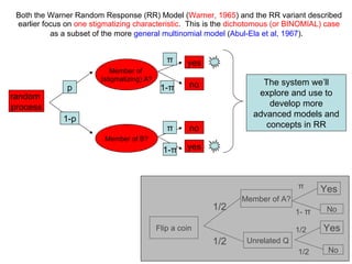
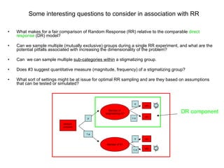
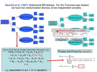
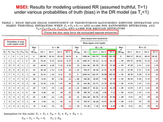
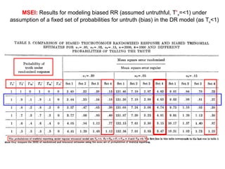
This document discusses simulations of multinomial randomized response models. It describes how the Warner randomized response model was extended to allow for multiple mutually exclusive categories. The key points are: 1) Abul-Ela et al. (1967) defined the multinomial randomized response model which allows sampling of multiple groups during a single experiment. 2) Simulations of the trinomial randomized response model are discussed, including calculating variances, biases, and mean squared errors to compare to direct response models. 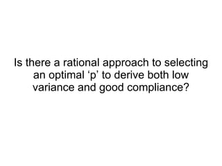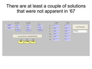3) Optimal values of the randomization probabilities (p-values) need to be determined to minimize variance while maximizing compliance for the trinomial model.

1. Simulations of Multinomial Randomized Response Models Tim Hare

2. Both the Warner Random Response (RR) Model ( Warner, 1965 ) and the RR variant described earlier focus on one stigmatizing characteristic . This is the dichotomous (or BINOMIAL) case as a subset of the more general multinomial model ( Abul-Ela et al, 1967 ). The system we’ll explore and use to develop more advanced models and concepts in RR Member of (stigmatizing) A? Member of B? random process no yes no yes 1-p p π 1- π π 1- π 1/2 1/2 1- π No No Yes Member of A? 1/2 Unrelated Q Flip a coin 1/2 π Yes

3. Some interesting questions to consider in association with RR What makes for a fair comparison of Random Response (RR) relative to the comparable direct response (DR) model? Can we sample multiple (mutually exclusive) groups during a single RR experiment, and what are the potential pitfalls associated with increasing the dimensionality of the problem? Can we can sample multiple sub-categories within a stigmatizing group. Does #3 suggest quantitative measure (magnitude, frequency) of a stigmatizing group? What sort of settings might be at issue for optimal RR sampling and are they based on assumptions that can be tested or simulated? DR component Member of (stigmatizing) A? Member of B? random process no yes no yes 1-p p π 1- π π 1- π

4. How do we measure the cost of using a RR approach ?

5. Partitioning of the overall RR model variance shows how it has the potential to be less precise relative to DR. RR variance = (sampling variance) + (random device variance) Sampling VAR RR device VAR + RR device VAR is function of ‘p’ & choice of ‘p’ not obvious Member of (stigmatizing) A? Member of B? random process no yes no yes 1-p p π 1- π π 1- π

6. The likelihood function (L, or L(x1,x2,…xn | p) can (aside from deriving our estimators) help understand RR variance concerns as function of ‘p’ MLE (log  Der  set0  solve for π )  RR estimators for π “ yes” “ no” “ yes” “ no” P=1/2 undefined Member of (stigmatizing) A? Member of B? random process no yes no yes 1-p p π 1- π π 1- π L(p): See Example Ex 9.6, Ex91.4 Wackerly, 7th Sample of random variables whose distribution depends on some parameter, p, then the likelihood L(x 1 , x 2 ,….x n | p) is the JOINT probability (e.g AND, e.g. multiply) of x 1 , x 2 , ….x n . Bernoulli: Xi = 0,1. Pr(Xi=xi)=p xi (1-p) 1-xi Likelihood (L, or L(p)) of the sample L(x 1  x n |p) = joint probabilty x 1  x n = П (p xi (1-p) (1-xi) =p Σ xi (1-p) n- Σ xi = p n1 (1-p) n-n1

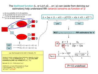
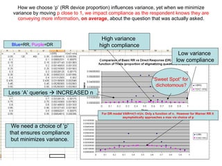
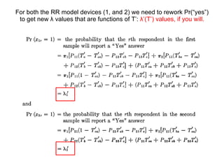
7. Likelihood (L) shows that VAR of the RR device & compliance (or truth) diametrically opposed as a function of ‘p’ . L(p, π ) = [ π p+(1- π )(1-p)] n1 [(1- π )p+ π (1-p)] n-n1 L( p=1, π ) = [ π +(1- π )(1-1)] n1 [(1- π )+ π (1-1)] n-n1 L( π ) = [ π )] n1 [1- π ] n-n1 If p=1 : L(p, π )  L( π ), in effect it becomes a DR model where likelihood depends entirely on π , therefore respondent no longer anonymous. L(p, π ) = [ π p+(1- π )(1-p)] n1 [(1- π )p+ π (1-p)] n-n1 L( p=1/2, π ) = [ π /2+(1- π )(1-1/2)] n1 [(1- π )1/2+ π (1-1/2)] n-n1 L(p=1/2, π ) = [ π /2+1/2- π /2)] n1 [1/2- π /2+ π /2] n-n1 L( p )=(1/2) n1 (1/2) n-n1 If p=1/2 L( p=1/2, π )  L( p ) likelihood does not depend on π , only depends on p , therefore no information is imparted by the sampling operation: e.g. nothing learned . The closer we get to p=½ (in this model) the less we know and the higher our variance, and the closer we get to p=1, the lower our variance but the less anonymity & compliance will be achieved.

8. Is there a rational approach to selecting an optimal ‘p’ to derive both low variance and good compliance?

9. How we choose ‘p’ (RR device proportion) influences variance, yet when we minimize variance by moving p close to 1, we impact compliance as the respondent knows they are conveying more information , on average , about the question that was actually asked. We need a choice of ‘p’ that ensures compliance but minimizes variance. Blue =RR, Purple =DR For DR model VAR= π (1- π )/n. Only a function of n. However for Warner RR it asymptotically approaches a max via choice of p High variance high compliance Low variance low compliance Less ‘A’ queries  INCREASED n “ Sweet Spot” for dichotomous?

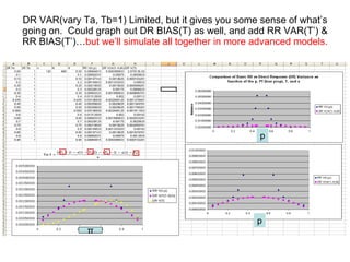
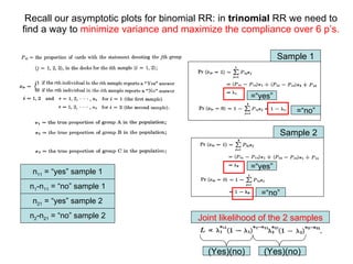
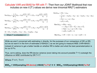
10. Let’s re-parameterize the DR model further by the inclusion of T , the probability of telling the truth . T will impact DR VAR and DR BIAS. So is the whole story represented by a low DR variance [V( π , n )] relative to RR (device, p) added variance [V( π , n, p )] ?

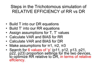
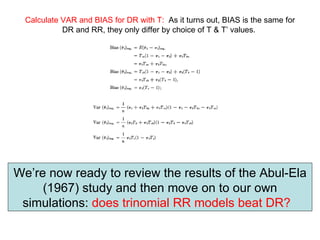
11. For a reasonable simulation w e need acknowledge known large magnitude DR BIAS, as well as additional variance based on compliance, as compared to the added RR device variance. T = probability of telling the truth, T (0  1), Ta=prob for group A, Tb=prob for group B 1) We can assume either that we have chosen a p that implies both Ta=Tb = 1 in the RR settings, that is, a ‘p’ that elicits the TRUTH , in that we will set p low enough to induce full cooperation in the RR setting. This works fine in dichotomous systems (e.g. “sweet spot”). 2) Or we can include estimates for Ta <1 and Tb <1 in either the DR model ( T ) and the RR model ( T ’ or “T prime”). In higher order systems this sort of simulation becomes more important. 3) Regarding assumptions for values of T or T ’ , what if we’re assessing ALCOHOL consumption magnitude or frequency? Might the direction of “stigmatizing” be less predictable and linked to social groupings? Might *both* the no-alcohol and “excessive alcohol” groups carry some stigma? Member of (stigmatizing) A? yes yes π Ta (1- π )(1- Tb ) a lie by B no no π (1- Ta ) (1- π )( Tb ) a lie by A Truth by A&B BIAS = π [ 1 - 1 -2]+[1- 1 ] = 0 , if truth VAR = [ π *1+(1- π )(1-1)][(1- π *1)-(1- π )(1-1)] = π *(1- π )/n under the assumption of truth (T=1), reduces to more familiar variance for X~Binomial( π ) as proportion E[ π ^] = π * 1 +[(1- π )(1- 1 ) = π , if truth Bias = E( π ^- π )=E( π ^) -E( π ) = E( π ^) - π = π (Ta)+1- π -Tb+ π (Tb)- π

12. DR VAR(vary Ta, Tb=1) Limited, but it gives you some sense of what’s going on. Could graph out DR BIAS(T) as well, and add RR VAR(T’) & RR BIAS(T’)… but we’ll simulate all together in more advanced models. π p p

13. The power of multinomial approaches comes into play when one assigns membership in sub-groups within a stigmatizing group C = ‘Use drugs 4+ times per week?’ B = ‘Use drugs 1-3 times per week?’ A = ‘Use drugs 0 times per week?’ - Historical impact - Abul-Ela (1967) extension of Warner(1965) model “propelled other authors to consider the RR technique for quantitative responses.” (Kim and Warde (2005).

14. Abul-Ela et al. (1967): Multinomial RR defined. For the Trinomial case (below) we have t wo randomization devices, & two independent samples. Pr(X 1r =1)=p 11 π 1 + p 12 π 2 + p 13 ( π 3 ) = p 11 π 1 + p 12 π 2 + p 13 ( 1- π 1 - π 2 ) = p 11 π 1 + p 12 π 2 + p 13 - p 13 π 1 -p 13 π 2 = (p 11 - p 13 ) π 1 + (p 12 -p 13 ) π 2 + p 13 = λ 1 (r th respondent in our 1  n1 sample1) Derive Prob that rth sample respondent will report “yes” Pr(yes) and Pr(no) for sample1 Member of group A? Member of group B? random process2 no yes yes no Member of group C? yes no π 1 π 2 π 3 1- π 1 1- π 2 1- π 3 p 21 p 22 p 23 Member of group A? Member of group B? random process1 no yes yes no Member of group C? yes no π 1 π 2 π 3 1- π 1 1- π 2 1- π 3 p 11 p 12 p 13 Likelihood of sample 1 in JOINT (Yes)(no) (Yes)(no)

15. Recall our asymptotic plots for binomial RR: in trinomial RR we need to find a way to minimize variance and maximize the compliance over 6 p’s. Sample 1 Sample 2 =“yes” =“yes” =“no” =“no” n 11 = “yes” sample 1 n 1 -n 11 = “no” sample 1 n 21 = “yes” sample 2 n 2 -n 21 = “no” sample 2 Joint likelihood of the 2 samples (Yes)(no) (Yes)(no)

16. Steps in the Trichotomous simulation of RELATIVE EFFICIENCY of RR vs DR Build T into our DR equations Build T’ into our RR equations Assign assumptions for T, T’ values Calculate VAR and BIAS for RR Calculate VAR and BIAS for DR Make assumptions for π 1, π 2, π 3 Search for 6 values of ‘p’ (p11, p12, p13, p21, p22, p23) proportion settings for the two devices, to optimize RR relative to DR, in terms of relative effciency.

17. Modeling some assumptions for values of T(and T’) for DR and RR to make a more sophisticated model NOTE: C is now the most stigmatizing group, and B somewhat, and A = neutral. Also, a group’s total probability (unity) includes it’s tendency to misrepresent itself, as in, say, Tb+Tba = 1, where some B’s report as A’s. The authors simplify matters by assuming respondents don’t misreport to a more stigmatizing group in the DR setting.

18. For both the RR model devices (1, and 2) we need to rework Pr(“yes”) to get new λ values that are functions of T’: λ ’(T’) values, if you will.

19. Calculate VAR and BIAS for RR with T’: Then from our JOINT likelihood that now includes on new λ ’(T’) values we derive new trinomial RR(T’) estimators Where T’ is embedded in λ ’ While we aren’t concerned with estimating π directly, for the purposes of our comparison of DR vs RR, but we do want it in the form of estimates of BIAS( π i ^ ) as we are going to measure MSE (VAR+BIAS 2 ) instead of variance to get a better handle on whether RR is better and what the best parameterization is for our 6 P’s. Thus, we’re asking, does the RR-device variance (even taking into account possible T’<1) outweigh the influence on MSE contributed by DR T<1? Where T’<=1, T<=1 MSE RR = VAR(sampling, RR-device ) )+BIAS( T’a,T’b ) 2  MSE DR =VAR(sampling)+BIAS( Ta,Tb ) 2

20. Calculate VAR and BIAS for DR with T: As it turns out, BIAS is the same for DR and RR, they only differ by choice of T & T’ values. We’re now ready to review the results of the Abul-Ela (1967) study and then move on to our own simulations: does trinomial RR models beat DR?

21. For a trinomial simulation we want to search for the optimal set of 6 proportions (p11,p12,p13, p21,p22,p23) split between the 2 randomization devices (samples). We also need to address assumptions regarding the true population proportions ( π 1, π 2, π 3 ), and different T, and T’ assumptions, before we can test for impact on efficiency via relative MSE. n1 n2 True proportion assumptions tested by Abul-Ela et al in 1967 smaller MSE values will favor RR and values less than 1 indicate RR is better “rand”=RR “ reg”=DR 4 sets of P’s tested by Abul-Ela in 1967

22. MSEI: Results for modeling unbiased RR (assumed truthful, T=1) under various probabilities of truth (bias) in the DR model (as T x <1)

23. MSEI: Results for modeling biased RR (assumed untruthful, T ’ x =<1) under assumption of a fixed set of probabilities for untruth (bias) in the DR model (as T x <1)

24. There are at least a couple of solutions that were not apparent in ‘67

25. Code for Trinomial RR. Pg1 Private Sub CalcMSE_Click() Dim p11 As Double Dim p12 As Double Dim p13 As Double Dim p21 As Double Dim p22 As Double Dim p23 As Double p11 = Me.p11 p12 = Me.p12 p13 = 1 - p11 - p12 Me.p13 = p13 p21 = Me.p21 p22 = Me.p22 p23 = 1 - p21 - p22 Me.p23 = p23 Dim true_prop1 As Double Dim true_prop2 As Double Dim true_prop3 As Double true_prop1 = Me.trueprop1 true_prop2 = Me.trueprop2 true_prop3 = 1 - true_prop1 - true_prop2 Me.trueprop3 = true_prop3 Dim result_bias_trueprop1_REG As Double Dim result_bias_trueprop2_REG As Double Dim result_bias_trueprop3_REG As Double Dim result_bias_trueprop1_RAN As Double Dim result_bias_trueprop2_RAN As Double Dim result_bias_trueprop3_RAN As Double Dim result_k As Double Dim result_lambda1_prime As Double Dim result_lambda2_prime As Double Dim result_var_truprop1_ran As Double Dim result_var_truprop1_reg As Double Dim result_mse_rand_truprop1 As Double Dim result_mse_reg_truprop1 As Double

26. Code for Trinomial RR. Pg2 Dim eff As Double result_bias_trueprop1_REG = bias_trueprop1_REG(true_prop2, true_prop3, Me.Tca_reg, Me.Tba_reg) result_bias_trueprop2_REG = bias_trueprop2_REG(true_prop2, true_prop3, Me.Tcb_reg, Me.Tb_reg) result_bias_trueprop3_REG = bias_trueprop3_REG(true_prop3, Me.Tc_reg) result_bias_trueprop1_RAN = bias_trueprop1_RAN(true_prop2, true_prop3, Me.Tca_ran, Me.Tba_ran) result_bias_trueprop2_RAN = bias_trueprop2_RAN(true_prop2, true_prop3, Me.Tcb_ran, Me.Tb_ran) result_bias_trueprop3_RAN = bias_trueprop3_RAN(true_prop3, Me.Tc_ran) result_k = k(Me.p11, Me.p12, Me.p13, Me.p21, Me.p22, Me.p23) result_lambda1_prime = lambda1_prime(Me.p11, Me.p12, Me.p13, Me.trueprop1, Me.trueprop2, Me.Tca_ran, Me.Tcb_ran, Me.Tc_ran, Me.Tba_ran, Me.Tb_ran) result_lambda2_prime = lambda2_prime(Me.p21, Me.p22, Me.p23, Me.trueprop1, Me.trueprop2, Me.Tca_ran, Me.Tcb_ran, Me.Tc_ran, Me.Tba_ran, Me.Tb_ran) result_var_truprop1_ran = var_truprop1_ran(result_k, Me.p12, Me.p13, Me.p22, Me.p23, Me.n1, Me.n2, result_lambda1_prime, result_lambda2_prime) result_var_truprop1_reg = var_truprop1_reg(Me.n1, Me.n2, Me.trueprop1, Me.trueprop2, Me.Tba_reg, Me.Tca_reg) result_mse_rand_truprop1 = MSE(result_var_truprop1_ran, result_bias_trueprop1_RAN) result_mse_reg_truprop1 = MSE(result_var_truprop1_reg, result_bias_trueprop1_REG) eff = result_mse_rand_truprop1 / result_mse_reg_truprop1 Me.efficiency = Format(eff, &quot;#.##&quot;) End Sub Private Function bias_trueprop1_RAN(true_prop2, true_prop3, Tca_ran, Tba_ran) bias_trueprop1_RAN = (true_prop3 * Tca_ran) + (true_prop2 * Tba_ran) End Function Private Function bias_trueprop1_REG(true_prop2, true_prop3, Tca_reg, Tba_reg) bias_trueprop1_REG = (true_prop3 * Tca_reg) + (true_prop2 * Tba_reg) End Function Private Function bias_trueprop2_RAN(true_prop2, true_prop3, Tcb_ran, Tb_ran)

27. Code for Trinomial RR. Pg3 bias_trueprop2_RAN = (true_prop3 * Tcb_ran) + (true_prop2 * (Tb_ran - 1)) End Function Private Function bias_trueprop2_REG(true_prop2, true_prop3, Tcb_reg, Tb_reg) bias_trueprop2_REG = (true_prop3 * Tcb_reg) + (true_prop2 * (Tb_reg - 1)) End Function Private Function bias_trueprop3_RAN(true_prop3, Tc_ran) bias_trueprop3_RAN = true_prop3 * (Tc_ran - 1) End Function Private Function bias_trueprop3_REG(true_prop3, Tc_reg) bias_trueprop3_REG = true_prop3 * (Tc_reg - 1) End Function Private Function k(p11, p12, p13, p21, p22, p23) k = (p11 - p13) * (p22 - p23) - (p12 - p13) * (p21 - p23) End Function Private Function lambda1_prime(p11, p12, p13, true_prop1, true_prop2, Tca_ran, Tcb_ran, Tc_ran, Tba_ran, Tb_ran) lambda1_prime = _ true_prop1 * (p11 * (1 - Tca_ran) - p12 * Tcb_ran - p13 * Tc_ran) + _ true_prop2 * (p11 * (Tba_ran - Tca_ran) + p12 * (Tb_ran - Tcb_ran) - p13 * Tc_ran) _ + (p11 * Tca_ran + p12 * Tcb_ran + p13 * Tc_ran) End Function Private Function lambda2_prime(p21, p22, p23, true_prop1, true_prop2, Tca_ran, Tcb_ran, Tc_ran, Tba_ran, Tb_ran) lambda2_prime = _ true_prop1 * (p21 * (1 - Tca_ran) - p22 * Tcb_ran - p23 * Tc_ran) _ + true_prop2 * (p21 * (Tba_ran - Tca_ran) + p22 * (Tb_ran - Tcb_ran) - p23 * Tc_ran) _ + (p21 * Tca_ran + p22 * Tcb_ran + p23 * Tc_ran) End Function Private Function var_truprop1_ran(k, p12, p13, p22, p23, n1, n2, lambda1_prime, lambda2_prime) var_truprop1_ran = (1 / (k ^ 2)) * _ ( _ ((p22 - p23) ^ 2) * (lambda1_prime * (1 - lambda1_prime) / n1) _ + ((p12 - p13) ^ 2) * (lambda2_prime * (1 - lambda1_prime) / n2) _ ) End Function

28. Code for Trinomial RR. Pg4 Private Function var_truprop2_ran(k, p11, p13, p21, p23, n1, n2, lambda1_prime, lambda2_prime) var_truprop1_ran = (1 / (k ^ 2)) * _ ( _ ((p21 - p23) ^ 2) * (lambda1_prime * (1 - lambda1_prime) / n1) _ + ((p11 - p13) ^ 2) * (lambda2_prime * (1 - lambda1_prime) / n2) _ ) End Function Private Function var_truprop3_ran(k, p11, p12, p21, p22, n1, n2, lambda1_prime, lambda2_prime) var_truprop1_ran = (1 / (k ^ 2)) * _ ( _ ((p22 - p21) ^ 2) * (lambda1_prime * (1 - lambda1_prime) / n1) _ + ((p12 - p11) ^ 2) * (lambda2_prime * (1 - lambda1_prime) / n2) _ ) End Function Private Function var_truprop1_reg(n1, n2, true_prop1, true_prop2, Tba_reg, Tca_reg) Dim true_prop3 As Double true_prop3 = 1 - true_prop1 - true_prop2 Dim n As Double n = n1 + n2 var_truprop1_reg = (1 / n) * (true_prop1 + true_prop2 * Tba_reg + true_prop3 * Tca_reg) * (1 - true_prop1 - true_prop2 * Tba_reg - true_prop3 * Tca_reg) End Function Private Function var_truprop2_reg(n1, n2, true_prop1, true_prop2, Tb_reg, Tcb_reg) Dim true_prop3 As Double true_prop3 = 1 - true_prop1 - true_prop2 Dim n As Double n = n1 + n2 var_truprop1_reg = (1 / n) * (true_prop2 * Tb_reg + true_prop3 * Tcb_reg) * (1 - true_prop2 * Tb_reg - true_prop3 * Tcb_reg) End Function Private Function var_truprop3_reg(n1, n2, true_prop1, true_prop2, Tc_reg) Dim true_prop3 As Double true_prop3 = 1 - true_prop1 - true_prop2 Dim n As Double n = n1 + n2 var_truprop1_reg = (1 / n) * (true_prop3 * Tc_reg) * (1 - true_prop3 * Tc_reg) End Function Private Function MSE(variance, bias) MSE = variance + bias ^ 2 End Function

29. The General Multinomial case

30. Assuming T=1 our DR model estimators for the trichotomous case are based on a standard multinomial distribution  Trinomial distribution PDF for trichotomous/trinomial DR is a subset of multinomial models P(x 1 x 2 ….x k ) = n! (p 1 x1 p 2 x1 … p k xk ) (x 1 ! x 2 ! …x k !) Multinomial Dist. Defn 5.12 Wackerly 7th The regular trinomial estimators resulting from a direct interviewing approach, say, where we draw a random sample of size n=n1+n2 (n independent trials) from a population consisting of three mutually exclusive groups with populations proportions π1, π2, π3 and every time a person is drawn from that sample they are asked to specify which group they below to (A,B, or C)

31. Generalization to the Multinomial Case Interest in estimating ‘t’ proportions leads to a likelihood involving t-1 samples

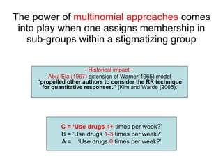
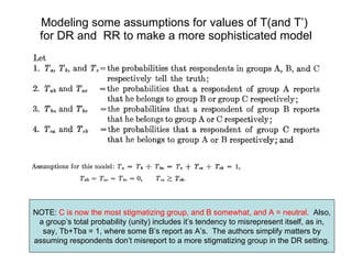
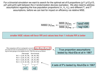
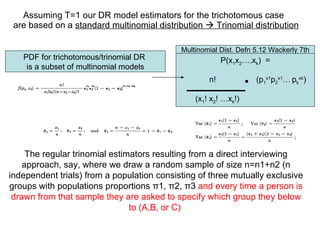
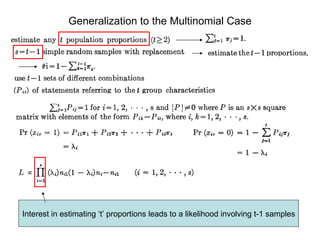
32. For the multinomial generalization one gets a s ystem of equations that show expectation and variance of the [ s x 1 ] vector of proportions ( π i )