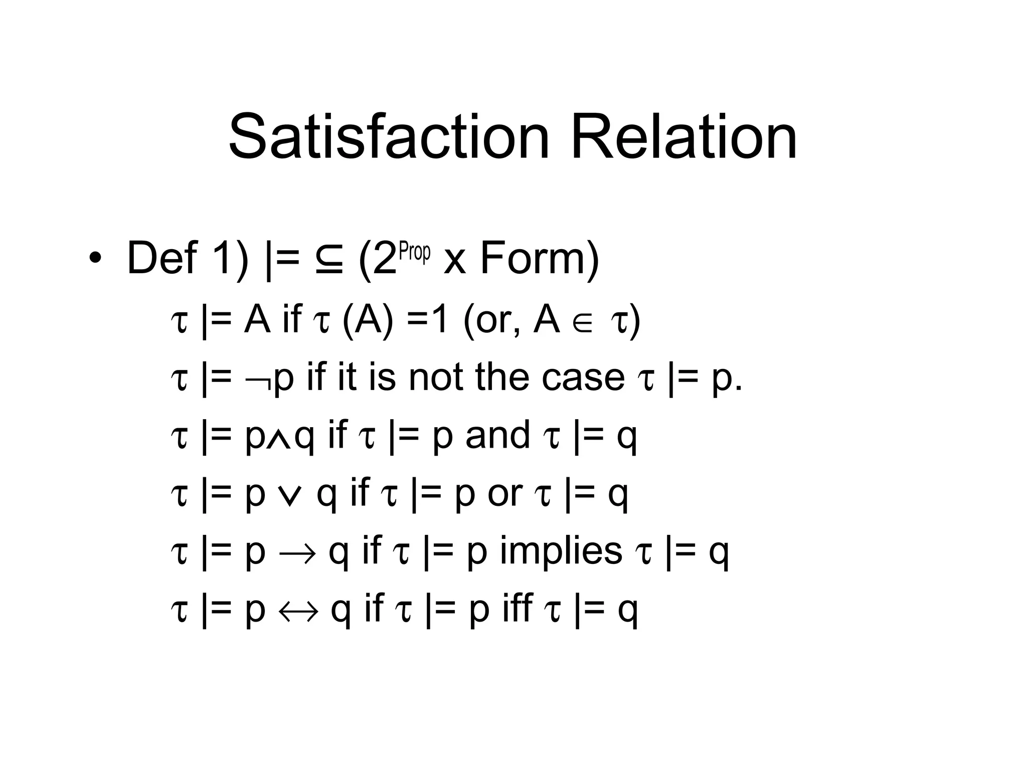
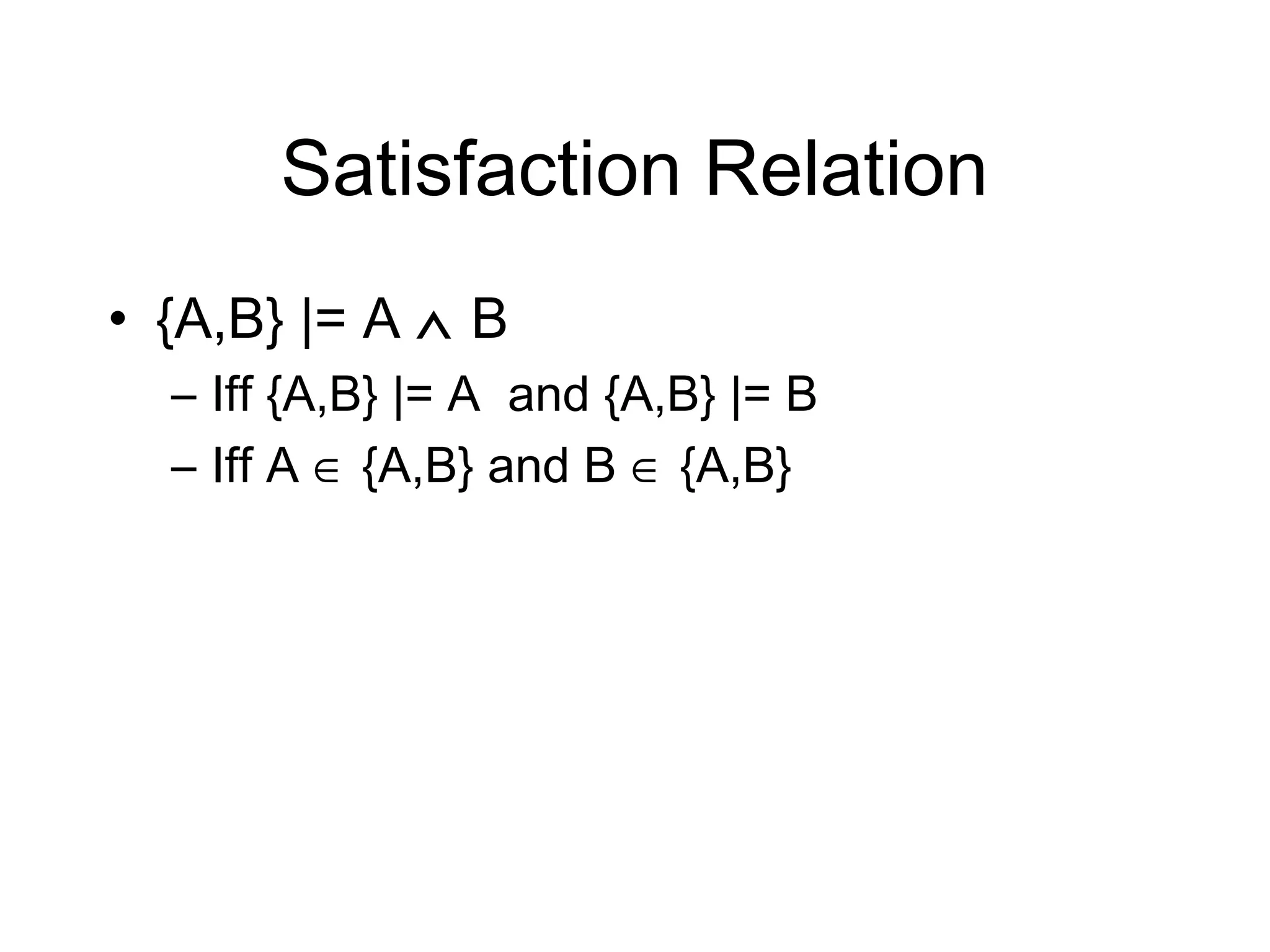
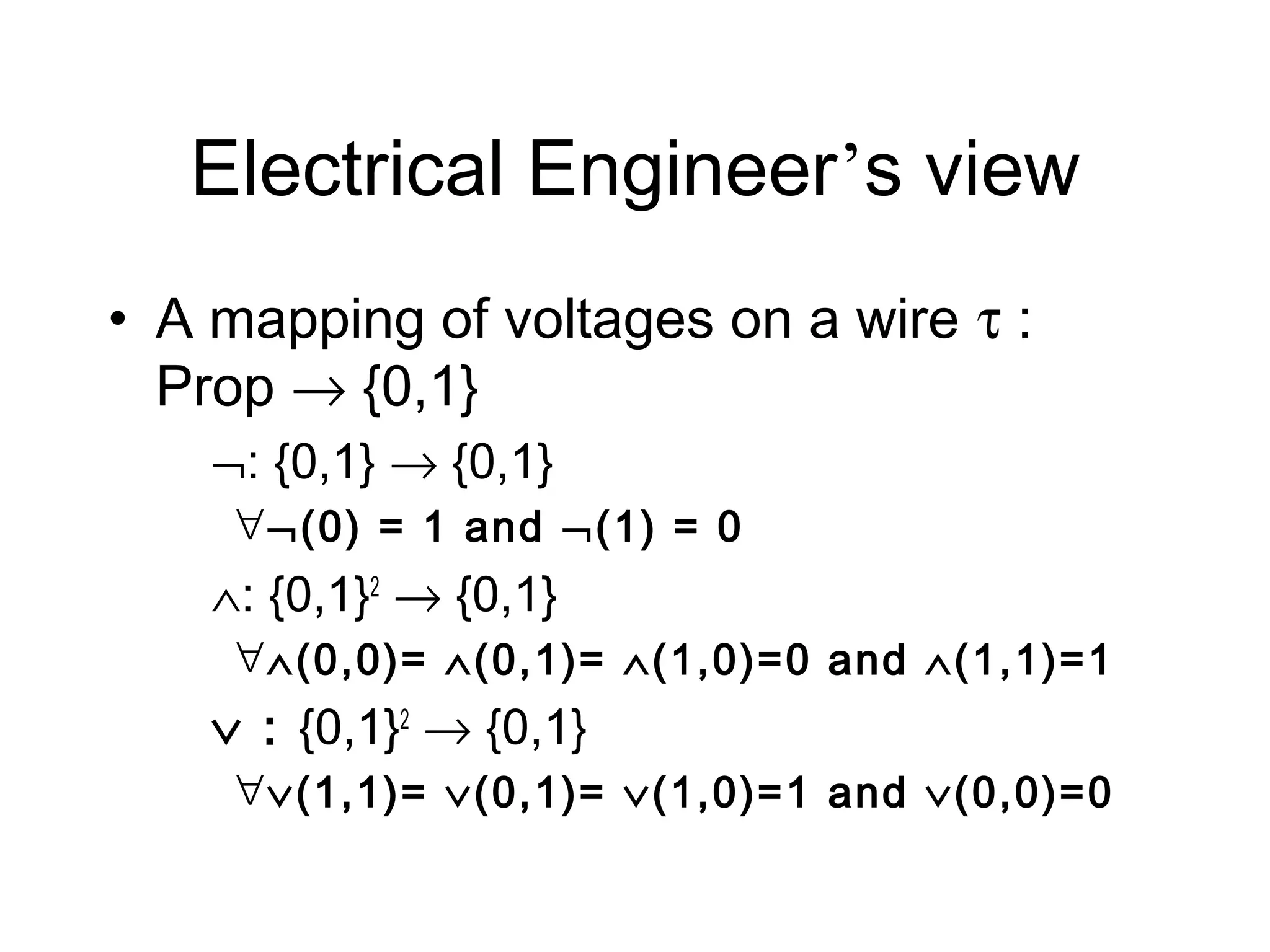
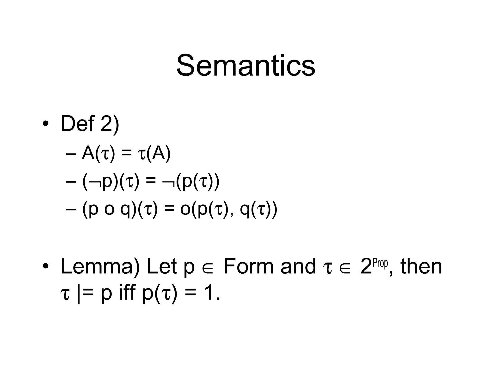
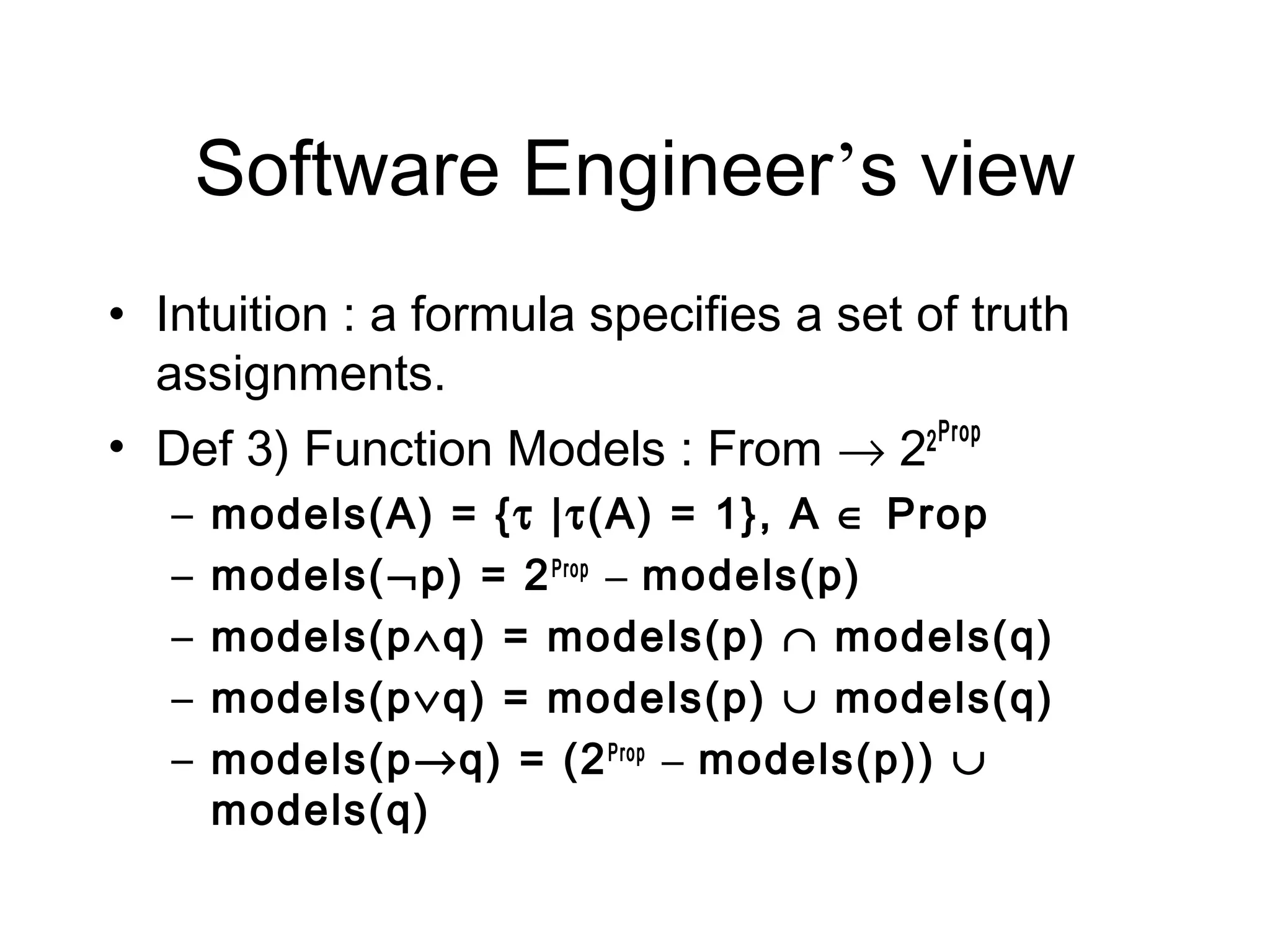
This document provides a brief introduction to logic by outlining its historical development and key concepts in propositional logic. It discusses how logic evolved from philosophical logic using natural languages to symbolic and mathematical logic using formal languages. It then defines propositional logic syntax using formulas and semantics using truth assignments. It explains how to determine if a truth assignment satisfies a formula and different perspectives on semantics. Finally, it introduces proofs in propositional logic using natural deduction rules.

1. Brief Introduction to Logic

2. Outline
• Historical View
• Propositional Logic : Syntax
• Propositional Logic : Semantics
• Satisfiability
• Natural Deduction : Proofs.

3. Historical view
• Philosophical Logic
– 500 BC to 19th Century
• Symbolic Logic
– Mid to late 19th Century
• Mathematical Logic
– Late 19th to mid 20th Century
• Logic in Computer Science

4. Philosophical Logic
• 500 B.C – 19th Century
• Logic dealt with arguments in the
natural language used by humans.
• Example
– All men are motal.
– Socrates is a man
– Therefore, Socrates is mortal.

5. Philosophical Logic
• Natural language is very ambiguous.
– Eric does not believe that Mary can pass any test.
– I only borrowed your car.
– Tom hates Jim and he likes Mary.
• It led to many paradoxes.
– “This sentence is a lie.” (The Liar’s Paradox)

6. The Sophist’s Paradox
• A Sophist is sued for his tuition by the
school that educated him. He argued
that he must win, since, if he loses, the
school didn’t educated him well
enough, and doesn’t deserve the
money. The school argue that he must
loss, since, if he win, he was educated
well enough therefore should pay for it.

7. Symbolic Logic
• Mid to late 19th Century.
• Attempted to formulate logic in terms of
a mathematical language
• Rules of inference were modeled after
various laws for manipulating algebraic
expressions.

8. Mathematical Logic
• Late 19th to mid 20th Century
• Frege proposed logic as a language for
mathematics in 1879.
• With the rigor of this new foundation, Cantor
was able to analyze the notion of infinity in
ways that were previously impossible. (2N is
strictly larger than N)
• Russell’s Paradox
T = { S | S ∉ S}

9. Logic in Computer Science
• In computer science, we design and
study systems through the use of formal
languages that can themselves be
interpreted by a formal system.
– Boolean circuits
– Programming languages
– Design Validation and verification
– AI, Security. Etc.

10. Logics in Computer Science
• Propositional Logic
• First Order Logic
• Higher Order Logic
• Theory of Construction
• Real-time Logic, Temporal Logic
• Process Algebras
• Linear Logic

11. Syntax
• The symbol of the language.
• Propositional symbols: A, B, C,…
• Prop: set of propositional symbols
• Connectives: ∧ (and), ∨ (or), ¬ (not), →
(implies), ↔ (is equivalent to), ⊥ (false).
• Parenthesis: (, ).

12. Formulas
• Backus-Naur Form
– Form := Prop | (¬Form) | (Form o Form).
• Context-Free Grammar
– Form → Prop,
– Form → (¬ Form),
– Form → (Form o Form)

13. Formulas (2)
• The set of formulas, Form, is defined as
the smallest set of expressions such
that:
1.Prop ⊆ Form
2.p∈Form⇒ (¬p)∈Form
3.p,q ∈Form ⇒ (p o q) ∈ Form

14. Formulas (3)
• Examples:
– (¬A)
– (¬(¬A))
– (A ∧ (B ∧ C))
– (A→ (B→ C))
– Correct expressions of Propositional Logic
are full of unnecessary parenthesis.

15. Formulas (4)
• Abbreviations . Let o=∧, ∨, →. We write
AoBoCo…
• in the place of
(A o (B o (C o …)))
• Thus, we write
A ∧ B ∧ C, A→B→C, …
• in the place of
(A ∧ (B ∧ C)), (A→ (B→ C))

16. Formulas (5)
• We omit parenthesis whenever we may
restore them through operator precedence:
∀ ¬ binds more strictly than ∧, ∨, and ∧, ∨ bind
more strictly than →, ↔.
• Thus, we write:
¬¬A for (¬(¬A)),
¬A ∧B for ((¬A ) ∧B)
A ∧B→ C for ((A∧B) → C), …

17. Semantics
• Def) A truth assignment, τ, is an
elements of 2Prop(I.e., τ ∈ 2Prop).
• Two ways to think of truth assignment
– 1) X ⊆ Prop
– 2) τ : Prop ↦ {0,1}
• Note : These notions are equivalence.

18. Philosopher’s view
• τ |= p means
τ satisfies p or
τ is true of p or
– p holds at τ or
τ is a model of p

19. Satisfaction Relation
• Def 1) |= ⊆ (2Prop x Form)
τ |= A if τ (A) =1 (or, A ∈ τ)
τ |= ¬p if it is not the case τ |= p.
τ |= p∧q if τ |= p and τ |= q
τ |= p ∨ q if τ |= p or τ |= q
τ |= p → q if τ |= p implies τ |= q
τ |= p ↔ q if τ |= p iff τ |= q

20. Satisfaction Relation
• {A,B} |= A ∧ B
– Iff {A,B} |= A and {A,B} |= B
– Iff A ∈ {A,B} and B ∈ {A,B}

21. Electrical Engineer’s view
• A mapping of voltages on a wire τ :
Prop → {0,1}
¬: {0,1} → {0,1}
∀ ¬(0) = 1 and ¬(1) = 0
∧: {0,1}2 → {0,1}
∀ ∧(0,0)= ∧(0,1)= ∧(1,0)=0 and ∧(1,1)=1
∨ : {0,1}2 → {0,1}
∀ ∨(1,1)= ∨(0,1)= ∨(1,0)=1 and ∨(0,0)=0

22. Semantics
• Def 2)
– A(τ) = τ(A)
– (¬p)(τ) = ¬(p(τ))
– (p o q)(τ) = o(p(τ), q(τ))
• Lemma) Let p ∈ Form and τ ∈ 2Prop, then
τ |= p iff p(τ) = 1.

23. Software Engineer’s view
• Intuition : a formula specifies a set of truth
assignments.
• Def 3) Function Models : From → 22 Prop
– models(A) = {τ |τ(A) = 1}, A ∈ Prop
– models(¬p) = 2 Prop – models(p)
– models(p∧q) = models(p) ∩ models(q)
– models(p∨q) = models(p) ∪ models(q)
– models(p→q) = (2 Prop – models(p)) ∪
models(q)

24. Theorem
• Let p ∈ Form and τ ∈ 2Prop, then the
following statements are all true:
– 1. τ |= p
– 2. p(τ) = 1
– 3. τ ∈ models(p)

25. Relevance Lemma
• Let’s use AP(p) to denote the set of all
propositional symbols occurred in p. Let
τ1, τ2 ∈ 2Prop, p∈Form.
• Lemma) if τ1|AP(p) = τ2|AP(p) , then
τ1|= p iff τ2 |= p
Corollary) τ| = p iff τ|AP(p) |= p

26. Algorithmic Perspective
• Truth Evaluation Problem
– Given p∈Form and τ ∈ 2AP(p), does τ |= p ?
Does p(τ) = 1 ?
• Eval(p, τ):
– If p ≡ A, return τ(A).
– If p ≡ (¬q), return ¬(Eval(q, τ))
– If p ≡ (q o r), return o(Eval(p), Eval(q))
• Eval uses polynomial time and space.

27. Extension of |=
• Let T ⊆ 2Prop, Γ ⊆ Form
• Def) T |= p if T ⊆ models(p)
– i.e., |= ⊆ 22Prop X Form
• Def) T |= Γ if T ⊆ models(Γ)
– models(Γ) = ∩p∈Γ models(p)
2Prop
– I.e., |= ⊆ 2 X 2Form

28. Extension of |=
• |= ⊆ 2Form x 2Form
• Def) Γ1 |= Γ2
iff models(Γ1) ⊆ models(Γ2)
Iff for all τ ∈ 2Prop
if τ |= Γ1 then τ |= Γ2

29. Semantic Classification
• A formula p is called valid if models(p) =
2Prop. We denote validity of the formula p
by |=p
• A formula p is called satisfiable if
models(p) ≠ ∅.
• A formula is not satisfiable is called
unsatisfiable or contradiction.

30. Semantic Classification(II)
• Lemma
– A formula p is valid iff ¬p is unsatifiable
– p is satisfiable iff ¬p is not valid
• Lemma
– p |= q iff |= (p → q)

31. Satisfiability Problem
• Given a p, is p satisfiable?
• SAT(p)
B:=0
for all τ ∈ 2 AP(p)
B = B ∨ Eval(p,τ)
end
return B
• NP-Complete

32. Proofs
• Formal Proofs. We introduce a notion of
formal proof of a formula p: Natural
Deduction.
• A formal proof of p is a tree whose root
is labeled p and whose children are
assumptions p1, p2, p3, … of the rule r we
used to conclude p.

33. Proofs
• Natural Deduction: Rules . For each
logical symbol o=⊥, ∧, ∨, →, and each
formula p with outermost connective o, we
give:
• A set of Introduction rules for o, describing
under which conditions p is true;
• A set of Elimination rules for o, describing
what we may infer from the truth of p.

34. Proofs
• Natural Deduction: notations for proofs.
• Let p be any formula, and Γ be a set of formulas.
We use the notation
Γ
…
p
• abbreviated by Γ|- p, for:
• “there is a proof of p whose assumptions are
included in Γ”.

35. Proofs
• Natural Deduction: assumptions of a proof
p1 p2 p3 …
r --------------------------------
p
• are inductively defined as:
• all assumptions of proofs of p1, p2, p3, …,
minus all assumptions we “crossed”.

36. Proofs
• Identity Principle: The simplest proof is:
p
-----
p
• having 1 assumption, p, and conclusion the
same p.
• We may express it by: Γ|-p, for all p∈Γ
• We call this proof “The Identity Principle”
(from p we derive p).

37. Proofs
• Rules for ⊥
• Introduction rules: none (⊥ is always
false).
• Elimination rules: from the truth of ⊥ (a
contradiction) we derive everything:
⊥
----
p
If Γ|- ⊥, then Γ|-p, for all p

38. Proofs
• Rules for ∧
• Introduction rules:
p q
--------
p∧q
• If Γ|- p and Γ|- q then Γ|- p ∧ q

39. Proofs
• Elimination rules:
p∧q p∧q
-------- -------
p q
• If Γ|- p ∧ q, then Γ|- p and Γ|- q

40. Proofs
• Rules for → Introduction rule:
[p]
…
q
--------
p→q
• If Γ,p |- q, then Γ|-p→q
• We may drop any number of assumptions equal to
p from the proof of q.

41. Proofs
• Elimination rule:
p→q p
----------------
q
• If Γ|-p→q and Γ|-p, then Γ |- q.

42. Proofs
• The only axiom not associated to a
connective, nor justified by some
Introduction rule, is Double Negation:
[¬p]
….
⊥
---
p
• If Γ, ¬p|- ⊥, then Γ|-p
• We may drop any number of assumptions equal to
¬p from the proof of q.

43. Soundness
|- p then |= p

44. Completeness
|= p then |- p