This document outlines the management of an experimental protocol using basic statistics to validate hypotheses, focusing on the budget and subject combinations necessary for significant results. It details the use of R for statistical simulations, creating various scenarios with healthy and sick subjects to determine the optimal combinations for detecting differences in means. Key findings suggest that a combination of 16 healthy and 36 sick patients maximizes detection probability within a budget of 10,000 euros.

1. How to manage your Experimental Protocol
with Basic Statistics
Y. Pageaud1
Friday, January 22, 2016
1 - Institute of Biology, Genetics and BioInformatics (IBGBI), 91000 Evry, France
Abstract:
The construction of an experimental protocol is the first step in any study to validate or invalidate a hypothesis
that we want to verify. Therefore, it is important to know how it will work in advance : how many subjects
do you want to include in the study, what budget is planned for the study, how to have significant results to
validate or invalidate you hypothesis. . . This document is an introduction to basic statistics to answer some
of these questions before starting your experimental protocol throught theoretical examples.
Data:
2 samples of healthy subjects and sick subjects were used for the examples to follow.
Material and Methods:
A computer (Packard Bell; Model imedia L4880; OS Win64 8.1/Linux; Processor Intel(R) Pentium(R) CPU
G3220 3.00 GHz; RAM 6.00 Go) was used. The softwares R and RStudio were installed. In RStudio, the
packages Rmarkdown and KnitR were downloaded and installed via the search bar in the tab “Packages”.
On the OS Windows, MiKTeX (Complete version) was installed. On the OS Linux, LaTeX was installed.
1

2. Protocol:
The budget was 10.000 euros. Each sick subjects were paid 100 euros for the experiment. Each healthy
subjects were paid 400 euros for the experiment. We needed to know how many sick and healthy subjects
will be taken to stay in our budget and to be statistically significant in our results.
Let n1 be the number of sick subjects. Let n2 be the number of healthy subjetcs. Let v1 be the vector that
will contain the different values of n1. Let v2 be the vector that will contain the different values of n2. A For
loop was built to calculate, for a budget of 10.000 euros, the possible combinations of sick-healthy subjects. 1
healthy subject cost as much as 4 sick subjects.
v1<-c()
v2<-c(2:24)
for (n2 in v2){
n1 <-100 - 4*n2
v1<-c(v1,n1)
}
Vectors were printed to see what they contain :
print(v1)
## [1] 92 88 84 80 76 72 68 64 60 56 52 48 44 40 36 32 28 24 20 16 12 8 4
print(v2)
## [1] 2 3 4 5 6 7 8 9 10 11 12 13 14 15 16 17 18 19 20 21 22 23 24
The values range from 2 to 24 for n2 :
• 2 is a minimum to apply a Student test (t-test)
• 24 is a maximum for healthy subjects because we need a minimum of 2 sick subjects to apply a Student
test.
2 Hypothesis were defined, H0 and H1:
• Let H0 be “the mean of expression of a gene is the same in sick and healthy subjects” : mean1=mean2
• Let H1 be “the mean of expression of a gene is different between sick and healthy subjects” :
mean1!=mean2
Means were arbitrarily set:
mean1=0
mean2=1
The alpha risk was set at 0.05 :
alpha = 0.05
2

3. 1st Example :
The function “population” was created.It allows us to apply a rnorm (random normalization) on healthy and
sick patients, and then to apply a student test. Finally, we checked if the p-value was less than alpha.
In this example the variance (V) was set at 1. in other term the standard deviation (sd) is also equal to 1 (V
= sd2) :
population=function(healthy,sick){
first<-rnorm(n = healthy, mean = mean1,sd=1)
second<-rnorm(n = sick, mean = mean2,sd=1)
res<-t.test(first,second)
res$p.value<alpha
}
• healthy is the number of healthy subjects.
• sick is the number of sick subjects.
The simulation “evo” was built:
We browse i from 2 to 24 healthy subjects with the number of sick subjects equals to 100 - 4*i.
5.000 simulations were done.
The probability of differentiating the two populations was calculated (calculations can sometimes take a few
minutes).
evo=rep(1,23)
for (i in 2:24){
res=rep(1,5000)
for (p in 1:5000){res[p]=population(healthy=i,sick= 100-4*i)}
evo[i-1]=mean(res)
}
We looked for a linear model that could fit as good as possible the data caculated. 2 vectors were created:
• v1: it contain the probabilities to differentiate the means of two populations healthy and sick
• v2: it contains the number of healthy patients
v1<- evo
v2<- c(2:24)
The vectors were stored in a list:
listv<-list(v1,v2)
The list was stored in a dataframe and each column were named respectively “Proba” “and”NbHealthy"
DF<-data.frame(listv)
colnames(DF) <- c("Proba","NbHealthy")
3

4. A linear model of type 3rd degree Polynomial Regression (PR) was used to be ajusted on the measures. it
inputs the formula of the linear model and the dataframe :
PR<-lm( Proba ~ NbHealthy + I(NbHealthy^2) + I(NbHealthy^3), data=DF)
A graph of the probability to differenciate 2 populations depending on the possible Sick-Healthy combinations
was plotted.
The PR model was superimposed to previous graph.Then, the equation of the model was retrieved :
plot (x = c(2:24),y=evo,type="p",col="blue",
xlab ="Number of Healthy Patients",
ylab="Probability of detection",
ylim = c(0,1),xlim = c(1,25),
main = "Evolution of the Probability of Detection of a difference n between the means of Healthy
par(new=TRUE)
plot(x = c(2:24), y=predict(PR),type = "l",lwd=3,col="red",
xlab ="",ylab="",
ylim = c(0,1),xlim = c(1,25),main = "")
5 10 15 20 25
0.00.20.40.60.81.0
Evolution of the Probability of Detection of a difference
between the means of Healthy and Sick patients
Number of Healthy Patients
Probabilityofdetection
5 10 15 20 25
0.00.20.40.60.81.0
4

5. PR
##
## Call:
## lm(formula = Proba ~ NbHealthy + I(NbHealthy^2) + I(NbHealthy^3),
## data = DF)
##
## Coefficients:
## (Intercept) NbHealthy I(NbHealthy^2) I(NbHealthy^3)
## 0.025992 0.073331 0.001550 -0.000161
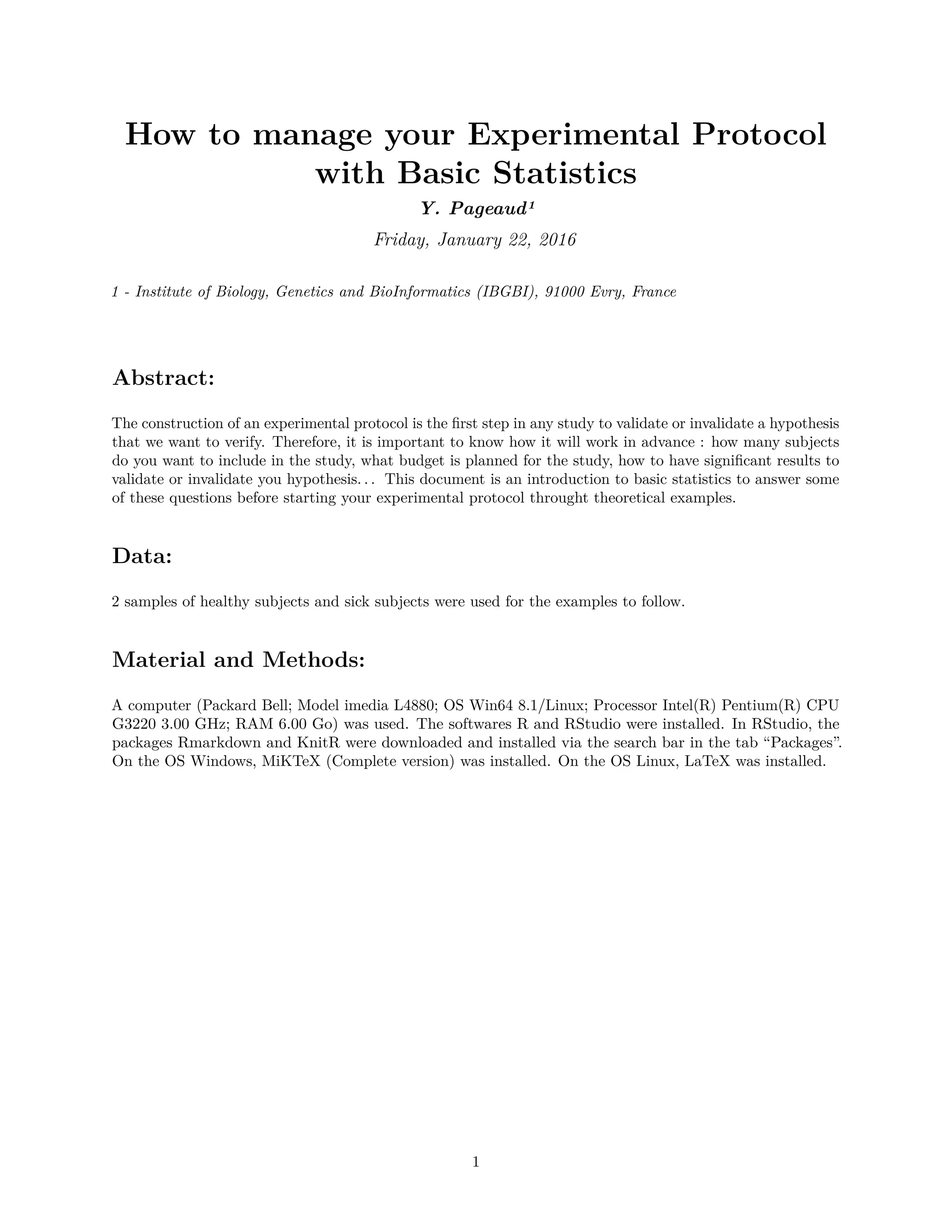
We can observe that the probability of detection of a difference increase with the number of Healthy patients
to reach a maximum between 16 and 17 Healthy patients, then it goes down because the number of Sick
patients becomes to low :
• If we follow the trend of the PR curve, the 16th combination (16 Healthy patients + 36 Sick patients)
gives the best probability.
• If we look at the highest point of measurement it is the 17th combination (17 Healthy patients + 32
Sick patients)
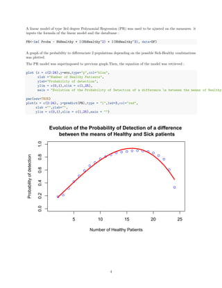
2nd Example :
In this example, we proceed as previously, but this time for 2 populations with means separated by 0.5 :
population=function(healthy,sick){
first<-rnorm(n = healthy,mean = 0,sd=1)
second<-rnorm(n = sick,mean = 0.5,sd=1)
res<-t.test(first,second)
res$p.value<0.05
}
evo=rep(1,23)
for (i in 2:24){
res=rep(0,5000)
for (p in 1:5000){res[p]=population(healthy=i,sick = 100-4*i)}
evo[i-1]=mean(res)
}
plot (x = c(2:24),y=evo,type="p",col="blue",
xlab ="Number of Healthy Patients",
ylab="Probability of detection",
ylim = c(0,0.5),xlim = c(1,25),
main = "Evolution of the Probability of Detection of a difference n between the means of Healthy
v1<- evo
v2<- c(2:24)
listv<-list(v1,v2)
DF<-data.frame(listv)
colnames(DF) <- c("Proba","NbHealthy")
5

6. PR<-lm( Proba ~ NbHealthy + I(NbHealthy^2) + I(NbHealthy^3), data=DF)
par(new=TRUE)
plot(x = c(2:24), y=predict(PR),type = "l",lwd=3,col="red",
xlab ="",ylab="",
ylim = c(0,0.5),xlim = c(1,25),main = "")
5 10 15 20 25
0.00.10.20.30.40.5
Evolution of the Probability of Detection of a difference
between the means of Healthy and Sick patients
Number of Healthy Patients
Probabilityofdetection
5 10 15 20 25
0.00.10.20.30.40.5
PR
##
## Call:
## lm(formula = Proba ~ NbHealthy + I(NbHealthy^2) + I(NbHealthy^3),
## data = DF)
##
## Coefficients:
## (Intercept) NbHealthy I(NbHealthy^2) I(NbHealthy^3)
## 0.1301233 -0.0108203 0.0038515 -0.0001403
The curve obtained confirm that the best Sick-Healthy patients combination is around 17 Healthy - 32 Sick
patients and 16 Healthy - 36 Sick patients.
6

7. 3rd Example :
In this 3rd example we are freed from the budget. The means of the 2 populations are fixed to be separated
by 1.
population=function(healthy,sick){
first<-rnorm(n = healthy,mean = 0,sd=1)
second<-rnorm(n = sick,mean = 1,sd=1)
res<-t.test(first,second)
res$p.value<0.05
}
The matrix evo was created it contains the probabilities to differentiate 2 populations :
• In column the number of healthy patients.
• In line the number of sick patients.
We decided to stop at 25 Healthy patients and 25 Sick patients because we already obtained a significant
probability of detection (as we will see later). lenMatrix was used to define the length of the matrix made. It
is a matrix of 25 lines and 25 columns. each column was named by the number of Healthy patients used for
the next simulations.
lenMatrix=25
evo=matrix(data = NA, nrow = lenMatrix, ncol = lenMatrix)
colnames(evo)=c("healthy1","healthy2","healthy3","healthy4","healthy5",
"healthy6","healthy7","healthy8","healthy9","healthy10",
"healthy11","healthy12","healthy13","healthy14","healthy15",
"healthy16","healthy17","healthy18","healthy19","healthy20",
"healthy21","healthy22","healthy23","healthy24","healthy25")
After that the matrix was created, we filled it. A first For loop was made with nbhealthy from 1 to 25. A
second For loop was made with nbsick from 1 to 25.
If a population (Healthy patients or Sick patients) has only 1 individual, we can not use the Student test,
and the function skip to the next iteration of a For loop.
For each combination Healthy-Sick, 1.000 simulations were done. Then, the probability of differentiation was
retrieved.
for (nbhealthy in 1:lenMatrix){
if (nbhealthy==1){next}
for (nbsick in 1:lenMatrix){
if (nbsick==1){next}
nbsimu=1000
res=rep(0,nbsimu)
for (simu in 1:nbsimu){res[simu]=population(healthy=nbhealthy,sick=nbsick)}
evo[nbsick,nbhealthy]=mean(res)
}
}
7

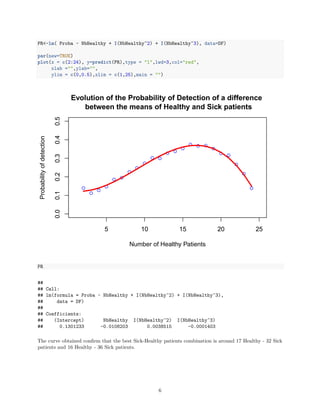
8. For 5, 10, 15 and 20 Healthy patients a graph of the probability to differenciate the means of the 2 populations
depending on the number of Sick patients was plotted.
Legends were added :
• topleft : topleft corner of the graph.
• inset : width between legends part and the side of the graph.
• fill : add colored squares.
matplot(evo[,c(5,10,15,20,25)],type="l",ylim = c(0,1),xlim=c(2,25),
main = "Evolution of the probability for 5, 10, 15, 20 and 25 Healthy patients n depending on t
xlab = "Number of Sick patients",
ylab= "Probability of Detection")
legend("topleft", inset = .01, title = "Legends",
legend= colnames(evo)[c(5,10,15,20,25)],fill = c(1:5))
5 10 15 20 25
0.00.20.40.60.81.0
Evolution of the probability for 5, 10, 15, 20 and 25 Healthy patients
depending on the number of Sick patients
Number of Sick patients
ProbabilityofDetection
Legends
healthy5
healthy10
healthy15
healthy20
healthy25
The probability of differentiation between the 2 means of the 2 populations is very low with 5 Healthy
whatever the number of Sick patients is.
This showed us that we need a minimum number of Healthy patients for the experiment.
8

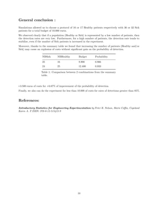
9. A summary table of the results for the 3rd example was made.
The table contained:
• The number of Sick patients
• The number of Healthy patients
• The budget for the experiment
• The probability associated with each Sick-Healthy combination
tab<-which(evo>0.85,arr.ind = T)
colnames(tab)=c("NBsick","NBhealthy")
budget=rep(1,length(tab[,1]))
proba=rep(1,length(tab[,1]))
for (i in 1:length(tab[,1])){
budget[i]=tab[i,1]*100+tab[i,2]*400
proba[i]=evo[tab[i,1],tab[i,2]]
}
head(cbind(tab,budget,proba),n = 10)
## NBsick NBhealthy budget proba
## [1,] 25 15 8500 0.860
## [2,] 23 16 8700 0.866
## [3,] 25 16 8900 0.859
## [4,] 23 17 9100 0.867
## [5,] 24 17 9200 0.870
## [6,] 25 17 9300 0.884
## [7,] 22 18 9400 0.878
## [8,] 23 18 9500 0.867
## [9,] 24 18 9600 0.880
## [10,] 25 18 9700 0.888
The head() function was only used to have a preview of the table.
9

10. General conclusion :
Simulations allowed us to choose a protocol of 16 or 17 Healthy patients respectively with 36 or 32 Sick
patients for a total budget of 10.000 euros.
We observed clearly that if a population (Healthy or Sick) is represented by a low number of patients, then
the detection rates are very low. Furthermore, for a high number of patients, the detection rate tends to
stabilize, even if the number of Sick patients is increased in the experiment.
Moreover, thanks to the summary table we found that increasing the number of patients (Healthy and/or
Sick) may cause an explosion of costs without significant gain on the probability of detection.
NBSick NBHealthy Budget Probability
25 16 8.900 0.866
24 25 12.400 0.933
Table 1: Comparison between 2 combinations from the summary
table.
+3.500 euros of costs for +6.67% of improvement of the probability of detection.
Finally, we also can do the experiment for less than 10.000 of costs for rates of detections greater than 85%.
References:
Introductory Statistics for Engineering Experimentation by Peter R. Nelson, Marie Coffin, Copeland
Karen A. F.ISBN: 978-0-12-515423-9
10