ALGORITHM EFFICIENCY WITH BIG O NOTATION

DEVELOPING EFFICIENT
ALGORITHMS
Objectives
■ To estimate algorithm efficiency using the Big O notation (§24.2).
■ To explain growth rates and why constants and nondominating terms can
be ignored in the estimation (§24.2).
■ To determine the complexity of various types of algorithms (§24.3).
■ To analyze the binary search algorithm (§24.4.1).
■ To analyze the selection sort algorithm (§24.4.2).
■ To analyze the insertion sort algorithm (§24.4.3).
■ To analyze the Towers of Hanoi algorithm (§24.4.4).
■ To describe common growth functions (constant, logarithmic, log-linear,
quadratic, cubic, exponential) (§24.4.5).
■ To design efficient algorithms for finding Fibonacci numbers using
dynamic programming (§24.5).
■ To find the GCD using Euclid’s algorithm (§24.6).
■ To find prime numbers using the sieve of Eratosthenes (§24.7).
■ To design efficient algorithms for finding the closest pair of points using
the divide-and-conquer approach (§24.8).
■ To solve the Eight Queens problem using the backtracking approach
(§24.9).
■ To design efficient algorithms for finding a convex hull for a set of points
(§24.10).
CHAPTER
24

854 Chapter 24 Developing Efficient Algorithms
24.1 Introduction
Algorithm design is to develop a mathematical process for solving a program.
Algorithm analysis is to predict the performance of an algorithm.
The preceding two chapters introduced classic data structures (lists, stacks, queues, priority
queues, sets, and maps) and applied them to solve problems. This chapter will use a variety of
examples to introduce common algorithmic techniques (dynamic programming, divide-and-
conquer, and backtracking) for developing efficient algorithms. Later in the book, we will
introduce efficient algorithms for trees and graphs in Chapters 27, 29, 30, and 31. Before
introducing developing efficient algorithms, we need to address the question on how to mea-
sure algorithm efficiency.
24.2 Measuring Algorithm Efficiency Using Big O
Notation
The Big O notation obtains a function for measuring algorithm time complexity based
on the input size. You can ignore multiplicative constants and nondominating terms in
the function.
Suppose two algorithms perform the same task, such as search (linear search vs. binary
search) or sort (selection sort vs. insertion sort). Which one is better? To answer this question,
you might implement these algorithms and run the programs to get execution time. But there
are two problems with this approach:
■ First, many tasks run concurrently on a computer. The execution time of a particular
program depends on the system load.
■ Second, the execution time depends on specific input. Consider, for example, linear
search and binary search. If an element to be searched happens to be the first in the
list, linear search will find the element quicker than binary search.
It is very difficult to compare algorithms by measuring their execution time. To overcome
these problems, a theoretical approach was developed to analyze algorithms independent of
computers and specific input. This approach approximates the effect of a change on the size
of the input. In this way, you can see how fast an algorithm’s execution time increases as the
input size increases, so you can compare two algorithms by examining their growth rates.
Consider linear search. The linear search algorithm compares the key with the elements
in the array sequentially until the key is found or the array is exhausted. If the key is not in
the array, it requires n comparisons for an array of size n. If the key is in the array, it
requires n/2 comparisons on average. The algorithm’s execution time is proportional to the
size of the array. If you double the size of the array, you will expect the number of compar-
isons to double. The algorithm grows at a linear rate. The growth rate has an order of mag-
nitude of n. Computer scientists use the Big O notation to represent the “order of
magnitude.” Using this notation, the complexity of the linear search algorithm is O(n), pro-
nounced as “order of n.”
For the same input size, an algorithm’s execution time may vary, depending on the input.
An input that results in the shortest execution time is called the best-case input, and an input
that results in the longest execution time is the worst-case input. Best-case analysis and worst-
case analysis are to analyze the algorithms for their best-case input and worst-case input.
Best-case and worst-case analysis are not representative, but worst-case analysis is very use-
ful. You can be assured that the algorithm will never be slower than the worst case. An
average-case analysis attempts to determine the average amount of time among all possible
inputs of the same size. Average-case analysis is ideal, but difficult to perform, because for
many problems it is hard to determine the relative probabilities and distributions of various
Key
Point
Key
Point
what is algorithm efficiency?
growth rates
Big O notation
best-case input
worst-case input
average-case analysis

24.2 Measuring Algorithm Efficiency Using Big O Notation 855
input instances. Worst-case analysis is easier to perform, so the analysis is generally con-
ducted for the worst case.
The linear search algorithm requires n comparisons in the worst case and n/2 comparisons
in the average case if you are nearly always looking for something known to be in the list.
Using the Big O notation, both cases require O(n) time. The multiplicative constant (1/2) can
be omitted. Algorithm analysis is focused on growth rate. The multiplicative constants have
no impact on growth rates. The growth rate for n/2 or 100n is the same as for n, as illustrated
in Table 24.1. Therefore,
Consider the algorithm for finding the maximum number in an array of n elements. To find
the maximum number if n is 2, it takes one comparison; if n is 3, two comparisons. In general,
it takes comparisons to find the maximum number in a list of n elements. Algorithm
analysis is for large input size. If the input size is small, there is no significance in estimating
an algorithm’s efficiency. As n grows larger, the n part in the expression dominates the
complexity. The Big O notation allows you to ignore the nondominating part (e.g., in the
expression ) and highlight the important part (e.g., n in the expression ). There-
fore, the complexity of this algorithm is O(n).
The Big O notation estimates the execution time of an algorithm in relation to the input
size. If the time is not related to the input size, the algorithm is said to take constant time with
the notation O(1). For example, a method that retrieves an element at a given index in an array
takes constant time, because the time does not grow as the size of the array increases.
The following mathematical summations are often useful in algorithm analysis:
24.1 Why is a constant factor ignored in the Big O notation? Why is a nondominating term
ignored in the Big O notation?
24.2 What is the order of each of the following functions?
(n2
+ 1)2
n
,
(n2
+ log2
n)2
n
, n3
+ 100n2
+ n, 2n
+ 100n2
+ 45n, n2n
+ n2
2n
20
+ 21
+ 22
+ 23
+ . . . . +˛2(n-1)
+ 2n
=
2n+1
- 1
2 - 1
= 2n+1
- 1 = O(2n
)
a0
+ a1
+ a2
+ a3
+ . . . . +˛a(n-1)
+ an
=
an+1
- 1
a - 1
= O(an
)
1 + 2 + 3 + . . . . +˛(n - 1) + n =
n(n + 1)
2
= O(n2
)
1 + 2 + 3 + . . . . +˛(n - 2) + (n - 1) =
n(n - 1)
2
= O(n2
)
n - 1n - 1
-˛1
n - 1
n - 1
O(n) = O(n/2) = O(100n).
ignoring multiplicative
constants
large input size
ignoring nondominating
terms
constant time
useful summations
✓Point✓Check
TABLE 24.1 Growth Rates
f(n)
n
n n/2 100n
100 100 50 10000
200 200 100 20000
2 2 2 f(200) / f(100)

Key
Point
24.3 Examples: Determining Big O
This section gives several examples of determining Big O for repetition, sequence, and
selection statements.
Example 1
Consider the time complexity for the following loop:
for (i = 1; i <= n; i++) {
k = k + 5;
}
It is a constant time, c, for executing
k = k + 5;
Since the loop is executed n times, the time complexity for the loop is
Example 2
What is the time complexity for the following loop?
for (i = 1; i <= n; i++) {
for (j = 1; j <= n; j++) {
k = k + i + j;
}
}
It is a constant time, c, for executing
k = k + i + j;
The outer loop executes n times. For each iteration in the outer loop, the inner loop is exe-
cuted n times. Thus, the time complexity for the loop is
An algorithm with the time complexity is called a quadratic algorithm. The quadratic
algorithm grows quickly as the problem size increases. If you double the input size, the time
for the algorithm is quadrupled. Algorithms with a nested loop are often quadratic.
Example 3
Consider the following loop:
for (i = 1; i <= n; i++) {
for (j = 1; j <= i; j++) {
k = k + i + j;
}
}
The outer loop executes n times. For the inner loop is executed one time, two
times, and n times. Thus, the time complexity for the loop is
= O(n2
)
= (c/2) n2
+ (c/2)n
= cn(n + 1)/2
T(n) = c + 2c + 3c + 4c + . . . + nc
i = 1, 2, . . . ,
O(n2
)
T(n) = (a constant c) * n * n = O(n2
)
T(n) = (a constant c) * n = O(n).
quadratic time

24.3 Examples: Determining Big O 857
Example 4
Consider the following loop:
for (i = 1; i <= n; i++) {
for (j = 1; j <= 20; j++) {
k = k + i + j;
}
}
The inner loop executes 20 times, and the outer loop n times. Therefore, the time complex-
ity for the loop is
Example 5
Consider the following sequences:
for (j = 1; j <= 10; j++) {
k = k + 4;
}
for (i = 1; i <= n; i++) {
for (j = 1; j <= 20; j++) {
k = k + i + j;
}
}
The first loop executes 10 times, and the second loop 20 * n times. Thus, the time complex-
ity for the loop is
Example 6
Consider the following selection statement:
if (list.contains(e)) {
System.out.println(e);
}
else
for (Object t: list) {
System.out.println(t);
}
Suppose the list contains n elements. The execution time for list.contains(e) is O(n).
The loop in the else clause takes O(n) time. Hence, the time complexity for the entire
statement is
Example 7
Consider the computation of for an integer n. A simple algorithm would multiply a n
times, as follows:
result = 1;
for (int i = 1; i <= n; i++)
result *= a;
an
= O(n) + O(n) = O(n)
T(n) = if test time + worst@case time(if clause, else clause)
T(n) = 10 * c + 20 * c * n = O(n)
T(n) = 20 * c * n = O(n)

✓Point✓Check
The algorithm takes O(n) time. Without loss of generality, assume You can improve
the algorithm using the following scheme:
result = a;
for (int i = 1; i <= k; i++)
result = result * result;
The algorithm takes O(logn) time. For an arbitrary n, you can revise the algorithm and prove
that the complexity is still O(logn). (See Checkpoint Question 24.7.)
Note
For simplicity, since 0(logn) 0(log2n) 0(logan), the constant base is omitted.
24.3 Count the number of iterations in the following loops.
==
n = 2k
.
omitting base
int count = 1;
while (count < 30) {
count = count * 2;
}
(a)
int count = 15;
while (count < 30) {
count = count * 3;
}
(b)
int count = 1;
while (count < n) {
count = count * 2;
}
(c)
int count = 15;
while (count < n) {
count = count * 3;
}
(d)
24.4 How many stars are displayed in the following code if n is 10? How many if n is 20?
Use the Big O notation to estimate the time complexity.
for (int i = 0; i < n; i++) {
System.out.print('*');
}
(a)
for (int i = 0; i < n; i++) {
for (int j = 0; j < n; j++) {
}
}
(b)
for (int k = 0; k < n; k++) {
for (int i = 0; i < n; i++) {
for (int j = 0; j < n; j++) {
}
}
}
(c)
for (int k = 0; k < 10; k++) {
for (int i = 0; i < n; i++) {
for (int j = 0; j < n; j++) {
}
}
}
(d)

24.4 Analyzing Algorithm Time Complexity 859
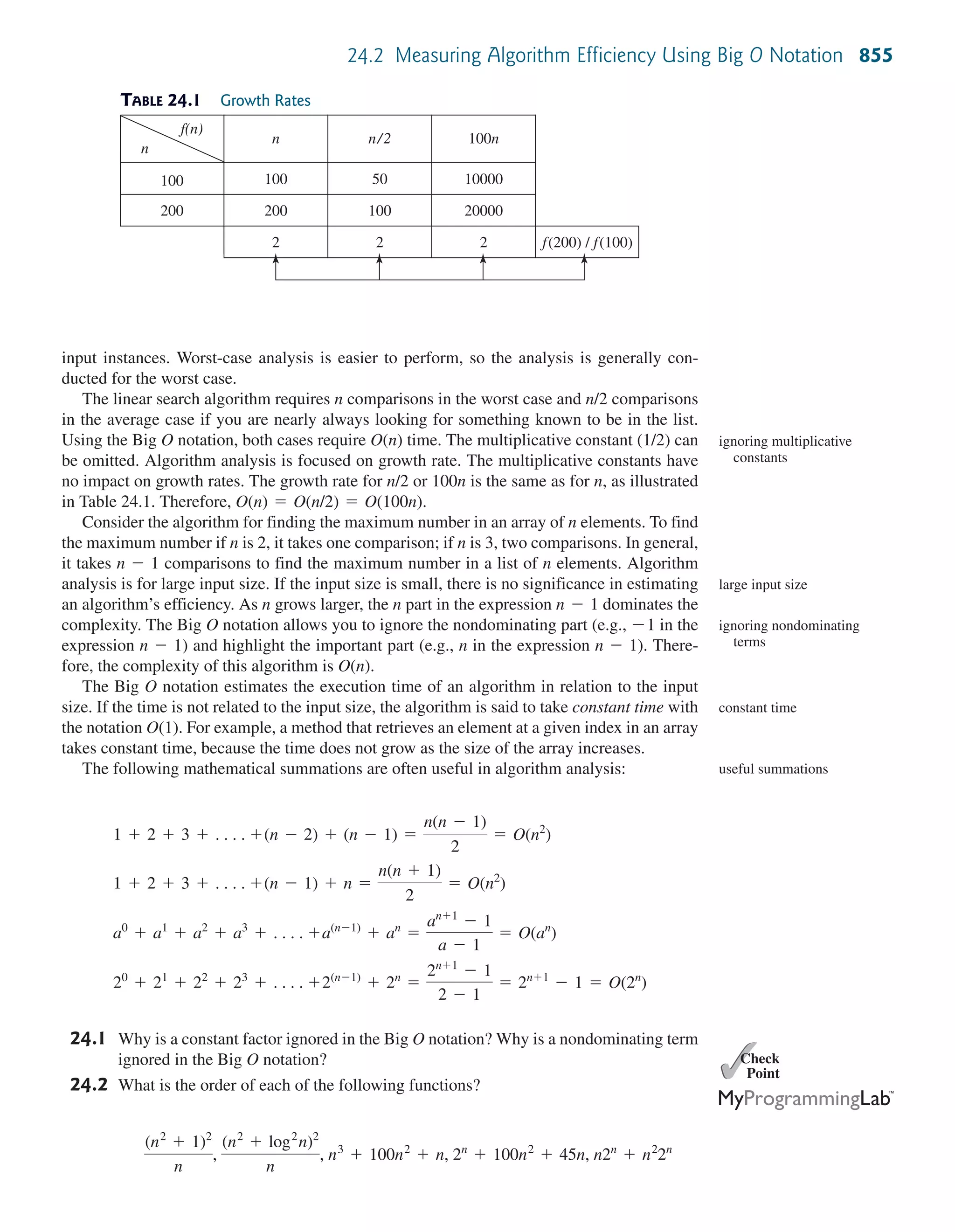
24.5 Use the Big O notation to estimate the time complexity of the following methods:
public static void mA(int n) {
for (int i = 0; i < n; i++) {
System.out.print(Math.random());
}
}
public static void mB(int n) {
for (int i = 0; i < n; i++) {
for (int j = 0; j < i; j++)
System.out.print(Math.random());
}
}
public static void mC(int[] m) {
for (int i = 0; i < m.length; i++) {
System.out.print(m[i]);
}
for (int i = m.length - 1; i >= 0; )
{
System.out.print(m[i]);
i--;
}
}
24.6 Design an O(n) time algorithm for computing the sum of numbers from n1 to n2 for
Can you design an O(1) for performing the same task?
24.7 Example 7 in Section 24.3 assumes Revise the algorithm for an arbitrary n
and prove that the complexity is still O(logn).
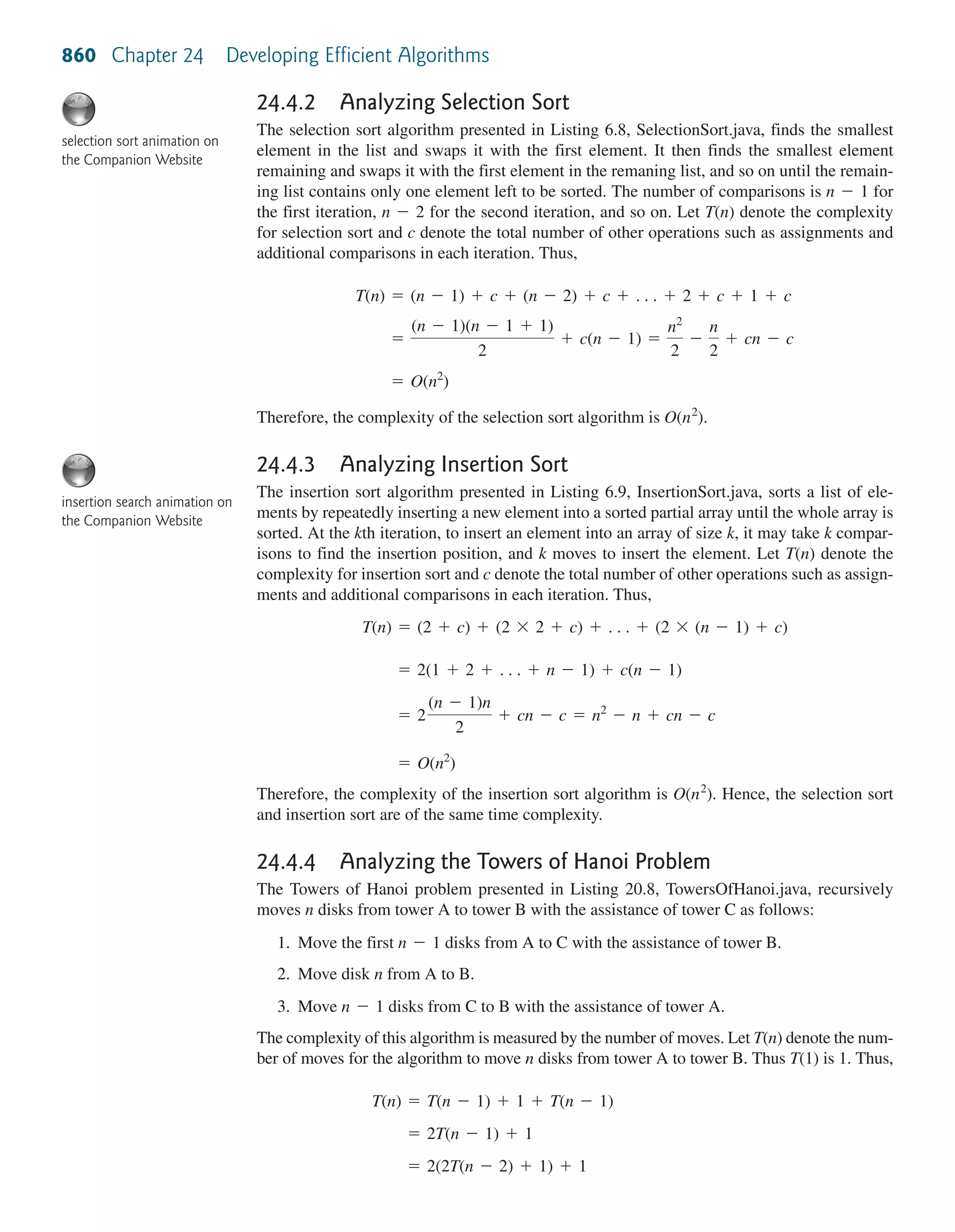
24.4 Analyzing Algorithm Time Complexity
This section analyzes the complexity of several well-known algorithms: binary search,
selection sort, insertion sort, and Towers of Hanoi.
24.4.1 Analyzing Binary Search
The binary search algorithm presented in Listing 6.7, BinarySearch.java, searches for a key in
a sorted array. Each iteration in the algorithm contains a fixed number of operations, denoted
by c. Let T(n) denote the time complexity for a binary search on a list of n elements. Without
loss of generality, assume n is a power of 2 and Since a binary search eliminates
half of the input after two comparisons,
Ignoring constants and nondominating terms, the complexity of the binary search algorithm is
O(logn). An algorithm with the O(logn) time complexity is called a logarithmic algorithm.
The base of the log is 2, but the base does not affect a logarithmic growth rate, so it can be
omitted. The logarithmic algorithm grows slowly as the problem size increases. In the case of
binary search, each time you double the array size, at most one more comparison will be
required. If you square the input size of any logarithmic time algorithm, you only double the
time of execution. So a logarithmic-time algorithm is very efficient.
= O(logn)
= T(1) + c logn = 1 + (logn)c
T(n) = T ¢
n
2
≤ + c = T ¢
n
22
≤ + c + c = T ¢
n
2k
≤ + kc
k = logn.
n = 2k
.
(n1 6 n2).
public static void mD(int[] m) {
for (int i = 0; i < m.length; i++) {
for (int j = 0; j < i; j++)
System.out.print(m[i] * m[j]);
}
}
Key
Point
binary search animation on
the Companion Website
logarithmic time
(a) (b)
(d)(c)

24.4.2 Analyzing Selection Sort
The selection sort algorithm presented in Listing 6.8, SelectionSort.java, finds the smallest
element in the list and swaps it with the first element. It then finds the smallest element
remaining and swaps it with the first element in the remaning list, and so on until the remain-
ing list contains only one element left to be sorted. The number of comparisons is for
the first iteration, for the second iteration, and so on. Let T(n) denote the complexity
for selection sort and c denote the total number of other operations such as assignments and
additional comparisons in each iteration. Thus,
Therefore, the complexity of the selection sort algorithm is
24.4.3 Analyzing Insertion Sort
The insertion sort algorithm presented in Listing 6.9, InsertionSort.java, sorts a list of ele-
ments by repeatedly inserting a new element into a sorted partial array until the whole array is
sorted. At the kth iteration, to insert an element into an array of size k, it may take k compar-
isons to find the insertion position, and k moves to insert the element. Let T(n) denote the
complexity for insertion sort and c denote the total number of other operations such as assign-
ments and additional comparisons in each iteration. Thus,
Therefore, the complexity of the insertion sort algorithm is Hence, the selection sort
and insertion sort are of the same time complexity.
24.4.4 Analyzing the Towers of Hanoi Problem
The Towers of Hanoi problem presented in Listing 20.8, TowersOfHanoi.java, recursively
moves n disks from tower A to tower B with the assistance of tower C as follows:
1. Move the first disks from A to C with the assistance of tower B.
2. Move disk n from A to B.
3. Move disks from C to B with the assistance of tower A.
The complexity of this algorithm is measured by the number of moves. Let T(n) denote the num-
ber of moves for the algorithm to move n disks from tower A to tower B. Thus T(1) is 1. Thus,
= 2(2T(n - 2) + 1) + 1
= 2T(n - 1) + 1
T(n) = T(n - 1) + 1 + T(n - 1)
n - 1
n - 1
O(n2
).
= O(n2
)
= 2
(n - 1)n
2
+ cn - c = n2
- n + cn - c
= 2(1 + 2 + . . . + n - 1) + c(n - 1)
T(n) = (2 + c) + (2 * 2 + c) + . . . + (2 * (n - 1) + c)
O(n2
).
= O(n2
)
=
(n - 1)(n - 1 + 1)
2
+ c(n - 1) =
n2
2
-
n
2
+ cn - c
T(n) = (n - 1) + c + (n - 2) + c + . . . + 2 + c + 1 + c
n - 2
n - 1
selection sort animation on
insertion search animation on

24.4 Analyzing Algorithm Time Complexity 861
An algorithm with time complexity is called an exponential algorithm. As the input
size increases, the time for the exponential algorithm grows exponentially. Exponential
algorithms are not practical for large input size. Suppose the disk is moved at a rate of 1 per
second. It would take years to move 32 disks and
billion years to move 64 disks.
24.4.5 Common Recurrence Relations
Recurrence relations are a useful tool for analyzing algorithm complexity. As shown in
the preceding examples, the complexity for binary search, selection sort and insertion
sort, and the Towers of Hanoi is and
respectively. Table 24.2 summarizes the common recurrence relations.2T(n - 1) + O(1),
T(n) =T(n) = T¢
n
2
≤ + c, T(n) = T(n - 1) + O(n),
264
/(365 * 24 * 60 * 60) = 585
232
/(365 * 24 * 60 * 60) = 136
O(2n
)
= 2n-1
+ 2n-2
+ . . . + 2 + 1 = (2n
- 1) = O(2n
)
= 2n-1
T(1) + 2n-2
+ . . . + 2 + 1
= 2(2(2T(n - 3) + 1) + 1) + 1
O(2n
)
exponential time
TABLE 24.2 Common Recurrence Functions
Recurrence Relation Result Example
T(n) = T(n/2) + O(1) T(n) = O(logn) Binary search, Euclid's GCD
T(n) = T(n - 1) + O(1) T(n) = O(n) Linear search
T(n) = 2T(n/2) + O(1) T(n) = O(n) Checkpoint Question 24.20
T(n) = 2T(n/2) + O(n) T(n) = O(n logn) Merge sort (Chapter 25)
T(n) = T(n - 1) + O(n) T(n) = O(n2
) Selection sort, insertion sort
T(n) = 2T(n - 1) + O(1) T(n) = O(2n
) Towers of Hanoi
T(n) = T(n - 1) + T(n - 2) + O(1) T(n) = O(2n
) Recursive Fibonacci algorithm
24.4.6 Comparing Common Growth Functions
The preceding sections analyzed the complexity of several algorithms. Table 24.3 lists some
common growth functions and shows how growth rates change as the input size doubles
from to n = 50.n = 25
TABLE 24.3 Change of Growth Rates
Function Name n = 25 n = 50 f(50)/f(25)
O(1) Constant time 1 1 1
O(logn) Logarithmic time 4.64 5.64 1.21
O(n) Linear time 25 50 2
O(n logn) Log-linear time 116 282 2.43
O(n2
) Quadratic time 625 2,500 4
O(n3
) Cubic time 15,625 125,000 8
O(2n
) Exponential time 3.36 * 107
1.27 * 1015
3.35 * 107

✓Point✓Check
Key
Point
O(1)
O(logn)
O(n)
O(nlogn)
O(2n
) O(n3
)
O(n2
)
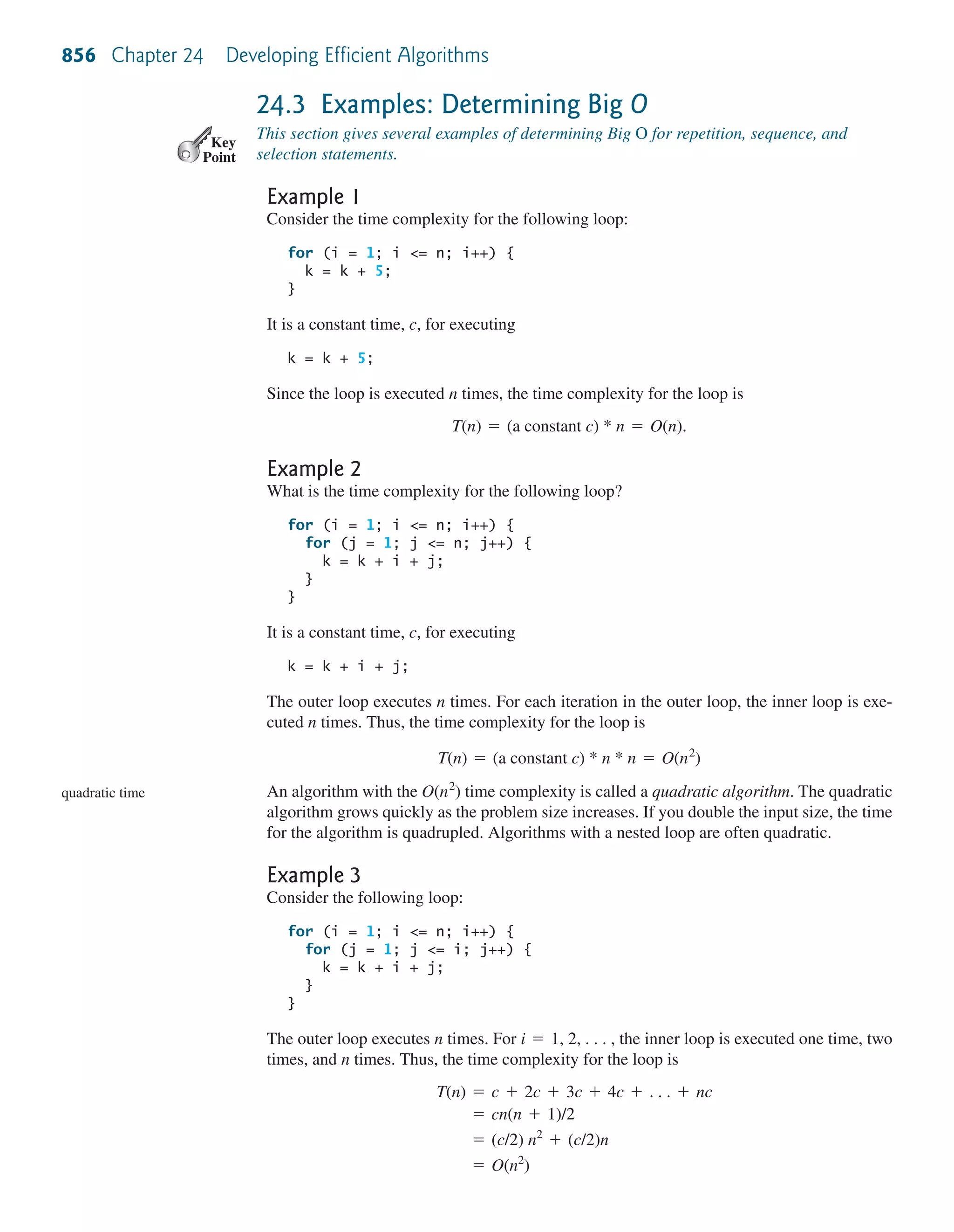
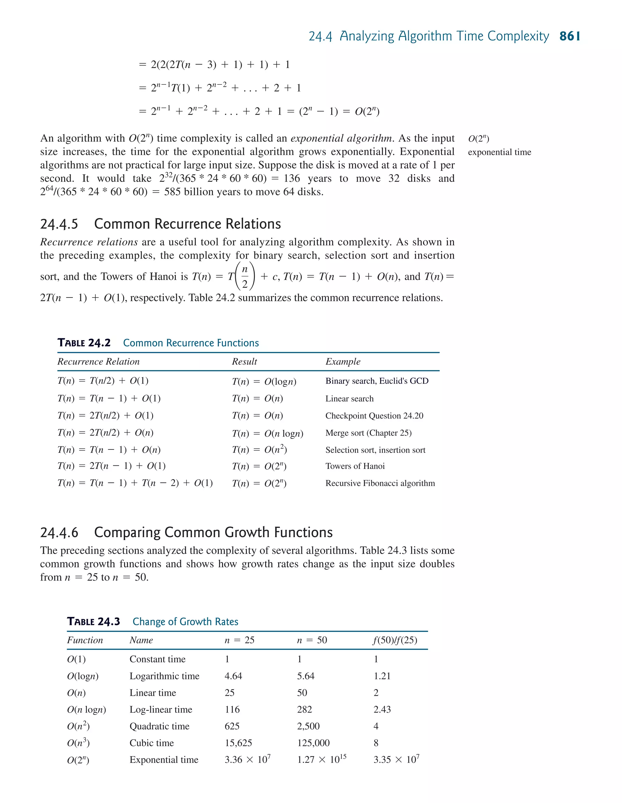
FIGURE 24.1 As the size n increases, the function grows.
These functions are ordered as follows, as illustrated in Figure 24.1.
O(1) 6 O(logn) 6 O(n) 6 O(n logn) 6 O(n2
) 6 O(n3
) 6 O(2n
)
24.8 Put the following growth functions in order:
24.9 Estimate the time complexity for adding two matrices, and for multiplying an
matrix by an matrix.
24.10 Describe an algorithm for finding the occurrence of the max element in an array.
Analyze the complexity of the algorithm.
24.11 Describe an algorithm for removing duplicates from an array. Analyze the complex-
ity of the algorithm.
24.12 Analyze the following sorting algorithm:
for (int i = 0; i < list.length - 1; i++) {
if (list[i] > list[i + 1]) {
swap list[i] with list[i + 1];
i = -1;
}
}
24.5 Finding Fibonacci Numbers Using Dynamic
Programming
This section analyzes and designs an efficient algorithm for finding Fibonacci numbers
using dynamic programming.
Section 20.3, Case Study: Computing Fibonacci Numbers, gave a recursive method for find-
ing the Fibonacci number, as follows:
/** The method for finding the Fibonacci number */
public static long {
if (index == 0) // Base case
return 0;
else if (index == 1) // Base case
return 1;
else // Reduction and recursive calls
return ;
}
fib(index - 1) + fib(index - 2)
fib(long index)
m * kn * m
n * m
5n3
4032
, 44 logn, 10n logn, 500, 2n2
,
2n
45
, 3n

24.5 Finding Fibonacci Numbers Using Dynamic Programming 863
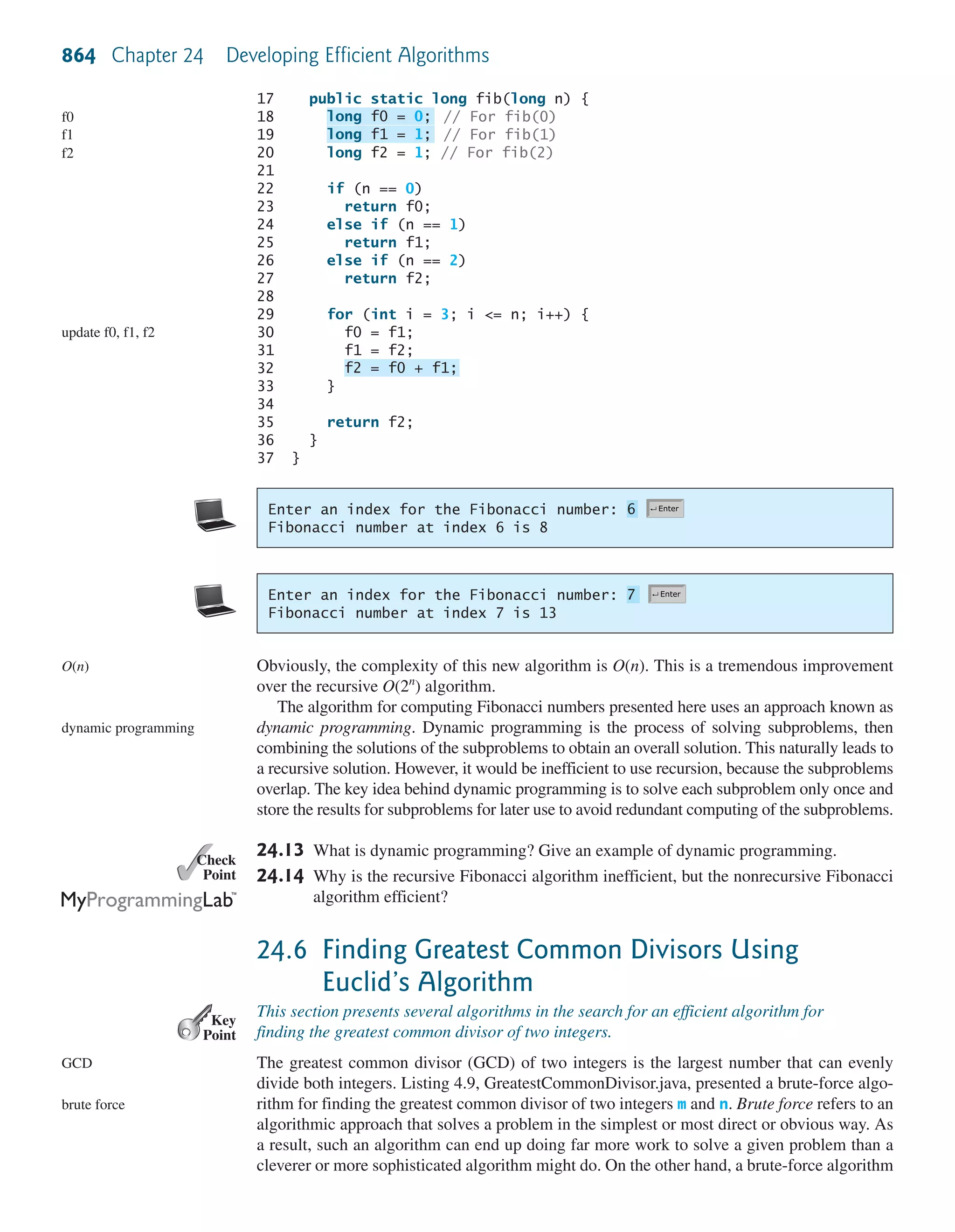
f0 f1 f2
Fibonacci series: 0 1 1 2 3 5 8 13 21 34 55 89 ...
indices: 0 1 2 3 4 5 6 7 8 9 10 11
f0 f1 f2
indices: 0 1 2 3 4 5 6 7 8 9 10 11
f0 f1 f2
indices: 0 1 2 3 4 5 6 7 8 9 10 11
We can now prove that the complexity of this algorithm is For convenience, let the
index be n. Let T(n) denote the complexity for the algorithm that finds fib(n) and c denote
the constant time for comparing the index with 0 and 1; that is, T(1) is c. Thus,
Similar to the analysis of the Towers of Hanoi problem, we can show that T(n) is
However, this algorithm is not efficient. Is there an efficient algorithm for finding a
Fibonacci number? The trouble with the recursive fib method is that the method is invoked
redundantly with the same arguments. For example, to compute fib(4), fib(3) and
fib(2) are invoked. To compute fib(3), fib(2) and fib(1) are invoked. Note that
fib(2) is redundantly invoked. We can improve it by avoiding repeated calling of the fib
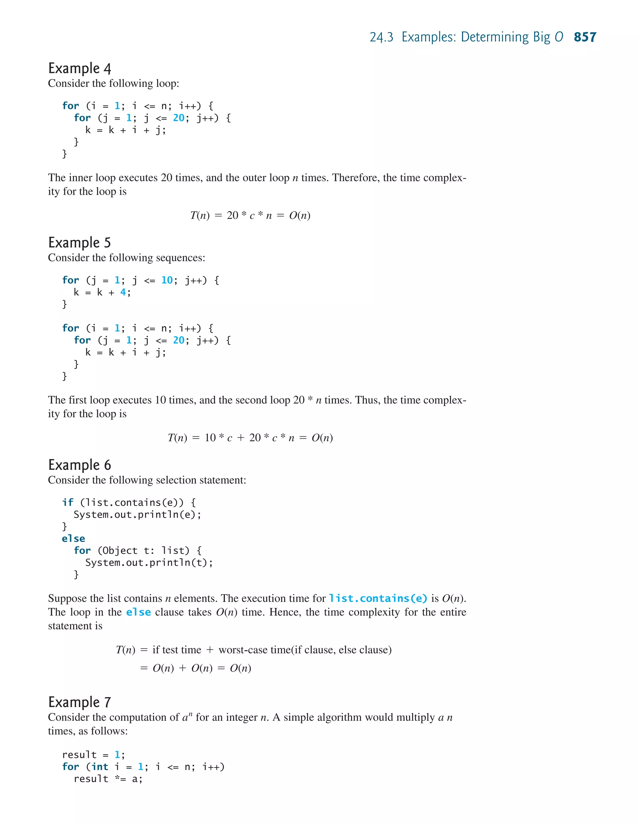
method with the same argument. Note that a new Fibonacci number is obtained by adding the
preceding two numbers in the sequence. If you use the two variables f0 and f1 to store the
two preceding numbers, the new number, f2, can be immediately obtained by adding f0 with
f1. Now you should update f0 and f1 by assigning f1 to f0 and assigning f2 to f1, as
shown in Figure 24.2.
O(2n
).
= 22
T(n - 2) + 2c + c
… 2(2T(n - 2) + c) + c
… 2T(n - 1) + c
T(n) = T(n - 1) + T(n - 2) + c
O(2n
).
The new method is implemented in Listing 24.1.
LISTING 24.1 ImprovedFibonacci.java
1 import java.util.Scanner;
2
3 public class ImprovedFibonacci {
4 /** Main method */
5 public static void main(String args[]) {
6 // Create a Scanner
7 Scanner input = new Scanner(System.in);
8 System.out.print("Enter an index for the Fibonacci number: ");
9
10
11 // Find and display the Fibonacci number
12 System.out.println(
13 "Fibonacci number at index " + index + " is " + );
14 }
15
16 /** The method for finding the Fibonacci number */
fib(index)
int index = input.nextInt(); input
invoke fib
FIGURE 24.2 Variables f0, f1, and f2 store three consecutive Fibonacci numbers in the series.

✓Point✓Check
Key
Point
17 public static long fib(long n) {
18 // For fib(0)
19 // For fib(1)
20 long f2 = 1; // For fib(2)
21
22 if (n == 0)
23 return f0;
24 else if (n == 1)
25 return f1;
26 else if (n == 2)
27 return f2;
28
29 for (int i = 3; i <= n; i++) {
30 f0 = f1;
31 f1 = f2;
32
33 }
34
35 return f2;
36 }
37 }
f2 = f0 + f1;
long f1 = 1;
long f0 = 0;f0
f1
f2
update f0, f1, f2
Enter an index for the Fibonacci number:
Fibonacci number at index 6 is 8
6
Enter an index for the Fibonacci number:
Fibonacci number at index 7 is 13
7
Obviously, the complexity of this new algorithm is O(n). This is a tremendous improvement
over the recursive algorithm.
The algorithm for computing Fibonacci numbers presented here uses an approach known as
dynamic programming. Dynamic programming is the process of solving subproblems, then
combining the solutions of the subproblems to obtain an overall solution. This naturally leads to
a recursive solution. However, it would be inefficient to use recursion, because the subproblems
overlap. The key idea behind dynamic programming is to solve each subproblem only once and
store the results for subproblems for later use to avoid redundant computing of the subproblems.
24.13 What is dynamic programming? Give an example of dynamic programming.
24.14 Why is the recursive Fibonacci algorithm inefficient, but the nonrecursive Fibonacci
algorithm efficient?
24.6 Finding Greatest Common Divisors Using
Euclid’s Algorithm
This section presents several algorithms in the search for an efficient algorithm for
finding the greatest common divisor of two integers.
The greatest common divisor (GCD) of two integers is the largest number that can evenly
divide both integers. Listing 4.9, GreatestCommonDivisor.java, presented a brute-force algo-
rithm for finding the greatest common divisor of two integers m and n. Brute force refers to an
algorithmic approach that solves a problem in the simplest or most direct or obvious way. As
a result, such an algorithm can end up doing far more work to solve a given problem than a
cleverer or more sophisticated algorithm might do. On the other hand, a brute-force algorithm
O(2n
)
O(n)
dynamic programming
GCD
brute force

24.6 Finding Greatest Common Divisors Using Euclid’s Algorithm 865
is often easier to implement than a more sophisticated one and, because of this simplicity,
sometimes it can be more efficient.
The brute-force algorithm checks whether k (for k = 2, 3, 4, and so on) is a common divisor
for n1 and n2, until k is greater than n1 or n2. The algorithm can be described as follows:
public static int gcd(int m, int n) {
int gcd = 1;
for (int k = 2; k <= m && k <= n; k++) {
if (m % k == 0 && n % k == 0)
gcd = k;
}
return gcd;
}
Assuming the complexity of this algorithm is obviously O(n).
Is there a better algorithm for finding the GCD? Rather than searching a possible divisor
from 1 up, it is more efficient to search from n down. Once a divisor is found, the divisor is
the GCD. Therefore, you can improve the algorithm using the following loop:
for (int k = n; k >= 1; k--) {
if (m % k == 0 && n % k == 0) {
gcd = k;
break;
}
}
This algorithm is better than the preceding one, but its worst-case time complexity is still O(n).
A divisor for a number n cannot be greater than n / 2, so you can further improve the
algorithm using the following loop:
for (int k = m / 2; k >= 1; k--) {
if (m % k == 0 && n % k == 0) {
gcd = k;
break;
}
}
However, this algorithm is incorrect, because n can be a divisor for m. This case must be con-
sidered. The correct algorithm is shown in Listing 24.2.
LISTING 24.2 GCD.java
2
3 public class GCD {
4 /** Find GCD for integers m and n */
5 public static int gcd(int m, int n) {
6 int gcd = 1;
7
8 if (m % n == 0) return n;
9
10 for (int k = n / 2; k >= 1; k--) {
11 if (m % k == 0 && n % k == 0) {
12 gcd = k;
13 break;
14 }
15 }
m Ն n, assume m Ն n
O(n)
improved solutions
check divisor
GCD found

16
17 return gcd;
18 }
19
21 public static void main(String[] args) {
24
25 // Prompt the user to enter two integers
26 System.out.print("Enter first integer: ");
27 int m = input.nextInt();
28 System.out.print("Enter second integer: ");
29 int n = input.nextInt();
30
31 System.out.println("The greatest common divisor for " + m +
32 " and " + n + " is " + gcd(m, n));
33 }
34 }
input
input
Enter first integer:
Enter second integer:
The greatest common divisor for 2525 and 125 is 25
125
2525
3
3
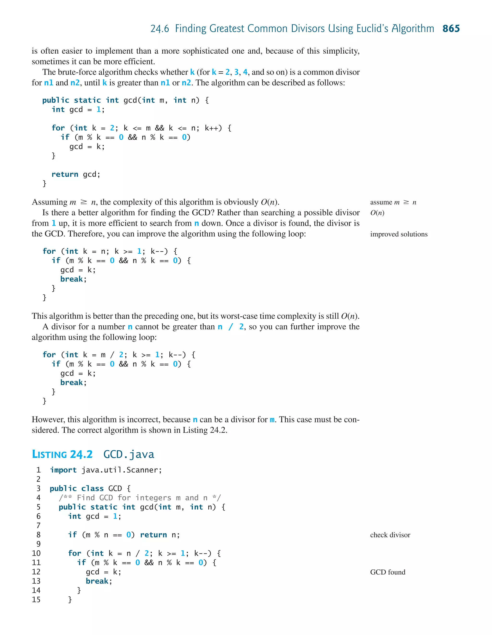
Assuming the for loop is executed at most n/2 times, which cuts the time by half
from the previous algorithm. The time complexity of this algorithm is still O(n), but practi-
cally, it is much faster than the algorithm in Listing 4.8.
Note
The Big O notation provides a good theoretical estimate of algorithm efficiency. How-
ever, two algorithms of the same time complexity are not necessarily equally efficient. As
shown in the preceding example, both algorithms in Listings 4.9 and 24.2 have the same
complexity, but in practice the one in Listing 24.2 is obviously better.
A more efficient algorithm for finding the GCD was discovered by Euclid around 300 B.C.
This is one of the oldest known algorithms. It can be defined recursively as follows:
Let gcd(m, n) denote the GCD for integers m and n:
■ If m % n is 0, gcd (m, n) is n.
■ Otherwise, gcd(m, n) is gcd(n, m % n).
It is not difficult to prove the correctness of this algorithm. Suppose m % n = r. Thus, m =
qn + r, where q is the quotient of m / n. Any number that is divisible by m and n must also
be divisible by r. Therefore, gcd(m, n) is the same as gcd(n, r), where r = m % n. The
algorithm can be implemented as in Listing 24.3.
LISTING 24.3 GCDEuclid.java
2
3 public class GCDEuclid {
m Ն n,
O(n)
practical consideration
Euclid’s algorithm

4 /** Find GCD for integers m and n */
5 public static int gcd(int m, int n) {
6 if (m % n == 0)
7 return n;
8 else
9 return gcd(n, m % n);
10 }
11
16
17 // Prompt the user to enter two integers
18 System.out.print("Enter first integer: ");
19 int m = input.nextInt();
20 System.out.print("Enter second integer: ");
22
23 System.out.println("The greatest common divisor for " + m +
24 " and " + n + " is " + gcd(m, n));
25 }
26 }
base case
reduction
input
input
125
2525
3
3
In the best case when m % n is 0, the algorithm takes just one step to find the GCD. It is dif-
ficult to analyze the average case. However, we can prove that the worst-case time complexity
is O(logn).
Assuming we can show that m % n < m / 2, as follows:
■ If n <= m / 2, m % n < m / 2, since the remainder of m divided by n is always
less than n.
■ If n > m / 2, m % n = m – n < m / 2. Therefore, m % n < m / 2.
Euclid’s algorithm recursively invokes the gcd method. It first calls gcd(m, n), then calls
gcd(n, m % n), and gcd(m % n, n % (m % n)), and so on, as follows:
gcd(m, n)
= gcd(n, m % n)
= gcd(m % n, n % (m % n))
= ...
Since m % n < m / 2 and n % (m % n) < n / 2, the argument passed to the gcd method
is reduced by half after every two iterations. After invoking gcd two times, the second para-
meter is less than n/2. After invoking gcd four times, the second parameter is less than n/4.
After invoking gcd six times, the second parameter is less than Let k be the number of
n
23
.
m Ն n,
best case
average case
worst case
24.6 Finding Greatest Common Divisors Using Euclid’s Algorithm 867

✓Point✓Check
TABLE 24.4 Comparisons of GCD Algorithms
Algorithm Complexity Description
Listing 4.9 O(n) Brute-force, checking all possible divisors
Listing 24.2 O(n) Checking half of all possible divisors
Listing 24.3 O(logn) Euclid's algorithm
times the gcd method is invoked. After invoking gcd k times, the second parameter is less
than which is greater than or equal to 1. That is,
Therefore, So the time complexity of the gcd method is O(logn).
The worst case occurs when the two numbers result in the most divisions. It turns out that
two successive Fibonacci numbers will result in the most divisions. Recall that the Fibonacci
series begins with 0 and 1, and each subsequent number is the sum of the preceding two num-
bers in the series, such as:
0 1 1 2 3 5 8 13 21 34 55 89 . . .
The series can be recursively defined as
fib(0) = 0;
fib(1) = 1;
fib(index) = fib(index - 2) + fib(index - 1); index >= 2
For two successive Fibonacci numbers fib(index) and fib(index - 1),
gcd(fib(index), fib(index - 1))
= gcd(fib(index - 1), fib(index - 2))
= ...
= gcd(fib(2), fib(1))
= 1
For example,
gcd(21, 13)
= gcd(13, 8)
= gcd(8, 5)
= gcd(5, 3)
= gcd(3, 2)
= gcd(2, 1)
= 1
Therefore, the number of times the gcd method is invoked is the same as the index. We can
prove that where This is a tighter bound than
Table 24.4 summarizes the complexity of three algorithms for finding the GCD.
index … 2 logn.
n = fib(index - 1).index … 1.44 logn,
k … 2 logn.
n
2(k/2)
Ն 1 = 7 n Ն 2(k/2)
= 7 logn Ն k/2 = 7 k … 2 logn
n
2(k/2)
,
24.15 Prove that the following algorithm for finding the GCD of the two integers m and n
is incorrect.
int gcd = 1;
for (int k = Math.min(Math.sqrt(n), Math.sqrt(m)); k >= 1; k--) {

24.7 Efficient Algorithms for Finding Prime Numbers 869
Key
Point
if (m % k == 0 && n % k == 0) {
gcd = k;
break;
}
}
24.7 Efficient Algorithms for Finding Prime Numbers
This section presents several algorithms in the search for an efficient algorithm for
finding prime numbers.
A $150,000 award awaits the first individual or group who discovers a prime number with at
least 100,000,000 decimal digits (w2.eff.org/awards/coop-prime-rules.php).
Can you design a fast algorithm for finding prime numbers?
An integer greater than 1 is prime if its only positive divisor is 1 or itself. For example, 2,
3, 5, and 7 are prime numbers, but 4, 6, 8, and 9 are not.
How do you determine whether a number n is prime? Listing 4.14 presented a brute-force
algorithm for finding prime numbers. The algorithm checks whether 2, 3, 4, 5, . . . , or n - 1
is divisible by n. If not, n is prime. This algorithm takes O(n) time to check whether n is
prime. Note that you need to check only whether 2, 3, 4, 5, . . . , and n/2 is divisible by n. If
not, n is prime. This algorithm is slightly improved, but it is still of O(n).
In fact, we can prove that if n is not a prime, n must have a factor that is greater than 1 and
less than or equal to Here is the proof. Since n is not a prime, there exist two numbers p
and q such that n pq with Note that p must be less than or equal
to Hence, you need to check only whether 2, 3, 4, 5, . . . , or is divisible by n. If not,
n is prime. This significantly reduces the time complexity of the algorithm to
Now consider the algorithm for finding all the prime numbers up to n. A straightforward
implementation is to check whether i is prime for i 2, 3, 4, . . . , n. The program is given
in Listing 24.4.
LISTING 24.4 PrimeNumbers.java
2
3 public class PrimeNumbers {
6 System.out.print("Find all prime numbers <= n, enter n: ");
8
9 final int NUMBER_PER_LINE = 10; // Display 10 per line
10 int count = 0; // Count the number of prime numbers
11 int number = 2; // A number to be tested for primeness
12
13 System.out.println("The prime numbers are:");
14
15 // Repeatedly find prime numbers
16
17 // Assume the number is prime
18 boolean isPrime = true; // Is the current number prime?
19
20 // Test if number is prime
21
22
23 if (number % divisor == 0) { // If true, number is not prime
24 isPrime = false; // Set isPrime to false
25 break; // Exit the for loop
divisor++) {
for (int divisor = 2; divisor <= (int)(Math.sqrt(number));
while (number <= n) {
=
O(2n).
2n2n.
n = 2n 2n.1 6 p … q.=
2n.
what is prime?
check prime

26 }
27 }
28
29 // Print the prime number and increase the count
30
31 // Increase the count
32
33 if (count % NUMBER_PER_LINE == 0) {
34 // Print the number and advance to the new line
35 System.out.printf("%7dn", number);
36 }
37 else
38 System.out.printf("%7d", number);
39 }
40
41 // Check if the next number is prime
42
43 }
44
45 System.out.println("n" + count +
46 " prime(s) less than or equal to " + n);
47 }
48 }
number++;
count++;
if (isPrime) {increase count
check next number
Find all prime numbers <= n, enter n:
The prime numbers are:
2 3 5 7 11 13 17 19 23 29
31 37 41 43 47 53 59 61 67 71
...
...
168 prime(s) less than or equal to 1000
1000
The program is not efficient if you have to compute Math.sqrt(number) for every iteration
of the for loop (line 21). A good compiler should evaluate Math.sqrt(number) only once
for the entire for loop. To ensure this happens, you can explicitly replace line 21 with the fol-
lowing two lines:
int = (int)(Math.sqrt(number));
for (int divisor = 2; divisor <= ; divisor++) {
In fact, there is no need to actually compute Math.sqrt(number) for every number. You
need look only for the perfect squares such as 4, 9, 16, 25, 36, 49, and so on. Note that for all
the numbers between 36 and 48, inclusively, their (int)(Math.sqrt(number)) is 6. With
this insight, you can replace the code in lines 16–26 with the following:
...
// Repeatedly find prime numbers
while (number <= n) {
// Assume the number is prime
boolean isPrime = true; // Is the current number prime?
// Test if number is prime
if (squareRoot * squareRoot < number) squareRoot++;
int squareRoot = 1;
squareRoot
squareRoot

for (int divisor = 2; divisor <= squareRoot; divisor++) {
if (number % divisor == 0) { // If true, number is not prime
isPrime = false; // Set isPrime to false
break; // Exit the for loop
}
}
...
Now we turn our attention to analyzing the complexity of this program. Since it takes
steps in the for loop (lines 21–27) to check whether number i is prime, the algorithm takes
steps to find all the prime numbers less than or equal to n.
Observe that
Therefore, the time complexity for this algorithm is
To determine whether i is prime, the algorithm checks whether 2, 3, 4, 5, . . . , and are
divisible by i. This algorithm can be further improved. In fact, you need to check only whether
the prime numbers from 2 to are possible divisors for i.
We can prove that if i is not prime, there must exist a prime number p such that and
Here is the proof. Assume that i is not prime; let p be the smallest factor of i. p must
be prime, otherwise, p has a factor k with k is also a factor of i, which contradicts
that p be the smallest factor of i. Therefore, if i is not prime, you can find a prime number
from 2 to that is divisible by i. This leads to a more efficient algorithm for finding all
prime numbers up to n, as shown in Listing 24.5.
LISTING 24.5 EfficientPrimeNumbers.java
2
3 public class EfficientPrimeNumbers {
8
9 // A list to hold prime numbers
10 java.util.List<Integer> list =
11 new java.util.ArrayList<Integer>();
12
13 final int NUMBER_PER_LINE = 10; // Display 10 per line
14 int count = 0; // Count the number of prime numbers
15 int number = 2; // A number to be tested for primeness
16 // Check whether number <= squareRoot
17
18 System.out.println("The prime numbers are n");
19
20 // Repeatedly find prime numbers
21 while (number <= n) {
22 // Assume the number is prime
23 boolean isPrime = true; // Is the current number prime?
24
25
26
27 // Test whether number is prime
28 for (int k = 0; k < list.size()
29 && list.get(k) <= squareRoot; k++) {
30 if (number % list.get(k) == 0) { // If true, not prime
if (squareRoot * squareRoot < number) squareRoot++;
int squareRoot = 1;
2i
2 … k 6 p.
p … q.
i = pq
2i
2i
O(n2n).
22 + 23 + 24 + . . . + 2n … n2n
22 + 23 + 24 + . . . + 2n
2i
check prime

31 isPrime = false; // Set isPrime to false
32 break; // Exit the for loop
33 }
34 }
35
36 // Print the prime number and increase the count
37 if (isPrime) {
38 count++; // Increase the count
39 list.add(number); // Add a new prime to the list
40 if (count % NUMBER_PER_LINE == 0) {
41 // Print the number and advance to the new line
42 System.out.println(number);
43 }
44 else
45 System.out.print(number + " ");
46 }
47
48 // Check whether the next number is prime
49 number++;
50 }
51
54 }
55 }
increase count
check next number
2 3 5 7 11 13 17 19 23 29
31 37 41 43 47 53 59 61 67 71
...
...
1000
Let (i) denote the number of prime numbers less than or equal to i. The primes under 20 are
2, 3, 5, 7, 11, 13, 17, and 19. Therefore, (2) is 1, (3) is 2, (6) is 3, and (20) is 8.
It has been proved that (i) is approximately (see primes.utm.edu/howmany.shtml).
For each number i, the algorithm checks whether a prime number less than or equal to
is divisible by i. The number of the prime numbers less than or equal to is
Thus, the complexity for finding all prime numbers up to n is
Since for and
222
log 2
+
223
log 3
+
224
log 4
+
225
log 5
+
226
log 6
+
227
log 7
+
228
log 8
+ . . . +
22n
logn
6
2n2n
logn
n Ն 16,i 6 n
2i
logi
6
2n
logn
222
log 2
+
223
log 3
+
224
log 4
+
225
log 5
+
226
log 6
+
227
log 7
+
228
log 8
+ . . . +
22n
logn
2i
log2i
=
22i
logi
2i
2i
i
logi
p
pppp
p

ϫ ϫ T T T T T T T T T T T T T T T T T T T T T T T T T Tinitial
0 1 2 3 4 5 6 7 8 9 10 11 12 13 14 15 16 17 18 19 20 21 22 23 24 25 26 27
k = 2
index
primes array
ϫ ϫ T T F T F T F T F T F T F T F T F T F T F T F T F T
k = 3 ϫ ϫ T T F T F T F F F T F T F F F T F T F F F T F T F F
k = 5 ϫ ϫ T T F T F T F F F T F T F F F T F T F F F T F F F F
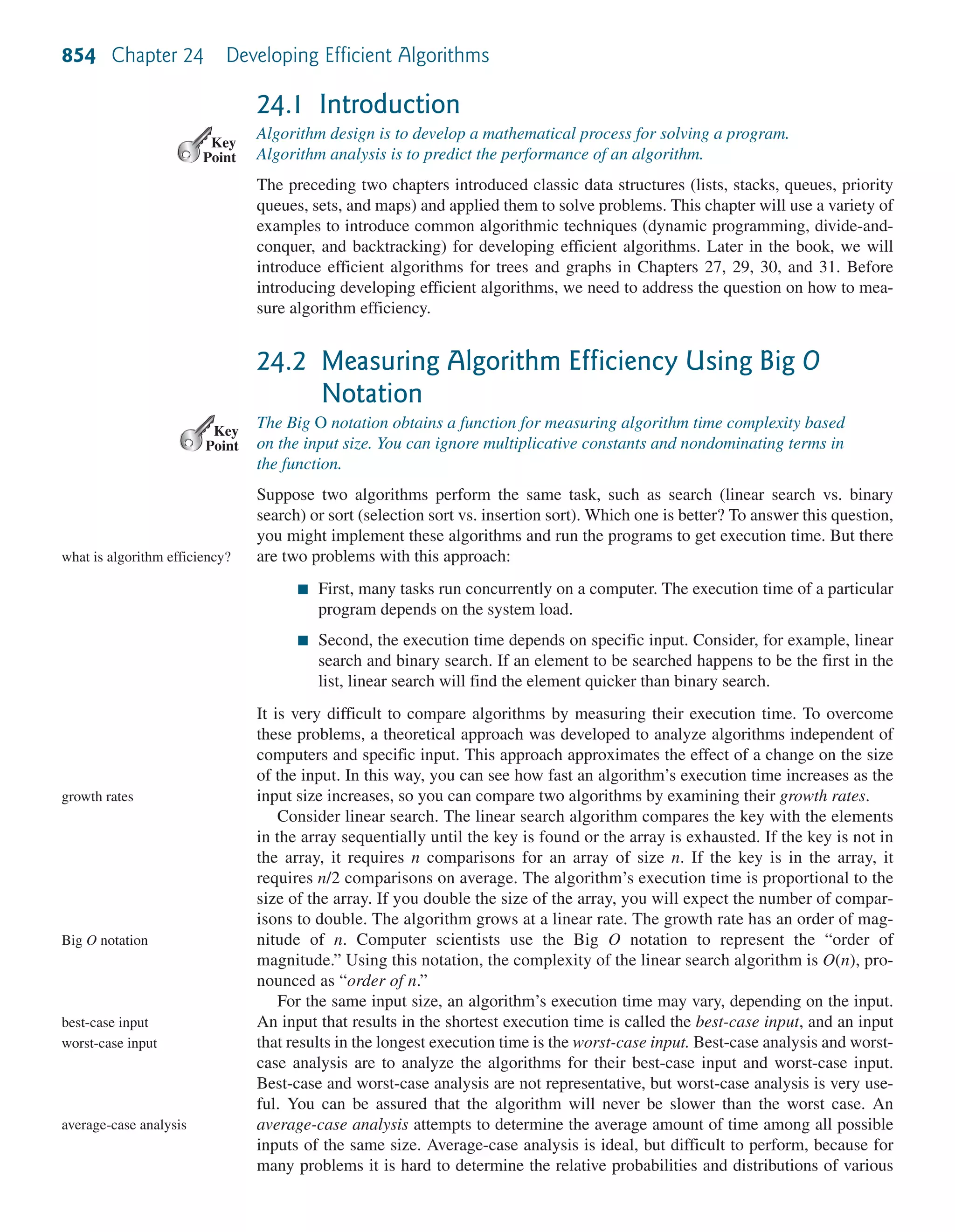
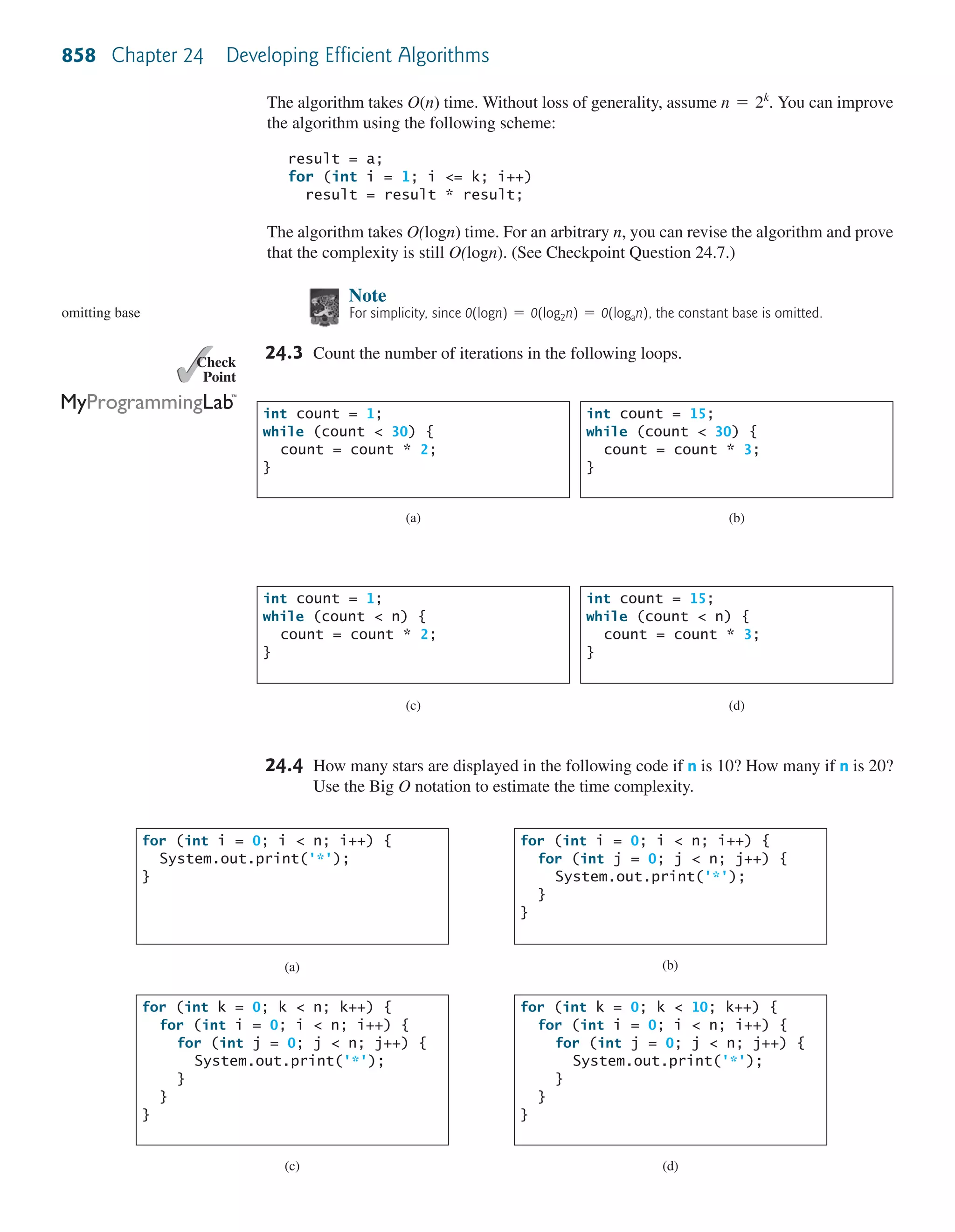
Figure 24.3 The values in primes are changed with each prime number k.
Therefore, the complexity of this algorithm is
This algorithm is another example of dynamic programming. The algorithm stores the
results of the subproblems in the array list and uses them later to check whether a new num-
ber is prime.
Is there any algorithm better than Let us examine the well-known Eratosthenes
algorithm for finding prime numbers. Eratosthenes (276–194 B.C.) was a Greek mathematician
who devised a clever algorithm, known as the Sieve of Eratosthenes, for finding all prime num-
bers His algorithm is to use an array named primes of n Boolean values. Initially, all ele-
ments in primes are set true. Since the multiples of 2 are not prime, set primes[2 * i] to
false for all as shown in Figure 24.3. Since we don’t care about primes[0]
and primes[1], these values are marked in the figure.*
2 … i … n/2,
… n.
O¢
n2n
logn
≤?
O¢
n2n
logn
≤.
dynamic programming
Sieve of Eratosthenes
Since the multiples of 3 are not prime, set primes[3 * i] to false for all
Because the multiples of 5 are not prime, set primes[5 * i] to false for all
Note that you don’t need to consider the multiples of 4, because the multiples of 4 are also the
multiples of 2, which have already been considered. Similarly, multiples of 6, 8, and 9 need
not be considered. You only need to consider the multiples of a prime number k = 2, 3, 5, 7,
11, . . . , and set the corresponding element in primes to false. Afterward, if primes[i]
is still true, then i is a prime number. As shown in Figure 24.3, 2, 3, 5, 7, 11, 13, 17, 19, and
23 are prime numbers. Listing 24.6 gives the program for finding the prime numbers using the
Sieve of Eratosthenes algorithm.
LISTING 24.6 SieveOfEratosthenes.java
2
3 public class SieveOfEratosthenes {
8
9 // Prime number sieve
10
11 // Initialize primes[i] to true
12 for (int i = 0; i < primes.length; i++) {
13
14 }
15
16 for (int k = 2; k <= n / k; k++) {
17 if (primes[k]) {
18 for (int i = k; i <= n / k; i++) {
19 // k * i is not primeprimes[k * i] = false;
primes[i] = true;
boolean[] primes = new boolean[n + 1];
5 … i … n/5.
3 … i … n/3.
sieve
initialize sieve
nonprime

20 }
21 }
22 }
23
24 int count = 0; // Count the number of prime numbers found so far
25 // Print prime numbers
26 for (int i = 2; i < primes.length; i++) {
27 if (primes[i]) {
28 count++;
29 if (count % 10 == 0)
30 System.out.printf("%7dn", i);
31 else
32 System.out.printf("%7d", i);
33 }
34 }
35
38 }
39 }
2 3 5 7 11 13 17 19 23 29
31 37 41 43 47 53 59 61 67 71
...
...
1000
Note that k <= n / k (line 16). Otherwise, k * i would be greater than n (line 19). What
is the time complexity of this algorithm?
For each prime number k (line 17), the algorithm sets primes[k * i] to false (line 19).
This is performed n / k – k + 1 times in the for loop (line 18). Thus, the complexity for
finding all prime numbers up to n is
This upper bound is very loose. The actual time complexity is much better than
The Sieve of Eratosthenes algorithm is good for a small n such that the array
primes can fit in the memory.
Table 24.5 summarizes the complexity of these three algorithms for finding all prime num-
bers up to n.
O¢
n2n
logn
≤.
O¢
n2n
logn
≤
= O¢n
2n
logn
≤
= O¢
n
2
+
n
3
+
n
5
+
n
7
+
n
11
+ . . .≤ 6 O(np(n))
n
2
- 2 + 1 +
n
3
- 3 + 1 +
n
5
- 5 + 1 +
n
7
- 7 + 1 +
n
11
- 11 + 1. . .

24.8 Finding the Closest Pair of Points Using Divide-and-Conquer 875
TABLE 24.5 Comparisons of Prime-Number Algorithms
Algorithm Complexity Description
Listing 4.14 O(n2
) Brute-force, checking all possible divisors
Listing 24.4 O(n2n) Checking divisors up to 2n
Listing 24.5 O¢
n2n
logn
≤ Checking prime divisors up to 2n
Listing 24.6 O¢
n2n
logn
≤ Sieve of Eratosthenes
✓Point✓Check
Key
Point
FIGURE 24.4 The closet-pair animation draws a line to connect the closest pair of points
dynamically as points are added and removed interactively.
24.16 Prove that if n is not prime, there must exist a prime number p such that
and p is a factor of n.
24.17 Describe how the sieve of Eratosthenes is used to find the prime numbers.
24.8 Finding the Closest Pair of Points Using Divide-
and-Conquer
This section presents efficient algorithms for finding the closest pair of points using
divide-and-conquer.
Given a set of points, the closest-pair problem is to find the two points that are nearest to each
other. As shown in Figure 24.4, a line is drawn to connect the two nearest points in the closest-
pair animation.
p 6= 2n
Section 7.6, Case Study: Finding the Closest Pair, presented a brute-force algorithm for
finding the closest pair of points. The algorithm computes the distances between all pairs of
points and finds the one with the minimum distance. Clearly, the algorithm takes time.
Can we design a more efficient algorithm?
We will use an approach called divide-and-conquer to solve this problem. The approach
divides the problem into subproblems, solves the subproblems, then combines the solutions
of the subproblems to obtain the solution for the entire problem. Unlike the dynamic pro-
gramming approach, the subproblems in the divide-and-conquer approach don’t overlap. A
subproblem is like the original problem with a smaller size, so you can apply recursion to
solve the problem. In fact, all the solutions for recursive problems follow the divide-and-
conquer approach.
Listing 24.7 describes how to solve the closest pair problem using the divide-and-
conquer approach.
O(n2
)
closest-pair animation on
Companion Website
divide-and-conquer

mid
d2
d1
d
(a) (b) (c)
d
stripL stripR
S1 S2
d d
stripL stripR
p d p
q[r]
stripL stripR
FIGURE 24.5 The midpoint divides the points into two sets of equal size.
LISTING 24.7 Algorithm for Finding the Closest Pair
Step 1: Sort the points in increasing order of x-coordinates. For the
points with the same x-coordinates, sort on y-coordinates. This results
in a sorted list S of points.
Step 2: Divide S into two subsets, S1 and S2, of equal size using the
midpoint in the sorted list. Let the midpoint be in S1. Recursively find
the closest pair in S1 and S2. Let d1 and d2 denote the distance of the
closest pairs in the two subsets, respectively.
Step 3: Find the closest pair between a point in S1 and a point in S2 and
denote their distance as d3. The closest pair is the one with the dis-
tance min(d1, d2, d3).
Selection sort and insertion sort take time. In Chapter 25 we will introduce merge sort and
heap sort. These sorting algorithms take O(n logn) time. Step 1 can be done in O(n logn) time.
Step 3 can be done in O(n) time. Let We already know that the closest-pair
distance cannot be larger than d. For a point in and a point in to form the closest pair in S,
the left point must be in stripL and the right point in stripR, as illustrated in Figure 24.5a.
For a point p in stripL, you need only consider a right point within the rectangle,
as shown in 24.5b. Any right point outside the rectangle cannot form the closest pair with p.
Since the closest-pair distance in is greater than or equal to d, there can be at most six
points in the rectangle. Thus, for each point in stripL, at most six points in stripR need to
be considered.
S2
d * 2d
S2S1
d = min(d1, d2).
O(n2
)
For each point p in stripL, how do you locate the points in the corresponding rec-
tangle area in stripR? This can be done efficiently if the points in stripL and stripR are
sorted in increasing order of their y-coordinates. Let pointsOrderedOnY be the list of the
points sorted in increasing order of y-coordinates. pointsOrderedOnY can be obtained
beforehand in the algorithm. stripL and stripR can be obtained from
pointsOrderedOnY in Step 3 as shown in Listing 24.8.
LISTING 24.8 Algorithm for Obtaining stripL
and stripR
1 for each point p in pointsOrderedOnY
2 if (p is in S1 and mid.x – p.x <= d)
3 append p to stripL;
4 else if (p is in S2 and p.x - mid.x <= d)
5 append p to stripR;
d * 2d
stripL
stripR

24.9 Solving the Eight Queen Problem Using Backtracking 877
✓Point✓Check
Key
Point
Let the points in stripL and stripR be and as shown in
Figure 24.5c. The closest pair between a point in stripL and a point in stripR can be found
using the algorithm described in Listing 24.9.
LISTING 24.9 Algorithm for Finding the Closest Pair
in Step 3
1 d = min(d1, d2);
2 r = 0; // r is the index in stripR
3 for (each point p in stripL) {
4 // Skip the points below the rectangle area
5 while (r < stripR.length && q[r].y <= p.y - d)
6 r++;
7
8 let r1 = r;
9 while (r1 < stripR.length && |q[r1].y – p.y| <= d) {
10 // Check if (p, q[r1]) is a possible closest pair
11 if (distance(p, q[r1]) < d) {
12 d = distance(p, q[r1]);
13 (p, q[r1]) is now the current closest pair;
14 }
15
16 r1 = r1 + 1;
17 }
18 }
The points in stripL are considered from in this order. For a point p in
stripL, skip the points in stripR that are below p.y – d (lines 5–6). Once a point is
skipped, it will no longer be considered. The while loop (lines 9–17) checks whether (p,
q[r1]) is a possible closest pair. There are at most six such q[r1] pairs, so the complexity
for finding the closest pair in Step 3 is O(n).
Let T(n) denote the time complexity for this algorithm. Thus,
Therefore, the closest pair of points can be found in O(n logn) time. The complete implemen-
tation of this algorithm is left as an exercise (see Programming Exercise 24.7).
24.18 What is the divide-and-conquer approach? Give an example.
24.19 What is the difference between divide-and-conquer and dynamic programming?
24.20 Can you design an algorithm for finding the minimum element in a list using divide-
and-conquer? What is the complexity of this algorithm?
24.9 Solving the Eight Queens Problem Using
Backtracking
This section solves the Eight Queens problem using the backtracking approach.
The Eight Queens problem, introduced in Programming Exercise 20.34, is to find a solution
to place a queen in each row on a chessboard such that no two queens can attack each other.
The problem was solved using recursion. In this section, we will introduce a common algo-
rithm design technique called backtracking for solving this problem. The backtracking
approach searches for a candidate solution incrementally, abandoning that option as soon as
it determines that the candidate cannot possibly be a valid solution, and then looks for a
new candidate.
T(n) = 2T(n/2) + O(n) = O(n logn)
p0, p1, . . . , pk
{q0, q1, c , qt},{p0, p1, c , pk}
update closest pair
backtracking

(a) (b)
0
4
7
5
2
6
1
3
queens[0]
queens[1]
queens[2]
queens[3]
queens[4]
queens[5]
queens[6]
queens[7]
Figure 24.6 queens[i] denotes the position of the queen in row i.
You can use a two-dimensional array to represent a chessboard. However, since each row
can have only one queen, it is sufficient to use a one-dimensional array to denote the position
of the queen in the row. Thus, you can define the queens array as:
int[] queens = new int[8];
Assign j to queens[i] to denote that a queen is placed in row i and column j. Figure 24.6a
shows the contents of the queens array for the chessboard in Figure 24.6b.
The search starts from the first row with where k is the index of the current row
being considered. The algorithm checks whether a queen can be possibly placed in the jth col-
umn in the row for in this order. The search is implemented as follows:
■ If successful, it continues to search for a placement for a queen in the next row. If the
current row is the last row, a solution is found.
■ If not successful, it backtracks to the previous row and continues to search for a new
placement in the next column in the previous row.
■ If the algorithm backtracks to the first row and cannot find a new placement for a
queen in this row, no solution can be found.
To see how the algorithm works, go to www.cs.armstrong.edu/liang/animation/
EightQueensAnimation.html.
Listing 24.10 gives the program that displays a solution for the Eight Queens problem.
LISTING 24.10 EightQueens.java
1 import java.awt.*;
2 import javax.swing.*;
3
4 public class EightQueens extends JApplet {
5 public static final int SIZE = 8; // The size of the chessboard
6 // queens are placed at (i, queens[i])
7 // -1 indicates that no queen is currently placed in the ith row
8 // Initially, place a queen at (0, 0) in the 0th row
9 private int[] queens = {-1, -1, -1, -1, -1, -1, -1, -1};
10
11 public EightQueens() {
12 if (search()) // Search for a solution
13 add(new ChessBoard(), BorderLayout.CENTER);
14 else
15 JOptionPane.showMessageDialog(null, "No solution found");
16 }
17
18 /** Search for a solution */
j = 0, 1, c , 7,
k = 0,search algorithm
Eight Queens animation on
initialize the board
search for solution

24.9 Solving the Eight Queen Problem Using Backtracking 879
19 private boolean search() {
20 // k - 1 indicates the number of queens placed so far
21 // We are looking for a position in the kth row to place a queen
22 int k = 0;
23 while (k >= 0 && k <= 7) {
24 // Find a position to place a queen in the kth row
25 int j = findPosition(k);
26 if (j < 0) {
27 queens[k] = -1;
28 k--; // back track to the previous row
29 } else {
30 queens[k] = j;
31 k++;
32 }
33 }
34
35 if (k == -1)
36 return false; // No solution
37 else
38 return true; // A solution is found
39 }
40
41 public int findPosition(int k) {
42 int start = queens[k] + 1; // Search for a new placement
43
44 for (int j = start; j < 8; j++) {
45 if (isValid(k, j))
46 return j; // (k, j) is the place to put the queen now
47 }
48
49 return -1;
50 }
51
52 /** Return true if a queen can be placed at (row, column) */
53 public boolean isValid(int row, int column) {
54 for (int i = 1; i <= row; i++)
55 if (queens[row - i] == column // Check column
56 || queens[row - i] == column - i // Check up-left diagonal
57 || queens[row - i] == column + i) // Check up-right diagonal
58 return false; // There is a conflict
59 return true; // No conflict
60 }
61
62 class ChessBoard extends JPanel {
63 private java.net.URL url
64 = getClass().getResource("image/queen.jpg");
65 private Image queenImage = new ImageIcon(url).getImage();
66
67 ChessBoard() {
68 setBorder(BorderFactory.createLineBorder(Color.BLACK, 2));
69 }
70
71 @Override
72 protected void paintComponent(Graphics g) {
73 super.paintComponent(g);
74
75 // Paint the queens
76 for (int i = 0; i < SIZE; i++) {
77 int j = queens[i]; // The position of the queen in row i
78 g.drawImage(queenImage, j * getWidth() / SIZE,
find a column
backtrack
place a queen
search the next row

0 1 2 3 4 5 6 7
0
1
2
3
4
5
6
7
upright diagonal
check
column
upleft
(row, column)
Figure 24.7 Invoking isValid(row, column) checks whether a queen can be placed at
(row, column).
✓Point✓Check
Key
Point
79 i * getHeight() / SIZE, getWidth() / SIZE,
80 getHeight() / SIZE, this);
81 }
82
83 // Draw the horizontal and vertical lines
84 for (int i = 1; i < SIZE; i++) {
85 g.drawLine(0, i * getHeight() / SIZE,
86 getWidth(), i * getHeight() / SIZE);
87 g.drawLine(i * getWidth() / SIZE, 0,
88 i * getWidth() / SIZE, getHeight());
89 }
90 }
91 }
92 }
The program invokes search() (line 12) to search for a solution. Initially, no queens are
placed in any rows (line 9). The search now starts from the first row with k = 0 (line 22) and
finds a place for the queen (line 25). If successful, place it in the row (line 30) and consider the
next row (line 31). If not successful, backtrack to the previous row (lines 27–28).
The findPosition(k) method searches for a possible position to place a queen in row k
starting from queen[k] + 1 (line 42). It checks whether a queen can be placed at start,
start + 1, . . . , and 7, in this order (lines 44–47). If possible, return the column index (line
46); otherwise, return -1 (line 49).
The isValid(row, column) method is called to check whether placing a queen at the
specified position causes a conflict with the queens placed earlier (line 45). It ensures that no
queen is placed in the same column (line 55), in the upper-left diagonal (line 56), or in the
upper-right diagonal (line 57), as shown in Figure 24.7.
24.21 What is backtracking? Give an example.
24.22 If you generalize the Eight Queens problem to the n-Queens problem in an n-by-n
chessboard, what will be the complexity of the algorithm?
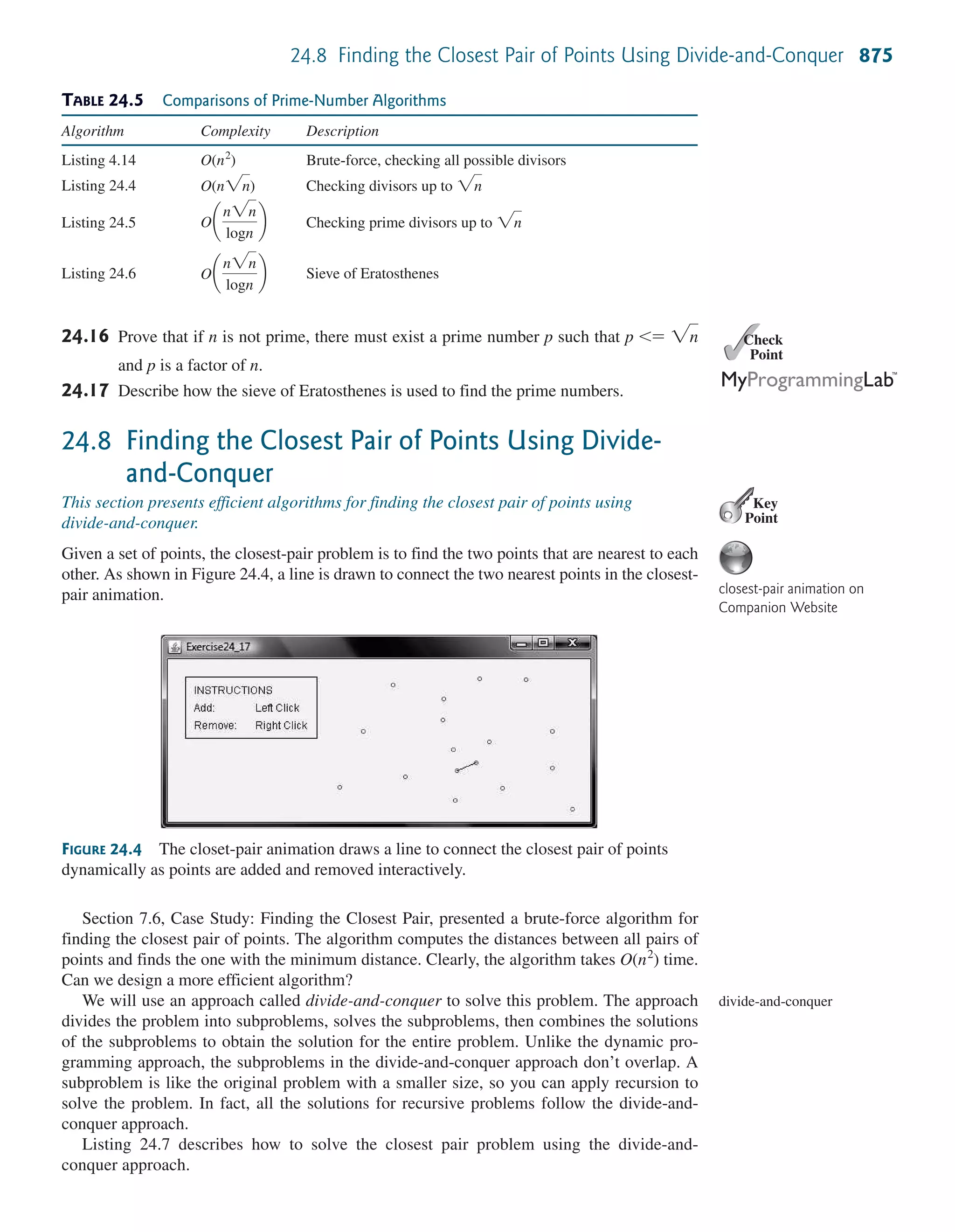
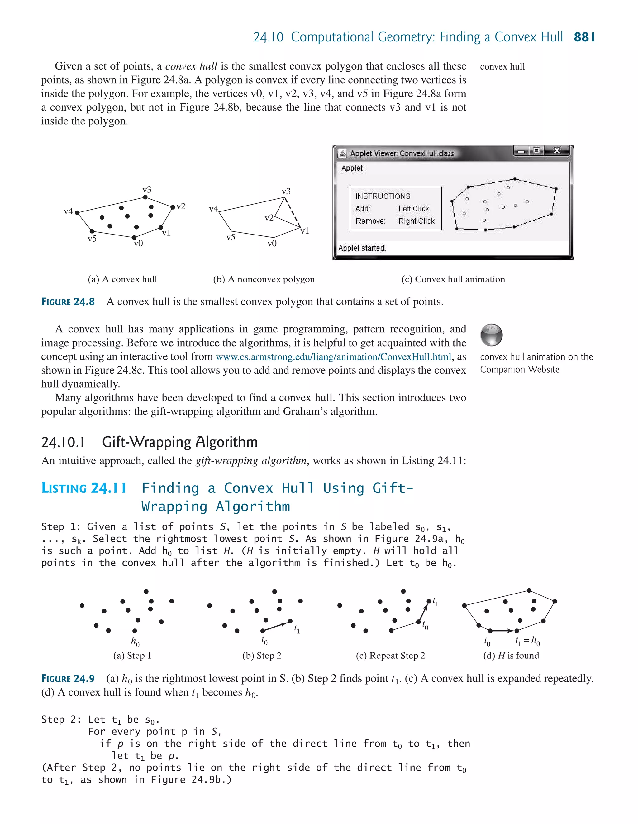
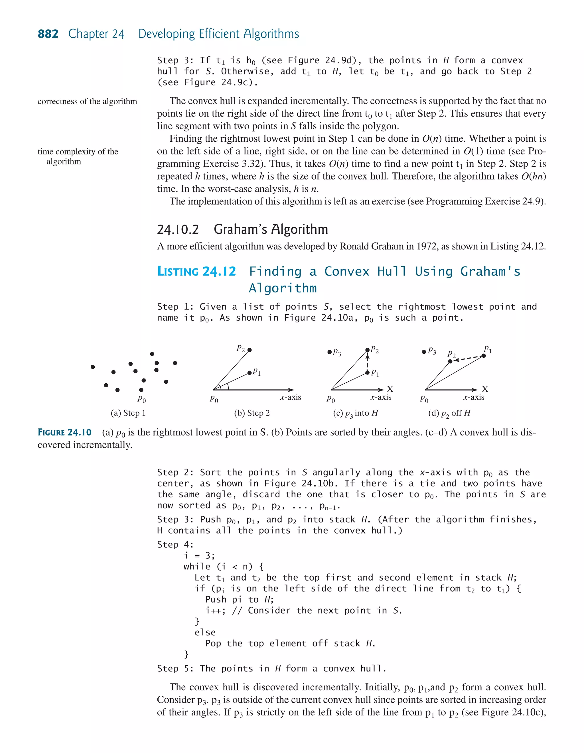
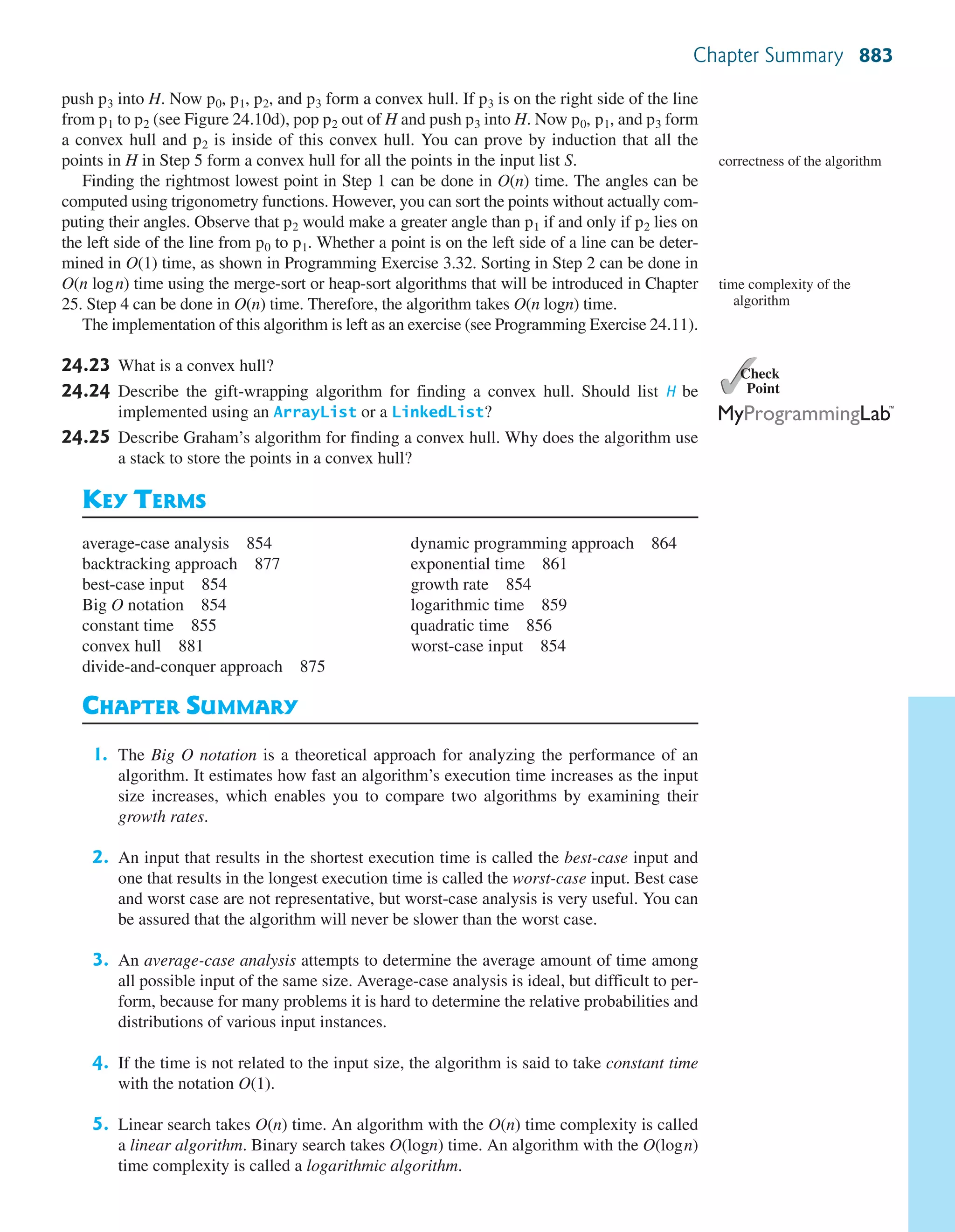
24.10 Computational Geometry: Finding a Convex Hull
This section presents efficient geometric algorithms for finding a convex hull for a
set of points.
Computational geometry is to study the algorithms for geometrical problems. It has applica-
tions in computer graphics, games, pattern recognition, image processing, robotics, geograph-
ical information systems, and computer-aided design and manufacturing. Section 24.8
presented a geometrical algorithm for finding the closest pair of points. This section intro-
duces geometrical algorithms for finding a convex hull.
main method omitted

24.10 Computational Geometry: Finding a Convex Hull 881
(a) A convex hull (b) A nonconvex polygon (c) Convex hull animation
v3
v2
v1
v4
v5
v0
v1
v3
v2
v0v5
v4
FIGURE 24.8 A convex hull is the smallest convex polygon that contains a set of points.
(a) Step 1 (b) Step 2 (c) Repeat Step 2 (d) H is found
t1
= h0t0
t0
t1
t1
t0h0
FIGURE 24.9 (a) is the rightmost lowest point in S. (b) Step 2 finds point (c) A convex hull is expanded repeatedly.
(d) A convex hull is found when becomes h0.t1
t1.h0
Given a set of points, a convex hull is the smallest convex polygon that encloses all these
points, as shown in Figure 24.8a. A polygon is convex if every line connecting two vertices is
inside the polygon. For example, the vertices v0, v1, v2, v3, v4, and v5 in Figure 24.8a form
a convex polygon, but not in Figure 24.8b, because the line that connects v3 and v1 is not
inside the polygon.
convex hull
convex hull animation on the
Companion Website
A convex hull has many applications in game programming, pattern recognition, and
image processing. Before we introduce the algorithms, it is helpful to get acquainted with the
concept using an interactive tool from www.cs.armstrong.edu/liang/animation/ConvexHull.html, as
shown in Figure 24.8c. This tool allows you to add and remove points and displays the convex
hull dynamically.
Many algorithms have been developed to find a convex hull. This section introduces two
popular algorithms: the gift-wrapping algorithm and Graham’s algorithm.
24.10.1 Gift-Wrapping Algorithm
An intuitive approach, called the gift-wrapping algorithm, works as shown in Listing 24.11:
LISTING 24.11 Finding a Convex Hull Using Gift-
Wrapping Algorithm
Step 1: Given a list of points S, let the points in S be labeled s0, s1,
..., sk. Select the rightmost lowest point S. As shown in Figure 24.9a, h0
is such a point. Add h0 to list H. (H is initially empty. H will hold all
points in the convex hull after the algorithm is finished.) Let t0 be h0.
Step 2: Let t1 be s0.
For every point p in S,
if p is on the right side of the direct line from t0 to t1, then
let t1 be p.
(After Step 2, no points lie on the right side of the direct line from t0
to t1, as shown in Figure 24.9b.)

(a) Step 1 (b) Step 2 (c) p3
into H (d) p2
off H
p0
p0
p0
p0
XX
p1 p1
p1
p2 p2 p2
p3
p3
x-axis x-axis x-axis
FIGURE 24.10 (a) is the rightmost lowest point in S. (b) Points are sorted by their angles. (c–d) A convex hull is dis-
covered incrementally.
p0
Step 3: If t1 is h0 (see Figure 24.9d), the points in H form a convex
hull for S. Otherwise, add t1 to H, let t0 be t1, and go back to Step 2
(see Figure 24.9c).
The convex hull is expanded incrementally. The correctness is supported by the fact that no
points lie on the right side of the direct line from to after Step 2. This ensures that every
line segment with two points in S falls inside the polygon.
Finding the rightmost lowest point in Step 1 can be done in O(n) time. Whether a point is
on the left side of a line, right side, or on the line can be determined in O(1) time (see Pro-
gramming Exercise 3.32). Thus, it takes O(n) time to find a new point in Step 2. Step 2 is
repeated h times, where h is the size of the convex hull. Therefore, the algorithm takes O(hn)
time. In the worst-case analysis, h is n.
The implementation of this algorithm is left as an exercise (see Programming Exercise 24.9).
24.10.2 Graham’s Algorithm
A more efficient algorithm was developed by Ronald Graham in 1972, as shown in Listing 24.12.
LISTING 24.12 Finding a Convex Hull Using Graham's
Algorithm
Step 1: Given a list of points S, select the rightmost lowest point and
name it p0. As shown in Figure 24.10a, p0 is such a point.
t1
t1t0
correctness of the algorithm
time complexity of the
algorithm
Step 2: Sort the points in S angularly along the x-axis with p0 as the
center, as shown in Figure 24.10b. If there is a tie and two points have
the same angle, discard the one that is closer to p0. The points in S are
now sorted as p0, p1, p2, ..., pn-1.
Step 3: Push p0, p1, and p2 into stack H. (After the algorithm finishes,
H contains all the points in the convex hull.)
Step 4:
i = 3;
while (i < n) {
Let t1 and t2 be the top first and second element in stack H;
if (pi is on the left side of the direct line from t2 to t1) {
Push pi to H;
i++; // Consider the next point in S.
}
else
Pop the top element off stack H.
}
Step 5: The points in H form a convex hull.
The convex hull is discovered incrementally. Initially, and form a convex hull.
Consider is outside of the current convex hull since points are sorted in increasing order
of their angles. If is strictly on the left side of the line from to (see Figure 24.10c),p2p1p3
p3. p3
p2p0, p1,

Chapter Summary 883
✓Point✓Check
push into H. Now and form a convex hull. If is on the right side of the line
from to (see Figure 24.10d), pop out of H and push into H. Now and form
a convex hull and is inside of this convex hull. You can prove by induction that all the
points in H in Step 5 form a convex hull for all the points in the input list S.
Finding the rightmost lowest point in Step 1 can be done in O(n) time. The angles can be
computed using trigonometry functions. However, you can sort the points without actually com-
puting their angles. Observe that would make a greater angle than if and only if lies on
the left side of the line from to Whether a point is on the left side of a line can be deter-
mined in O(1) time, as shown in Programming Exercise 3.32. Sorting in Step 2 can be done in
O(n logn) time using the merge-sort or heap-sort algorithms that will be introduced in Chapter
25. Step 4 can be done in O(n) time. Therefore, the algorithm takes O(n logn) time.
The implementation of this algorithm is left as an exercise (see Programming Exercise 24.11).
24.23 What is a convex hull?
24.24 Describe the gift-wrapping algorithm for finding a convex hull. Should list H be
implemented using an ArrayList or a LinkedList?
24.25 Describe Graham’s algorithm for finding a convex hull. Why does the algorithm use
a stack to store the points in a convex hull?
KEY TERMS
p1.p0
p2p1p2
p2
p3p0, p1,p3p2p2p1
p3p3p0, p1, p2,p3
correctness of the algorithm
time complexity of the
algorithm
average-case analysis 854
backtracking approach 877
best-case input 854
Big O notation 854
constant time 855
convex hull 881
divide-and-conquer approach 875
dynamic programming approach 864
exponential time 861
growth rate 854
logarithmic time 859
quadratic time 856
worst-case input 854
CHAPTER SUMMARY
1. The Big O notation is a theoretical approach for analyzing the performance of an
algorithm. It estimates how fast an algorithm’s execution time increases as the input
size increases, which enables you to compare two algorithms by examining their
growth rates.
2. An input that results in the shortest execution time is called the best-case input and
one that results in the longest execution time is called the worst-case input. Best case
and worst case are not representative, but worst-case analysis is very useful. You can
be assured that the algorithm will never be slower than the worst case.
3. An average-case analysis attempts to determine the average amount of time among
all possible input of the same size. Average-case analysis is ideal, but difficult to per-
form, because for many problems it is hard to determine the relative probabilities and
distributions of various input instances.
4. If the time is not related to the input size, the algorithm is said to take constant time
with the notation O(1).
5. Linear search takes O(n) time. An algorithm with the O(n) time complexity is called
a linear algorithm. Binary search takes O(logn) time. An algorithm with the O(logn)
time complexity is called a logarithmic algorithm.

6. The worst-time complexity for selection sort and insertion sort is An algorithm
with the time complexity is called a quadratic algorithm.
7. The time complexity for the Towers of Hanoi problem is An algorithm with
the time complexity is called an exponential algorithm.
8. A Fibonacci number at a given index can be found in O(n) time using dynamic
programming.
9. Dynamic programming is the process of solving subproblems, then combining the
solutions of the subproblems to obtain an overall solution. The key idea behind
dynamic programming is to solve each subproblem only once and store the results for
subproblems for later use to avoid redundant computing of the subproblems.
10. Euclid’s GCD algorithm takes O(logn) time.
11. All prime numbers less than or equal to n can be found in time.
12. The closest pair can be found in O(n logn) time using the divide-and-conquer approach.
13. The divide-and-conquer approach divides the problem into subproblems, solves
the subproblems, then combines the solutions of the subproblems to obtain the
solution for the entire problem. Unlike the dynamic programming approach, the
subproblems in the divide-and-conquer approach don’t overlap. A subproblem is
like the original problem with a smaller size, so you can apply recursion to solve
the problem.
14. The Eight Queens problem can be solved using backtracking.
15. The backtracking approach searches for a candidate solution incrementally, abandon-
ing that option as soon as it determines that the candidate cannot possibly be a valid
solution, and then looks for a new candidate.
16. A convex hull for a set of points can be found in time using the gift-wrapping
algorithm and in O(n logn) time using the Graham’s algorithm.
TEST QUESTIONS
Do the test questions for this chapter online at www.cs.armstrong.edu/liang/intro9e/test.html.
PROGRAMMING EXERCISES
*24.1 (Maximum consecutive increasingly ordered substring) Write a program that
prompts the user to enter a string and displays the maximum consecutive increas-
ingly ordered substring. Analyze the time complexity of your program. Here is a
sample run:
O(n2
)
O¢
n2n
logn
≤
O(2n
)
O(2n
).
O(n2
)
O(n2
).
Enter a string:
Wel
Welcome

40 41 42 43 44 45
Listing 24.2 GCD
Listing 24.3 GCDEuclid
Programming Exercises 885
**24.2 (Maximum increasingly ordered subsequence) Write a program that prompts the
user to enter a string and displays the maximum increasingly ordered subsequence
of characters. Analyze the time complexity of your program. Here is a sample run:
Enter a string:
Welo
Welcome
*24.3 (Pattern matching) Write a program that prompts the user to enter two strings and
tests whether the second string is a substring of the first string. Suppose the neigh-
boring characters in the string are distinct. (Don’t use the indexOf method in the
String class.) Analyze the time complexity of your algorithm. Your algorithm
needs to be at least O(n) time. Here is a sample run of the program:
Enter a string s1:
Enter a string s2:
matched at index 3
come
Welcome to Java
*24.4 (Pattern matching) Write a program that prompts the user to enter two strings and
tests whether the second string is a substring of the first string. (Don’t use the
indexOf method in the String class.) Analyze the time complexity of your algo-
rithm. Here is a sample run of the program:
Enter a string s1:
Enter a string s2:
matched at index 6
sip
Mississippi
*24.5 (Same-number subsequence) Write an O(n) program that prompts the user to enter
a sequence of integers ending with 0 and finds the longest subsequence with the
same number. Here is a sample run of the program:
Enter a series of numbers ending with 0:
The longest same number sequence starts at index 3 with 4
values of 8
2 4 4 8 8 8 8 2 4 4 0
*24.6 (Execution time for GCD) Write a program that obtains the execution time for
finding the GCD of every two consecutive Fibonacci numbers from the index 40 to
index 45 using the algorithms in Listings 24.2 and 24.3. Your program should
print a table like this:
(Hint: You can use the following code template to obtain the execution time.)
long startTime = System.currentTimeMillis();
perform the task;
long endTime = System.currentTimeMillis();
long executionTime = endTime - startTime;

**24.7 (Closest pair of points) Section 24.8 introduced an algorithm for finding the clos-
est pair of points using a divide-and-conquer approach. Implement the algorithm
to meet the following requirements:
■ Define the classes Point and CompareY in the same way as in Programming
Exercise 22.4.
■ Define a class named Pair with the data fields p1 and p2 to represent two
points, and a method named getDistance() that returns the distance between
the two points.
■ Implement the following methods:
/** Return the distance of the closest pair of points */
public static Pair getClosestPair(double[][] points)
/** Return the distance of the closest pair of points */
public static Pair getClosestPair(Point[] points)
/** Return the distance of the closest pair of points
* in pointsOrderedOnX[low..high]. This is a recursive
* method. pointsOrderedOnX and pointsOrderedOnY are
* not changed in the subsequent recursive calls.
*/
public static Pair distance(Point[] pointsOrderedOnX,
int low, int high, Point[] pointsOrderedOnY)
/** Compute the distance between two points p1 and p2 */
public static double distance(Point p1, Point p2)
/** Compute the distance between points (x1, y1) and (x2, y2) */
public static double distance(double x1, double y1,
double x2, double y2)
**24.8 (All prime numbers up to 10,000,000,000) Write a program that finds all prime
numbers up to 10,000,000,000. There are approximately 455,052,511 such
prime numbers. Your program should meet the following requirements:
■ Your program should store the prime numbers in a binary data file, named
PrimeNumbers.dat. When a new prime number is found, the number is
appended to the file.
■ To find whether a new number is prime, your program should load the prime
numbers from the file to an array of the long type of size 10000. If no number
in the array is a divisor for the new number, continue to read the next 10000
prime numbers from the data file, until a divisor is found or all numbers in the
file are read. If no divisor is found, the new number is prime.
■ Since this program takes a long time to finish, you should run it as a batch job
from a UNIX machine. If the machine is shut down and rebooted, your program
should resume by using the prime numbers stored in the binary data file rather
than start over from scratch.
**24.9 (Geometry: gift-wrapping algorithm for finding a convex hull) Section 24.10.1
introduced the gift-wrapping algorithm for finding a convex hull for a set of
points. Assume that the Java’s coordinate system is used for the points. Implement
the algorithm using the following method:
/** Return the points that form a convex hull */
public static ArrayList<MyPoint> getConvexHull(double[][] s)

MyPoint is a static inner class defined as follows:
static class MyPoint {
double x, y;
MyPoint(double x, double y) {
this.x = x; this.y = y;
}
}
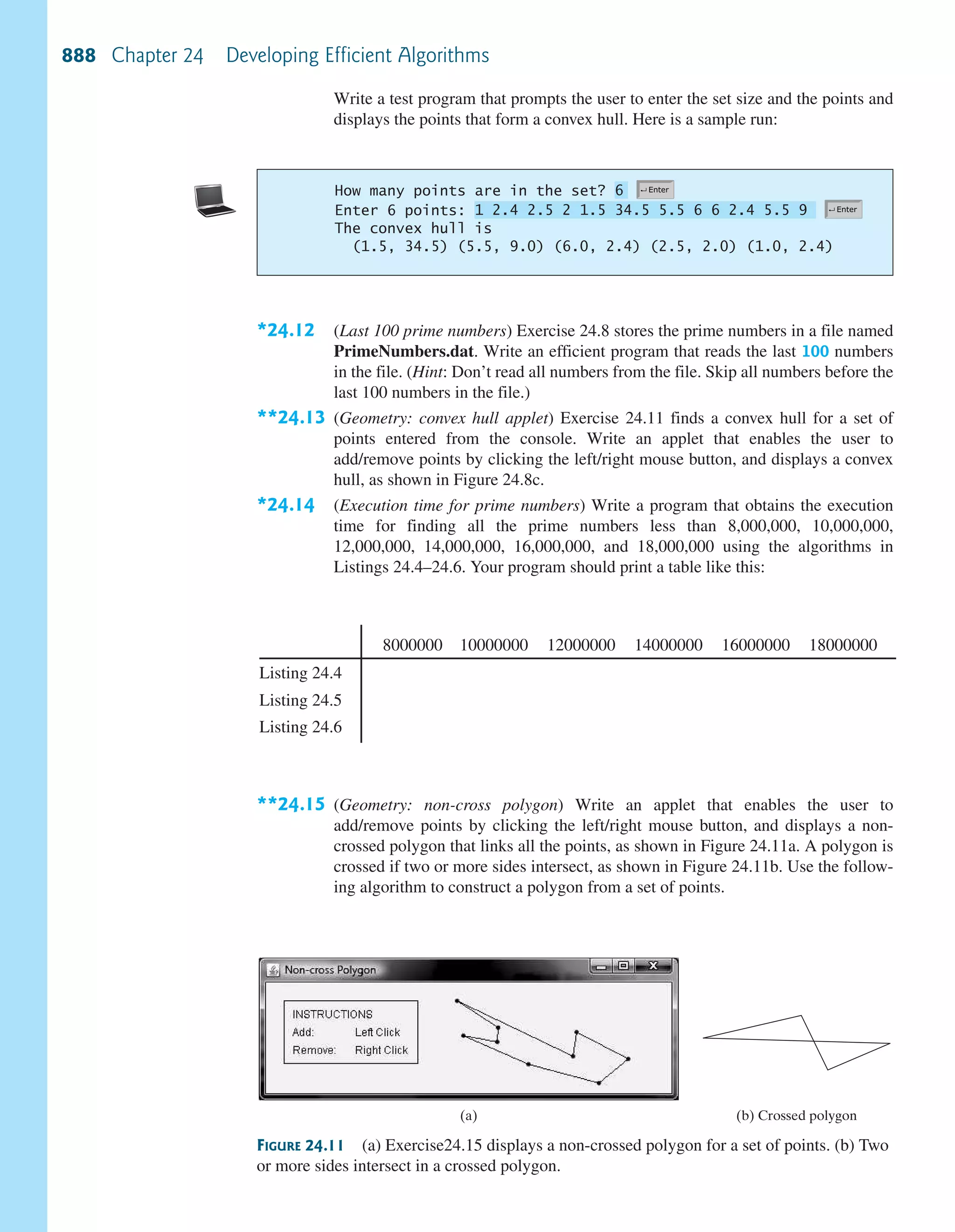
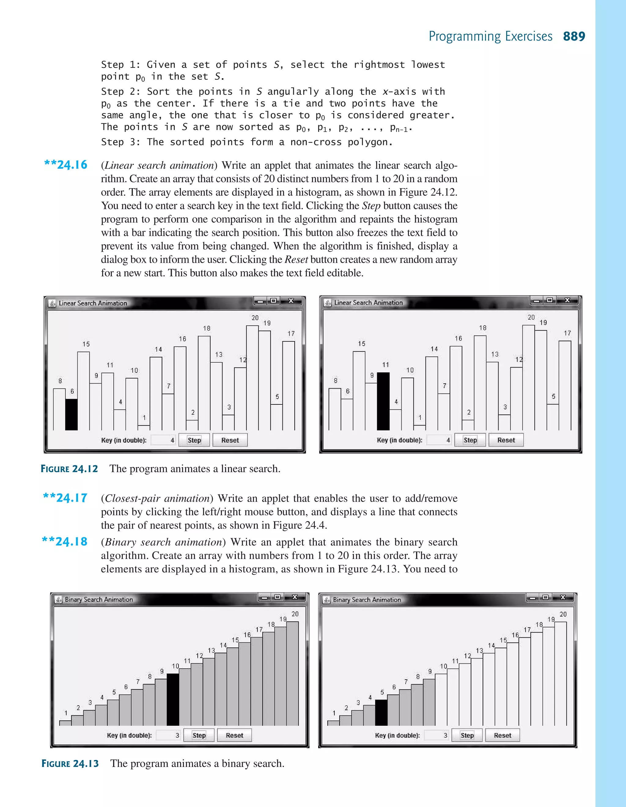
Write a test program that prompts the user to enter the set size and the points and
displays the points that form a convex hull. Here is a sample run:
How many points are in the set?
Enter 6 points:
The convex hull is
(1.5, 34.5) (5.5, 9.0) (6.0, 2.4) (2.5, 2.0) (1.0, 2.4)
1 2.4 2.5 2 1.5 34.5 5.5 6 6 2.4 5.5 9
6
24.10 (Number of prime numbers) Exercise 24.8 stores the prime numbers in a file named
PrimeNumbers.dat. Write a program that finds the number of prime numbers that
are less than or equal to 10, 100, 1,000, 10,000, 100,000, 1,000,000,
10,000,000, 100,000,000, 1,000,000,000, and 10,000,000,000. Your
program should read the data from PrimeNumbers.dat. Note that the data file may
continue to grow as more prime numbers are stored in the file.
**24.11 (Geometry: Graham’s algorithm for finding a convex hull) Section 24.10.2 intro-
duced Graham’s algorithm for finding a convex hull for a set of points. Assume
that the Java’s coordinate system is used for the points. Implement the algorithm
using the following method:
/** Return the points that form a convex hull */
public static ArrayList<MyPoint> getConvexHull(double[][] s)
MyPoint is a static inner class defined as follows:
private static class MyPoint implements Comparable<MyPoint> {
double x, y;
MyPoint rightMostLowestPoint;
MyPoint(double x, double y) {
this.x = x; this.y = y;
}
public void setRightMostLowestPoint(MyPoint p) {
rightMostLowestPoint = p;
}
@Override
public int compareTo(MyPoint o) {
// Implement it to compare this point with point o
// angularly along the x-axis with rightMostLowestPoint
// as the center, as shown in Figure 24.10b. By implementing
// the Comparable interface, you can use the Array.sort
// method to sort the points to simplify coding.
}

8000000 10000000 12000000 14000000 16000000 18000000
Listing 24.4
Listing 24.5
Listing 24.6
(a) (b) Crossed polygon
FIGURE 24.11 (a) Exercise24.15 displays a non-crossed polygon for a set of points. (b) Two
or more sides intersect in a crossed polygon.
Write a test program that prompts the user to enter the set size and the points and
displays the points that form a convex hull. Here is a sample run:
How many points are in the set?
Enter 6 points:
The convex hull is
(1.5, 34.5) (5.5, 9.0) (6.0, 2.4) (2.5, 2.0) (1.0, 2.4)
1 2.4 2.5 2 1.5 34.5 5.5 6 6 2.4 5.5 9
6
*24.12 (Last 100 prime numbers) Exercise 24.8 stores the prime numbers in a file named
PrimeNumbers.dat. Write an efficient program that reads the last 100 numbers
in the file. (Hint: Don’t read all numbers from the file. Skip all numbers before the
last 100 numbers in the file.)
**24.13 (Geometry: convex hull applet) Exercise 24.11 finds a convex hull for a set of
points entered from the console. Write an applet that enables the user to
add/remove points by clicking the left/right mouse button, and displays a convex
hull, as shown in Figure 24.8c.
*24.14 (Execution time for prime numbers) Write a program that obtains the execution
time for finding all the prime numbers less than 8,000,000, 10,000,000,
12,000,000, 14,000,000, 16,000,000, and 18,000,000 using the algorithms in
Listings 24.4–24.6. Your program should print a table like this:
**24.15 (Geometry: non-cross polygon) Write an applet that enables the user to
add/remove points by clicking the left/right mouse button, and displays a non-
crossed polygon that links all the points, as shown in Figure 24.11a. A polygon is
crossed if two or more sides intersect, as shown in Figure 24.11b. Use the follow-
ing algorithm to construct a polygon from a set of points.

FIGURE 24.12 The program animates a linear search.
Step 1: Given a set of points S, select the rightmost lowest
point p0 in the set S.
Step 2: Sort the points in S angularly along the x-axis with
p0 as the center. If there is a tie and two points have the
same angle, the one that is closer to p0 is considered greater.
The points in S are now sorted as p0, p1, p2, ..., pn-1.
Step 3: The sorted points form a non-cross polygon.
**24.16 (Linear search animation) Write an applet that animates the linear search algo-
rithm. Create an array that consists of 20 distinct numbers from 1 to 20 in a random
order. The array elements are displayed in a histogram, as shown in Figure 24.12.
You need to enter a search key in the text field. Clicking the Step button causes the
program to perform one comparison in the algorithm and repaints the histogram
with a bar indicating the search position. This button also freezes the text field to
prevent its value from being changed. When the algorithm is finished, display a
dialog box to inform the user. Clicking the Reset button creates a new random array
for a new start. This button also makes the text field editable.
**24.17 (Closest-pair animation) Write an applet that enables the user to add/remove
points by clicking the left/right mouse button, and displays a line that connects
the pair of nearest points, as shown in Figure 24.4.
**24.18 (Binary search animation) Write an applet that animates the binary search
algorithm. Create an array with numbers from 1 to 20 in this order. The array
elements are displayed in a histogram, as shown in Figure 24.13. You need to
FIGURE 24.13 The program animates a binary search.

(a) (b)
FIGURE 24.14 The program finds the largest block of 1s.
enter a search key in the text field. Clicking the Step button causes the pro-
gram to perform one comparison in the algorithm. Use a light-gray color to
paint the bars for the numbers in the current search range and use a black
color to paint the a bar indicating the middle number in the search range. The
Step button also freezes the text field to prevent its value from being changed.
When the algorithm is finished, display a dialog box to inform the user.
Clicking the Reset button enables a new search to start. This button also
makes the text field editable.
*24.19 (Largest block) The problem for finding a largest block is described in Program-
ming Exercise 7.35. Design a dynamic programming algorithm for solving this
problem in time. Write a test program that displays a 10-by-10 square
matrix, as shown in Figure 24.14. Each element in the matrix is 0 or 1, randomly
generated with a click of the Refresh button. Display each number centered in a
text field. Use a text field for each entry. Allow the user to change the entry value.
Click the Find Largest Block button to find a largest square submatrix that con-
sists of 1s. Highlight the numbers in the block, as shown in Figure 24.14b. See
www.cs.armstrong.edu/liang/animation/FindLargestBlock.html for an interactive test.
O(n2
)
***24.20 (Game: multiple Sudoku solutions) The complete solution for the Sudoku prob-
lem is given in Supplement VI.A. A Sudoku problem may have multiple solu-
tions. Modify Sudoku.java in Supplement VI.A to display the total number of
the solutions. Display two solutions if multiple solutions exist.
***24.21 (Game: Sudoku) The complete solution for the Sudoku problem is given in Sup-
plement VI.A. Write a program that lets the user enter the input from the text
fields in an applet, as shown in Figure 24.15. Clicking the Solve button displays
the result.
***24.22 (Game: recursive Sudoku) Write a recursive solution for the Sudoku problem.
***24.23 (Game: multiple Eight Queens solution) Write an applet to display all possible
solutions for the Eight Queens puzzle in a scroll pane, as shown in Figure 24.16.
For each solution, put a label to denote the solution number. (Hint: Place all
solution panels into one panel and place this one panel into a JScrollPane.)

FIGURE 24.15 The program solves the Sudoku problem.
FIGURE 24.16 All solutions are placed in a scroll pane.
The solution panel class should override the getPreferredSize() method to
ensure that a solution panel is displayed properly. See Listing 13.3, Fig-
urePanel.java, for how to override getPreferredSize().
**24.24 (Find the smallest number) Write a method that uses the divide-and-conquer
approach to find the smallest number in a list.
***24.25 (Game: Sudoku) Revise Exercise 24.21 to display all solutions for the Sudoku
game, as shown in Figure 24.17a. When you click the Solve button, the pro-
gram stores all solutions in an ArrayList. Each element in the list is a two-
dimensional 9-by-9 grid. If the program has multiple solutions, the OK button
appears as shown in Figure 24.17b. You can click the Next button to display the
next solution, as shown in Figure 24.17c. When the Clear button is clicked, the
cells are cleared and the Next button is hidden.

(a) (b) (c)
FIGURE 24.17 The program can display multiple Sudoku solutions.

ALGORITHM EFFICIENCY WITH BIG O NOTATION

Recommended

Recommended

More Related Content

What's hot

What's hot (20)

Similar to ALGORITHM EFFICIENCY WITH BIG O NOTATION

Similar to ALGORITHM EFFICIENCY WITH BIG O NOTATION (20)

ALGORITHM EFFICIENCY WITH BIG O NOTATION