![Reasonable Model for 2D Images
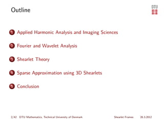
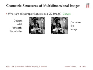
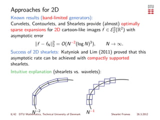
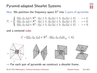
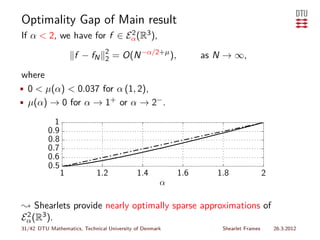
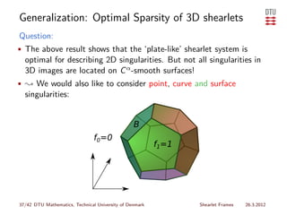
Definition (Donoho; 2001)
The set of cartoon-like 2D images E2 (R2 ) is defined by
2
E2 (R2 ) = {f ∈ L2 (R2 ) : f = f0 +f1 χB } fi ∈ C 2 (R2 ), supp fi ⊂ [0, 1]2 ,
2
where B ⊂ [0, 1]2 and the boundary curve ∂B is a closed C 2 -curve
with curvature bounded by ν.
f0=0
7/42 DTU Mathematics, Technical University of Denmark Shearlet Frames 26.3.2012](https://image.slidesharecdn.com/shearlet3dpresentation-120326034830-phpapp01/85/Shearlet-Frames-and-Optimally-Sparse-Approximations-9-320.jpg)
![Reasonable Model for 2D Images
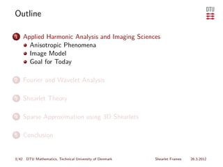
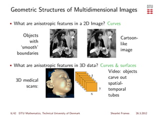
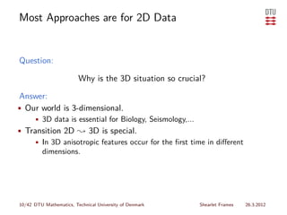
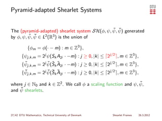
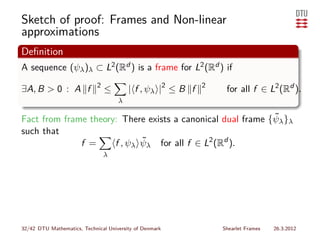
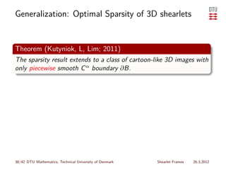
Definition (Donoho; 2001)
The set of cartoon-like 2D images E2 (R2 ) is defined by
2
E2 (R2 ) = {f ∈ L2 (R2 ) : f = f0 +f1 χB } fi ∈ C 2 (R2 ), supp fi ⊂ [0, 1]2 ,
2
where B ⊂ [0, 1]2 and the boundary curve ∂B is a closed C 2 -curve
with curvature bounded by ν.
Theorem (Donoho; 2001)
Let (ψλ )λ ⊂ L2 (R2 ). The optimal asymptotic approximation error
of f ∈ E2 (R2 ) is
2
2
f − fN 2 N −2 , N → ∞, where fN = cλ ψλ .
λ∈IN
7/42 DTU Mathematics, Technical University of Denmark Shearlet Frames 26.3.2012](https://image.slidesharecdn.com/shearlet3dpresentation-120326034830-phpapp01/85/Shearlet-Frames-and-Optimally-Sparse-Approximations-10-320.jpg)
![Reasonable Model for 3D Images
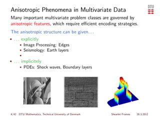
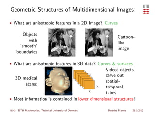
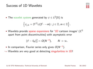
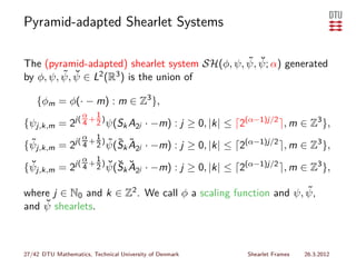
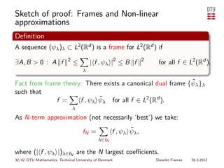
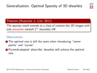
Definition
The set of 3D images E2 (R3 ) is defined by
2
E2 (R3 ) = {f ∈ L2 (R3 ) : f = f0 +f1 χB } fi ∈ C 2 (R3 ), supp fi ⊂ [0, 1]3 ,
2
where B ⊂ [0, 1]3 and the boundary surface ∂B is a closed
C 2 -surface for which the principal curvatures are bounded by ν.
f0=0
9/42 DTU Mathematics, Technical University of Denmark Shearlet Frames 26.3.2012](https://image.slidesharecdn.com/shearlet3dpresentation-120326034830-phpapp01/85/Shearlet-Frames-and-Optimally-Sparse-Approximations-13-320.jpg)
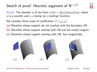
![Reasonable Model for 3D Images
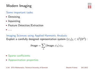
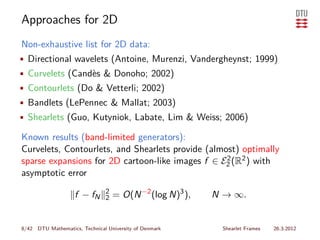
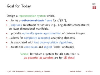
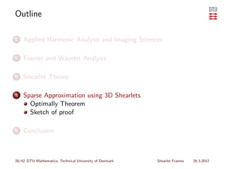
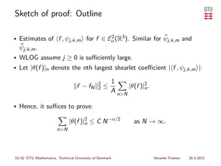
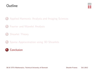
Definition
The set of 3D images E2 (R3 ) is defined by
2
E2 (R3 ) = {f ∈ L2 (R3 ) : f = f0 +f1 χB } fi ∈ C 2 (R3 ), supp fi ⊂ [0, 1]3 ,
2
where B ⊂ [0, 1]3 and the boundary surface ∂B is a closed
C 2 -surface for which the principal curvatures are bounded by ν.
Theorem (Kutyniok, L, Lim; 2011)
Let (ψλ )λ ⊂ L2 (R3 ). The optimal asymptotic approximation error
of f ∈ E2 (R3 ) is
2
2
f − fN 2 N −1 , N → ∞, where fN = cλ ψλ .
λ∈IN
9/42 DTU Mathematics, Technical University of Denmark Shearlet Frames 26.3.2012](https://image.slidesharecdn.com/shearlet3dpresentation-120326034830-phpapp01/85/Shearlet-Frames-and-Optimally-Sparse-Approximations-14-320.jpg)
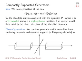
![Fourier Series
• {e2πinx }n∈Z is an ONB for L2 ([0, 1]): f = n cn e2πinx
• Modulation: En f (x) := e2πinx f (x), f ∈ L2 (R).
• Translation: Tm f (x) := f (x − m), f ∈ L2 (R).
• {En Tm χ[0,1] }n,m∈Z ONB for L2 (R): f = n,m cn,m En Tm χ[0,1]
14/42 DTU Mathematics, Technical University of Denmark Shearlet Frames 26.3.2012](https://image.slidesharecdn.com/shearlet3dpresentation-120326034830-phpapp01/85/Shearlet-Frames-and-Optimally-Sparse-Approximations-19-320.jpg)
![Fourier Series
• {e2πinx }n∈Z is an ONB for L2 ([0, 1]): f = n cn e2πinx
• Modulation: En f (x) := e2πinx f (x), f ∈ L2 (R).
• Translation: Tm f (x) := f (x − m), f ∈ L2 (R).
• {En Tm χ[0,1] }n,m∈Z ONB for L2 (R): f = n,m cn,m En Tm χ[0,1]
Simple 1D cartoon-like image (0 < x0 < x1 < 1):
1 x ∈ [x0 , x1 ] ,
f (x) =
0 otherwise
Fourier Coefficients:
1 x1 1
|cn,0 | = f (x) e−2πinx dx = e−2πinx dx ∼
0 x0 n
14/42 DTU Mathematics, Technical University of Denmark Shearlet Frames 26.3.2012](https://image.slidesharecdn.com/shearlet3dpresentation-120326034830-phpapp01/85/Shearlet-Frames-and-Optimally-Sparse-Approximations-20-320.jpg)
![1D Fourier Series Approximation
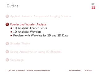
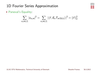
• Parseval’s Equality:
|cn,m |2 = | f , En Tm χ0,1 |2 = f 2
2
n,m∈Z n,m∈Z
• Best N-term approximation:
fN = cn,m En Tm χ[0,1] , # |IN | = N
(n,m)∈IN
15/42 DTU Mathematics, Technical University of Denmark Shearlet Frames 26.3.2012](https://image.slidesharecdn.com/shearlet3dpresentation-120326034830-phpapp01/85/Shearlet-Frames-and-Optimally-Sparse-Approximations-22-320.jpg)
![1D Fourier Series Approximation
• Parseval’s Equality:
|cn,m |2 = | f , En Tm χ0,1 |2 = f 2
2
n,m∈Z n,m∈Z
• Best N-term approximation:
fN = cn,m En Tm χ[0,1] , # |IN | = N
(n,m)∈IN
• By Parseval’s Equality:
∞ ∞
2 1 1 1
f − fN 2 = |cn,m |2 ∼ ∼ dx ∼
(n,m)∈IN
/ n=N
n2 N x2 N
15/42 DTU Mathematics, Technical University of Denmark Shearlet Frames 26.3.2012](https://image.slidesharecdn.com/shearlet3dpresentation-120326034830-phpapp01/85/Shearlet-Frames-and-Optimally-Sparse-Approximations-23-320.jpg)
![1D Fourier Series Approximation
• Parseval’s Equality:
|cn,m |2 = | f , En Tm χ0,1 |2 = f 2
2
n,m∈Z n,m∈Z
• Best N-term approximation:
fN = cn,m En Tm χ[0,1] , # |IN | = N
(n,m)∈IN
• By Parseval’s Equality:
∞ ∞
2 1 1 1
f − fN 2 = |cn,m |2 ∼ ∼ dx ∼
(n,m)∈IN
/ n=N
n2 N x2 N
• Conclusion:
2
f − fN 2 ∼ N −1
15/42 DTU Mathematics, Technical University of Denmark Shearlet Frames 26.3.2012](https://image.slidesharecdn.com/shearlet3dpresentation-120326034830-phpapp01/85/Shearlet-Frames-and-Optimally-Sparse-Approximations-24-320.jpg)
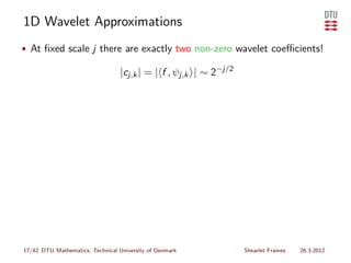
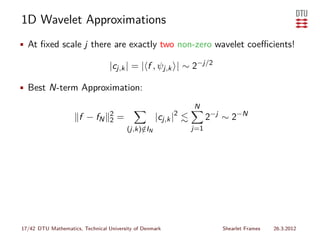
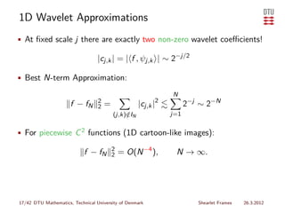
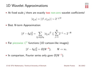
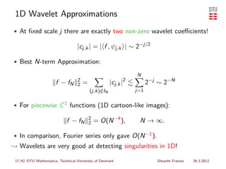
![1D Wavelet Approximations
• The wavelet system generated by ψ ∈ L2 (R) is
ψj,m = Dj Tm ψ = 2j/2 ψ(2j · −m) : j ∈ Z, m ∈ Z .
• ONB e.g., Haar Wavelet:
1 1
x ∈ [0, 2 ),
ψ(x) = −1 x ∈ [ 1 , 1),
2
0
otherwise.
• Haar Scaling function Tm φ, m ∈ Z (replaces ψj,m , j < 0, m ∈ Z):
φ(x) = χ[0,1] (x)
16/42 DTU Mathematics, Technical University of Denmark Shearlet Frames 26.3.2012](https://image.slidesharecdn.com/shearlet3dpresentation-120326034830-phpapp01/85/Shearlet-Frames-and-Optimally-Sparse-Approximations-25-320.jpg)


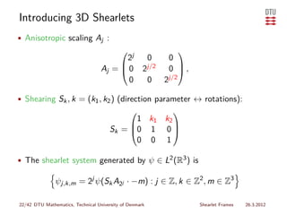
![Introducing 3D Shearlets
• Anisotropic scaling Aj (α ∈ (1, 2]):
2jα/2 0 0
Aj = 0 2j/2 0 ,
0 0 2j/2
• Shearing Sk , k = (k1 , k2 ) (direction parameter ↔ rotations):
1 k1 k2
Sk = 0 1 0
0 0 1
• The shearlet system generated by ψ ∈ L2 (R3 ) is
1
ψj,k,m = 2j( 4 + 2 ) ψ(Sk A2j · −m) : j ∈ Z, k ∈ Z2 , m ∈ Z3
α
22/42 DTU Mathematics, Technical University of Denmark Shearlet Frames 26.3.2012](https://image.slidesharecdn.com/shearlet3dpresentation-120326034830-phpapp01/85/Shearlet-Frames-and-Optimally-Sparse-Approximations-44-320.jpg)
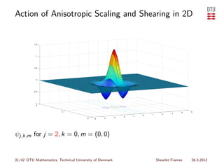
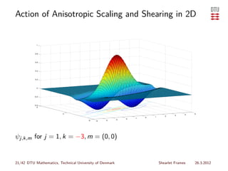
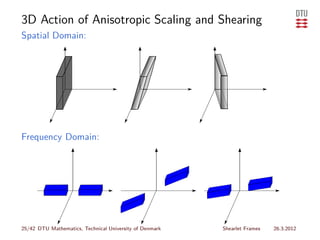
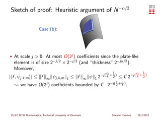
![Example: 3D Action of Anisotropic scaling and
Shearing
Example: Suppose supp ψ = [0, 1]3 . Let the translation parameter
m = (0, 0, 0) be fixed.
Scaling For k = (0, 0):
supp ψj,0,0 = [0, 2−j ] × [0, 2−j/2 ] × [0, 2−j/2 ] → the
shearlet becomes a small, plate-like element as j → ∞.
24/42 DTU Mathematics, Technical University of Denmark Shearlet Frames 26.3.2012](https://image.slidesharecdn.com/shearlet3dpresentation-120326034830-phpapp01/85/Shearlet-Frames-and-Optimally-Sparse-Approximations-46-320.jpg)
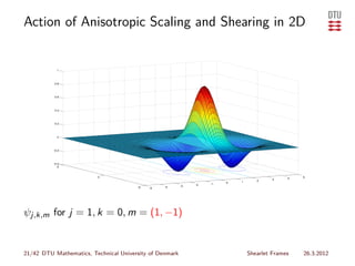
![Example: 3D Action of Anisotropic scaling and
Shearing
Example: Suppose supp ψ = [0, 1]3 . Let the translation parameter
m = (0, 0, 0) be fixed.
Scaling For k = (0, 0):
supp ψj,0,0 = [0, 2−j ] × [0, 2−j/2 ] × [0, 2−j/2 ] → the
shearlet becomes a small, plate-like element as j → ∞.
Shearing For j > 0: ψ(Sk A2j x) =
ψ(2j x1 + k1 2j/2 x2 + k2 2j/2 x3 , 2j/2 x2 , 2j/2 x3 )
24/42 DTU Mathematics, Technical University of Denmark Shearlet Frames 26.3.2012](https://image.slidesharecdn.com/shearlet3dpresentation-120326034830-phpapp01/85/Shearlet-Frames-and-Optimally-Sparse-Approximations-47-320.jpg)
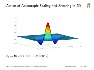
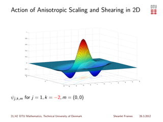
![Example: 3D Action of Anisotropic scaling and
Shearing
Example: Suppose supp ψ = [0, 1]3 . Let the translation parameter
m = (0, 0, 0) be fixed.
Scaling For k = (0, 0):
supp ψj,0,0 = [0, 2−j ] × [0, 2−j/2 ] × [0, 2−j/2 ] → the
shearlet becomes a small, plate-like element as j → ∞.
Shearing For j > 0: ψ(Sk A2j x) =
ψ(2j x1 + k1 2j/2 x2 + k2 2j/2 x3 , 2j/2 x2 , 2j/2 x3 )
Problem To get horizontal plate-elements require very large
shear parameters |ki | = ∞ ❀ non-uniform treatment
of directions.
24/42 DTU Mathematics, Technical University of Denmark Shearlet Frames 26.3.2012](https://image.slidesharecdn.com/shearlet3dpresentation-120326034830-phpapp01/85/Shearlet-Frames-and-Optimally-Sparse-Approximations-48-320.jpg)
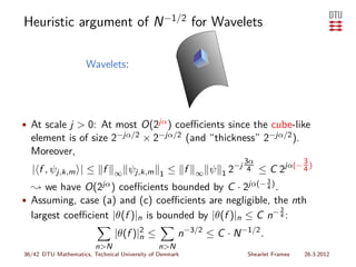
![Revisiting 3D Cartoon-like Images
Definition
2
Let 1 < α ≤ 2. The set of 3D images Eα (R3 ) is defined by
Eα (R3 ) = {f ∈ L2 (R3 ) : f = f0 +f1 χB } fi ∈ C 2 (R3 ), supp fi ⊂ [0, 1]3 ,
2
where B ⊂ [0, 1]3 and the boundary surface ∂B is a closed
C α -surface with ‘curvature’ bounded by ν.
❇➯
✶
✺✼ ✳✵
✵✺ ✳✵
✺✷✳✵
✶
✺✼✳✵
✵
✵ ✵✺ ✳✵
✺✷ ✳✵
✵✺✳✵ ✺✷✳✵
✺✼ ✳✵
✵
✶
29/42 DTU Mathematics, Technical University of Denmark Shearlet Frames 26.3.2012](https://image.slidesharecdn.com/shearlet3dpresentation-120326034830-phpapp01/85/Shearlet-Frames-and-Optimally-Sparse-Approximations-54-320.jpg)
![Revisiting 3D Cartoon-like Images
Definition
Let 1 < α ≤ 2. The set of 3D images Eα (R3 ) is defined by
2
Eα (R3 ) = {f ∈ L2 (R3 ) : f = f0 +f1 χB } fi ∈ C 2 (R3 ), supp fi ⊂ [0, 1]3 ,
2
where B ⊂ [0, 1]3 and the boundary surface ∂B is a closed
C α -surface with ‘curvature’ bounded by ν.
Theorem (Kutyniok, L, Lim; 2011)
Let (ψλ )λ ⊂ L2 (R3 ). The optimal asymptotic approximation error
of f ∈ Eα (R3 ) is
2
2
f − fN 2 N −α/2 , N → ∞, where fN = cλ ψλ .
λ∈IN
29/42 DTU Mathematics, Technical University of Denmark Shearlet Frames 26.3.2012](https://image.slidesharecdn.com/shearlet3dpresentation-120326034830-phpapp01/85/Shearlet-Frames-and-Optimally-Sparse-Approximations-55-320.jpg)
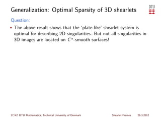
![Main result: Optimal Sparsity of 3D shearlet
Theorem (Kutyniok, L, Lim; 2011)
˜ ˘
Fix α ∈ (1, 2]. Let φ, ψ, ψ, ψ ∈ L2 (R3 ) be compactly supported.
Assume:
ˆ
(i) |ψ(ξ)| min(1, |ξ1 |δ ) · 3 min(1, |ξi |−γ )
i=1
∂ ˆ |ξ2 | −γ |ξ3 | −γ
(ii) ∂ξi ψ(ξ) ≤ |h(ξ1 )| · 1 + |ξ1 | 1+ |ξ1 | , i = 2, 3,
˜ ˘
where δ > 8, γ ≥ 4, h ∈ L1 (R), and similar for ψ and ψ. Further,
˜ ψ; α) forms a frame for L2 (R3 ). For
suppose that SH(φ, ψ, ψ, ˘
f ∈ Eα (R3 ),
2
2 O(N −α/2+µ ), if α < 2,
f − fN 2 = −1 2
as N → ∞,
O(N (log N) ), if α = 2,
where 3(2−α)(α−1)(α+2)
µ = µ(α) = 2(9α2 +17α−10)
,
30/42 DTU Mathematics, Technical University of Denmark Shearlet Frames 26.3.2012](https://image.slidesharecdn.com/shearlet3dpresentation-120326034830-phpapp01/85/Shearlet-Frames-and-Optimally-Sparse-Approximations-56-320.jpg)


The document discusses shearlet frames and their application in optimally sparse approximations within the context of applied harmonic analysis and imaging sciences. It highlights the importance of capturing anisotropic features in both 2D and 3D data for tasks such as denoising and feature extraction. The aim is to establish a representation system for 3D data that matches the effectiveness of wavelets for 1D data.