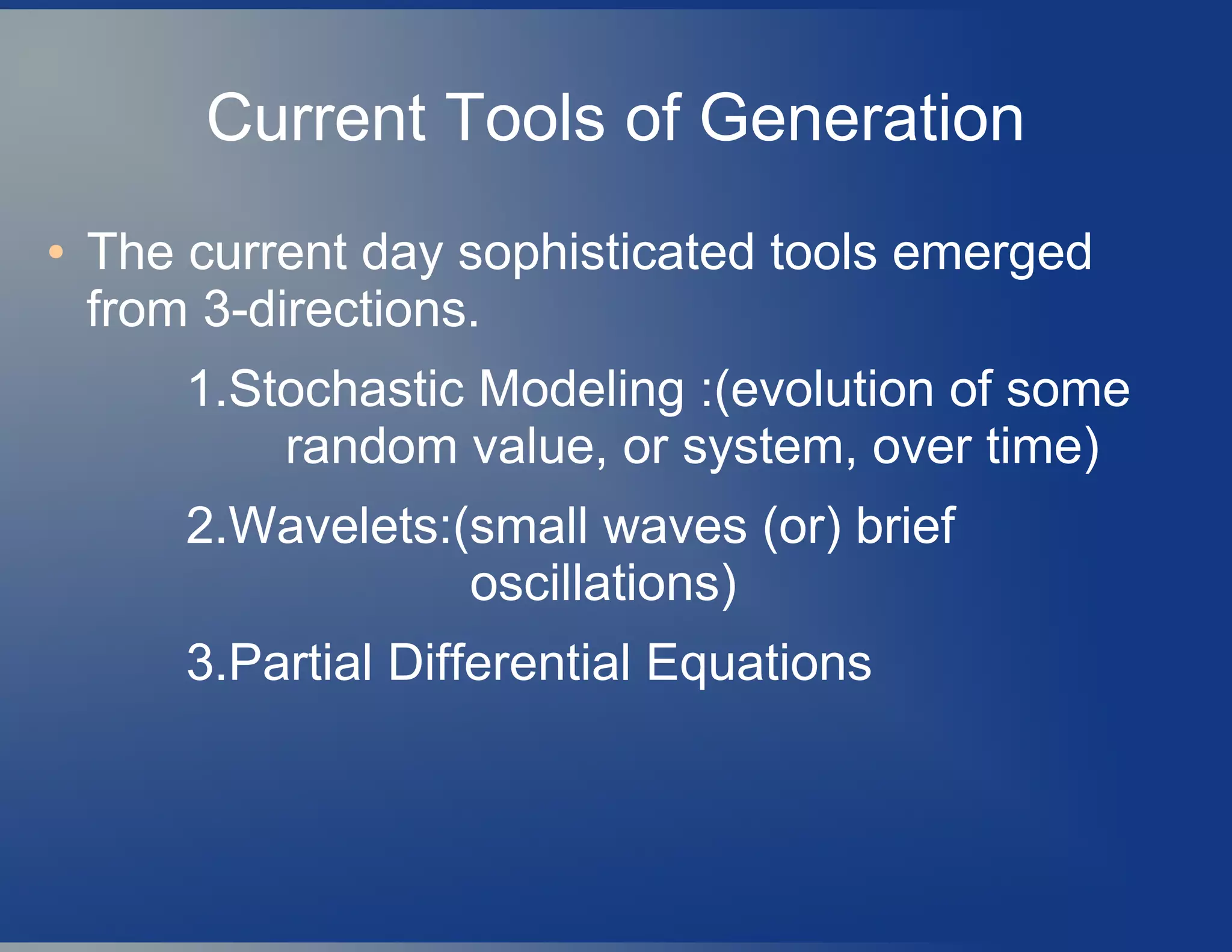
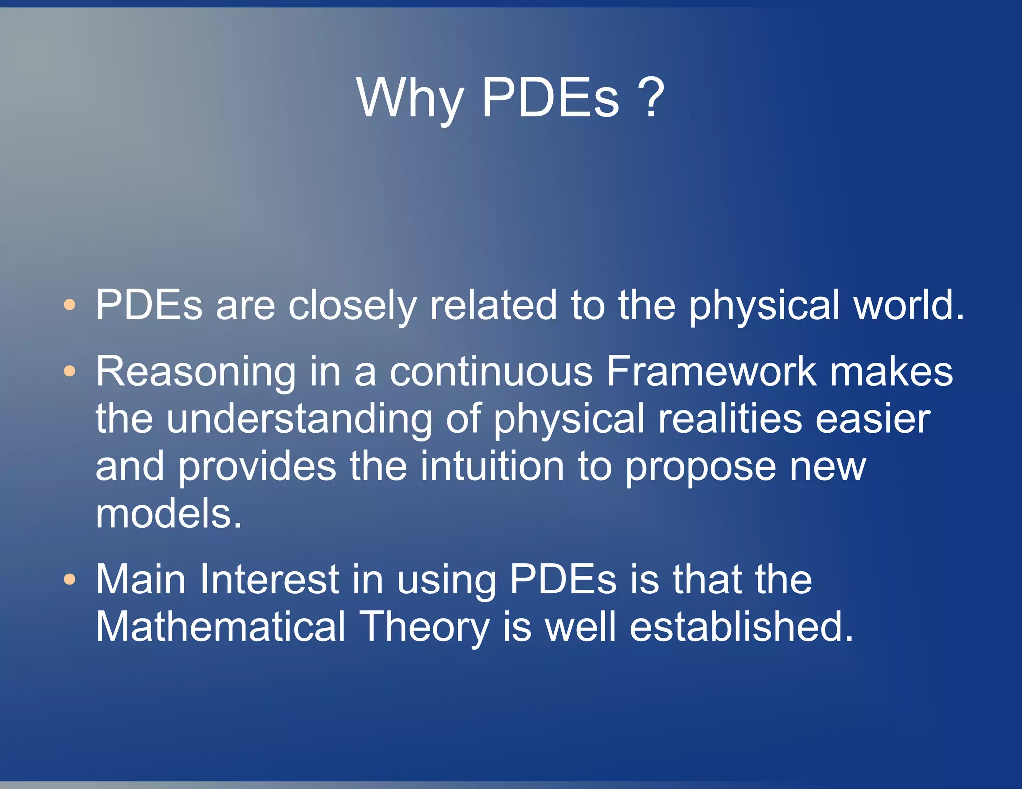
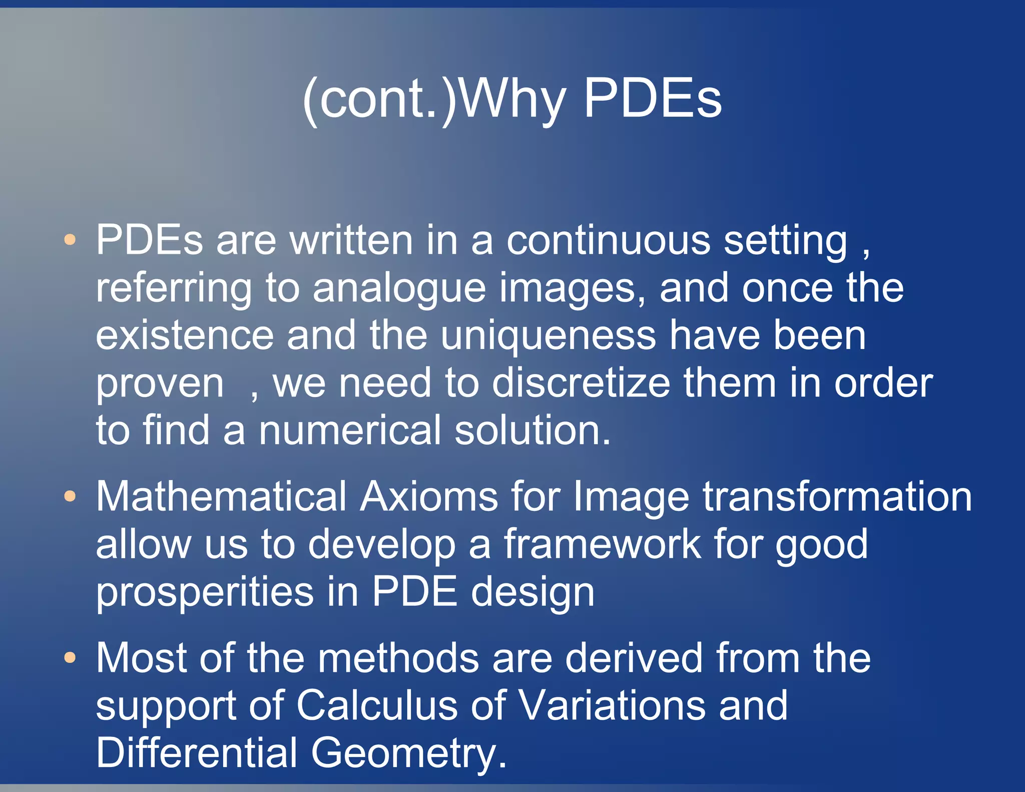
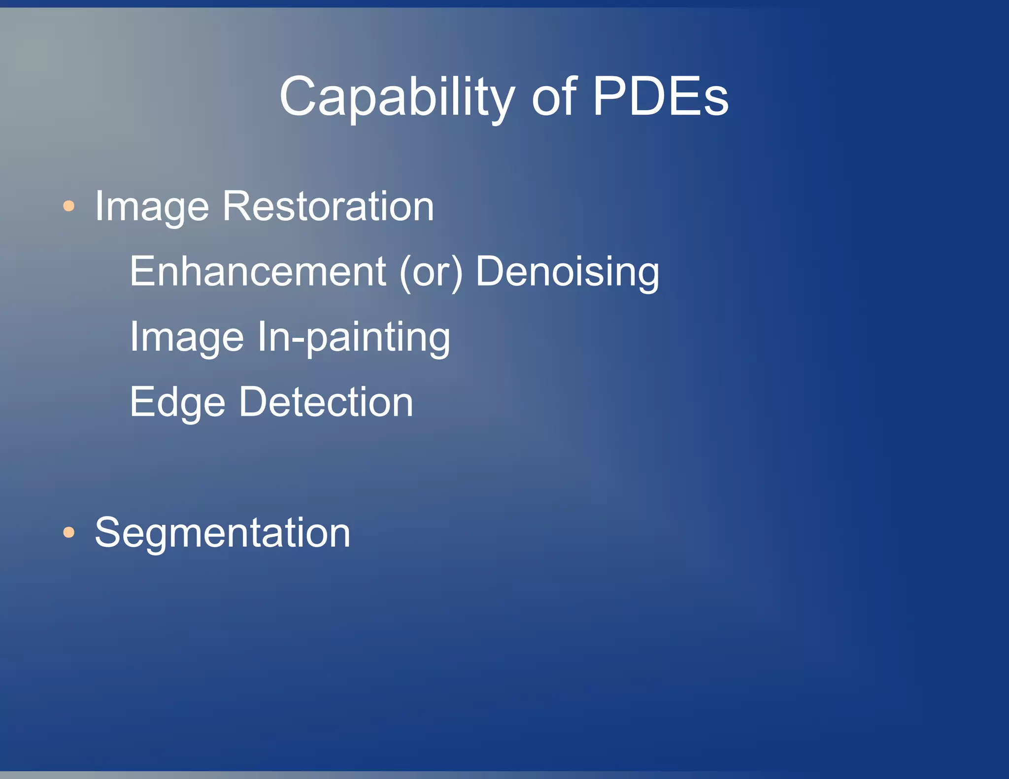
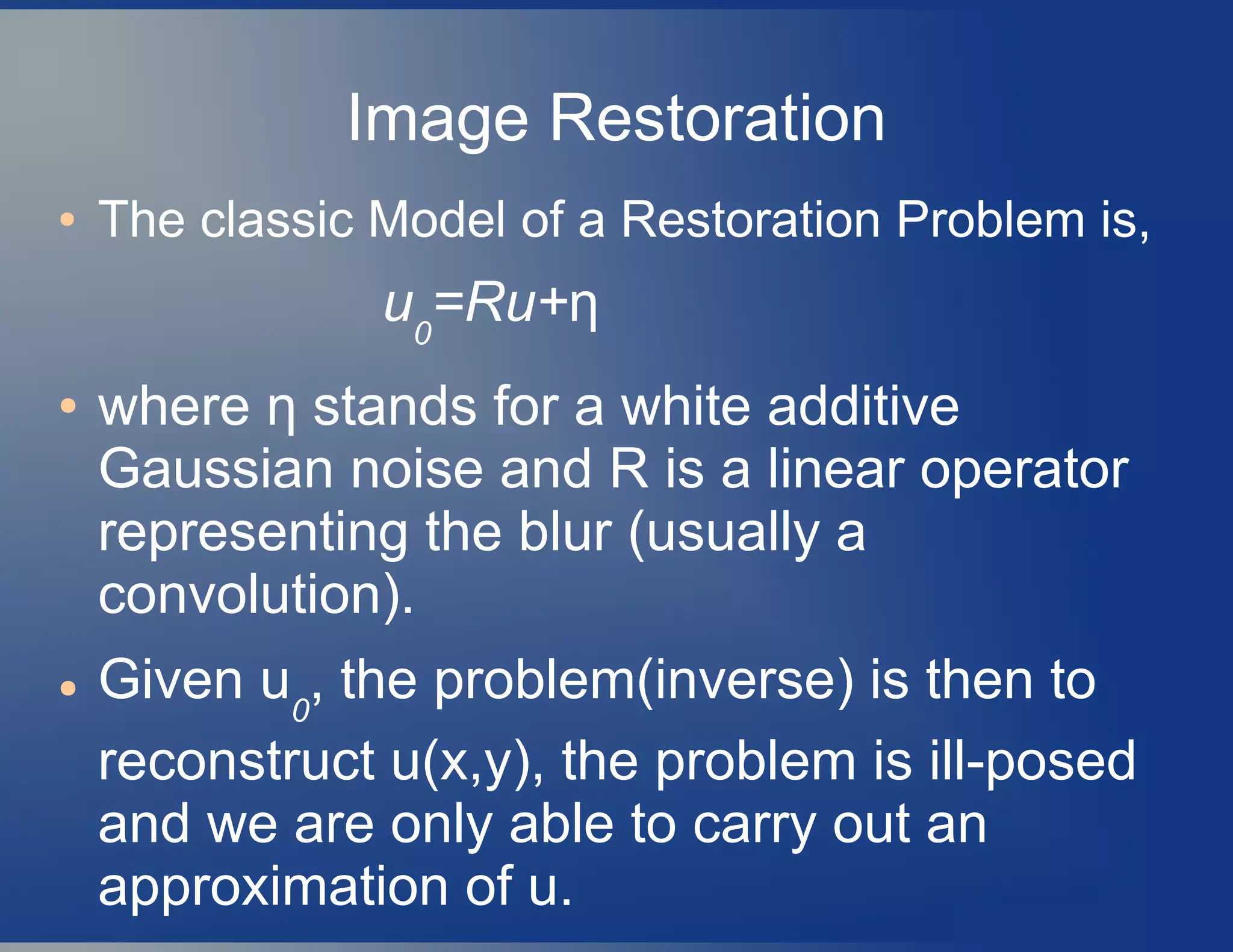
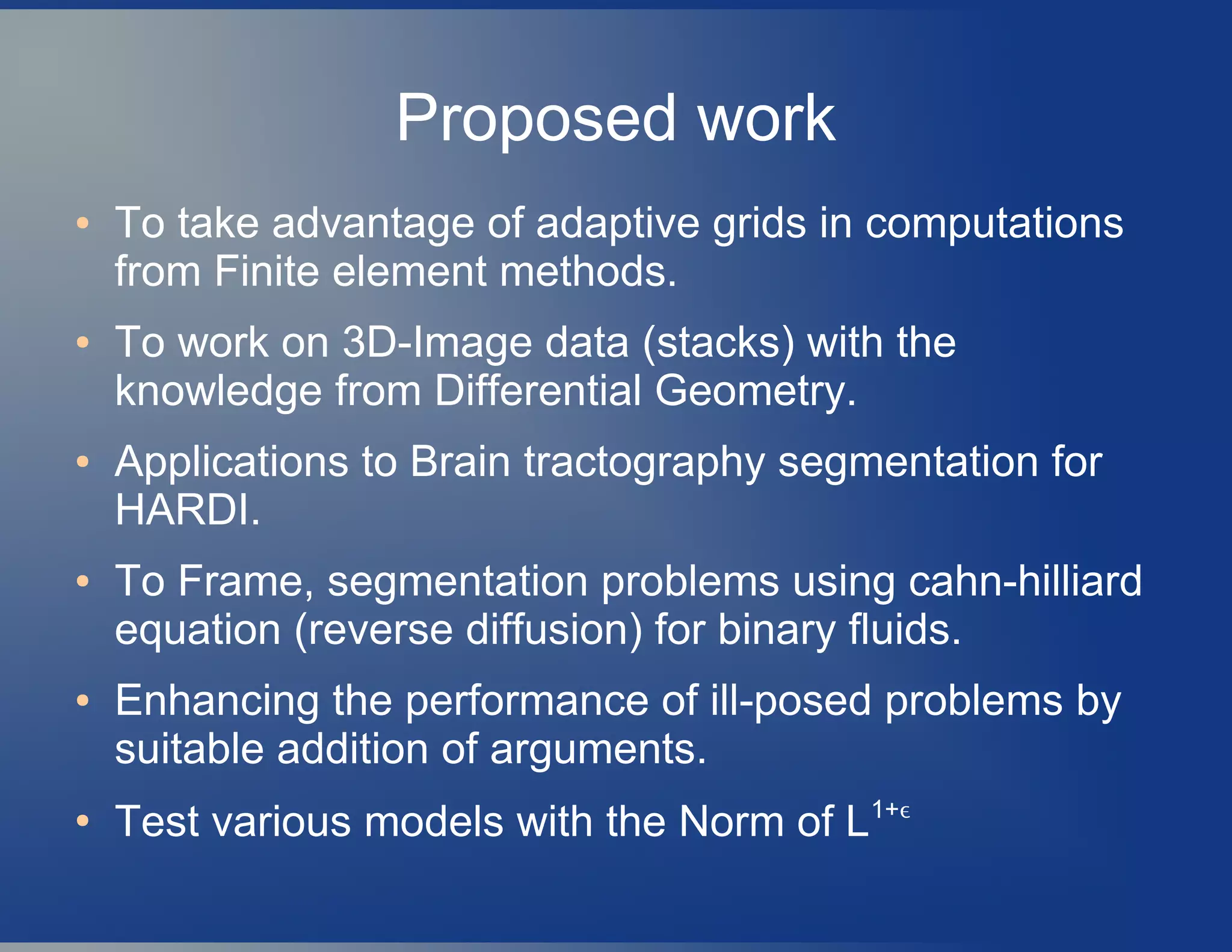
State of art pde based ip to bt vijayakrishna rowthu

A State of Art Seminar
on
Variational P.D.E. based Image
Processing with
Applications to HDBT
Vijayakrishna Rowthu
(Y9108070)
Under the guidance of
Prof.B.V.Rathish Kumar
Dept. of Mathematics & Statistics

contents
● What is an Image?
● Defects in Images and Recovery
● PDEs in Image Processing
● Variational/PDE Models from Axioms and
Results
● DTI and Brain Fibre Tracking
● Existing Methods and comparison
● Proposed work
● References

What is an Image?
● An Image is a 2-D
view (projection in a
specific direction ) of
the surface of an
object (or a scene)
from the space we
live-in(3D) that is
formed by the light
rays reflected by the
object.

Basics of an Image
● Analogue Image(Continuous Image):
● Digital Image(Discrete Image): Obtained from
an analogue Image by sampling and
quantization.
--- Represented as A 2-Dimensional array
of pixels with assigned brightness values.
● Resolution: The number of Rows and
Columns in an image.
● The higher the resolution , the closer the
digital image is to the physical world.

Mathematical Representation
Define an analogue Image(u) as a measurable
,bounded function:
Where Ω is a connected,bounded domain
from ℝ2
, And ℝd
is an intensity valued Range set.
In case of A Digital(Discrete) Image(I ):
For Grey Images : d=1 ; RGB images :d=3

Digital Image Processing
● Image processing is a Mathematical
procedure involving computer algorithms
where the input is an image ,And , the output
may be either an image or a set of
characteristics or parameters related to the
image.
● Most image-processing techniques involve
treating the image as a two-dimensional signal
and applying standard signal-processing
techniques to it.

Some Rough Idea on Edges
● Typically, an Image represents a scene
containing a background and several objects.
● It is common that , inside the background and
in each object the values are smoothly
varying, but are discontinuous or change
abruptly across object boundaries (edges),
thus creating large image gradients at these
locations.
● We define edges as the locations where the
gradient | f| is large due to a discontinuity or∇
a sharp transition in the image intensity.

Common Problems and
Known Remedies
● Noise (Unwanted information) , is a defect,
occurs during the recording & communication
process.
Local Averaging is a simple solution.
Local Median for impulse noise.
● Components Extraction(Segmentation):
By Properly detecting the contours (edge
sets) , one can achieve this goal, but the
contour finding in-general is not an easy task.

(cont.)Common Problems and
Known Remedies
● Deconvolution for Restoration, :
Restoration attempts to reconstruct or
recover an image that has been degraded by
using a priori knowledge of the degradation
phenomenon.
g(x,y)=H(f(x,y))+n(x,y)
● The main Difficulty arises when the SNR is
low.The results are highly sensitive to noise
,sometimes losing the basic Structure of the
image , even.
● The Least Square Error Filter(wiener) is a popular
Solution

Drawbacks
● It is difficult to say which one is more natural
approach than the other.
They rely on
–Filters
–Spectral Analysis
–Basic Concepts of Statistics & Probability

Image Processor
● Abstractly, image processing can be
considered as an input-output system
Q0
→ Image Processor T → Q
● The input data Q0
can represent an observed
single image , and the output Q = (q1,q2,···)
contains all the targeted image features.
● Typical image processors(T):
denoising,deblurring,segmentation,
compression, or inpainting.

Models of Some Image Processors

Current Tools of Generation
● The current day sophisticated tools emerged
from 3-directions.
1.Stochastic Modeling :(evolution of some
random value, or system, over time)
2.Wavelets:(small waves (or) brief
oscillations)
3.Partial Differential Equations

Why PDEs ?
● PDEs are closely related to the physical world.
● Reasoning in a continuous Framework makes
the understanding of physical realities easier
and provides the intuition to propose new
models.
● Main Interest in using PDEs is that the
Mathematical Theory is well established.

(cont.)Why PDEs
● PDEs are written in a continuous setting ,
referring to analogue images, and once the
existence and the uniqueness have been
proven , we need to discretize them in order
to find a numerical solution.
● Mathematical Axioms for Image transformation
allow us to develop a framework for good
prosperities in PDE design
● Most of the methods are derived from the
support of Calculus of Variations and
Differential Geometry.

Capability of PDEs
● Image Restoration
Enhancement (or) Denoising
Image In-painting
Edge Detection
● Segmentation

In computer Vision ,analyzing images at different resolutions(scale)
is necessary to extract Various Descriptions of an Image.
As a primitive scale-parametrization, the Gaussian convolution is
attractive for its "well-behavedness":
● The Gaussian is symmetric and strictly decreasing about the
mean, and therefore the weighting assigned to signal values
decreases smoothly with distance.
● The Gaussian convolution behaves well near the limits of the
scale parameter, t,
approaching the un-smoothed Image for small t, and
approaching the Mean value of Image for large t.
● The Gaussian is also readily differentiated and integrated.
Gaussian Smoothing[witkin]

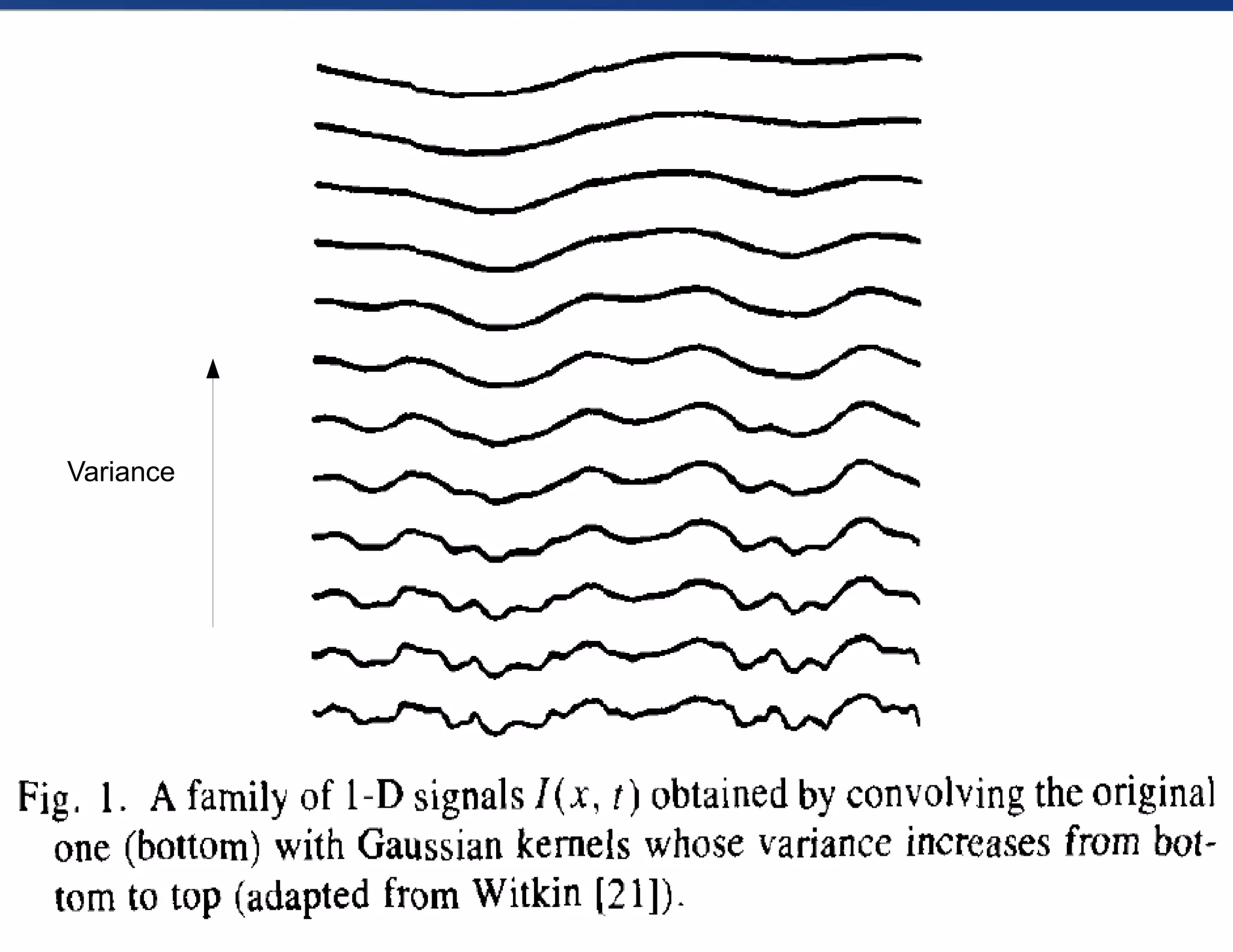
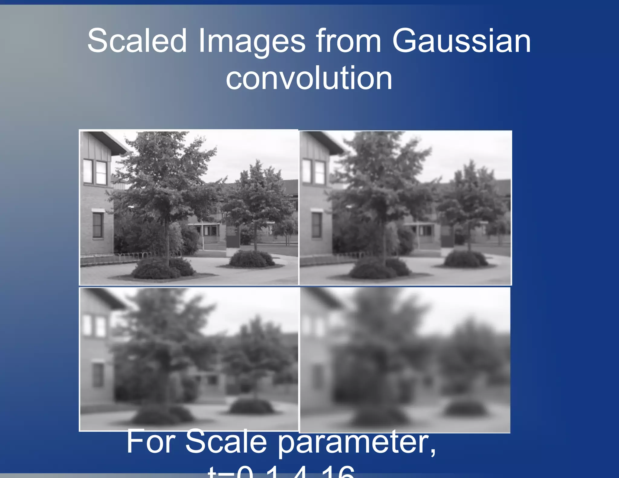
The first step in this direction is Scale
Space Filtering for Smoothing
● [Witkin,1983]:(Scale Space)
The essential idea of this approach is to,
Embed the original image in a family of derived
images { I(x, y, t);t≥0} obtained by convolving
the original image I0
(x,y) with a Gaussian kernel
G(x,y; t) of variance t.
I(x,y,t) = I0
(x, y)*G(x,y;t)
● Larger values of t (the scale-space parameter),
correspond to images at coarser resolutions.

Scaled Images from Gaussian
convolution
For Scale parameter,

Scale-Space
Define a multi-scale analysis(Scale
Space)as a family of operators {Tt
;t ≥ 0}
which, applied to the original image u0
(x), yield
to a sequence of images
u(t,x) = (Tt
u0
)(x)
For simplicity, we suppose for all t ≥ 0,
Tt
: C∞
b
(R2
) → Cb
(R2
) where C∞
b
(R2
) is the
space of bounded functions having
derivatives at any order.

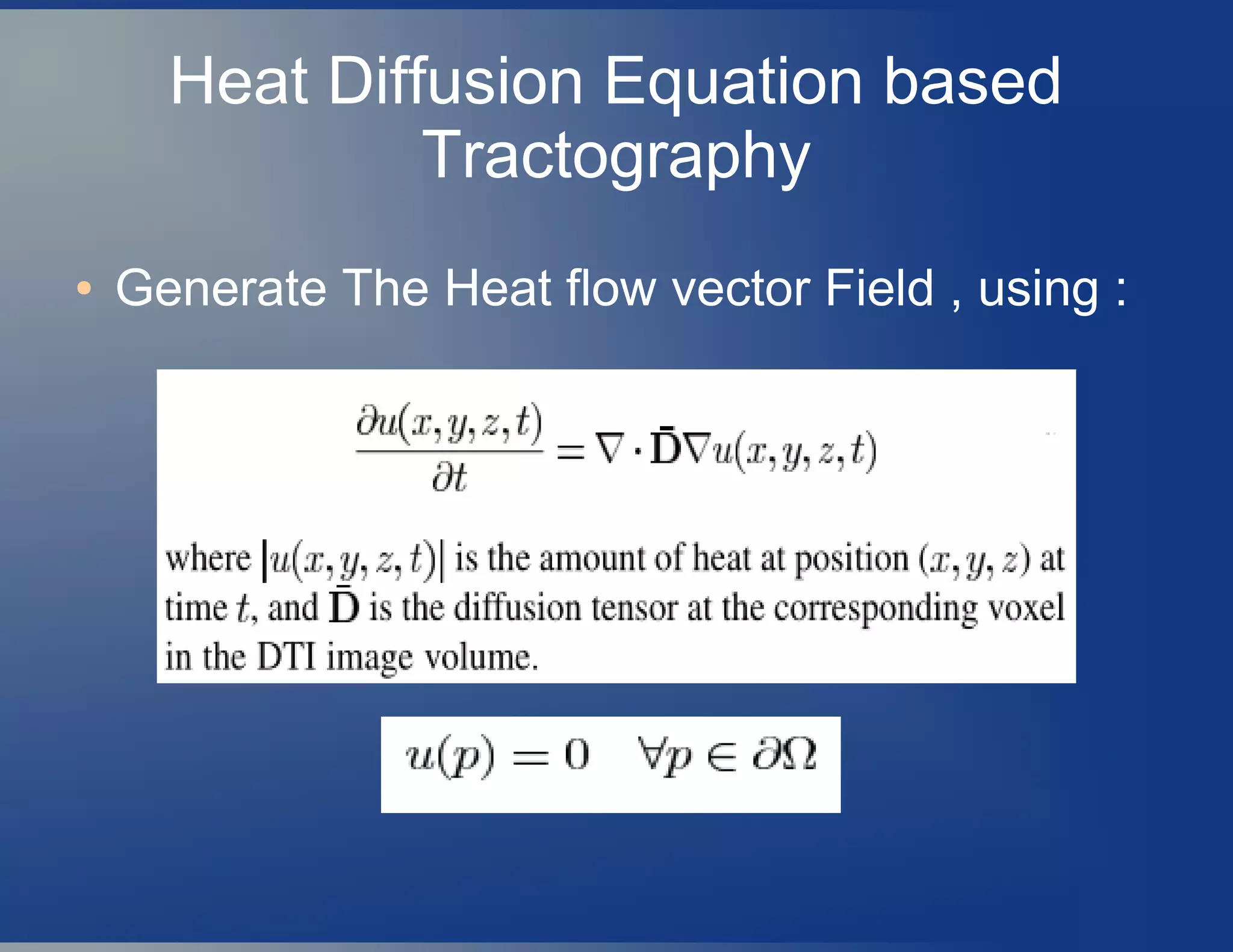
Relating to the Heat Diffusion
Equation (Linear Diffusion)
[Koenderink and Hummel ]:
These one parameter family of derived (scale-
space) images may equivalently be viewed as the
solution of the heat diffusion equation.
It
=ΔI =Ixx
+Iyy
(Isotropic Diffusion)
with the initial condition,
I(x,y,0)=I0
(x, y), the original image and
with no intensity loss at boundaries.

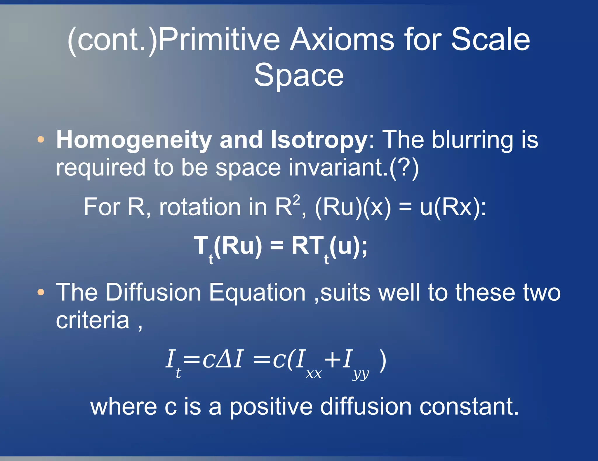
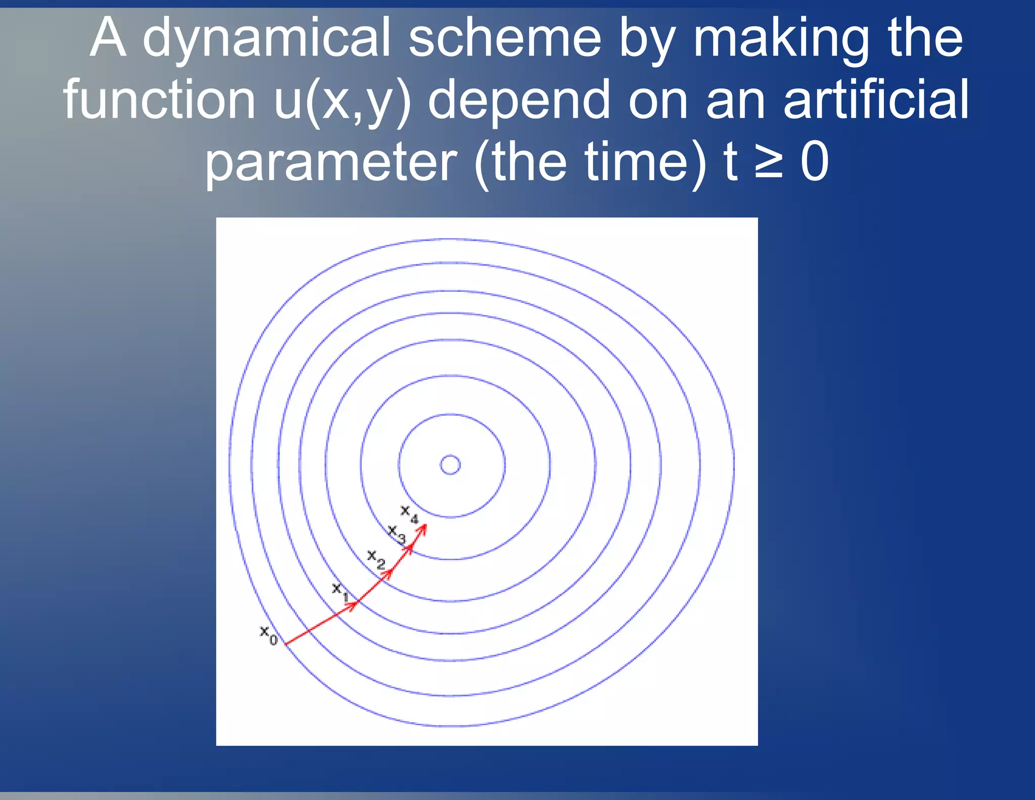
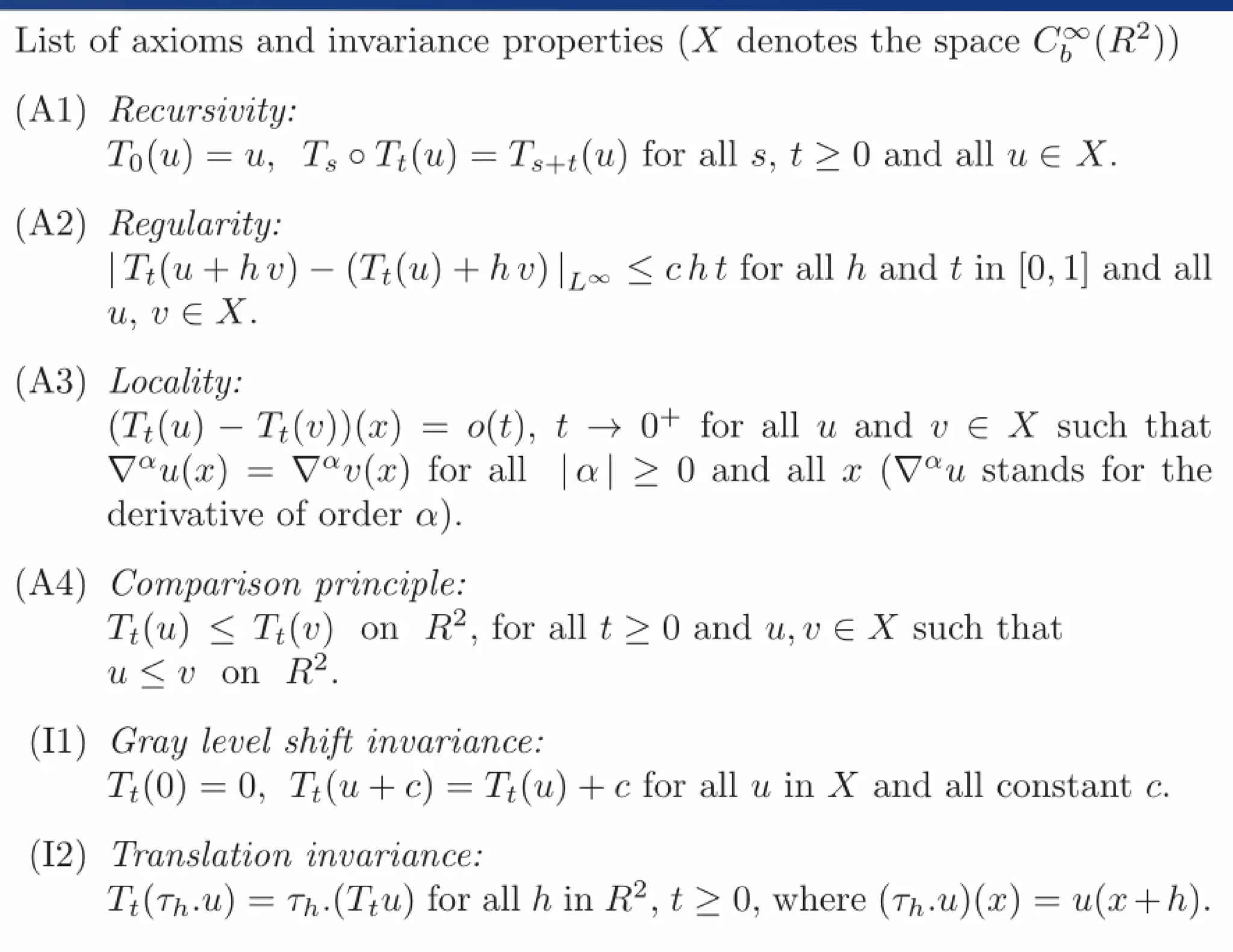
Primitive Axioms for Scale
Space(Linear Filters)
[Koenderink] motivates the diffusion equation
formulation by stating two criteria.
● 1) Causality: Any feature at a coarse level of
resolution is required to possess a (not
necessarily unique) “cause” at a finer level of
resolution although the reverse need not be
true.
i.e. no spurious detail should be generated
when the resolution is diminished.
T0
= Id and s < t, T∀ ∃ (s,t)
: Tt
= T(s,t)
◦ Ts
;

(cont.)Primitive Axioms for Scale
Space
● Homogeneity and Isotropy: The blurring is
required to be space invariant.(?)
For R, rotation in R2
, (Ru)(x) = u(Rx):
Tt
(Ru) = RTt
(u);
● The Diffusion Equation ,suits well to these two
criteria ,
It
=cΔI =c(Ixx
+Iyy
)
where c is a positive diffusion constant.

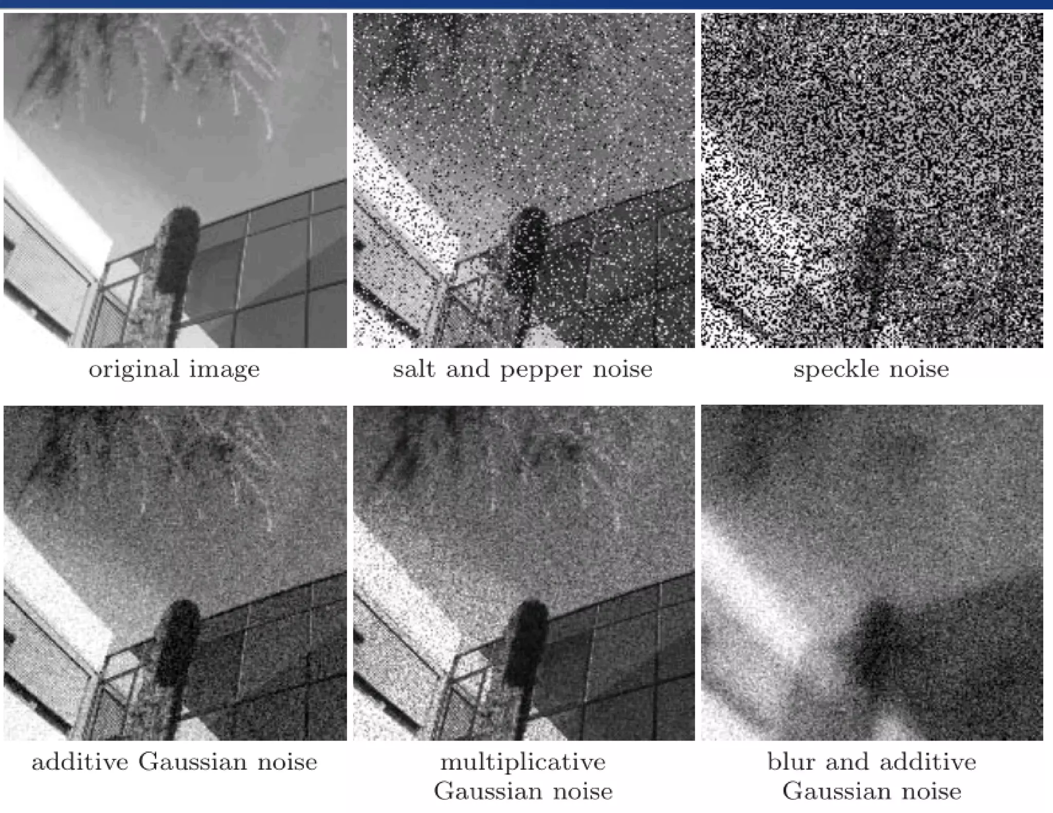
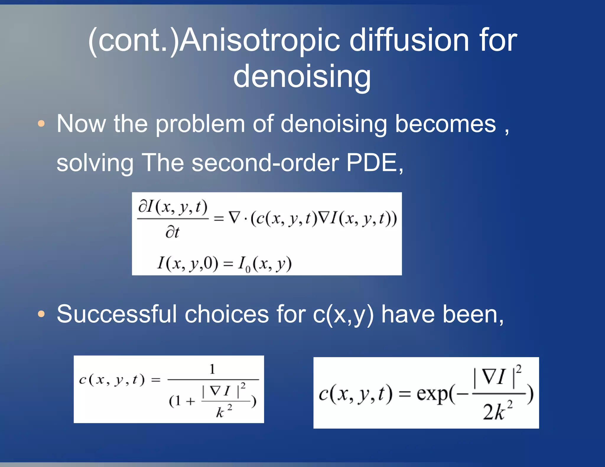
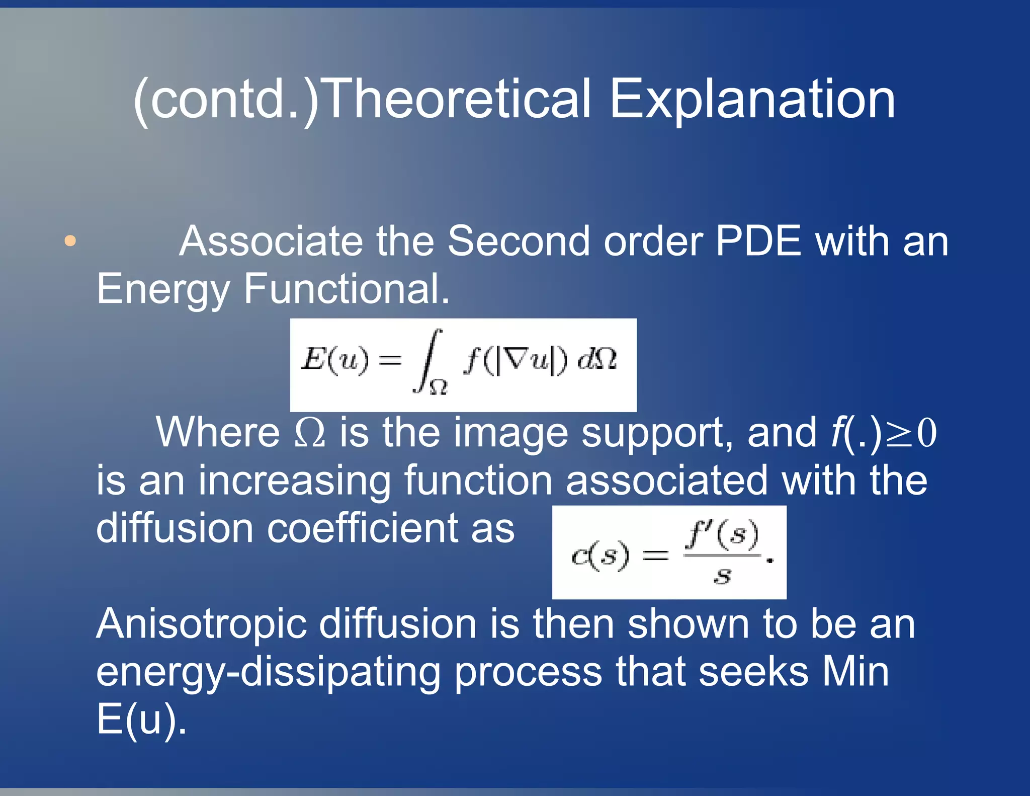
Anisotropic diffusion for denoising
● [Perona & Malik,1987]: Observed that
isotropic diffusion is causing a serious
damage to the visibility of Edges as diffusion
progresses.
● Found that , directionally dependent
smoothing is the right choice for preserving
edges with better Image denoising
(enhancement / smoothing).
● Chose, the diffusion factor c(x,y) ,in such a
way that the diffusion will be relatively faster at
locations of low Gradient than at the locations
of High Gradients(Edges).

(cont.)Anisotropic diffusion for
denoising
● Now the problem of denoising becomes ,
solving The second-order PDE,
● Successful choices for c(x,y) have been,

(contd.)Theoretical Explanation
● Associate the Second order PDE with an
Energy Functional.
Where Ω is the image support, and f(.)≥0
is an increasing function associated with the
diffusion coefficient as
Anisotropic diffusion is then shown to be an
energy-dissipating process that seeks Min
E(u).

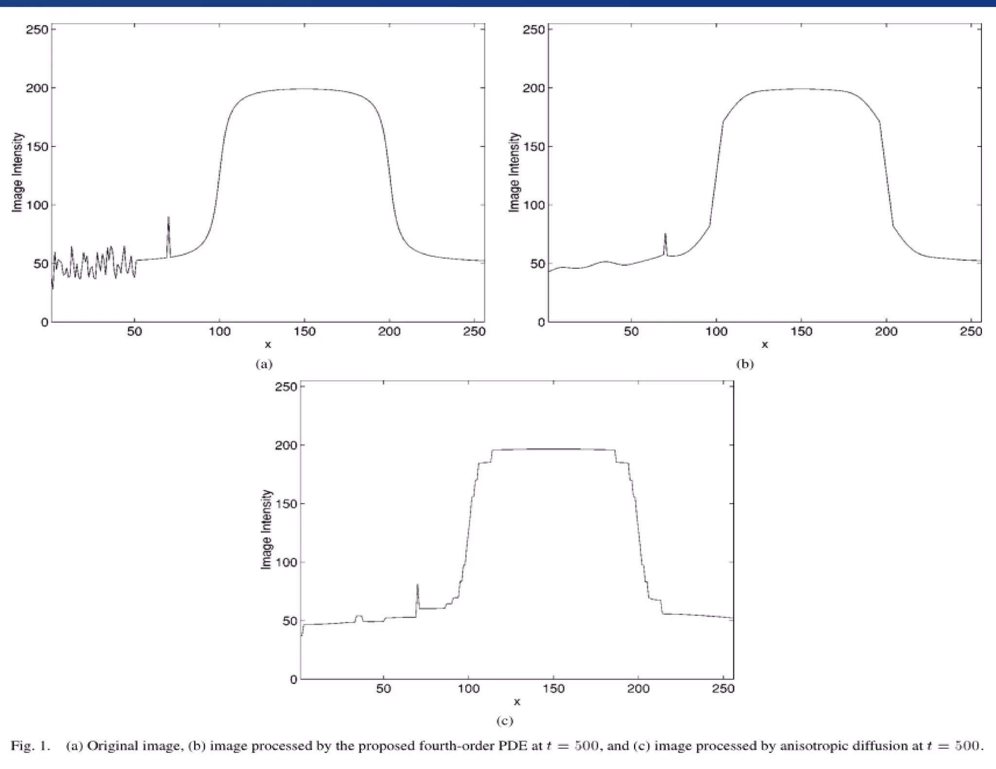
Flaws in second order
● [Whittaker]:
Since the Laplacian of an image at a pixel is zero if
the image is planar in its neighborhood, these PDEs
attempt to remove noise and preserve edges by
approximating an observed image with a piecewise
planar image.
● Piecewise planar images look more natural than step
images(blocky) which anisotropic diffusion uses to
approximate an observed image.
● This effect is visually unpleasant and is likely to cause
a computer vision system to falsely recognize as
edges the boundaries of different blocks that actually
belong to the same smooth area in the original image.

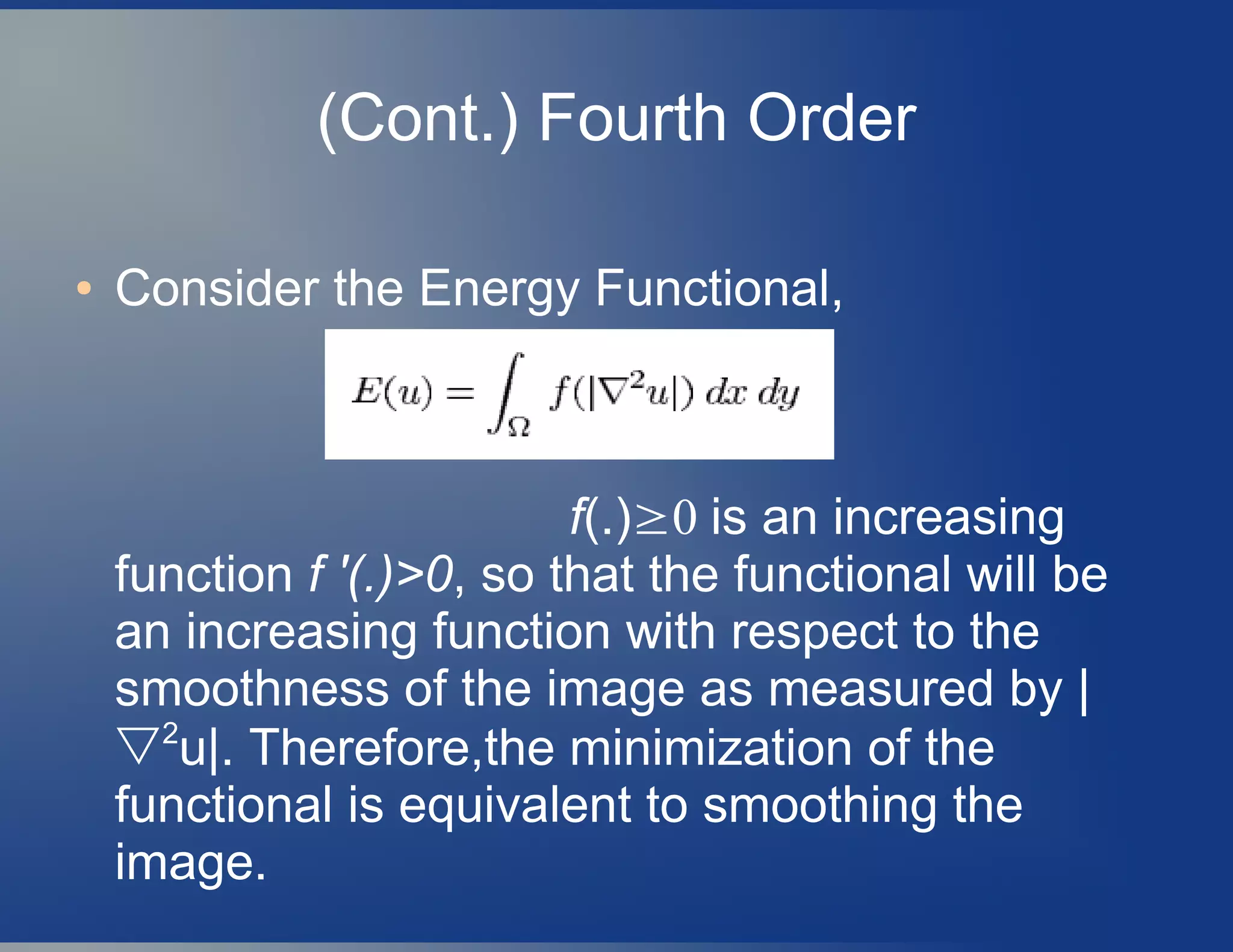
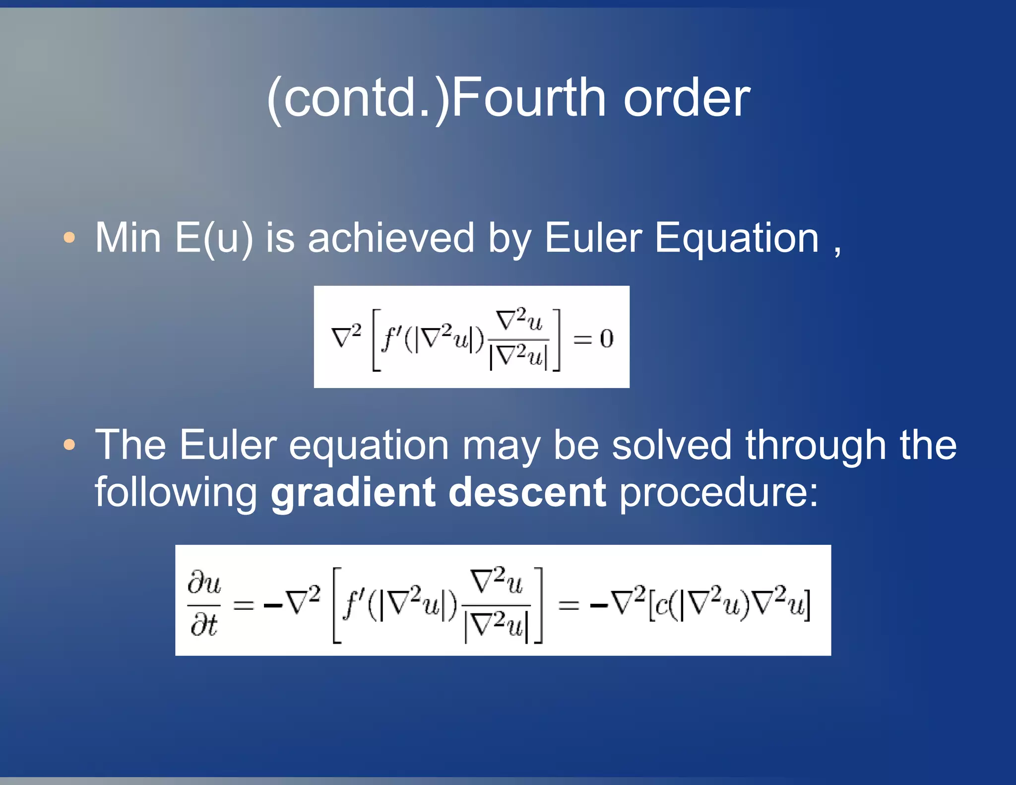
It's extensions to fourth order
● [You,Kaveh,2000]:
Fourth order linear diffusion dampens
oscillations at high frequencies much faster
than second order diffusion.
● To avoid blocky effects while achieving good
tradeoff between noise removal and edge
preservation.

(Cont.) Fourth Order
● Consider the Energy Functional,
f(.)≥0 is an increasing
function f '(.)>0, so that the functional will be
an increasing function with respect to the
smoothness of the image as measured by |
▽2
u|. Therefore,the minimization of the
functional is equivalent to smoothing the
image.

(contd.)Fourth order
● Min E(u) is achieved by Euler Equation ,
● The Euler equation may be solved through the
following gradient descent procedure:

A dynamical scheme by making the
function u(x,y) depend on an artificial
parameter (the time) t ≥ 0

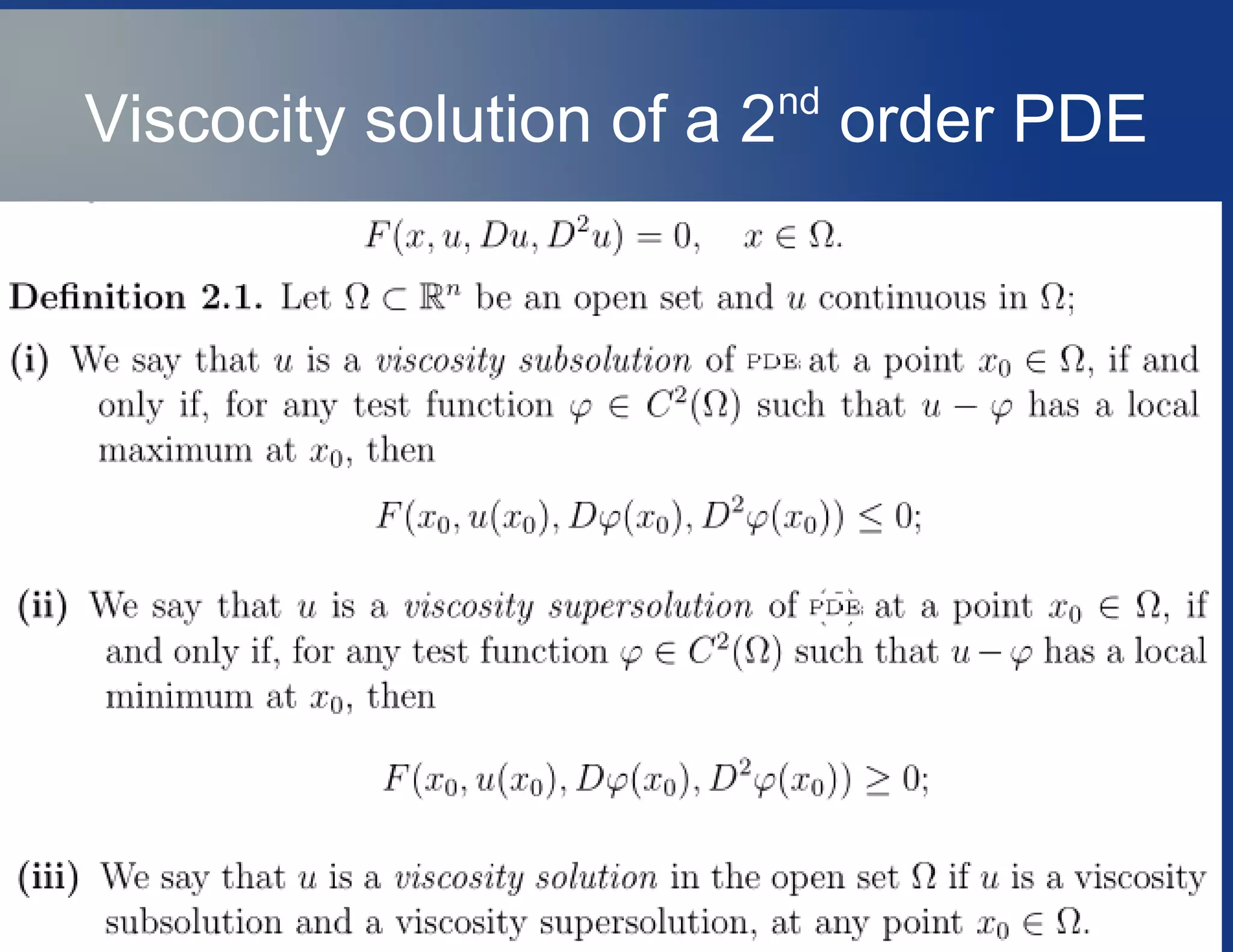
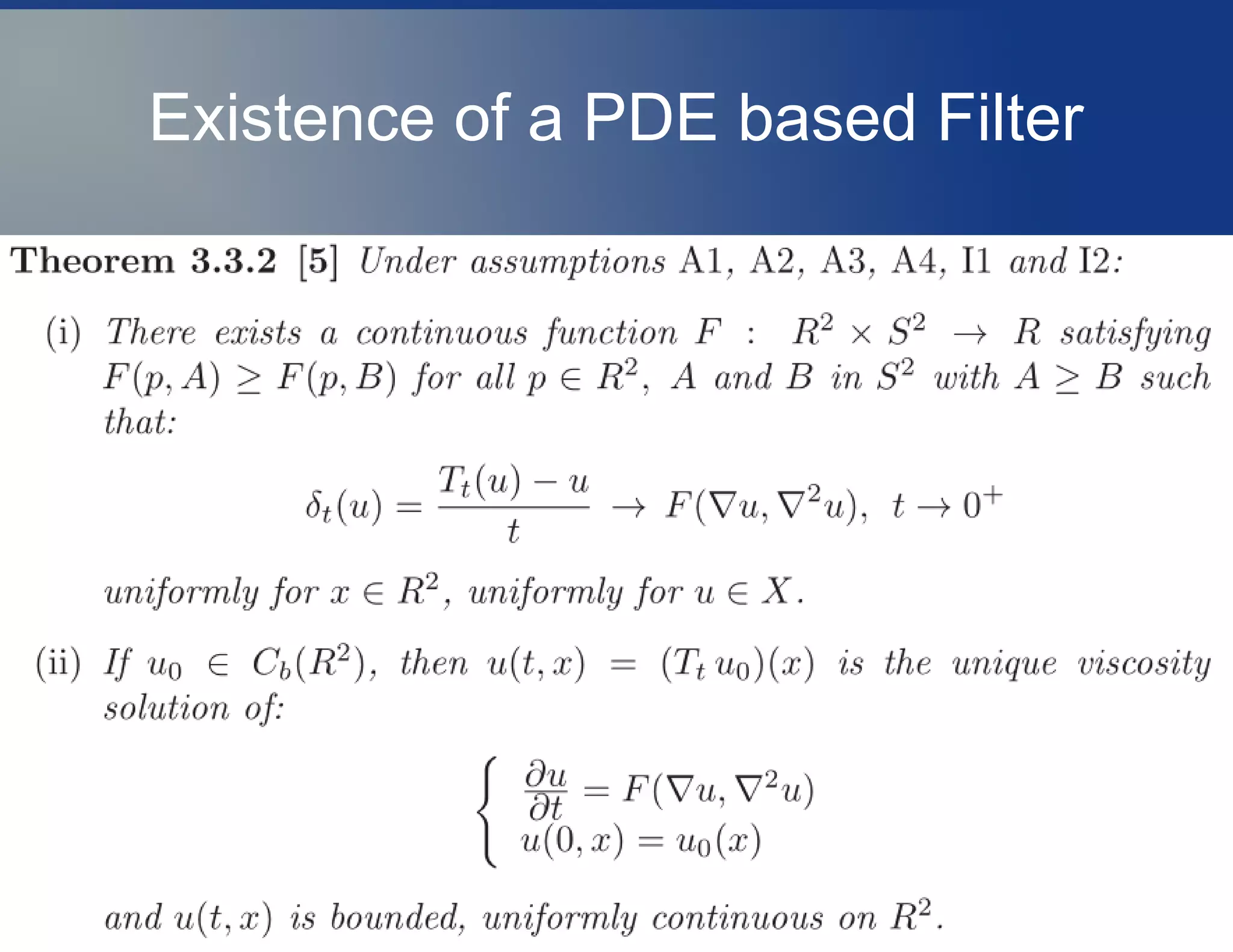
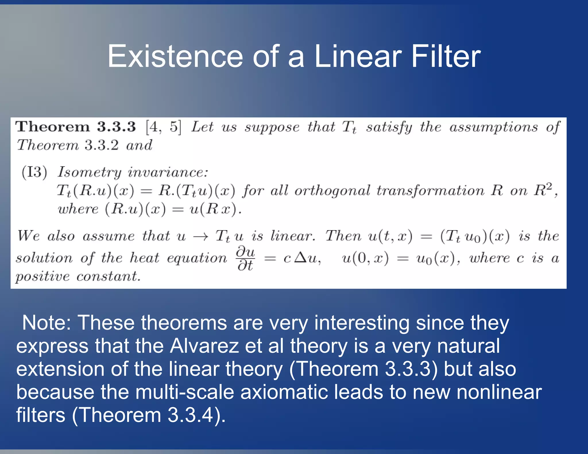
The Alvarez-Guichard-Lions-Morel
scale space theory
● The remarkable work of [Alvarez et al]
establishes the connection between scale
space analysis and PDEs , rigorously.
● Starting from a very natural filtering
axiomatic (based on desired image properties)
they prove that the resulting filtered image
must necessarily be the viscosity solution of a
PDE.
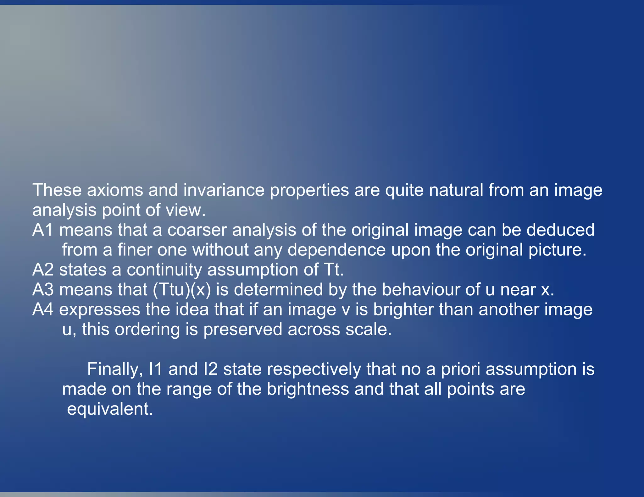
● Some Basic Axioms that are very natural from
Image Processing Perspective are:

Viscocity solution of a 2nd
order PDE

These axioms and invariance properties are quite natural from an image
analysis point of view.
A1 means that a coarser analysis of the original image can be deduced
from a finer one without any dependence upon the original picture.
A2 states a continuity assumption of Tt.
A3 means that (Ttu)(x) is determined by the behaviour of u near x.
A4 expresses the idea that if an image v is brighter than another image
u, this ordering is preserved across scale.
Finally, I1 and I2 state respectively that no a priori assumption is
made on the range of the brightness and that all points are
equivalent.

Classical definition concerning the
well-posedness of a
minimization problem or a PDE.
● Definition[Hadamard]:
When a minimization problem or a PDE
admit a unique solution which depends
continuously on the data, we say that the
minimization problem or the PDE are well-
posed.
● If one of the following conditions: existence,
uniqueness or continuity fails, we say that the
minimization problem or the PDE are ill-posed.

Existence of a PDE based Filter

Existence of a Linear Filter
Note: These theorems are very interesting since they
express that the Alvarez et al theory is a very natural
extension of the linear theory (Theorem 3.3.3) but also
because the multi-scale axiomatic leads to new nonlinear
filters (Theorem 3.3.4).

Curvature dependent Non-Linear
Filter

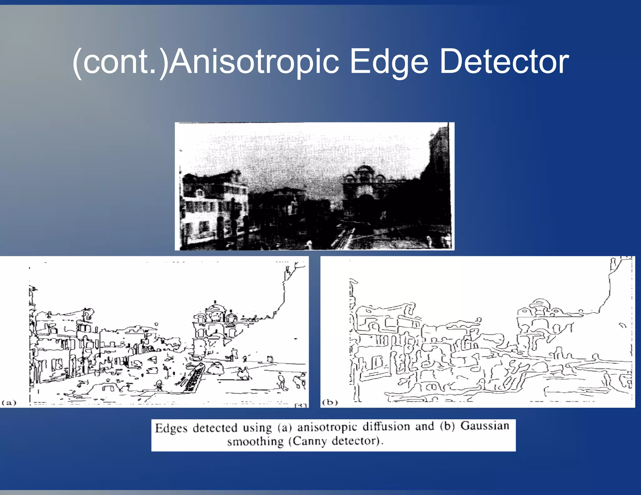
Edge-Detector from Anisotrpic
Diffusion[Perona & Malik]
● [Canny,1986] Edge Detector:The image is convolved
with the directional derivatives of a Gaussian.
u→ *▽( ( , ,σ))|u G x y |
Requires a number of convolutions ,involve
blurring And complexity of combining outputs of filters
at multiple scales.
● Anisotropic E.detector : The complication of multiple
scale, multiple orientation filters is avoided by locally
adaptive smoothing.
● In this, the edges are made sharp by the diffusion
process, so that edge thinning and linking are almost
unnecessary.

(cont.)Anisotropic Edge Detector

Image Restoration
● The classic Model of a Restoration Problem is,
u0
=Ru+η
● where η stands for a white additive
Gaussian noise and R is a linear operator
representing the blur (usually a
convolution).
● Given u0
, the problem(inverse) is then to
reconstruct u(x,y), the problem is ill-posed
and we are only able to carry out an
approximation of u.

The Energy Method
● supposing that η is a white Gaussian noise,
and according to the maximum likelihood
principle, to find an approximation of u by
solving the least square problem:
The Minimizer (if exists) satisfies the
equation,
● This is an ill-posed problem as, R*R is not
always one-to-one & may have small
eigenvalues.

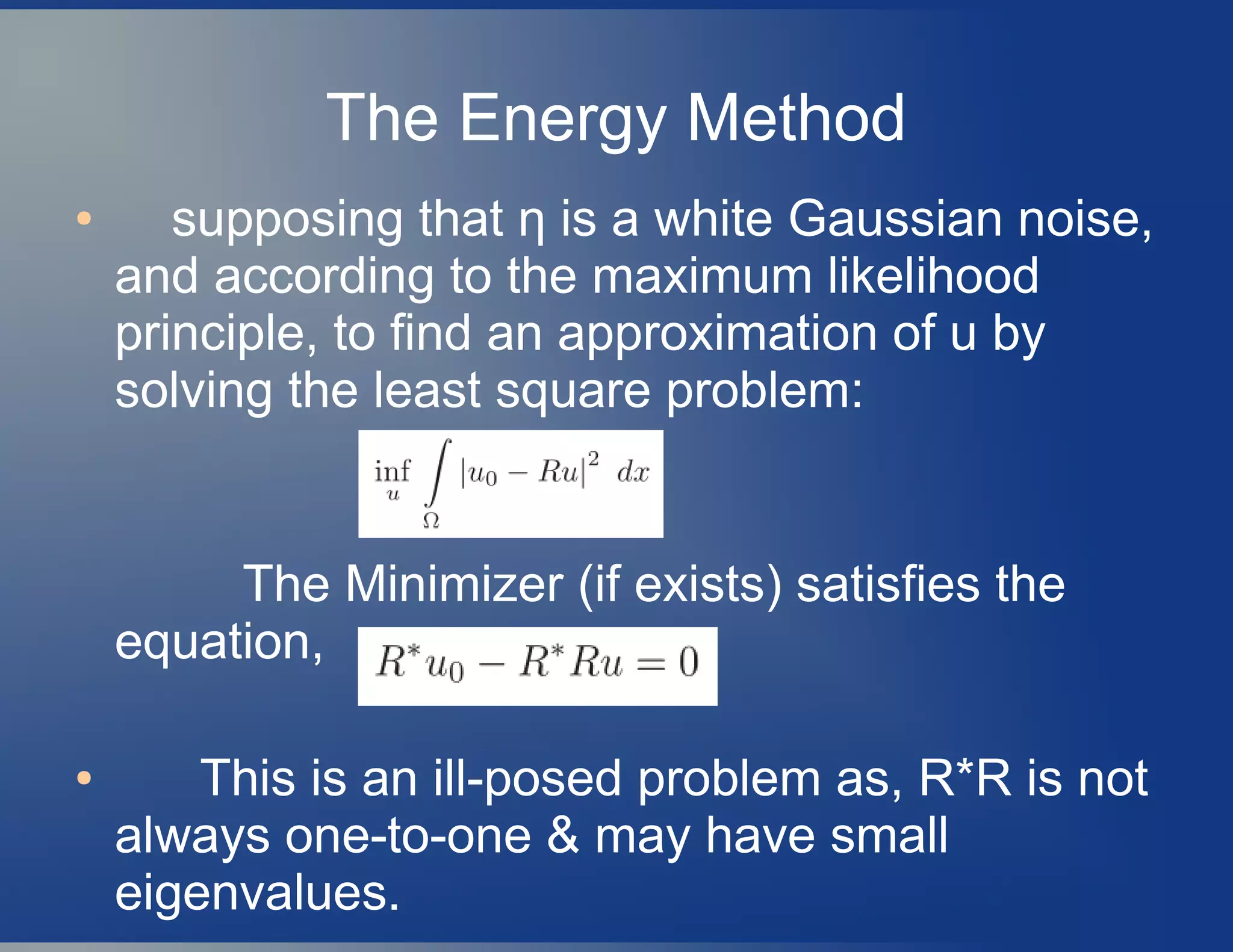
Regularisation of the problem(ill-
posed)
● [Tikhonov and Arsenin,1977]:(data fidelity+smoothing)
in Functional Space,
● Solution characterized by the Euler-Lagrange
equation is,

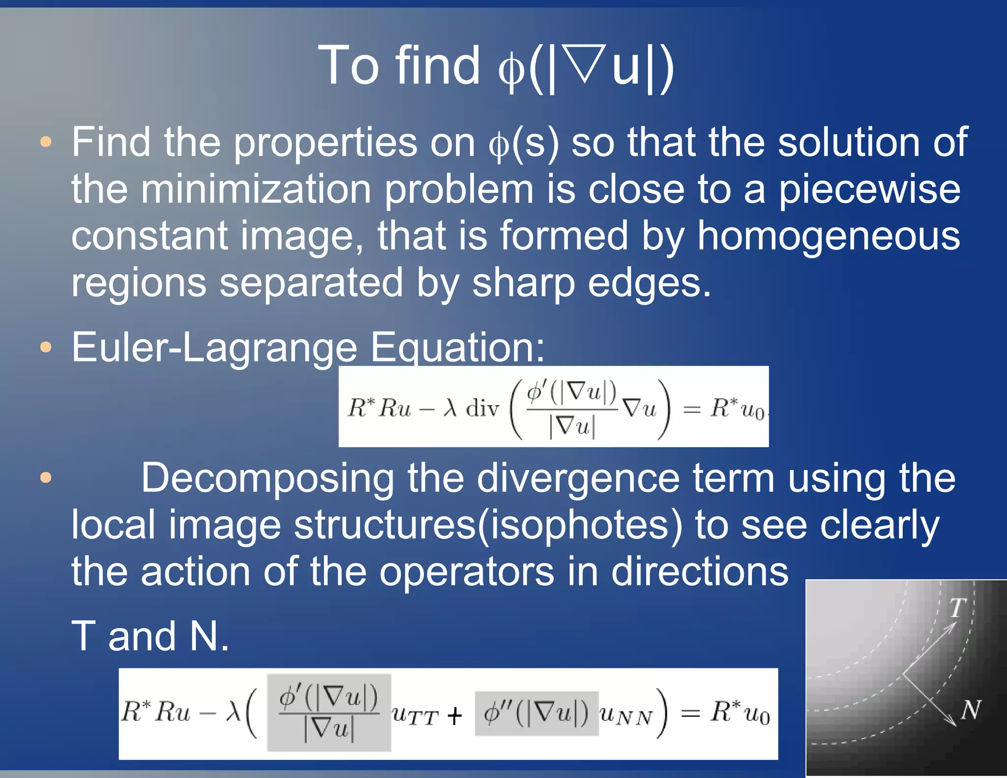
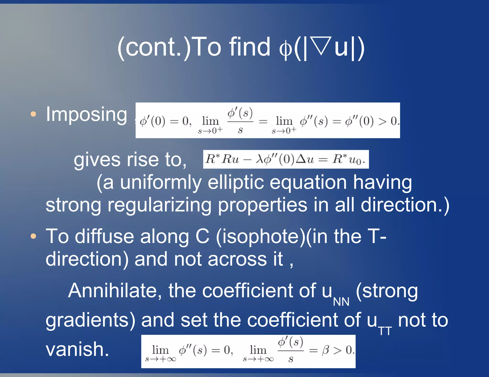
Total Variation (L1
-▽) Minimization
● As Laplacian Operator has very strong
isotropic smoothing properties , edges are not
preserved.
●
The Lp
norm with p = 2 of the gradient allows to
remove the noise but penalizes much of the
gradients(edges).
● [Rudin, Osher and Fatemi]: Decrease p in order to
keep as much as possible the edges.

To find ϕ(|▽u|)
● Find the properties on ϕ(s) so that the solution of
the minimization problem is close to a piecewise
constant image, that is formed by homogeneous
regions separated by sharp edges.
● Euler-Lagrange Equation:
● Decomposing the divergence term using the
local image structures(isophotes) to see clearly
the action of the operators in directions
T and N.

(cont.)To find ϕ(|▽u|)
● Imposing ,
gives rise to,
(a uniformly elliptic equation having
strong regularizing properties in all direction.)
● To diffuse along C (isophote)(in the T-
direction) and not across it ,
Annihilate, the coefficient of uNN
(strong
gradients) and set the coefficient of uTT
not to
vanish.

Performance Metrics[wang, et. al]
● Figure of Merit Metric (FOM): (Edge
preserving measure)
where N^ and Nideal
are the total numbers of detected and original edge pixels,
respectively;
● di
is the Euclidean distance between the ith
detected edge pixel and
the nearest original edge pixel;
● λ is a constant typically set to 1/9.
● The dynamic range of FOM is between the processed image and the
ideal image.

● Structural Similarity Metric(SSIM):
Let x={xi
}; y={yi
} be the original and the test
images.
This quality index models any distortion as
a combination of 3 different factors:
loss of correlation,
luminance distortion, and
contrast distortion.
● The dynamic range of SIMM is [-1,1]

● Mean Square Error Metric (MSE):
The smaller the MSE value, the better is the
denoising performance.
● SNR Metric:
when the denoised image has a large
SNR it will be closer to the original image and
will have a better quality.

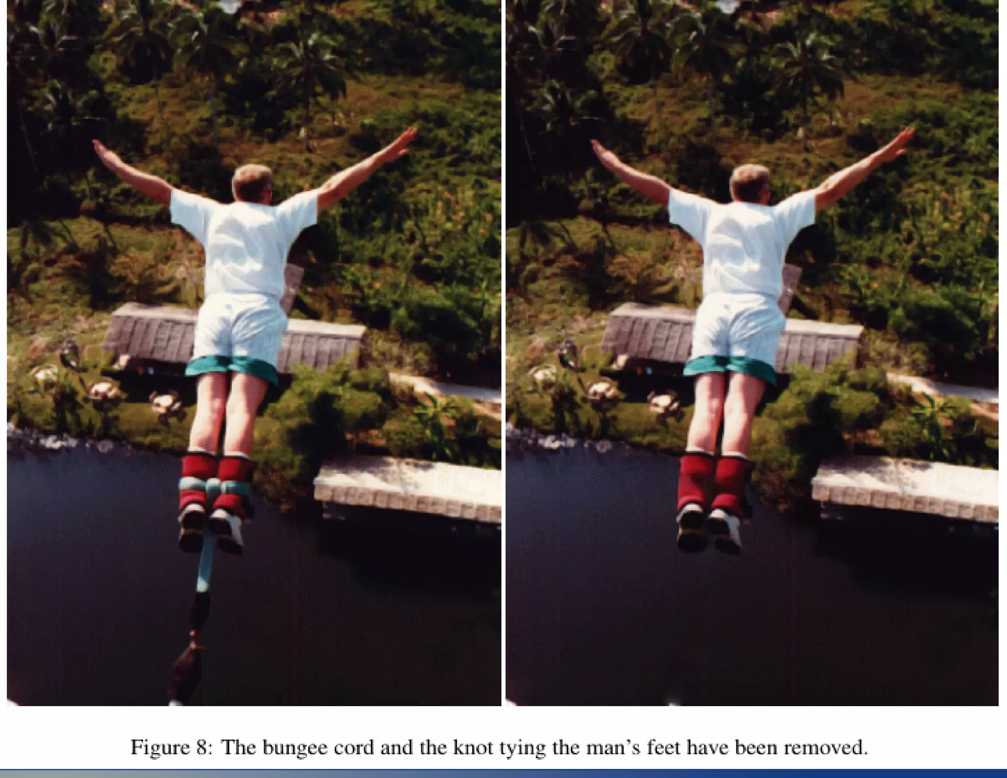
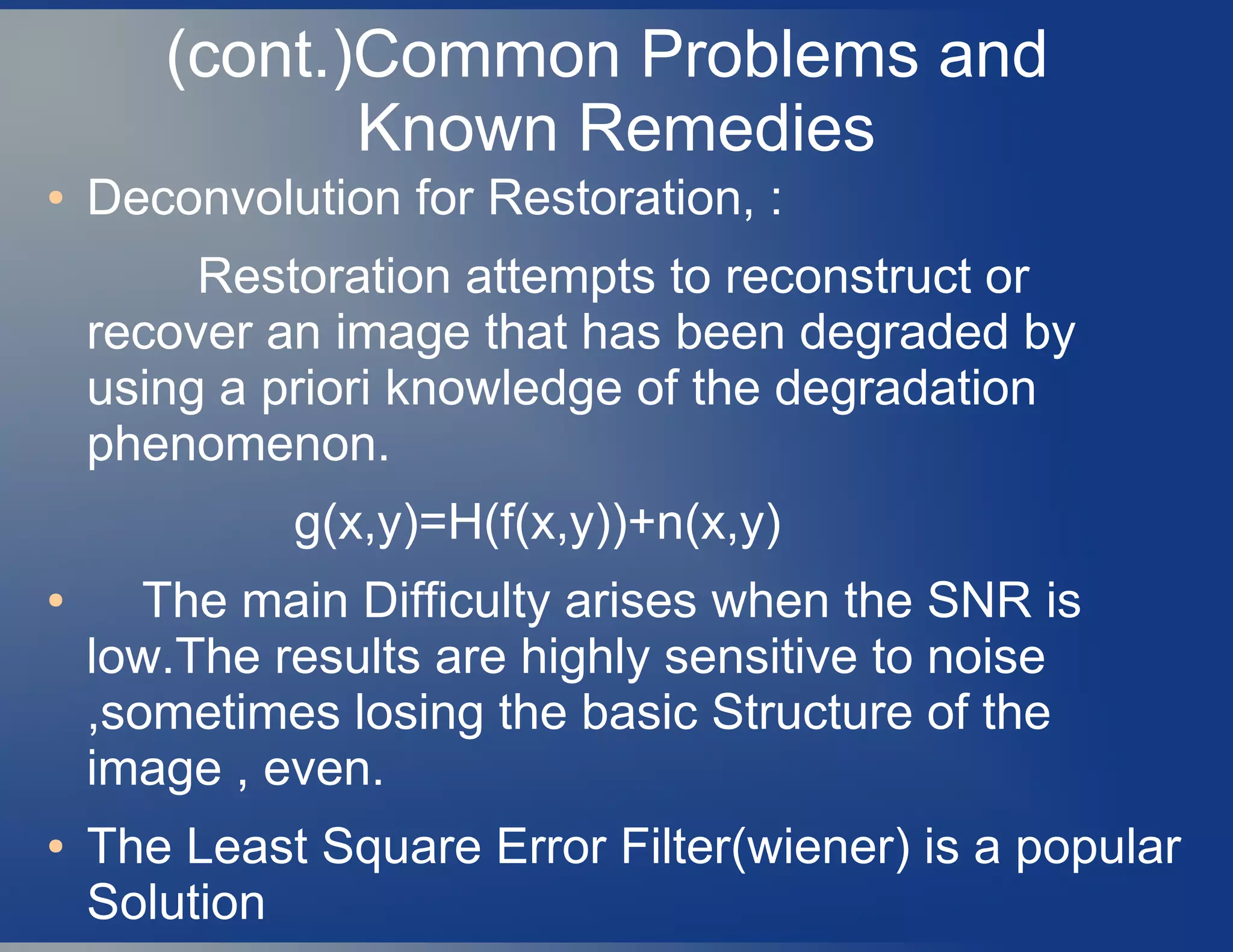
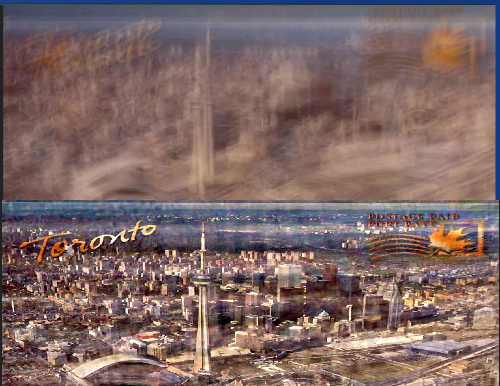
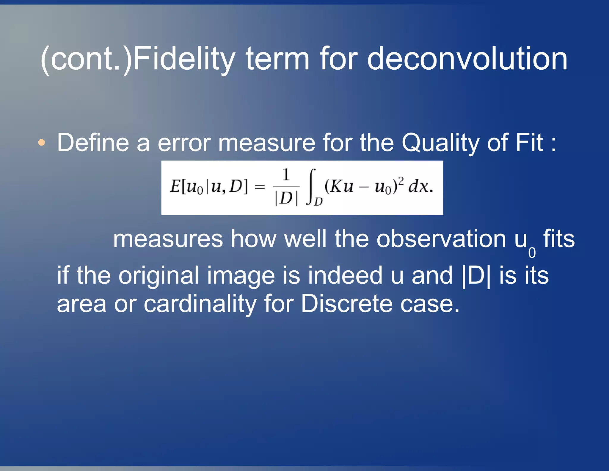
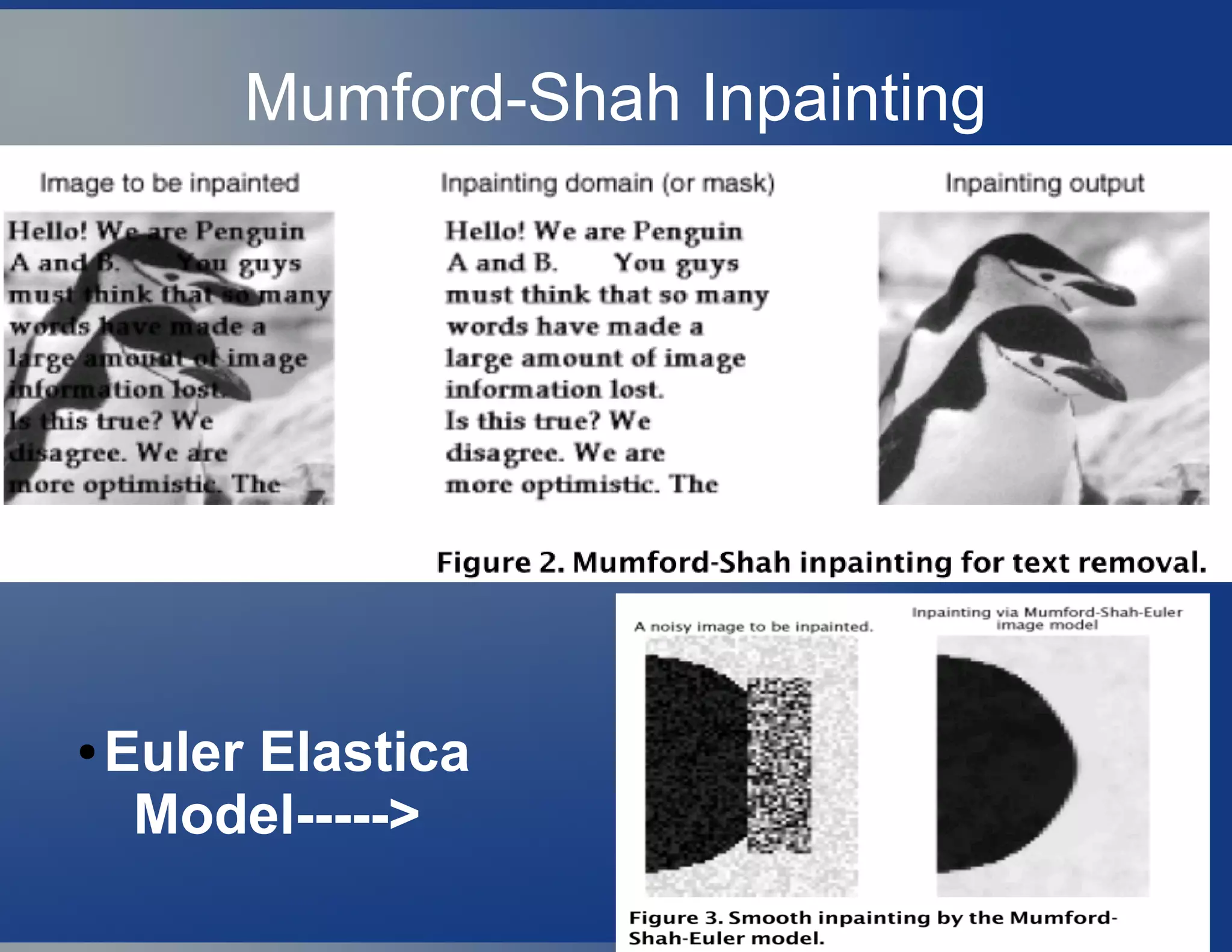
Image Inpainting
● u0
denotes the observed(noisy or blurry) portion
of u, on a sub domain D. The goal of inpainting
is to recover u on the entire image domain Ω.
● A simple Geometric Model is , with blurring
followed by noise degradation and spatial
restriction.
where K is a continuous blurring kernel
(linear,shift-invariant), and η is an additive
white noise field assumed to be close to
Gaussian for simplicity &the information [u0
]ΩD
is missing.

(cont.)Fidelity term for deconvolution
● Define a error measure for the Quality of Fit :
measures how well the observation u0
fits
if the original image is indeed u and |D| is its
area or cardinality for Discrete case.

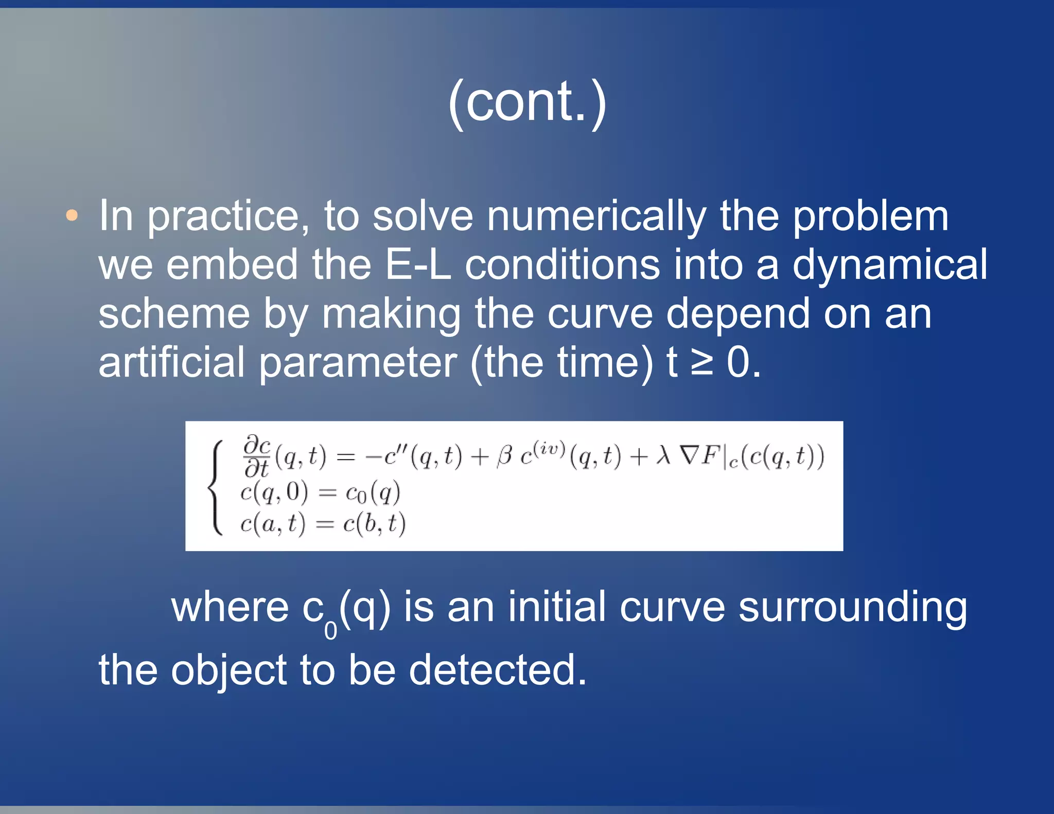
(cont.)Regularity Condition E[u]
● Regularity of the new Image(u) is enforced
through The “energy” functionals: { E[u] }
● Then the Image Inpainting becomes a
constrained optimization problem:
min E[u] over all u such that E[u0
|u] ≤ σ2
Here σ2
(variance of the white noise), is
assumed to be known by proper statistical
estimators.

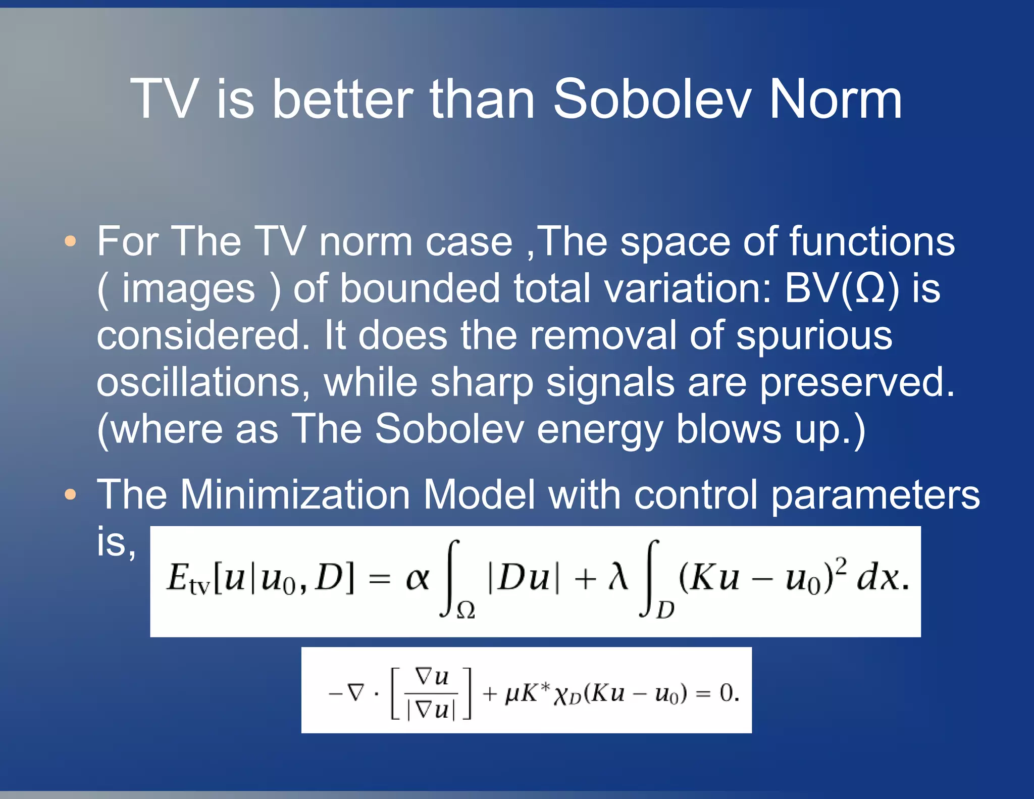
Examples of E[u]
● Sobolev norm E[u] =∫Ω
| u|∇ 2
dx,
● The total variation (TV) model E[u] =∫Ω
|Du| of
Rudin, Osher, and Fatemi, and
● The Mumford-Shah free-boundary model
E[u,Γ] =∫ΩΓ
| u|∇ 2
dx + βH1
(Γ),
where H1
denotes the one-dimensional
Hausdorff measure.

TV is better than Sobolev Norm
● For The TV norm case ,The space of functions
( images ) of bounded total variation: BV(Ω) is
considered. It does the removal of spurious
oscillations, while sharp signals are preserved.
(where as The Sobolev energy blows up.)
● The Minimization Model with control parameters
is,

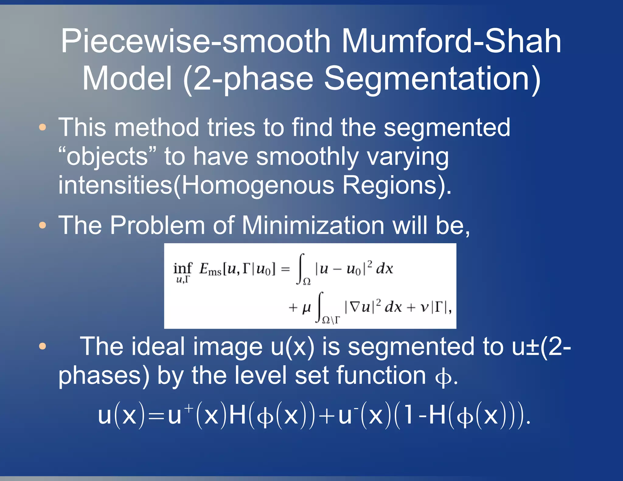
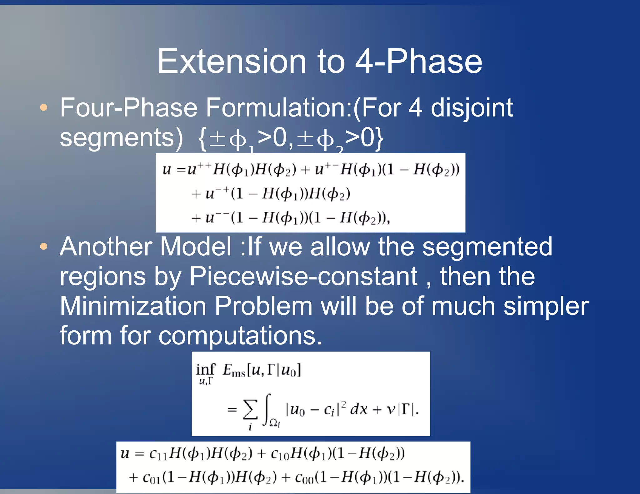
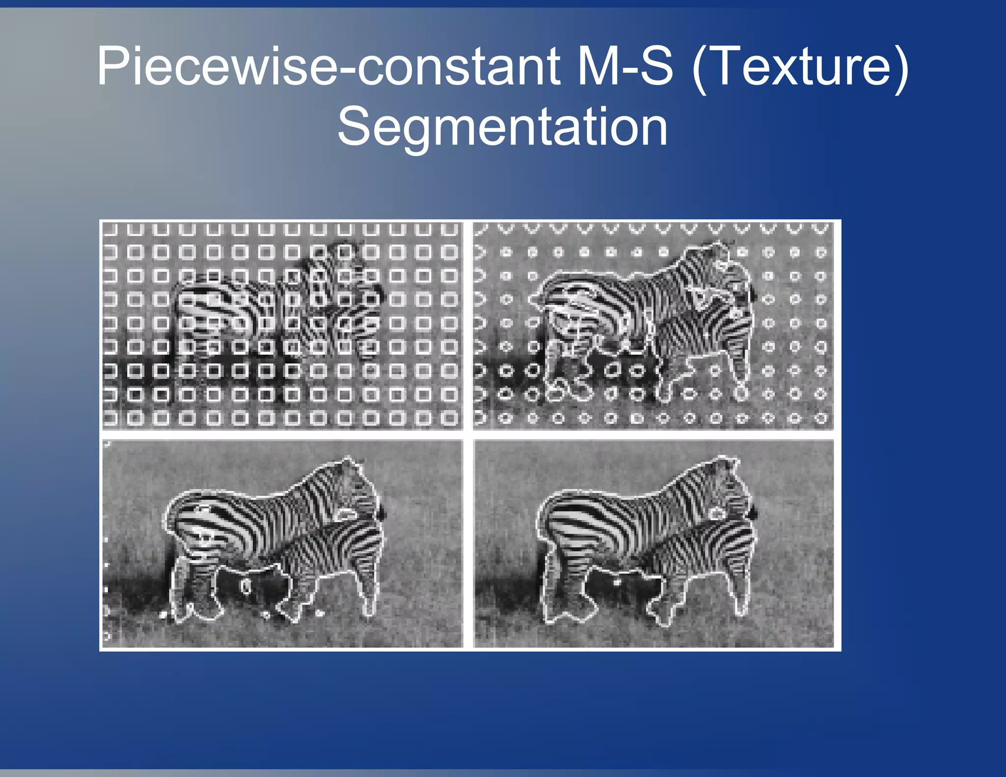
The object-edge model [Ems
]
[Mumford and Shah]
● An image u is understood as a combination of
both the geometric feature Γ and the
piecewise smooth “objects” ui
on all the
connected components Ωi
of Ω Γ , assuming
Γ to be Lipschitz. And the smoothness of the
“objects” characterized by Sobolev Norm.

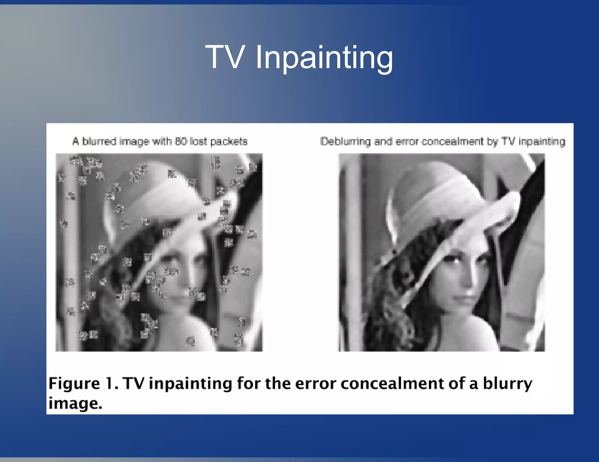
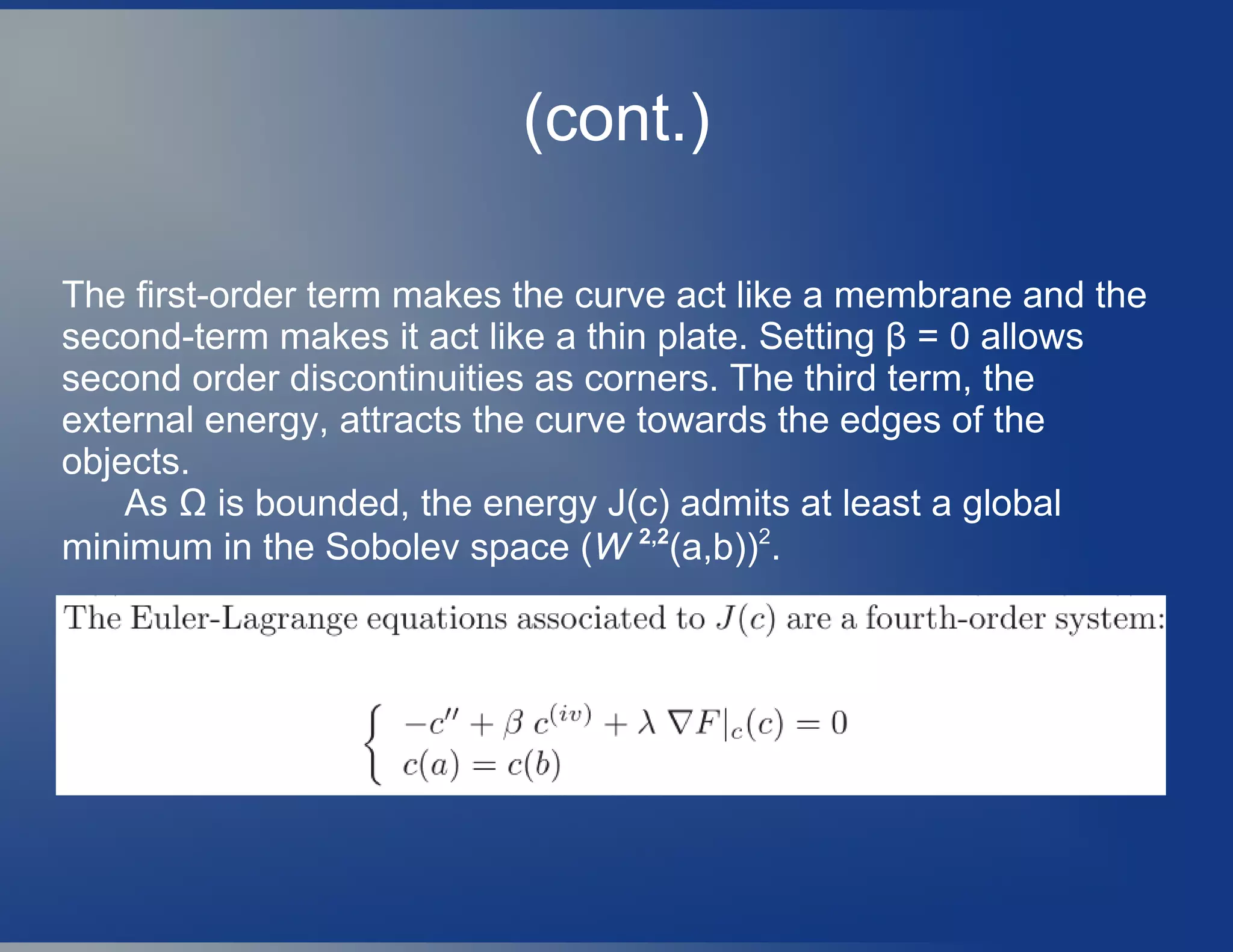
(cont.)Higher-order geometric
Image Models
● [Esedoglu and Shen]: For large-scale
inpainting problems, high-order image models
which incorporate the curvature information
become necessary for more faithful visual
effects.
Replacing length energy by Euler's
elastica Energy:
● The curvature is given by

● Euler Elastica
Model----->
Mumford-Shah Inpainting

Image Segmentation
● Images are the proper 2-D projections of the 3-D world
containing various objects.
● Segmentation is to identify the regions in images that
correspond to individual objects.
● Denote by u0
an observed image on a 2-D Lipschitz
open and bounded domain Ω.
● Segmentation means finding a visually meaningful
edge set Γ that leads to a complete partition of Ω.
Each connected component Ωi
of ΩΓ should
correspond to at most one real physical object or
pattern in our 3-D world, for example, the white matter
in brain images.

Piecewise-smooth Mumford-Shah
Model (2-phase Segmentation)
● This method tries to find the segmented
“objects” to have smoothly varying
intensities(Homogenous Regions).
● The Problem of Minimization will be,
● The ideal image u(x) is segmented to u±(2-
phases) by the level set function .
( )=u x u+
( ) (x H ( ))+x u-
( )( - (x 1 H ( ))).x

(First Stage) Denoising the regions
●
Assuming, both u+ and u- are C1
functions up
to the boundary { = 0} ,Minimize the Energy ,
● First, with  fixed, the variation on E[u+,u-,|
u0
] leads to the two Euler-Lagrange equations
for u± separately. These act as denoising
operators on the homogeneous regions
only,not on edge set{=0}

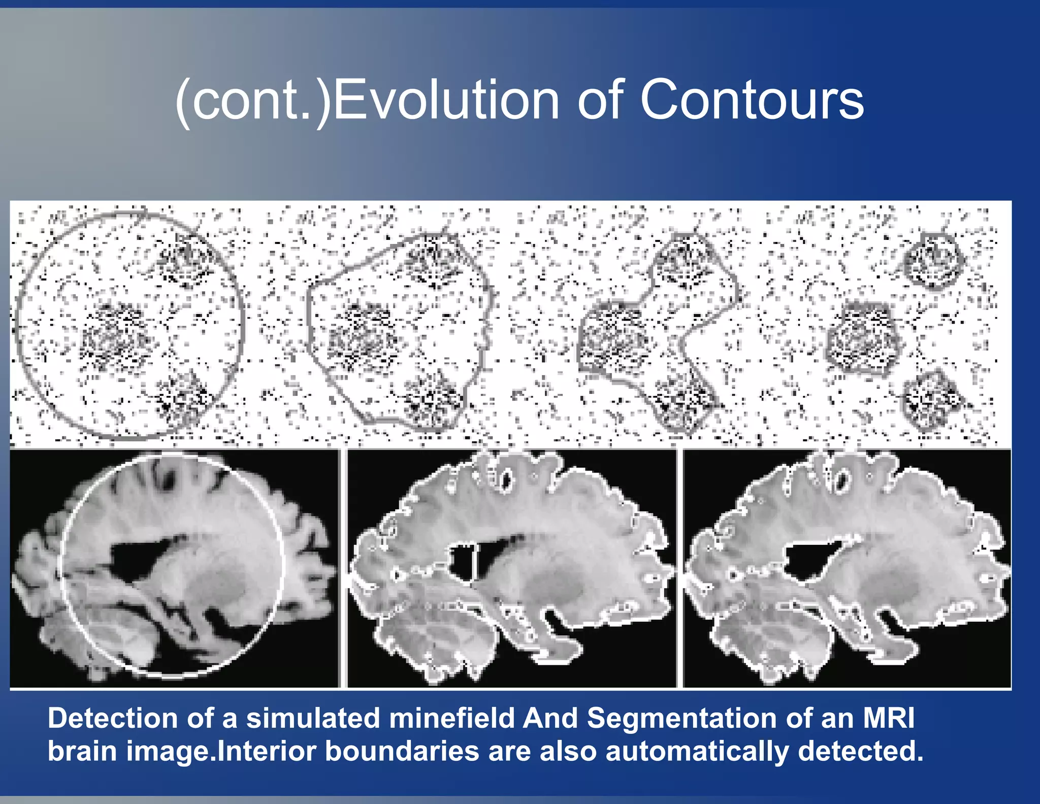
(Second stage)Contour evolution
● Next, keeping the functions u+ and u- fixed
and minimizing E[u+,u-,|u0] with respect to
, we obtain the motion of the zero-level set
with some initial guess (t=0,x).
This single model, which includes both the
original energy formulation And the elliptic and
evolutionary PDEs ,naturally combining all
three image processors —active contour,
segmentation, and denoising.

(cont.)Evolution of contours &
region smoothing

Extension to 4-Phase
● Four-Phase Formulation:(For 4 disjoint
segments) {1
>0,2
>0}
● Another Model :If we allow the segmented
regions by Piecewise-constant , then the
Minimization Problem will be of much simpler
form for computations.

Piecewise-constant M-S (Texture)
Segmentation

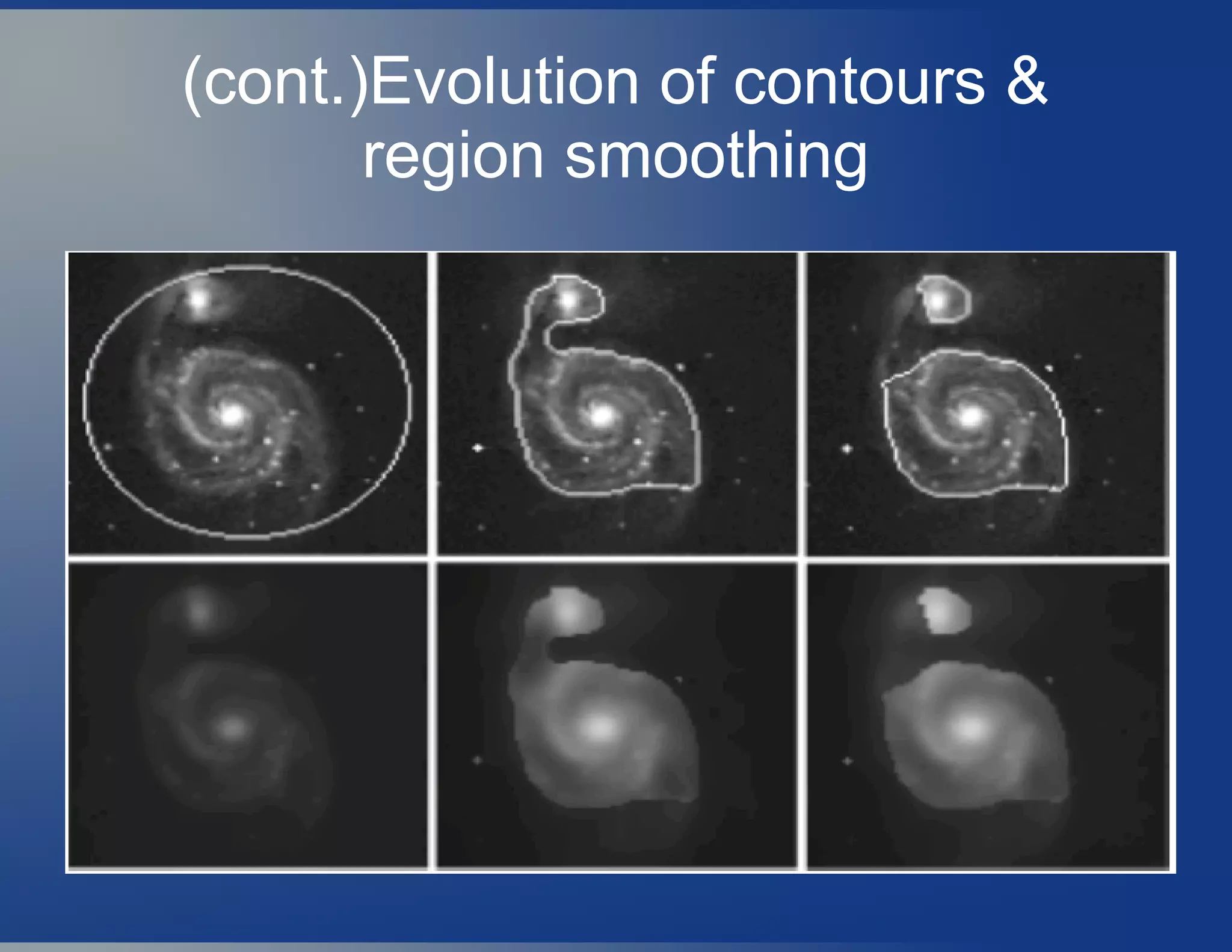
Active contours without Edges(snakes)
[The Kass-Witkin-Terzopoulos]
Unlike the Mumford and Shah functional, the aim is
no longer to find a partition of the image but to
automatically detect contours of objects,starting from a
initial guess and g(s),an Edge-detector function.
Working: Boundary detection consists in matching a
deformable model to an image by means of energy
minimization.

Detection of a simulated minefield And Segmentation of an MRI
brain image.Interior boundaries are also automatically detected.
(cont.)Evolution of Contours

(cont.)
The first-order term makes the curve act like a membrane and the
second-term makes it act like a thin plate. Setting β = 0 allows
second order discontinuities as corners. The third term, the
external energy, attracts the curve towards the edges of the
objects.
As Ω is bounded, the energy J(c) admits at least a global
minimum in the Sobolev space (W 2,2
(a,b))2
.

(cont.)
● In practice, to solve numerically the problem
we embed the E-L conditions into a dynamical
scheme by making the curve depend on an
artificial parameter (the time) t ≥ 0.
where c0
(q) is an initial curve surrounding
the object to be detected.

Neurons & Signal Transmission
Neurons receive information either at
their dendrites or cell bodies. The axon
of a nerve cell is, in general,
responsible for transmitting information
over a relatively long distance.
Therefore, most neural pathways are
made up of axons. If the axons have
myelin sheaths, then the pathway
appears bright white because myelin is
primarily lipid. If most or all of the
axons lack myelin sheaths , then the
pathway will appear a darker beige
color, which is generally called gray,

What is Tractography?
● A neural pathway(tract),
connects one part of the
nervous system with
another and usually
consists of bundles of
elongated, myelin-
insulated neurons, known
collectively as white
matter.
● Neural pathways serve to
connect relatively distant
areas of the brain or
nervous system, compared
to the local communication
of grey matter.

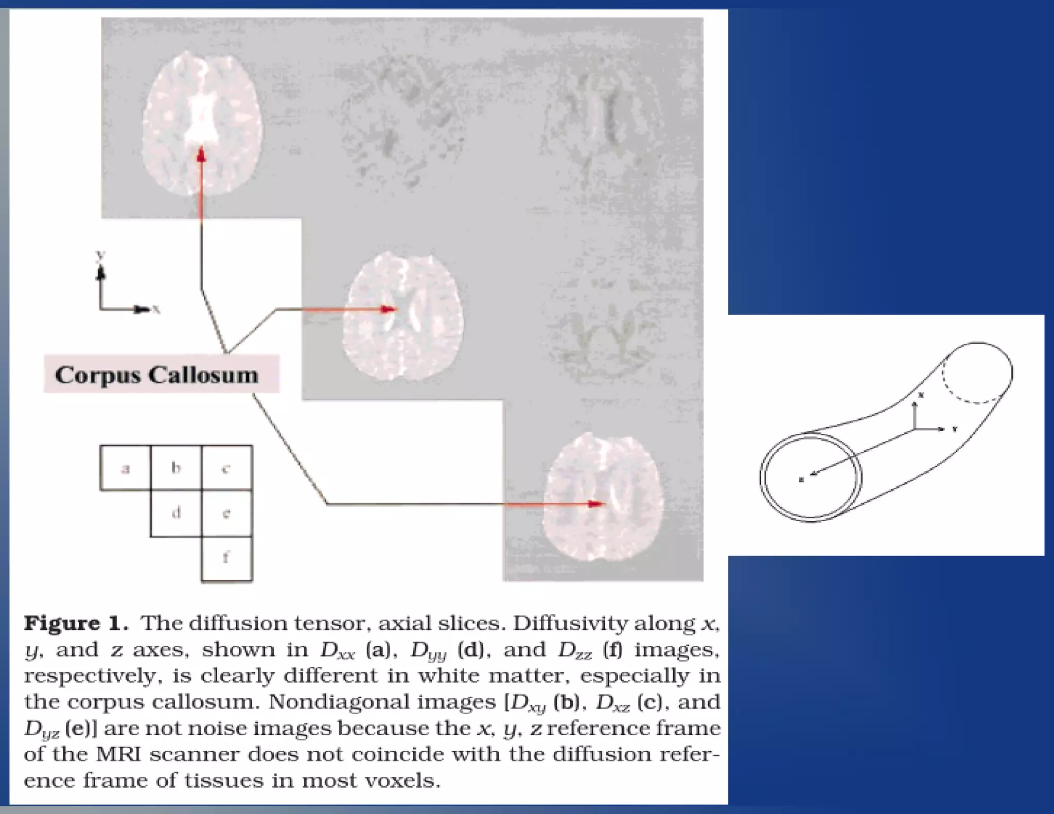
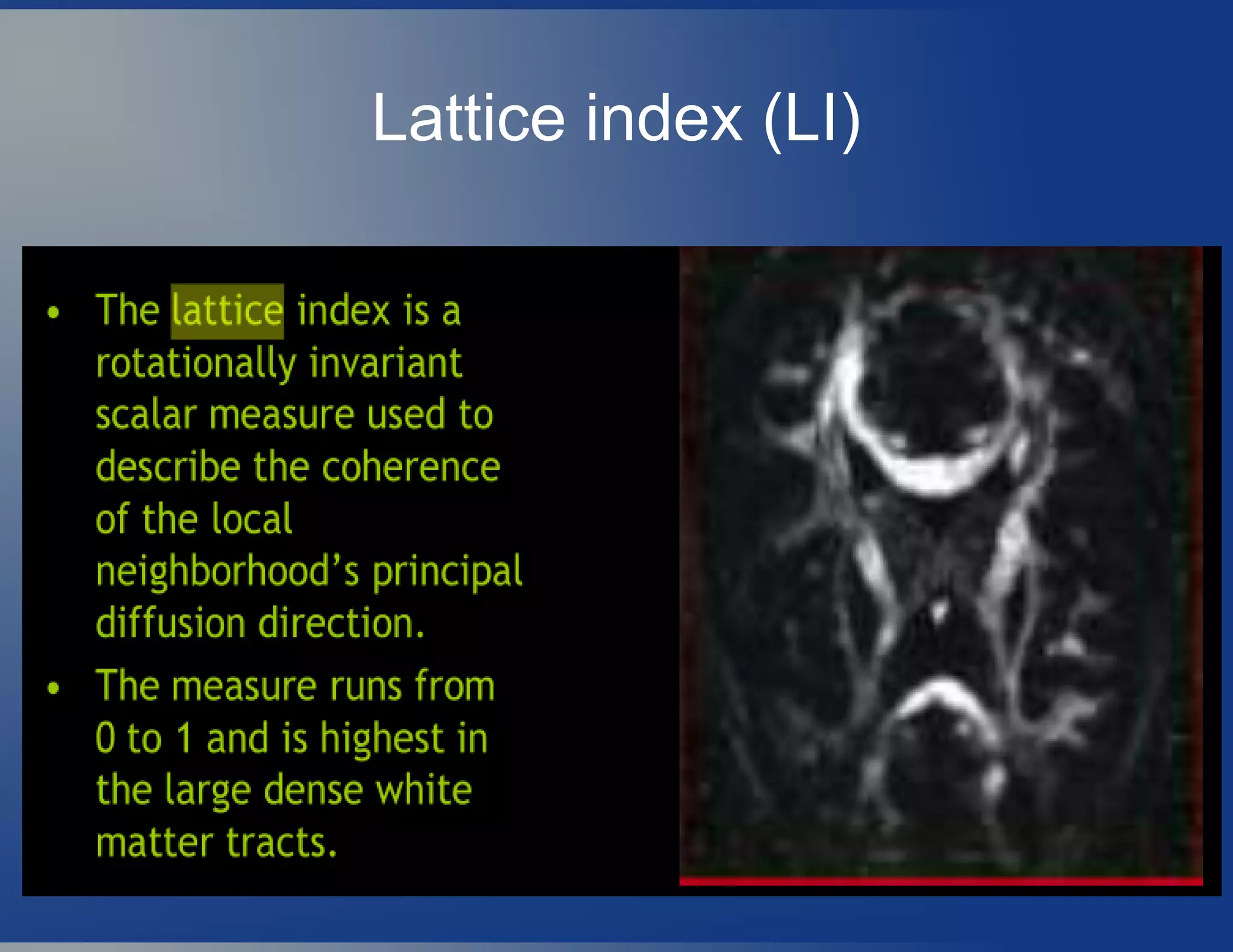
DT-MRI[Denis Le Bihan]
● THE BASIC PRINCIPLES of diffusion MRI were
introduced in the mid-1980s [Taylor et al,1985]; they
combined NMR imaging principles with those
introduced earlier to encode molecular diffusion
effects in the NMR signal by using bipolar magnetic
field gradient pulses .
● Molecular diffusion refers to the random translational
motion of molecules, also called Brownian motion, that
results from the thermal energy carried by these
molecules.
● These random, diffusion driven displacements
molecules probe tissue structure at a microscopic
scale well beyond the usual image resolution:

Diffusion tensor
‖Dan
Measures the deviation of diffusion Tensor‖
from Isotropy

Geometrical Measures of Diffusion

Existing Approaches for Fibre
Tracking
● Using principle eigen direction.
● Navier stokes-GGVF-Active contours(snakes)
● Using Heat Diffusion Equation-GGVF-Snakes

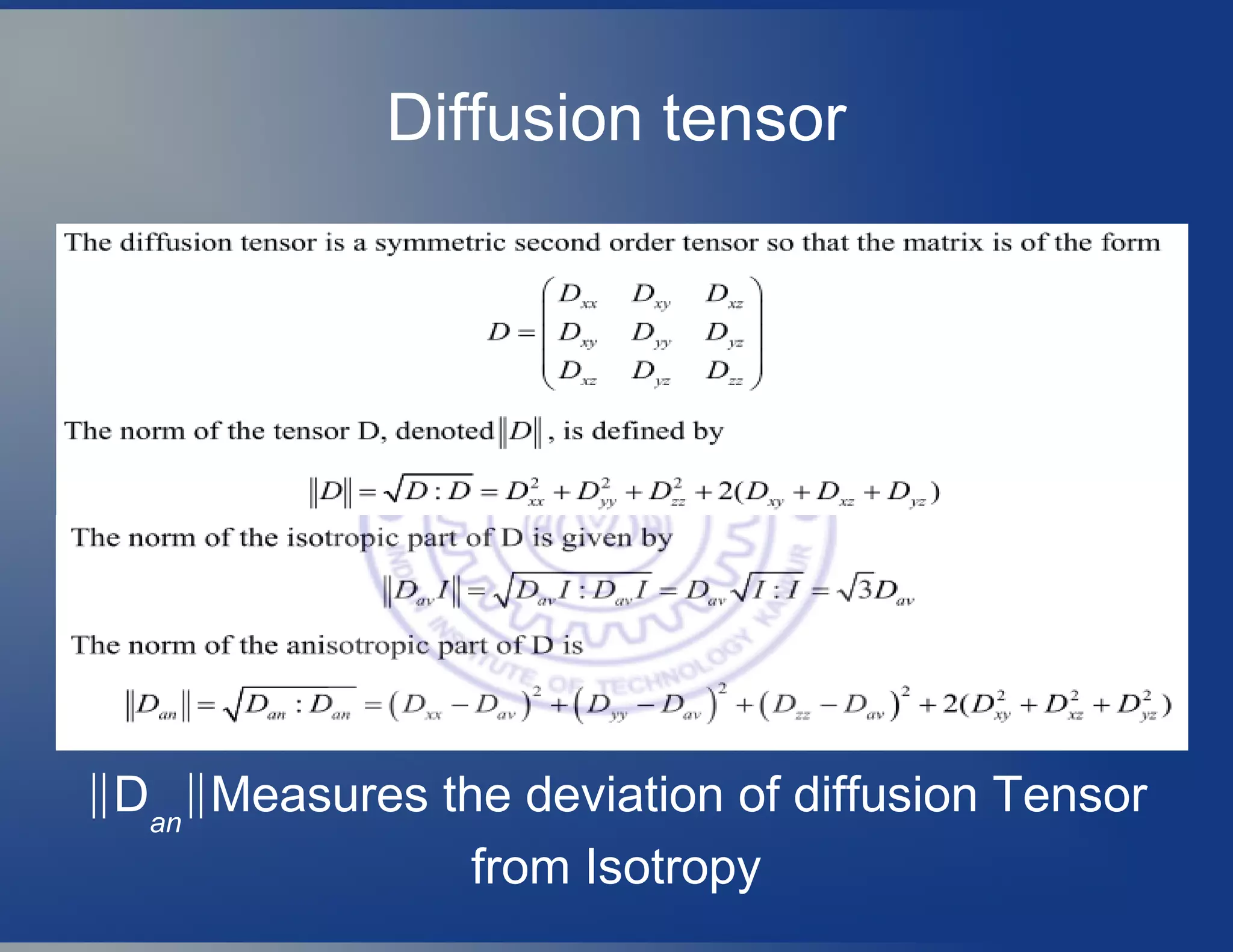
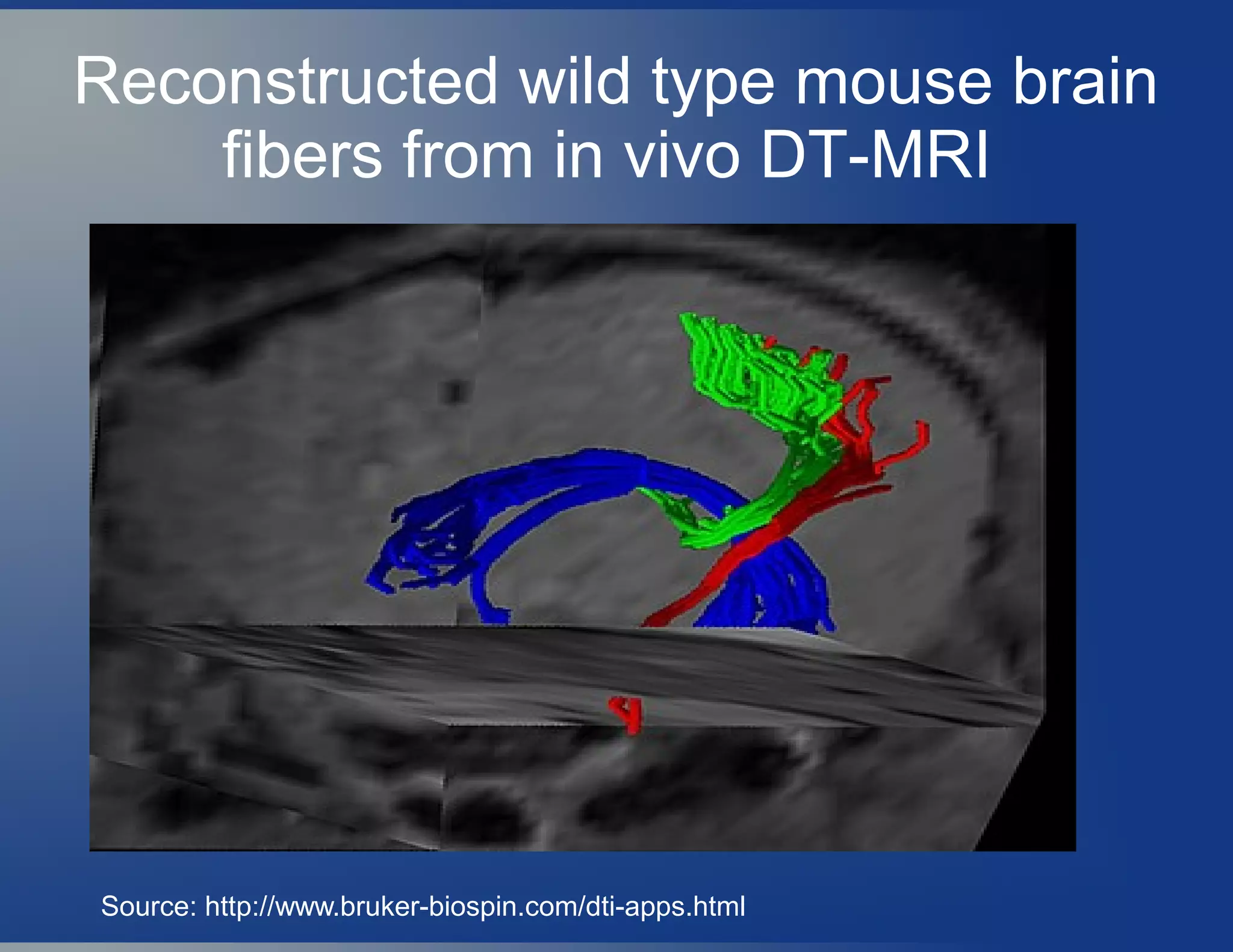
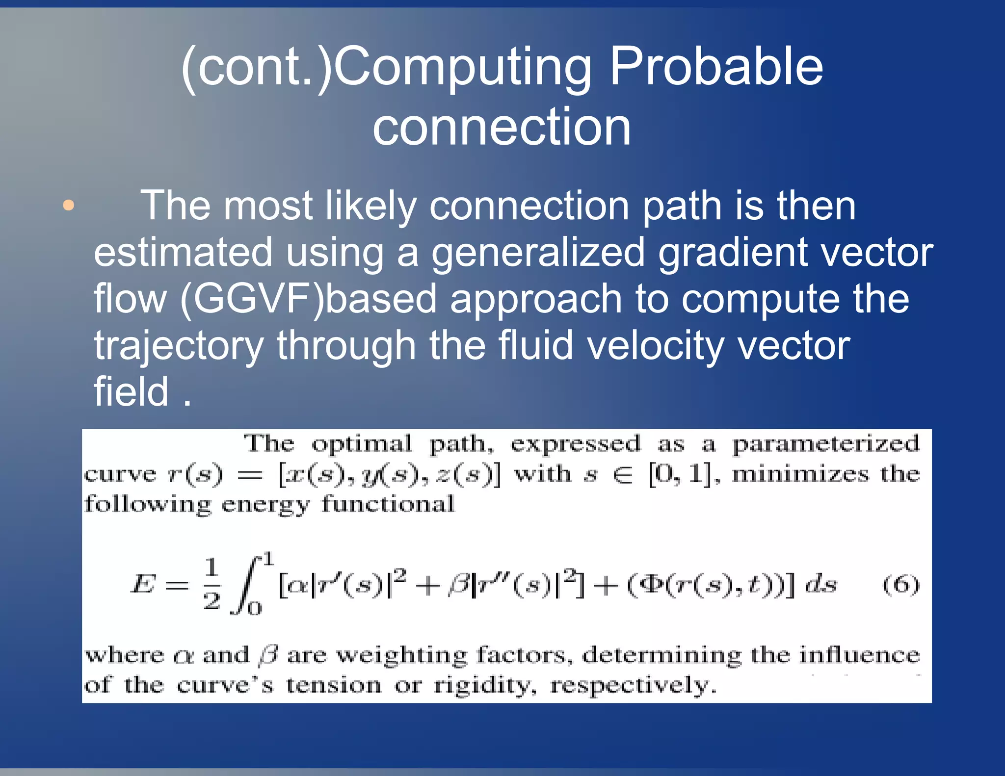
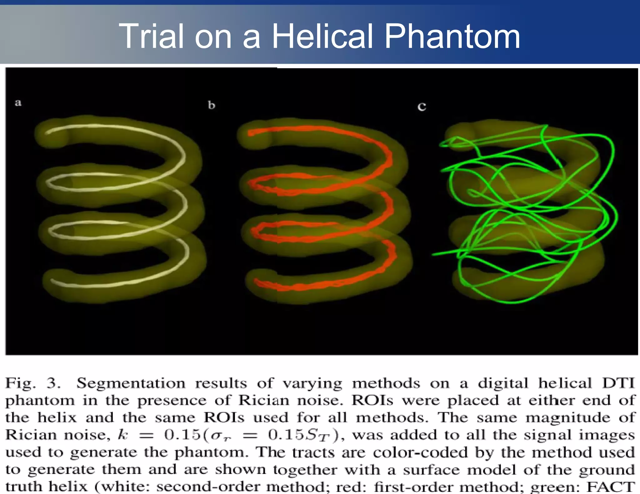
Fibre Assignment by Continuous
Tracking(FACT)
● Each Voxel at postion (x,y,z) is characterized
by Second order diffusion Tensor D which
represents the local 3D anisotropic Gaussian
diffusion process
● To infer continuity of Fibre orientation from
voxel to voxel and to reconstruct the
connections between the brain regions
[Basser et al,2000] , a 3D-arc length
parametrized trajectory r(s) ,has been
proposed as , and is solved
for r(s) ,starting from a seed
position r0
=r(s0
).

Reconstructed wild type mouse brain
fibers from in vivo DT-MRI
Source: http://www.bruker-biospin.com/dti-apps.html

Using Navier Stokes equations
● simulate the flow of an artificial fluid governed
by the Navier–Stokes equations.
● Using Finite volume method to approximate
the solution ,solution of the steady state is
found by,

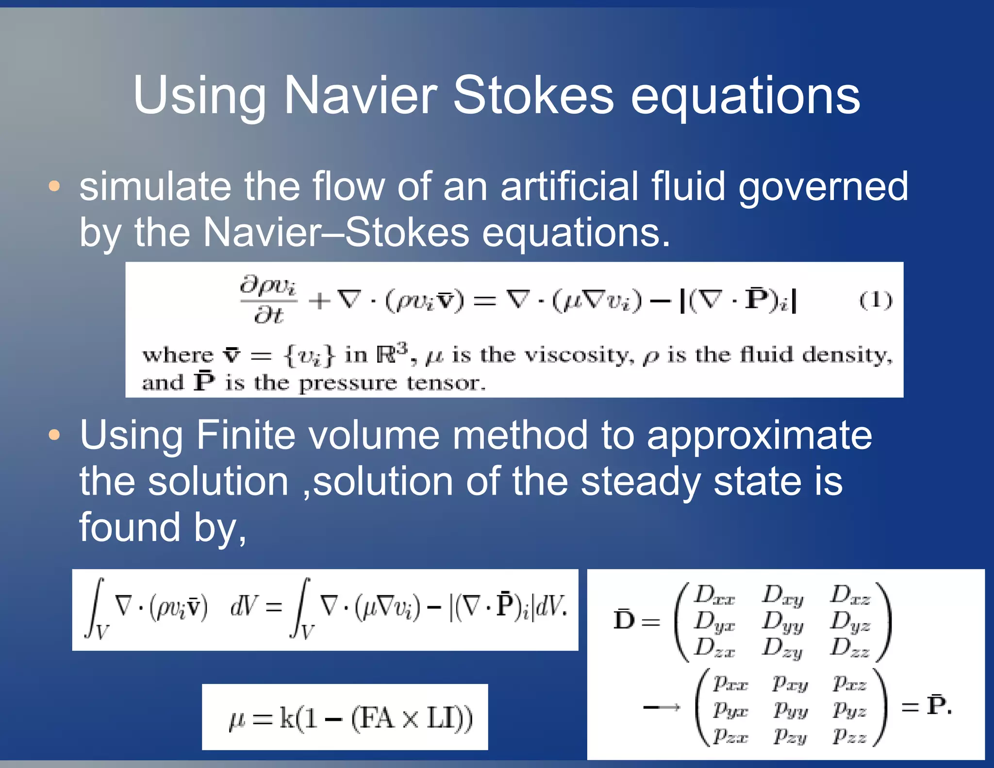
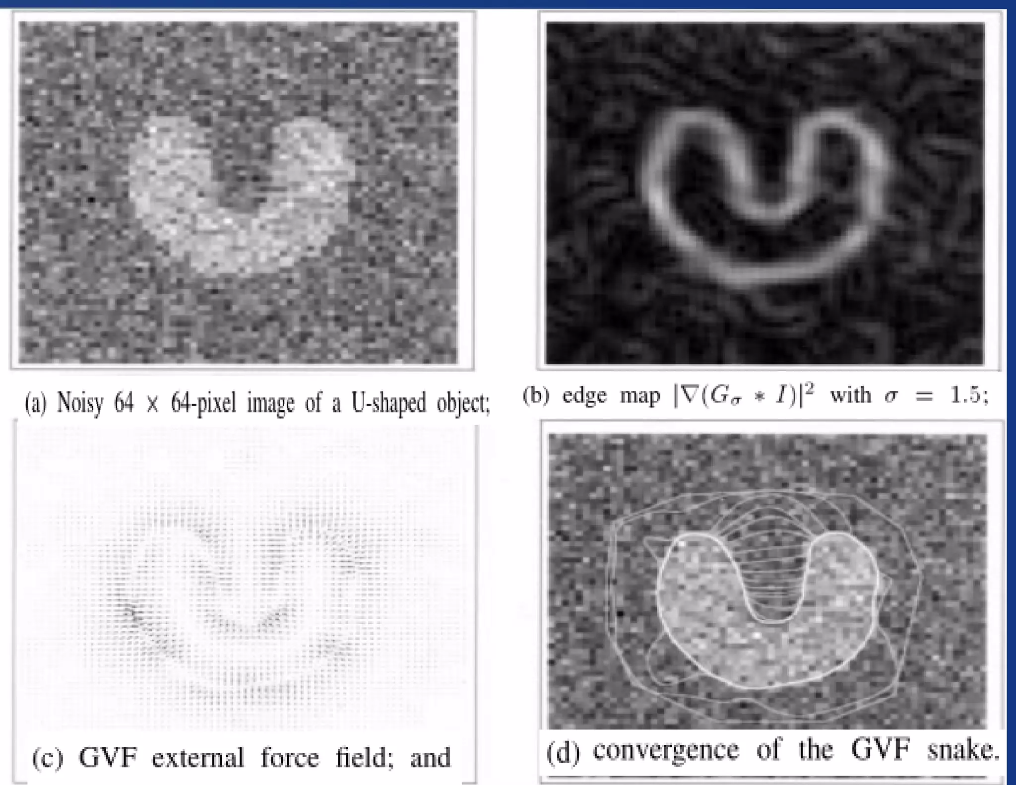
Gradient Vector Flow(GVF)
(new external force for Snakes )
● [Xu et. al,1998]-Define the gradient vector flow
field to be the vector field Φ(x,y)=[u(x,y),v(x,y)]
that minimizes the energy functional ,
where f is the fluid volume & when |▽f| is
large, the 2nd
term dominates the integrand, and
is minimized by setting Φ=▽ ,f producing the
desired effect of keeping Φ(x,y) nearly equal to
the gradient of the edge map and also forcing
the field to be slowly-varying in homogeneous
regions.

(cont.)
● Solve the E-L Equations , for Φ(x,y) that
minimizes The Energy functional ,

(cont.)Computing Probable
connection
● The most likely connection path is then
estimated using a generalized gradient vector
flow (GGVF)based approach to compute the
trajectory through the fluid velocity vector
field .

Tract connecting the ROI's using
GGVF instead of GVF

Heat Diffusion Equation based
Tractography
● Generate The Heat flow vector Field , using :

Metric of Tract Fidelity
(to compare the methods)
Average fractional
Anisotropy:
The principal eigen
vector, defines the main
direction of diffusion of water
molecules in that voxel.
Chose a path that gives
Maximum of the integral of
innerproduct (path and
principal direction) multiplied
by FA.
Maximum Inner product
colour coded Map:

On HARDI data
● DT-MRI implicitly assumes that the diffusion is
Gaussian everywhere when estimating intra-
voxel diffusion configurations where more than
one single fiber direction predominates.
● DTI cannot model crossing or kissing fibers
but it also estimates wrong directions in the
case of multiple fiber configurations
● High Angular Resolution Diffusion Imaging
(HARDI) comes as an interesting alternative
as it samples the diffusion signal only on the
single sphere following discrete gradient
directions;.

Proposed work
● To take advantage of adaptive grids in computations
from Finite element methods.
● To work on 3D-Image data (stacks) with the
knowledge from Differential Geometry.
● Applications to Brain tractography segmentation for
HARDI.
● To Frame, segmentation problems using cahn-hilliard
equation (reverse diffusion) for binary fluids.
● Enhancing the performance of ill-posed problems by
suitable addition of arguments.
●
Test various models with the Norm of L1+ϵ

Cahn-hilliard Evolution of random
initial data γ=0.5 and C=0,
demonstrating phase separation

Sources
● A. Witkin. “Scale-space filtering." Int. Joint Conf. Artificiul
Inrelligence, Karlsiuhe. West Germany. 1983. pp. 1019-1021
● J. Koenderink. "The structure of images." Biol. Cybern. vol. 50.pp.
363-370, 1984.
● P. PERONA and J. MALIK, Scale space and edge detection using
anisotropic diffusion, Proc. IEEE Computer Soc. Workshop on
Computer Vision, 1987.
● Y. You and M. Kaveh, Fourth order partial differential equations for
noise removal, IEEE Trans. Image Processing, vol. 9, no. 10, 2000,
pp 1723-1730.
● M. Lysaker, A. Lundervold and X. Tai, Noise removal using fourth
order partial differential equation with applications to medical
magnetic resonance images in space and time, IEEE Trans. Image
Processing, vol. 12, no. 12, 2003,pp 1579 – 1590.

Sources
● R. T. Whitaker and S. M. Pizer, “A multi-scale approach to
nonuniform diffusion,” Comput. Vis. Graph. Image Process.: Image
Understand., vol. 57, pp. 99–110, Jan. 1993.
● L. Alvarez, F. Guichard, P.L. Lions, and J.M. Morel. Axioms and
fundamental equations of image processing. Archive for Rational
Mechanics and Analysis, 123(3):199–257, 1993.
● J. Canny, “A computational approach to edge detection,” IEEE
Trans. Pattern Anal. Machine Intell., vol. PAMI-8, pp. 679-698, 1986.
● Z.Wang and A.C. Bovik, A Universal Image quality index, IEEE Signal
Processing letters, vo.9,no.3,pp-81-84,2002.
● T.F. Chan, J. Shen and L. Vese, Variational PDE Models in Image
Processing, December 2002.

sources
● Bazan, C, Blomgren,Adaptive Finite Element Method for Image
Processing Solution after 2 iterations using adaptive mesh
,Proceedings of the COMSOL Multiphysics User's Conference 2005
Boston
● Hamidreza K,Nadernejad, E ;PDEs-Based Method for Image
Enhancement ,Applied Mathematical Sciences, Vol. 2, 2008, no. 20,
981 - 993
● Nadernejad, E, Sharifzadeh, Sara ; Hassanpour, Hamid ,Edge
Detection Techniques: Evaluations and Comparison ,Applied
Mathematical Sciences , vol: 2, issue: 31, pages: 1507-1520, 2008.
● Taylor DG, Bushell MC. The spatial mapping of translational
diffusion coefficients by the NMR imaging technique. Phys Med
Biol,1985;30:345–349.
● S. Esedoglu and J. Shen. Digital inpainting based on the Mumford-
Shah-Euler image model. European J. Appl. Math., in press, 2002.

sources
● H.-K. Zhao, T. F. Chan, B. Merriman, and S. Osher. A
variational level set approach to multiphase motion. J.
Comput. Phys., 127, 179-195
● Denis Le Bihan,Jean-Francois Mangin,Cyril Poupon,Chris
A. Clark, Sabina Pappata,Nicolas Molko,Hughes
Chabriat,Diffusion Tensor Imaging: Concepts and
Applications ,JOURNAL OF MAGNETIC RESONANCE
IMAGING 13:534–546 (2001).
● P. Basser, J. Mattiello, and D. Le Bihan, “Estimation of the
effective self-diffusion tensor from the NMR spin echo,” J.
Magn. Reson., vol.103, pp. 247–254, 1994.
● Rathore R.K.S.,Geetaneh Bayu,Ankur P,Shruthi A, Fibre
Tracking and visualization in DT-MRI ,PhD Thesis IIT
Kanpur ,2008.

sources
● N. Kang, J. Zhang, E. S. Carlson, and D. Gembris, “White matter fiber
tractography via anisotropic diffusion simulation in the human
brain,”IEEE Trans. Med. Imag., vol. 24, no. 9, pp. 1127–1137, Sep.
2005
● Nathan S. Hageman,Arthur W. Toga,Katherine L. Narr,A Diffusion
Tensor Imaging Tractography Algorithm Based on Navier–Stokes
Fluid Mechanics;IEEE TRANSACTIONS ON MEDICAL IMAGING,
VOL. 28, NO. 3, MARCH 2009.
● Daniel S. Reich, Arzu Ozturk, Peter A. Calabresi, Susumu
Mori,Automated vs. conventional tractography in multiple sclerosis:
Variability and correlation with disability Original Research Article
NeuroImage, Volume 49, Issue 4, 15 February 2010, Pages 3047-
3056 .
● White matter atlas generation using HARDI based automated
parcellation Original Research Article NeuroImage, Volume 59, Issue
4, 15 February 2012, Pages 4055-4063 Luke Bloy, Madhura
Ingalhalikar, Harini Eavani, Robert T. Schultz, Timothy P.L. Roberts,
Ragini Verma

State of art pde based ip to bt vijayakrishna rowthu

Recommended

Recommended

More Related Content

What's hot

What's hot (18)

Similar to State of art pde based ip to bt vijayakrishna rowthu

Similar to State of art pde based ip to bt vijayakrishna rowthu (20)

Recently uploaded

Recently uploaded (20)

State of art pde based ip to bt vijayakrishna rowthu