Drive Engineering – Practical Implementation
1052 2913 / EN
Project Planning of Drives
Edition
10/2001
SEW-EURODRIVE GmbH & Co · P.O.Box 3023 · D-76642 Bruchsal/Germany · Phone +49-7251-75-0
Fax +49-72 51-75-1970 · http://www.SEW-EURODRIVE.com · sew@sew-eurodrive.com
Geared Motors  Drive Electronics  Drive Automation  ServicesGeared Motors  Drive Electronics  Drive Automation  Services
Contents
1
2
3
4
5
6
7
8
9
10
11
12
13
14
15
16
17
18
Drive Engineering – Practical Implementation – Project Planning of Drives 3
1 Introduction ....................................................................................................... 6
2 AC drives with fixed speeds ............................................................................ 9
3 AC drives with frequency inverter................................................................. 26
4 Servo drives..................................................................................................... 33
5 AC drives with mechanical Verstellgetrieben .............................................. 39
6 Gear units ........................................................................................................ 46
7 Formula used in drive engineering ............................................................... 56
8 Calculation example: Travel drive................................................................. 65
9 Calculation example: Hoist drive................................................................... 92
10 Calculation example: Chain conveyor with frequency inverter................ 103
11 Calculation example: Rollenbahn with frequency inverter. ...................... 107
12 Calculation example: Rotary table drive..................................................... 112
13 Calculation example: Belt conveyor ........................................................... 117
14 Calculation example: Kurbelschwingen drive............................................ 122
15 Calculation example: Spindle drive............................................................. 126
16 Calculation example: Portal with servomotors.......................................... 131
17 Table appendix and symbol legend ............................................................ 148
18 Index............................................................................................................... 153
4 Practical Drive Engineering – Project Planning of Drives
Contents
1 Introduction ....................................................................................................... 6
2 AC Drives with Fixed Speeds........................................................................... 9
2.1 Working principle of the AC squirrel-cage motor ...................................... 9
2.2 Rated data of the AC squirrel-cage motor .............................................. 11
2.3 Operating modes according to IEC 34 (EN 60034) ................................ 14
2.4 Efficiency η, power factor cos ϕ and thermal classification .................... 15
2.5 Enclosure................................................................................................ 17
2.6 Winding protection .................................................................................. 18
2.7 Dimensioning the motor.......................................................................... 19
2.8 Soft start and switch-over ....................................................................... 20
2.9 Brake motors........................................................................................... 23
3 AC Drives with Frequency Inverters ............................................................. 26
3.1 Frequency inverters ................................................................................ 27
3.2 MOVIMOT® geared motors with integrated frequency inverter.............. 27
3.3 Motor operation with frequency inverter.................................................. 28
3.4 Project planning with SEW frequency inverters...................................... 30
4 Servo Drives .................................................................................................... 33
4.1 Servomotors............................................................................................ 34
4.2 MOVIDYN® servo controllers ................................................................. 36
4.3 MOVIDRIVE® and MOVIDRIVE® compact drive inverters .................... 37
4.4 Project planning process......................................................................... 38
5 AC Drives with Mechanically Variable Speed Gear Units ........................... 39
5.1 Features.................................................................................................. 39
5.2 Dimensioning the variable speed geared motor ..................................... 40
6 Gear Units........................................................................................................ 46
6.1 Standard gear units for geared motors ................................................... 46
6.2 Dimensioning of standard gear units with service factor......................... 49
6.3 Gear units for servo drives...................................................................... 52
6.4 Overhung loads, axial loads.................................................................... 54
7 Drive Engineering Formulae .......................................................................... 56
7.1 Basic motions.......................................................................................... 56
7.2 Moments of inertia .................................................................................. 58
7.3 Static or dynamic power.......................................................................... 60
7.4 Resistance forces ................................................................................... 61
7.5 Torques................................................................................................... 62
7.6 Power ..................................................................................................... 62
7.7 Efficiencies.............................................................................................. 62
7.8 Spindle calculation.................................................................................. 63
7.9 Special formulae ..................................................................................... 64
8 Calculation Example: Travel Drive ................................................................ 65
8.1 Motor calculation..................................................................................... 66
8.2 Gear unit selection.................................................................................. 73
8.3 Travel drive with two speeds................................................................... 75
8.4 Travel drive with frequency inverter........................................................ 81
9 Calculation Example: Hoist Drive.................................................................. 92
9.1 Multi-speed motor ................................................................................... 93
9.2 Motor with frequency inverter.................................................................. 97
Practical Drive Engineering – Project Planning of Drives 5
Contents
10 Calculation Example: Chain Conveyor with Frequency Inverter.............. 103
10.1 Motor calculation................................................................................... 104
10.2 Gear unit selection................................................................................ 106
11 Calculation Example: Roller Conveyor with Frequency Inverter ............. 107
11.1 Motor calculation................................................................................... 108
12 Calculation Example: Rotary Table Drive with Frequency Inverter ......... 112
12.1 Motor calculation................................................................................... 113
12.2 Gear unit selection................................................................................ 116
13 Calculation Example: Belt Conveyor .......................................................... 117
13.1 Motor calculation................................................................................... 119
13.2 Selection of the gear unit and the variable speed gear unit.................. 121
14 Calculation Example: Crank Drives............................................................. 122
14.1 Motor calculation................................................................................... 124
15 Calculation Example: Spindle Drive............................................................ 126
15.1 Calculation ............................................................................................ 127
15.2 Calculation check.................................................................................. 128
16 Calculation Example: Gantry with Servo Drives........................................ 131
16.1 Optimizing the travel cycles .................................................................. 132
16.2 Power calculation.................................................................................. 134
16.3 Gear unit selection................................................................................ 136
16.4 Motor selection...................................................................................... 139
16.5 Selection of the drive electronics .......................................................... 143
17 Appendix with Tables and Explanation of Symbols.................................. 148
17.1 Appendix with tables............................................................................. 148
17.2 Explanation of symbols......................................................................... 150
1
6 Practical Drive Engineering – Project Planning of Drives
Introduction
1 Introduction
SEW-
EURODRIVE – the
company
SEW-EURODRIVE is one of the leading companies in the global market of electrical
drive engineering. The wide range of products and the wide service spectrum make
SEW the ideal partner for the solution of demanding automation tasks.
The company headquarters are located in Bruchsal (Germany). Manufacturing plants in
Germany, France, Brazil, China and the United States secure a worldwide presence.
Customized drive systems are assembled from warehoused components in assembly
plants in over 30 industrial countries worldwide, providing very short delivery times and
consistently high quality. Distribution, consultation, customer service and spare parts
service from SEW are available in more than 60 countries around the globe.
The product
range
• Gear units and geared motors with
– Helical gear units up to 18,000 Nm
– Parallel shaft helical gear units up to 18,000 Nm
– Helical bevel gear units up to 50,000 Nm
– Spiroplan®
right-angle gear units up to 70 Nm
– Helical-worm gear units up to 4,200 Nm
– Low-backlash planetary gear units up to 3,000 Nm
– Helical and helical bevel gear units up to 415,000 Nm
– Parallel shaft gear units up to 65,000 Nm
• AC brake motors up to 75 kW
• Asynchronous servomotors up to 200 Nm
• Synchronous servomotors up to 47 Nm
• Explosion-proof drives in accordance with ATEX 100a
• MOVIMOT®
geared motors with integrated frequency inverter
• MOVI-SWITCH®
geared motors with integrated switching and protection function
• MOVITRAC®, MOVIDRIVE® and MOVIDYN® frequency inverters for continuous
speed control of standard AC drives and servo drives
• VARIBLOC®
mechanical variable speed geared motors up to 45 kW and VARIMOT®
up to 11 kW
Fixed or variable
speed
A single speed or multi-speed AC geared motor with mains supply may be used if one
or two speeds are required. Use electronically-controlled drives with MOVITRAC®
,
MOVIDRIVE®, MOVIMOT® and MOVIDYN® for more than two speed stages or
continuous speed control. The mechanically variable speed drives VARIBLOC®
or
VARIMOT®
are utilized for smaller setting ranges up to 8:1.
Practical Drive Engineering – Project Planning of Drives 7
1Introduction
Control If the drives are integrated into a control system, electronically-controlled drives can be
used. The advantages of these drives include high start-up torque, special acceleration
and deceleration characteristics, overload protection through torque and current limiting,
multiquadrant operation, etc. Furthermore, MOVITRAC®
, MOVIDYN®
or MOVIDRIVE®
can be used to operate electronically controlled drives in synchronous operation,
positioned or even interconnected with automation systems via fieldbus communication
and integrated sequence control system.
Operating
conditions
The simple and robust design along with the high enclosure make regular AC
asynchronous motors and servomotors with or without gear units safe and long-term
reliable drives even under most extreme operating conditions. The success for all cases
depends on the detailed knowledge and consideration of operating conditions.
Maintenance The regular AC motor and servomotor can be operated nearly maintenance-free for
many years. The maintenance of gear units is limited to periodically checking the oil
level and consistency as well as mandatory oil changes. Care should be taken to select
the correct SEW-approved oil and the exact filling amount. Wearing parts and spare
parts for SEW drives are available off the shelf in all major countries.
Project planning Given the multitude of different motion sequences, no two drive applications appear to
be identical. In reality, however, drive applications can be reduced to three standard
solutions:
– Linear movement in horizontal direction
– Linear movement in vertical direction
– Rotational movement
First, load data such as masses, moments of inertia, velocities, forces, starting
frequencies, operating times, wheel geometry and shafts are recorded. These data are
used to calculate the power demand while taking the efficiencies into account, and to
determine the output speed. Following these results, the geared motor is selected from
the respective SEW catalog while observing the individual operating conditions. The
geared motor selected is the result of the following selection criteria. Since the operating
characteristics of the geared motors differ from each other, these characteristics are
individually presented in the following chapters.
The following division applies:
– AC drives with one or several fixed speeds
– AC drives with frequency inverter
– Servo drives
– AC drives with mechanical variable speed drives
– Types of gear units
1
2
3
4
5
6
7
8
9
10
11
12
13
14
15
16
17
18
1
8 Practical Drive Engineering – Project Planning of Drives
Introduction
SEW ProDrive
project planning
software
The SEW ProDrive project planning software makes for quick and effective selection of
SEW drives with all data necessary for the evaluation of the application. For this
purpose, the extensive data of SEW’s electronic EKAT catalog is available as database.
The user can choose from uncontrolled and controlled AC drive and servo drive. A
reduction gear unit can be selected from helical gear units, parallel shaft helical gear
units, helical bevel gear units, helical-worm gear units, planetary gear units and
Spiroplan®
gear units. You can also select the corresponding frequency inverters and
their options.
Practical Drive Engineering – Project Planning of Drives 9
2AC Drives with Fixed Speeds
2 AC Drives with Fixed Speeds
Detailed information on DR/DT/DV AC squirrel-cage motors can be found in the "Geared
Motors" and "multi-speed Geared Motors" catalogs.
2.1 Working principle of the AC squirrel-cage motor
Due to its simple design, high reliability and favorable price, the AC squirrel-cage motor
is the electric motor used most often.
Run-up behavior The run-up behavior is described by the speed-torque characteristics. Because of the
speed-dependent active rotor resistances, speed-dependent (slip-dependent) values
arise for the torque during acceleration for the AC squirrel-cage motor.
Multi-speed motors Figure 2 shows the speed-torque characteristics of a multi-speed motor with the
characteristic features. Multi-speed geared motors are the most inexpensive variable
speed drives and are frequently used as travel drives or drive units for vertical motion.
Here, the high speed is used as rapid traverse, while the low speed is used for
positioning.
00624AXX
Figure 1: AC squirrel-cage motor
Table 1: Frequently used multi-speed motors
Pole number Synchronous speed (rpm at 50 Hz) Switching
4/2 1500/3000 Ħ / ᛴᛴ (Dahlander)
8/2 750/3000 ᛴ / ᛴ (separate windings)
6/4 1000/1500 ᛴ / ᛴ (separate windings)
8/4 750/1500 Ħ / ᛴᛴ (Dahlander)
1
2
3
4
5
6
7
8
9
10
11
12
13
14
15
16
17
18
2
10 Practical Drive Engineering – Project Planning of Drives
AC Drives with Fixed Speeds
Operating point During each acceleration, the motor follows this torque characteristics curve up to its
stable operating point where load characteristics and motor characteristics intersect.
The stable operating point is reached when the load torque is smaller than the starting
or pull-up torque.
Switching torque
for multi-speed
motors
When the motor switches from 2-pole to 8-pole winding, the motor briefly acts as
generator due to oversynchronous speed. By converting the kinetic energy into
electrical energy, braking from high speed to low speed is carried out with low loss and
free of wear. The first approximation determines the mean switching torque available for
braking:
The switching torque MU is the mean difference between the characteristic curves for
2-pole and 8-pole operation in the speed range from 8-pole to 2-pole rated speed
(shaded area).
Smooth pole-
change unit
Electronic smooth pole-change units of WPU series are available to reduce the
switching torque.
MU = switching torque
MA1 = starting torque of winding for low speed
00625BXX
Figure 2: Characteristic curves for a multi-speed AC motor
MA1 = 8-pole starting torque
MA2 = 2-pole starting torque
MS = pull-up torque
MK = pull-out torque
MN = rated motor torque
ML = load torque
[1] = motor operation
[2] = regenerative braking operation
[3] = stable operating point
2P = 2-pole
8P = 8-pole
Practical Drive Engineering – Project Planning of Drives 11
2AC Drives with Fixed Speeds
2.2 Rated data of the AC squirrel-cage motor
The specific data of an AC squirrel-cage motor are:
• Size
• Rated power
• Operating mode
• Rated speed
• Rated current
• Rated voltage
• cos ϕ
• Enclosure
• Thermal classification
These data, and possibly more, are recorded on the motor nameplate. Based on IEC 34
(EN 60034), these nameplate data are referenced to an ambient temperature of 40 °C
and a maximum altitude of 1000 m above sea level.
Pole number AC squirrel-cage geared motors with fixed speed are usually designed as 4-pole
versions since 2-pole motors contribute to increased noise and reduce the service life
of the gear unit. Motors with more poles, but the same power (6-pole, 8-pole, etc.) have
to be larger and are less economical due to lower efficiency and unfavorable cos ϕ as
well as a higher price.
The table below shows the synchronous speeds for different pole numbers at 50 Hz and
60 Hz.
03214AXX
Figure 3: Motor nameplate
DFV 160 M 4 /BM
01.3001234568.0001.00
11 S1
220 - 240 / 380 - 415 Y
240 -266 / 415 - 460 Y
∆
∆
1440 / 1740
230 AC
109
B5
0.83
39.0 / 22.5
35.5 / 20.5
55 F
BGE1.5150
Table 2: Synchronous speeds nS at 50 Hz and 60 Hz
Pole number 2 4 6 8 12 16 24
nS (min–1
at 50 Hz) 3000 1500 1000 750 500 375 250
nS (min–1 at 60 Hz) 3600 1800 1200 900 600 450 300
1
2
3
4
5
6
7
8
9
10
11
12
13
14
15
16
17
18
2
12 Practical Drive Engineering – Project Planning of Drives
AC Drives with Fixed Speeds
Slip The rated speed of the motor nN at rated power in motor operation is always lower than
the synchronous speed nS. Slip is the difference between synchronous speed and
actual speed and is defined as follows:
The slip for small drives, e.g. 0.25 kW rated power, is rated at approximately 10 % the
slip for larger drives, e.g. 15 kW rated power is rated at approximately 3 %.
Power reduction The rated power PN of a motor is dependent upon ambient temperature and altitude.
The rated power indicated on the nameplate applies to an ambient temperature of up to
40 °C and a maximum altitude of 1000 m above sea level. In case of deviations, the
rated power must be reduced according to the following formula:
S = slip [%]
nS = synchronous speed [rpm]
nN = rated speed [rpm]
PN1= reduced rated power [kW]
PN = rated power [kW]
fT = factor for reduction due to ambient temperature
fH = factor for reduction due to altitude
00627CXX
Figure 4: Power reduction dependent upon ambient temperature [1] and altitude [2]
30 40 50 60 °C 1000 2000 3000 4000 m
0.7
0.8
0.9
1.0
fT
0.7
0.8
0.9
1.0
fH
[1] [2]
Practical Drive Engineering – Project Planning of Drives 13
2AC Drives with Fixed Speeds
Tolerances Based on IEC 34 (EN 60034), the following tolerances are permitted for electric motors
at rated voltage. The tolerances also apply if a rated voltage range is specified for the
rated voltage instead of a definite value.
Tolerance A Tolerance A describes the permitted range in which frequency and voltage may deviate
from the corresponding rated point. This range is illustrated in the following figure. The
coordinate center designated with "0" identifies the rated point for frequency and
voltage.
Undervoltage /
undersizing
In case of undervoltage due to weak electric networks or undersizing of motor cables,
the catalog values such as power, torque and speed cannot be maintained. This
situation applies specifically to the start-up of the motor at which the starting current
measures a multiple of the rated current.
Voltage and frequency: Tolerance A
Efficiency η: at PN ≤ 50 kW:
at PN > 50 kW:
– 0,15 × (1 – η)
– 0,1 × (1 – η)
Power factor cos ϕ: – (1 – cos ϕ) / 6
Slip S: at PN < 1 kW:
at PN ≥ 1 kW:
± 30 %
± 20 %
Starting current IA: + 20 %
Starting torque MA: – 15 % ... + 25 %
Pull-out torque MK: – 10 %
Moment of inertia MM: ± 10 %
03210AXX
Figure 5: Range for tolerance A
∆f [%]
∆V [%]
0 +2-2
+5
+3
-3
-5
A
1
2
3
4
5
6
7
8
9
10
11
12
13
14
15
16
17
18
2
14 Practical Drive Engineering – Project Planning of Drives
AC Drives with Fixed Speeds
2.3 Operating modes according to IEC 34 (EN 60034)
The rated power is always related to an operating mode and a cyclic duration factor.
S1 The standard design features operating mode S1, i.e. operation at constant load state
whose duration is sufficient for the motor to reach the thermal steady state condition.
S2 S2 designates short-term operation, i.e. operation at constant load state for a limited,
specified time with subsequent break until the motor once again reaches the ambient
temperature.
S3 S3 is intermittent operation without the start-up process influencing the heating. The
characteristic feature is the "relative cyclic duration factor CDF." S3 is characterized by
a sequence of very similar cycles containing a time of constant load and a pause in
which the motor stands still.
S4 S4 is intermittent operation with the start-up process influencing heating, characterized
by relative cyclic duration factor CDF and the number of cycle times per hour.
S5 – S10 In addition, operating modes S5 – S10 are available with conditions partially analog to
S1 – S4.
03135AXX
Figure 6: Operating modes S1 / S2 / S3
Practical Drive Engineering – Project Planning of Drives 15
2AC Drives with Fixed Speeds
Increasing the
rated power
If a motor for S1 is dimensioned with 100 % cyclic duration factor and a lower cyclic
duration factor is required, the rated power can be increased according to the following
table.
Relative cyclic
duration factor
CDF
Relationship of time under load to cycle duration (cycle duration = sum of switch-on
times and de-energized pauses). The maximum cycle duration is 10 minutes.
2.4 Efficiency η, power factor cos ϕ and thermal classification
The nameplate of the motors indicates the output power as rated power PN, i.e. the
available mechanical shaft output, in accordance with EN 60034. The values for
efficiency η and power factor cos ϕ are better for large motors than for small motors.
Efficiency and power factor also change with the utilization of the motor, i.e. they are not
as good under partial load.
Table 3: Power increasing factor K
Operating mode Power increasing
factor K
S2 Operating time 60 min
30 min
10 min
1.1
1.2
1.4
S3 Relative cyclic duration
factor CDF
60 %
40 %
25 %
15 %
1.1
1.15
1.3
1.4
S4 – S10 The number and type of cycle times per hour, acceleration
time, time under load, brake type, braking time, idling time,
cycle duration, downtime and power demand must be
provided to determine the rated power and operating mode.
Upon request
CDF = relative cyclic duration factor [%]
Σ te = sum of switch-on times [s]
tS = cycle duration [s]
Apparent power
Power
Rated power
V1 = supply voltage [V]
IP = phase current [A]
1
2
3
4
5
6
7
8
9
10
11
12
13
14
15
16
17
18
2
16 Practical Drive Engineering – Project Planning of Drives
AC Drives with Fixed Speeds
Thermal
classification
according to EN
60034
Motors with thermal classification B are used most often today. The winding temperature
of these motors may increase by no more then 80 K, based on an ambient temperature
of 40 °C. The thermal classifications are specified in EN 60034-1. All SEW multi-speed
motors with separate winding are designed as standard in thermal classification F. The
table below shows the temperature rises in accordance with EN 60034-1.
Determining the
winding
temperature
The temperature rise of a motor with copper winding can be determined by means of the
resistance increase using a suitable ohmmeter.
ϑa = const. The effect of the ambient temperature ϑa1 and ϑa2 can be neglected if the ambient
temperature does not change during the measurement. This condition results in the
following simplified formula:
If it is also assumed that the temperature of the cold winding is equal to the ambient
temperature, the temperature rise is determined as follows:
Table 4: Thermal classifications
Thermal classification Temperature-rise limit in
reference to a cooling air
temperature of 40 °C
Shutdown temperature of PTC
thermistors
B 80 K 130 °C
F 105 K 150 °C
H 125 K 170 °C
ϑ1 = temperature of cold winding in °C
ϑ2 = winding temperature in °C at the end of the test
ϑa1 = coolant temperature in °C at the beginning of the test
ϑa2 = coolant temperature in °C at the end of the test
R1 = resistance of cold winding (ϑ1) in Ω
R2 = resistance at the end of the test (ϑ2) in Ω
Practical Drive Engineering – Project Planning of Drives 17
2AC Drives with Fixed Speeds
2.5 Enclosure
Depending on the environmental conditions – high humidity, aggressive media,
splashing or spraying water, dust accumulation, etc. – AC motors and AC geared motors
with and without brakes are supplied with enclosure IP54, IP55, IP56 and IP65 in
accordance with EN 60034 Part 5, EN 60529.
Increased corrosion protection for metal parts and additional winding impregnation
(protection against moisture and acid) are available as well as explosion-proof motors
and brake motors to ATEX 100a.
IP1)
1) IP = International Protection
1st characteristic numeral 2nd characteristic numeral
Protection against foreign particles Protection against water
0 Not protected Not protected
1 Protection against solid foreign particles
∅ 50 mm and larger
Protection against dripping water
2 Protection against solid foreign particles
∅ 12 mm and larger
Protection against dripping water if the housing is
tilted up to 15°
3 Protection against solid foreign particles
∅ 2.5 mm and larger
Protection against spray water
4 Protection against solid foreign particles
∅ 1 mm and larger
Protection against splash water
5 Dust-protection Protection against water jets
6 Dust-proof Protection against heavy water jets
7 - Protection against temporary immersion in water
8 - Protection against permanent immersion in water
1
2
3
4
5
6
7
8
9
10
11
12
13
14
15
16
17
18
2
18 Practical Drive Engineering – Project Planning of Drives
AC Drives with Fixed Speeds
2.6 Winding protection
Current or
temperature-
dependent
protection
The selection of the correct protection device essentially determines the operational
reliability of the motor. A distinction is made between current-dependent and motor
temperature-dependent protection device. Current-dependent protection devices
include fuses and protective circuit breakers. Temperature-dependent protection
devices are PTC thermistors or bimetallic switches (thermostats) in the winding.
Temperature-
dependent
protection devices
Three TF PTC thermistor temperature sensors are connected in series in the motor and
connected from the terminal box to a trip switch in the switch cabinet. Three1
TH
bimetallic switches – also connected in series in the motor – are directly looped from the
terminal box into the monitoring circuit of the motor. PTC thermistors or bimetals
respond at the maximum permitted winding temperature. They offer the advantage that
the temperatures are measured where they occur.
Fuses Fuses do not protect the motor against overvoltages. They are used exclusively for
short-circuit protection of the supply lines.
Protective circuit
breaker
Protective circuit breakers are a sufficient protection device against overload for normal
operation with low starting frequency, short start-ups and starting currents that are not
too high. Protective circuit breakers are not suitable for switching operation with higher
starting frequency (> 60 c/h2
) and for high inertia starting. If the thermal time constants
of the motor and the circuit breaker are not identical, an adjustment set to the rated
motor current may lead to unnecessary early tripping or non-detection of an overload.
Qualification of the
protection device
The following table shows the qualification of the various protection devices for different
tripping causes.
1. Six bimetallic switches are used for multi-speed motors with separate winding.
2. c/h ‫־‬ cycles per hour
Table 5: Qualification of protection devices
A = comprehensive
protection
B = conditional protection
C = no protection
Current-dependent protection
device
Temperature-dependent
protection device
Fuse Protective
circuit breaker
PTC thermistor
(TF)
Bimetallic
switch (TH)
Overcurrents up to 200 % IN C A A A
High inertia starting,
reversing
C B A B
Switching operation up to
60 c/h2)
C B A A
Stalling C B B B
Single-phase start-up C B A A
Voltage deviation C A A A
Frequency deviation C A A A
Insufficient motor cooling C C A A
Bearing damage C C A A
Practical Drive Engineering – Project Planning of Drives 19
2AC Drives with Fixed Speeds
2.7 Dimensioning the motor
S1 operation In S1 operation, the load torque is the determining factor.
Each motor is rated according to its thermal utilization. In a frequent application, the
motor is switched on once (S1 = continuous operation = 100 % CDF). The power
demand calculated using the load torque of the driven machine is equal to the rated
power of the motor.
S3/S4 operation The moment of inertia and a high starting frequency are the determining factors
for S3 and S4 operation.
Very popular is the application with high starting frequency at low counter-torque, such
as the travel drive. In this case, the power demand is not decisive for motor
dimensioning but the number of start-ups of the motor. Frequent energizing causes high
start-up current to flow, leading to over-proportional heating of the motor. If the absorbed
heat is greater than the heat dissipated by motor cooling, the windings heat up to an
unacceptable level. The thermal load capacity of the motor can be increased by
selecting the respective thermal classification or using forced cooling.
No-load starting
frequency
The manufacturer gives the permitted starting frequency of the motor at 50 % CDF
without counter-torque and external mass as the no-load starting frequency Z0. This
value indicates how often per hour the motor can accelerate the moment of intertia of its
rotor to maximum speed without counter-torque at 50 % CDF.
Permitted
starting
frequency
If an additional moment of inertia must be accelerated or if an additional load torque
occurs, the acceleration time of the motor increases. Since a higher current flows during
this acceleration time, the motor operates under a higher thermal load and the permitted
starting frequency decreases.
The permitted starting frequencies of the motors can be approximated as follows:
Z = permitted starting frequency
Z0 = no-load starting frequency of the motor at 50 % CDF
KJ = f (JX, JZ, JM) calculation factor: additional moment of inertia
KM = f (ML, MH) calculation factor: acceleration time counter torque
KP = f (PX, PN, CDF) calculation factor: static power and cyclic duration factor CDF
1
2
3
4
5
6
7
8
9
10
11
12
13
14
15
16
17
18
2
20 Practical Drive Engineering – Project Planning of Drives
AC Drives with Fixed Speeds
The factors KJ, KM and KP can be determined for the respective application using the
charts in the following figure.
2.8 Soft start and switch-over
Star-delta
connection
The torque of an AC squirrel-cage motor can be influenced through external wiring with
chokes or resistors or through voltage reduction. The simplest form is the so-called ᛴ/
Ħconnection. If the winding of the motor is dimensioned as delta connection Ħ , e.g. for
400 V supply voltage, and the motor is connected in star connection ᛴ to the 400 V
supply during the acceleration phase, the resulting torque is only one third of the torque
in delta connection. The currents, including the starting current, also reach only one third
the value of the delta connection.
Flywheel fan Reduction of starting acceleration and braking deceleration rate and, therefore, smooth
acceleration and smooth deceleration can be achieved through the additional moment
of intertia of a gray-cast iron fan for certain applications. You have to check the starting
frequency in this case.
Alternatives to the
star-delta switching
The use of starting transformers, corresponding chokes or resistors achieves an effect
comparable to ᛴ/Ħ switching, whereby the torque can be varied through the size of the
chokes and resistors.
depending on the
additional moment of
inertia
depending on the counter-
torque during acceleration
depening on the static
power and cyclic duration
factor CDF
JX = sum of all external moments of inertia with reference to the motor axis
JZ = flywheel fan moment of inertia
JM = motor moment of inertia
ML = counter-torque during acceleration
MH = motor starting torque
PS = power demand after acceleration (static power)
PN = rated motor power
Practical Drive Engineering – Project Planning of Drives 21
2AC Drives with Fixed Speeds
Torque reduction
with multi-speed
motors
If multi-speed motors are switched from high to lower speed, it may be necessary to
perform respective torque reductions since the switching torques are greater than the
run-up torques. In this case, a 2-phase switching is an economical solution next to the
use of choke and resistor. This means that during the switching the motor is operated
with only two phases for the low speed for a certain period of time in the winding
(adjustable via time delay relay). The otherwise symmetrical rotating field is thus
distorted, and the motor receives a lower switching torque.
or
MU2ph = mean switching torque, 2-phase
MU = mean switching torque, 3-phase
MA1 = winding torque for low speed
For safety reasons, two-phase switching may not be used for hoists!
00629CXX
Figure 7: Multi-speed
1 Directional contactors
2 Speed contactors
3 Brake rectifier
4 Brake
n1 Slow speed
n2 Fast speed
5 Switching impulse reduction through
A Switching choke
B Short-circuit soft start resistor (Kusa)
C Two-phase switching
A) B) C)
L1
L2
L3
M
1
3
4
2
5
n1 n2
1
2
3
4
5
6
7
8
9
10
11
12
13
14
15
16
17
18
2
22 Practical Drive Engineering – Project Planning of Drives
AC Drives with Fixed Speeds
A greater advantage is the use of the electronic WPU smooth pole-change unit, which
electronically interrupts the third phase during switching and reconnects exactly at the
right time.
The WPU smooth pole-change units are looped in in two phases and connected
depending on the winding type and method of connection.
1812193
Figure 8: WPU smooth pole-change unit
Practical Drive Engineering – Project Planning of Drives 23
2AC Drives with Fixed Speeds
2.9 Brake motors
Detailed information about brake characteristics in connection with different brake
rectifiers and control units can be found in the SEW catalogs and in the brake manual
(until now: Drive Engineering – Practical Implementation – SEW Disc Brakes).
Application and
working principle
The motor must be equipped with an additional mechanical brake for many applications
requiring exact positioning. Besides these applications, in which the mechanical brake
is used as working brake, brake motors are also used, if safety is the decisive factor. For
example, in hoisting applications, where the motor is brought to a standstill electrically
in a specific position, the "holding brake" engages in order to secure the position. Similar
safety requirements apply to the "supply interruption" failure. Then the mechanical
brakes on the motors guarantee emergency stops.
• The brakes open (release) electromagnetically when the supply voltage is switched
on.
• The brakes engage automatically by spring force when the supply voltage is
switched off.
Brake reaction
times
Due to their electronically controlled two-coil brake system, SEW brake motors are
released with very short brake release reaction times.
The brake reaction time is often too long because the brake rectifier in the terminal box
of the motor is fed directly from the motor terminal board. When the motor is switched
off while still turning, it produces a regenerative (remanence) voltage, which delays the
engagement of the brake. Yet, the exclusive disconnection of the brake voltage on the
AC side also results in a considerable time delay due to the self-induction of the brake
coil. In this case, the only possibility is to simultaneously switch off the AC side and the
DC side, i.e. in the brake coil current circuit.
00630BXX
Figure 9: AC brake motor and disc brake
1
2
3
4
5
6
7
8
9
10
11
12
13
14
15
16
17
18
2
24 Practical Drive Engineering – Project Planning of Drives
AC Drives with Fixed Speeds
Braking torques The braking torque on SEW disc brakes can be set by variable spring mounting. When
ordering the motor, the desired braking torque is to be selected from the catalog data
according to the requirements. In the case of hoisting applications, the braking torque
must be dimensioned to approximately twice the value of the required rated motor
torque. If no particular braking torque is specified in the order, the brake is supplied with
the maximum braking torque.
Load limit When dimensioning the brake, especially in the case of emergency brakes, it is
important not to exceed the maximum permitted work load per actuation. The
corresponding diagrams, which display these values as a function of the starting
frequency and motor speed, can be found in the SEW catalogs and in the brake manual
(until now: Drive Engineering – Practical Implementation – SEW Disc Brakes).
Braking distance
and stopping
accuracy
The braking time is composed of two parts:
• Brake reaction time t2
• Mechanical braking time tB
During the mechanical braking time, the speed of the motor decreases. The speed
remains largely constant during the brake reaction time and may even be increased, e.g.
with hoisting drive systems during lowering if the motor is already switched off and the
brake has not yet engaged.
The braking distance tolerance under constant ambient conditions is approx. ± 12 %.
With very short braking time, a comparatively large influence of the electrical control
(relay or contactor time) can extend the braking distance. In the case of programmable
controllers, additional times can result from program running times and output priorities.
Mechanical brake
release
In addition, the brake can be released mechanically. For mechanical release, a
releasing lever (re-engages automatically) or a stud (fixed setting) are supplied with the
brake.
Brake heating For special ambient conditions, such as outdoor operation with great temperature
variations or in the low temperature range (cold storage), it is necessary to protect the
brake from freezing up. This requires a particular control device (can be ordered from
SEW).
Practical Drive Engineering – Project Planning of Drives 25
2AC Drives with Fixed Speeds
Brake contactors In view of high surge current load and direct current to be switched with an inductive
component, the switching devices for the brake voltage and the disconnection on the DC
side must use either special DC contactors or suitable AC contactors with contacts for
utilization category AC3 according to EN 60947-4-1.
The selection of the brake contactor for supply operation is rather simple.
For standard voltages 230 VAC and 400 VAC, a power contactor with a rated power of
2.2 kW or 4 kW is selected for AC3 operation.
For 24 VDC, the contactor is dimensioned for DC3 operation.
Counter-current
braking and
direct current
braking
Counter-current braking or reversing, i.e. polarity inversion of the motor voltage at
maximum speed, constitutes a high mechanical and thermal loading for the motor. The
high mechanical loading also applies to the connected gear units and
transmission units. In this case, the manufacturer of the drive units must be
consulted.
Motors without brakes can be braked more or less quickly by DC braking, depending on
the strength of the direct current. Since this type of braking produces additional heating
in AC squirrel-cage motors, the manufacturer should also be consulted in this case.
1
2
3
4
5
6
7
8
9
10
11
12
13
14
15
16
17
18
3
26 Practical Drive Engineering – Project Planning of Drives
AC Drives with Frequency Inverters
3 AC Drives with Frequency Inverters
Detailed information on AC drives with frequency inverter can be found in the
MOVITRAC®
and MOVIDRIVE®
frequency inverter catalogs, the MOVIMOT®
catalog,
the "Drive System for Decentralized Installation" system manual and in "Drive
Engineering – Practical Implementation – Project Planning with Frequency Inverters."
Infinite speed changes of AC motors and AC geared motors are preferentially achieved
through frequency inverters. The frequency inverter provides a variably settable output
frequency with proportionally changing output voltage.
For decentralized installations, it is also possible to use MOVIMOT®
geared motors with
integrated frequency inverter.
04077AXX
Figure 10: MOVITRAC® 07, MOVIDRIVE® and MOVITRAC® 31C frequency inverters from SEW
04791AXX
Figure 11: MOVIMOT® geared motor with integrated frequency inverter
Practical Drive Engineering – Project Planning of Drives 27
3AC Drives with Frequency Inverters
3.1 Frequency inverters
MOVIDRIVE®
drive inverters
MOVIDRIVE®
und MOVIDRIVE®
compact frequency inverters with a power range of up
to 90 kW meet highest demands with respect to dynamics and control accuracy.
The vector-controlled inverters are intended for installation in the switch cabinet,
arrangeable side by side, compact and optimized for minimum installation space.
VFC The design with VFC (voltage mode flux control) with or without speed feedback allows
for high control accuracy of asynchronous drives.
CFC MOVIDRIVE®
with CFC (current mode flux control) meets highest demands of accuracy
and dynamics. Asynchronous drives reach servo characteristics by using MOVIDRIVE®
and CFC.
MOVITRAC®
frequency
inverters
MOVITRAC®
frequency inverters allow for infinite electronic speed adjustment of AC
geared motors and AC brake motors. MOVITRAC® devices are intended for installation
in the switch cabinet.
The user-firendly operating and information concept via PC allows for quick startup and
service.
MOVIDYN®
servo
controllers
The modular MOVIDYN®
servo controllers for synchronous motors are intended for
installation in the switch cabindet and offer high dynamics and a large setting range.
3.2 MOVIMOT® geared motors with integrated frequency inverter
MOVIMOT® geared motors are compact, pre-assembled, electronically variable speed
drives with or without mechanical brake.
MOVIMOT®
units are available in all standard designs and mounting positions as
helical, parallel shaft helical, helical-bevel, Spiroplan®
, planetary or helical-worm geared
motor.
1
2
3
4
5
6
7
8
9
10
11
12
13
14
15
16
17
18
3
28 Practical Drive Engineering – Project Planning of Drives
AC Drives with Frequency Inverters
3.3 Motor operation with frequency inverter
Operating characteristics
Constant torque up
to supply
frequency
By altering the frequency and voltage, the speed-torque characteristic of the AC
squirrel-cage motor can be displaced beyond the speed axis (see the following figure).
In the region of proportionality between V and f (region A), the motor is operated with
constant flux and can be loaded with constant torque. When the voltage reaches the
maximum value and the frequency is increased further, the flux and thus the available
torque decrease (field weakening, region F). The motor can be operated with constant
torque in the proportional region (A) up to the pull-out limit and with constant power in
the field weakening region (F). The pull-out torque MK decreases quadratically. At a
certain frequency, MK becomes less than the available torque,
e.g. with base frequency f1 = 50 Hz
– and MK = 2 x MN starting at 100 Hz
– and MK = 2.5 x MN starting at 125 Hz.
00640BXX
Figure 12: Operating characteristics with constant torque and constant power (field
weakening region)
f1 = base frequency
A = proportional region
F = field weakening region
Practical Drive Engineering – Project Planning of Drives 29
3AC Drives with Frequency Inverters
Constant rated
torque up to √3 x
supply frequency
A further alternative is the operation with voltage and frequency above the rated values,
e.g.:
Motor: 230 V / 50 Hz (Ħ connection)
Inverter: VA = 400 V at fmax = 400/230 x 50 Hz = 87 Hz
The motor could develop 1.73 times the power by increasing the frequency.
However, due to the high thermal load of the motor in continuous operation, SEW
recommends only the utilization with the rated power of the next larger motor in the
catalog (with thermal classification F!).
e.g.: Motor catalog output PN = 4 kW
usable power in Ħ connection and with fmax = 87 Hz: PN‘ = 5.5 kW
This motor, therefore, still has 1.37 times the power compared to the power listed in the
catalog. Due to the operation with an unweakened field, the pull-out torque in this mode
of operation remains at the same level as in supply operation.
The increased noise level of the motor caused by the faster running fan and the greater
power consumption of the gear unit must be taken into consideration (select a
sufficiently large fB service factor). The inverter must be dimensioned for the higher
output (in this example 5.5 kW) since, on account of the Ħ connection, the operating
current of the motor is higher than in ᛴ connection.
00642BXX
Figure 13: Operating characteristics with constant rated
torque
1
2
3
4
5
6
7
8
9
10
11
12
13
14
15
16
17
18
3
30 Practical Drive Engineering – Project Planning of Drives
AC Drives with Frequency Inverters
Motor
dimensioning
Cooling A prerequisite for constant torque is a steady and uniform cooling of the motors,
including the lower speed range. However, this is not possible with fan-cooled motors
since the ventilation also decreases with decreasing speed. If forced cooling is not
implemented, the torque must be reduced. Forced cooling can only be omitted at
constant torque if the motor is over-dimensioned. The greater motor surface as
compared to the power output can dissipate the excess heat more effectively even at
lower speeds. The higher moment of inertia can possibly become problematic.
Considering the
complete system
When selecting the maximum frequency, the factors affecting the geared motor must
also be taken into account. The high circumferential velocity of the input gear stage with
the resultant consequences (churning losses, effect on bearing and oil seals, noise
emission) limit the highest permitted motor speed. The lower limit of the frequency range
is determined by the overall system itself.
Rotational
accuracy / control
accuracy
The rotational accuracy at low speeds is affected by the quality of the generated
sinusoidal output voltage. The motor speed stability under load is influenced by the
quality of the slip compensation and IxR compensation, or alternatively by a speed
control using a tachogenerator mounted onto the motor.
3.4 Project planning with SEW frequency inverters
The operating characteristics of the AC geared motor applied by SEW are described in
the section on Motor operation with frequency inverters / Operating characteristics.
Detailed information on project planning can be found in the MOVIDRIVE®
and
MOVITRAC®
catalogs as well as in the publication "Drive Engineering – Practical
Implementation – Project Planning with Frequency Inverters."
Dimensioning
guidelines from
SEW
For inverter operation, the motors must be dimensioned with thermal classification F.
They must be equipped with temperature sensor TF or thermostat TH.
The motors may only be operated at the power of the next smaller motor or with the use
of forced cooling.
Practical Drive Engineering – Project Planning of Drives 31
3AC Drives with Frequency Inverters
On account of speed range, efficiency and cos ϕ, only 4-pole motors should be used.
The following options are available:
Speed range The speed range is understood as the range in which the motor is continuously
operated. If low speeds occur only for brief periods (e.g. during start-up or positioning),
this does not need to be taken into account when selecting the adjustment range.
Pull-out torque When determining the maximum speed in the field weakening range via the maximum
frequency specification, it must be kept in mind that the rated torque MN50Hz (in
reference to rated frequency) is reduced in an inverse proportional manner, whereas the
pull-out torque MK is reduced in an inverse square manner. In order to ensure a pull-out-
free operation, the MK/MN ratio must be > 1 (we recommend at least 1.25, see the
following figure).
Table 6: Motor design
Speed range at fmax =
50 Hz
Recommended motor design
Power Cooling type1)
1) Ensure sufficient cooling of the brake coil in the case of brake motors (see the Brake Manual, previously:
Drive Engineering – Practical Implementation – SEW Disc Brakes)
Thermal
classification
Temperature sensor
TF / thermostat TH
5 : 1 PC Fan cooling F Yes
20 : 1 and above PN Forced cooling F Yes
PN = motor output rating as listed in the catalog (without reduction)
PC = reduced output = utilization with the output of the next smaller motor in the catalog
00643BXX
Figure 14: Quadratically decreasing pull-out torque
1
2
3
4
5
6
7
8
9
10
11
12
13
14
15
16
17
18
3
32 Practical Drive Engineering – Project Planning of Drives
AC Drives with Frequency Inverters
Parallel operation Parallel operation of several motors with one frequency inverter does not guarantee
synchronous operation. Corresponding to the loading of the individual motors, the speed
can drop by approx. 100 min-1 between no load and rated load due to slip. The speed
deviation is roughly constant over the entire speed range and cannot be stabilized by
IxR compensation and slip compensation at the inverter. Any adjustment measures at
the inverter would necessarily affect all motors, i.e. also those not under load at that
moment.
Protection of motor
cables
In the case of parallel operation of several motors with one inverter, every individual
motor cable must be equipped with a thermal over-current relay (or motor protection
switch as combined power protection), because the current-limiting action of the inverter
applies to all motors operated in parallel.
Bus bar It is possible to start and switch off motors individually without restriction of bus bars fed
by an SEW inverter. Ensure that the sum of the rated motor currents is at maximum
equal to the rated inverter current or equal to 125 % of the rated inverter current in the
case of variable torque load as well as in the case of operation with constant torque
without overload.
Multi-speedmotors
at the frequency
inverter
Where multi-speed motors are operated and switched over during operation, ensure
that the motor is operated regeneratively when switching from the lower to the higher
pole status. The inverter must be equipped with a suitable braking resistor in this case;
otherwise the inverter might switch off due to excess DC link voltage. When switching
the motor from higher to lower pole status, the inverter is loaded with an additional
switching current. The inverter must have enough current reserve, as the inverter is
otherwise switched off due to overload.
Options If necessary, the frequency inverters can be equipped with additional features. SEW
frequency inverters can be used to solve a wide variety of application challenges thanks
to the large variety of possible options.
Here are a few examples:
• Application options
– speed control
– input/output functions
– synchronous operation control
– positioning control
– electronic cam
– flying saw
– constant tension center winder
• Communications options
– keypads
– serial interfaces
– fieldbus interfaces
Practical Drive Engineering – Project Planning of Drives 33
4Servo Drives
4 Servo Drives
Detailed information on servo drive systems can be found in the "Geared Servomotors"
catalog, the "MOVIDRIVE®
Drive Inverter" system manual, the "MOVIDYN®
Servo
Controllers" catalog and in "Drive Engineering – Practical Implementation – Servo
Drives."
Figure 15: MOVIDRIVE®
drive inverter, MOVIDYN®
servo controller, asynchronous and
synchronous servomotors
1
2
3
4
5
6
7
8
9
10
11
12
13
14
15
16
17
18
4
34 Practical Drive Engineering – Project Planning of Drives
Servo Drives
Definition Many applications place high demands on modern drive technology with regard to:
• Dynamics
• Positioning accuracy
• Speed accuracy
• Control range
• Torque stability
• Overload capacity
Dynamics Demands on the dynamic properties of a drive, in other words its time response, arose
as a result of even faster machining processes, increases in machining cycles and the
associated production efficiency of machines.
Accuracy The high accuracy is often instrumental in determining the applications for which a drive
system can be used. A modern, dynamic drive system must satisfy these requirements.
Speed setting
range
Servo drives are drive systems that show a dynamic and accurate response over a wide
speed range and are capable of coping with overload situations.
4.1 Servomotors
Design SEW offers asynchronous and synchronous servomotors. The stators of these two
motors are similar on principle, whereas the rotors are designed differently:
• The asynchronous servomotor features a squirrel cage rotor, and the magnetic field
is generated through induction.
• The synchronous servomotor features magnets attached to the rotor which generate
a constant magnetic rotor field.
Practical Drive Engineering – Project Planning of Drives 35
4Servo Drives
Speed-torque
characteristics
The speed-torque characteristic of the servomotor reveals three limits that must be
taken into account for the project planning of a drive.
1. The maximum torque of a motor is determined by its mechanical design. The load
capacity of the permanent magnets also plays a role for the synchronous
servomotor.
2. Torque limitations in the upper speed range are the result of the terminal voltage,
which is dependent on the DC link voltage and the voltage drop on the lines. Due to
the back e.m.f. (induced field e.m.f. in the motor), the maximum current can no longer
be impressed.
3. An additional limit is the thermal utilization of the motor. The effective torque is
calculated during the project planning. It must be below the S1 characteristic for
continuous operation. Exceeding the thermal limit can damage the winding
insulation.
00226BXX
Figure 16: Sample speed-torque characteristics of a synchronous and asynchronous servomotor
VY = forced-cooling fan for synchronous motors
VR = forced-cooling fan for asynchronous motors
1
2
3
4
5
6
7
8
9
10
11
12
13
14
15
16
17
18
4
36 Practical Drive Engineering – Project Planning of Drives
Servo Drives
4.2 MOVIDYN®
servo controllers
Features Servo controllers of the MOVIDYN®
series are modular-design inverters that feed
permanent-field synchronous motors with sinusoidal currents. They can be powered
with a supply voltage of 380 ... 500 VAC with 50 / 60 Hz and deliver output currents of 5
to 60 AAC. MOVIDYN®
servo controllers operate with synchronous motors with resolver
feedback.
MPB... and MPR...
power supply
modules
The power supply modules are used to supply power to the attached axis modules via
the DC link and as voltage supply of the control electronics via a switch-mode power
supply. They also contain the central brake chopper or the regenerative power unit, all
necessary protective functions as well as the RS-232 and RS-485 communications
interfaces.
MAS… axis
modules
The axis modules are connected with the DC link and the protective conductor via bus
bars. A separate 24 VDC bus is used for the voltage supply of the control electronics. A
data bus is installed at the bottom of the units for communication between the units.
Options – PROFIBUS, INTERBUS, CAN and DeviceNet fieldbus interfaces
– Positioning control
– Input/output card
– Evaluation of absolute encoders
– Removable diagnostics device with parameter memory
– Braking resistors
– Line filters, line chokes, output chokes and output filters
Practical Drive Engineering – Project Planning of Drives 37
4Servo Drives
4.3 MOVIDRIVE®
and MOVIDRIVE®
compact drive inverters
Features MOVIDRIVE®
is an application-oriented system of drive inverters that is matched to
individual tasks using various control modes.
Pluggable option cards and application modules can only be used with MOVIDRIVE®
and not MOVIDRIVE®
compact.
Series The following series of the MOVIDRIVE®
unit family is used for servo drives:
• MOVIDRIVE® MDV: for asynchronous servomotors with and without encoder
feedback; optionally VFC (voltage mode flux control) or CFC (current mode flux
control) vector control mode.
• MOVIDRIVE®
MDS: for synchronous servomotors with encoder feedback. CFC
control mode.
System bus The standard available system bus (SBus) can be used to network several
MOVIDRIVE®
drive inverters with each other. This setup makes for rapid data exchange
between units.
Options – PROFIBUS, INTERBUS, CAN and DeviceNet fieldbus interfaces
– Synchronous operation
– Positioning control
– Input/output card
– Evaluation of absolute encoders
– Removable plain text keypad with parameter memory
– Regenerative power supply unit
– Application modules
1
2
3
4
5
6
7
8
9
10
11
12
13
14
15
16
17
18
4
38 Practical Drive Engineering – Project Planning of Drives
Servo Drives
4.4 Project planning process
The following flow chart schematically shows the procedure for project planning of a
positioning drive.
Required information about the driven machine
• Technical data and environmental conditions
• Positioning accuracy / setting range
• Calculation of the operating cycle
Calculation of relevant application data
• Static, dynamic, regenerative power requirements
• Speeds
• Torques
• Operating diagram (effective load)
Gear unit selection
• Determination of gear unit size, gear unit reduction ratio and gear unit design
• Verification of positioning accuracy
• Verification of gear unit load (Ma max ≥ Ma (t) )
The system selection depends on:
• Positioning accuracy
• Setting range
• Control (position / speed / torque)
Asynchronous or synchronous drive type
• Acceleration
• Maximum torque
• Operational minimum motor speed
Motor selection
• Maximum torque < 300 % MN
• Effective torque < MN at medium speed
• Ratio of moments of inertia JL / JM
• Maximum speed
• Thermal load (setting range / cyclic duration factor)
• Motor equipment
• Assignment of gear unit and motor
Inverter selection
• Assignment of motor and inverter
• Continuous power and peak power
• Selection of braking resistor or regenerative power supply unit
• Selection of options (operation / communication / technology funtions)
Check to see if all other requirements have been met.
Practical Drive Engineering – Project Planning of Drives 39
5AC Drives with Mechanically Variable Speed Gear Units
5 AC Drives with Mechanically Variable Speed Gear Units
Detailed information can be found in the "Variable Speed Geared Motors" catalog.
5.1 Features
Many sequences of motion require drives with variable speed in a small setting range
without special requirements of the speed stability, e.g. conveyor belts, agitators,
mixers, etc. In this case, only the speed of the individual machines is set to a satisfactory
value with the help of variable speed gear units.
The mechanical variable speed gear units are often combined with a coupled reduction
gear unit. The variable speed gear units are driven by AC squirrel-cage motors.
Popular variable
speed gear units
Very popular are:
• Friction wheel variable speed gear units with limited setting range up to approx. 5 : 1.
• Wide V-belt variable speed gear units with limited setting range up to approx. 8 : 1.
The setting ranges can be increased by using multi-speed motors (e.g. 4/8-pole).
Adjustability,
adjustment time
Due to relatively long adjustment times, 20 – 40 s depending on the setting range,
control with these mechanical variable speed gear units is very sluggish. For this reason,
these drives are used only as drives for infrequent speed variations.
04083AXX
Figure 17: VARIMOT®
friction wheel variable speed geared motor with parallel shaft helical gear
unit and VARIBLOC® wide V-belt variable speed geared motor with helical bevel gear unit
1
2
3
4
5
6
7
8
9
10
11
12
13
14
15
16
17
18
5
40 Practical Drive Engineering – Project Planning of Drives
AC Drives with Mechanically Variable Speed Gear Units
5.2 Dimensioning the variable speed geared motor
In order to dimension the variable speed gear units correctly, the installation altitude,
ambient temperature and operating mode must be known in addition to the required
power and speed setting range. The output power Pa, efficiency η and slip s are
illustrated as a function of the gear ratio i in the following diagram.
Dimensioning
criteria
Since mechanical variable speed gear units are not only speed variators but also torque
variators, they must be dimensioned according to various criteria:
– According to constant torque
– According to constant power
– According to constant torque and constant power (each for a partial speed range)
This figure displays the characteristics of Pa, s and η corresponding to the
measurements of loaded variable speed gear units. The diagram shows a close
connection between efficiency and slip and the specified gear ratio. For mechanical
reasons, such as maximum friction between belts (friction disc) and maximum
circumferential velocity as well as speed-dependent friction factors, there are no linear
relations in this case. In order to ensure optimum use of a variable speed gear unit, a
differentiated examination of the type of application is required.
00633BXX
Figure 18: Variable speed gear unit parameters
Pa = power
η = efficiency
s = slip
i0 = gear ratio of the variable speed gear unit
0 1 2 3
h
000
3
0.3 i0
S
[%]
0.9
Pa
Pa
h
s
Gear ratio
na0 = output speed without load
ne0 = input speed without load
Practical Drive Engineering – Project Planning of Drives 41
5AC Drives with Mechanically Variable Speed Gear Units
Dimensioning for
constant torque
Most drive applications require substantially constant output torque over the setting
range. Variable speed gear units designed for this purpose can be subjected to a torque
that can be calculated with the following formula:
In this arrangement or operating mode, the coupled reduction gear unit is uniformly
loaded over the whole setting range. The variable speed gear unit is fully utilized only at
the maximum speed. At lower speeds, the required power is less than the permitted
power. The smallest output at the lowest speed in the setting range is calculated using
the following equation:
The following figure illustrates torque and power as a function of the speed:
Output torque
Ma = output torque [Nm]
Poutmax = maximum output power [kW]
noutmax = maximum output speed [min–1
]
Output power
Pamin = minimum output power [kW]
R = speed setting range
00634CXX
Figure 19: Parameters of the variable speed gear units at constant torque
Pa max (n) = maximum power according to test
Definition torque Ma = limiting torque Ma max of the reduction gear unit
0 0
0 0
na min na minna max na maxna na
M
Ma
M = const.a
Pa
Pa min
Pa max
P (n)a max
1
2
3
4
5
6
7
8
9
10
11
12
13
14
15
16
17
18
5
42 Practical Drive Engineering – Project Planning of Drives
AC Drives with Mechanically Variable Speed Gear Units
Dimensioning for
constant power
The output power Pa can be utilized throughout the entire setting range and can be
calculated using the following formula:
The variable speed gear unit is fully utilized only at the lowest output speed. The coupled
reduction gear unit must be able to transmit the resultant torques. These torques may
be some 200 – 600 % higher than in the constant torque arrangement (see
characteristics).
Output power
00635BXX
Figure 20: Parameters of the variable speed gear units at constant power
Pa max (n) = maximum power according to test
Definition torque Ma = limiting torque Ma max of the reduction gear unit
0 0
0 0
na min na minna max na maxna na
Pa
P = P = const.a a min
Ma
Ma min
Ma max
P (n)a max
Ma max
Ma
Practical Drive Engineering – Project Planning of Drives 43
5AC Drives with Mechanically Variable Speed Gear Units
Dimensioning for
constant power
and constant
torque
With this load type, the utilization of the variable speed gear unit is at its optimum. The
reduction gear unit is to be dimensioned so that the maximum output torques can be
transmitted. The power remains constant in the range na’ ... namax; the torque remains
constant in the range namin ... na’ .
If the available speed range of the variable speed gear unit does not have to be fully
utilized, it is expedient for reasons of efficiency to use a higher speed range. In the upper
speed range, the slip of the variable speed gear unit is in fact at its lowest value and the
transmittable power at its greatest.
00636BXX
Figure 21: Parameters of the variable speed gear units at constant torque and constant power
Pa max (n) = maximum power according to test
Definition torque Ma = limiting torque Ma max of the reduction gear unit
M (t) = permitted torque characteristics
Output power
1
2
3
4
5
6
7
8
9
10
11
12
13
14
15
16
17
18
5
44 Practical Drive Engineering – Project Planning of Drives
AC Drives with Mechanically Variable Speed Gear Units
Service factors The following service factors are important when selecting the correct variable speed
gear unit on the basis of the selection tables:
• fB = service factor for load type (see the following table)
• fT = service factor for the effect of the ambient temperature (see the following figure)
The total service factor is the product of fB x fT.
Overload
protection
The existing motor protection, regardless of its type, does not protect its following gear
units.
Electronicoverload
protection system
Electronic monitoring may be employed to protect the following gear unit stages of
variable speed gear units against overloading. The motor output and output speed of the
variable speed gear unit are measured by the electronic overload protection system. At
constant torque, the power alters in linear fashion with the speed, i.e. the motor power
drops with decreasing speed. If this is not the case, the drive is overloaded and then
switched off. The overload protection system is not suitable as protection against
stalling.
Overload-limiting couplings are suitable components for protection against stalling.
Load type fB Notes Examples
I 1.0 uniform, smooth operation fans, light conveyor drives, filling
machinery
II 1.25 non-uniform operation with moderate
impacts and vibration
cargo lifts, balancing machinery, crane
drive units
III 1.5 highly non-uniform operation with
violent impacts and vibration
heavy mixers, roller conveyors,
punching machinery, stone-breaking
equipment
00637BXX
Figure 22: Service factors fT
Practical Drive Engineering – Project Planning of Drives 45
5AC Drives with Mechanically Variable Speed Gear Units
Information on
project planning
The dimensioning of variable speed gear units depends on various parameters. The
following table contains the most important information on project planning for
VARIBLOC® and VARIMOT®.
Criteria VARIBLOC®
(belt gear unit) VARIMOT®
(friction disc)
Power range 0.25 ... 45 kW 0.25 ... 11 kW
Setting range 3:1, 4:1, 5:1, 6:1, 7:1, 8:1 depending on the
pole number of the driving motor and the input
power.
4:1, 5:1 depending on the pole number of the
driving motor and the input power.
Adjustment at
standstill
Adjustment at standstill is not permitted as the
tension of the belts is adjusted automatically
during operation only.
Adjustment at standstill is permitted, but it
should not be carried out regularly.
Load type Suitable also for alternating loading (impacts
due to supply of material, etc.), damping
through the belt.
Suitable for uniform loading only (e.g.
conveyor belts), the friction disc can slip in
case of load impacts and the surface may
consequently be damaged.
EX protection For the definition of explosion protection for
mechanical variable speed gear units, see
"Drive Engineering – Practical Implementation
– Explosion-Protected Drives." All
transmission belts are electroconductive and
prevent static charging through rotating parts.
Actual value encoders with evaluation and
disconnect are employed to monitor the
minimum speed if the speed falls below the
minimum speed. Use inverter drives for
operation in hazardous areas.
See "Drive Engineering – Practical
Implementation – Explosion-Protected Drives"
for the definition of explosion protection for
mechanical variable speed gear units. The
friction ring is electroconductive and prevents
static charging through rotating parts. Actual
value encoders with evaluation and
disconnect are employed to monitor the
minimum speed if the speed falls below the
minimum speed. Use inverter drives for
operation in potentially explosive
atmospheres.
Wear The belt is a wearing part, which must be
replaced after being operated under rated
load for approx. 6,000 h. The service life
increases considerably with less load on the
unit.
Low rate of wear, detailed instructions for
replacement intervals are not available.
Adjustment
possibilities
Handwheel or chain sprocket, electric or
hydraulic remote adjustment.
Handwheel, electric remote adjustment.
Indicator units Analog or digital indicator units, analog display
with special scale.
Analog or digital indicator units, analog display
with special scale, setting indicator displayed
on the housing.
1
2
3
4
5
6
7
8
9
10
11
12
13
14
15
16
17
18
6
46 Practical Drive Engineering – Project Planning of Drives
Gear Units
6 Gear Units
6.1 Standard gear units for geared motors
Please refer to the "Gear Units," "Geared Motors" and "Planetary Geared Motors" catalogs for detailed
information on SEW gear units.
04094AXX
Figure 23: SEW geared motors
Helical geared motor R series
Helical-bevel geared motor K series
Planetary geared motor P series
Parallel shaft helical geared motor F series
Helical-worm geared motor S series
Spiroplan® geared motor W series
Practical Drive Engineering – Project Planning of Drives 47
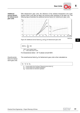
6Gear Units
Features The SEW geared motor forms a structural unit consisting of one of the previously
mentioned electric motors and a reduction gear unit. Criteria for the selection of a
suitable type of gear include availability of space, possibilities of mounting and
connection to the driven machine. The product range includes helical gear units, parallel
shaft helical gear units, helical bevel gear units in normal and low-backlash design, as
well as helical-worm gear units, Spiroplan®
gear units, planetary gear units and low-
backlash planetary gear units.
Helical gear units
with extended
bearing housing
Helical gear units with extended bearing housing represent a special design. It is
designated as RM and predominantly used for agitator applications. RM gear units are
designed for extremely high overhung and axial loads as well as flexural torque. The
remaining data is identical to the standard helical gear units.
Multi-stage gear
units
Multi-stage gear units may be used for particularly low output speeds by mounting a
suitable helical gear unit in the modular system at the input side.
Output speed,
output torque
The gear unit size depends on the output torque. This output torque Ma is calculated
based on the motor output power PN and the gear unit output speed na.
Specifying the
geared motor
The SEW geared motors listed in the catalog are described by the output power or
output torque at a given output speed. The service factor is an additional parameter.
PN = rated motor power [kW]
na = output speed of the gear unit [min –1
]
η = gear unit efficiency
1
2
3
4
5
6
7
8
9
10
11
12
13
14
15
16
17
18
6
48 Practical Drive Engineering – Project Planning of Drives
Gear Units
Gear unit
efficiency
Losses Typical losses in reduction gear units include frictional losses on meshing, in the
bearings and the oil seals, as well as oil churning losses involved in lubrication. Greater
losses occur with helical-worm gear units and Spiroplan® gear units.
The higher the gear unit input speed, the higher the losses.
Gearing efficiency The gearing efficiency is between 97 % and 98 % with helical, parallel shaft helical,
helical bevel and planetary gear units. With helical-worm and Spiroplan®
gear units, the
gearing efficiency is between 30 % and 90 %, depending on the design. During the run-
in phase, the efficiency of helical-worm and Spiroplan®
gear units may be up to 15 %
less. If this efficiency is below 50 %, the gear unit is statically self-locking. Such drives
may only be implemented if restoring torques do not occur, or if they are so small that
the gear unit cannot be damaged.
Oil churning
losses
The first gear unit stage completely immerses in the lubricant with certain mounting
positions. With larger gear units and high circumferential velocity of the input side, the
resultant oil churning losses reach a level that cannot be neglected.
Keep oil churning
losses at a
minimum
If possible, use the basic mounting position M1 for helical bevel, parallel shaft helical,
helical and helical-worm gear units to keep oil churning losses at a minimum.
Permitted
mountable
mechanical
power
Depending on application conditions (installation site, cyclic duration factor, ambient
temperature, etc.), gear units with critical mounting position and high input speed must
be checked to determine the amount of mechanical power that can be mounted. In these
cases, please consult SEW.
Practical Drive Engineering – Project Planning of Drives 49
6Gear Units
6.2 Dimensioning of standard gear units with service factor
The gear units are usually designed for uniform load and only a few starts/stops. If
deviations from these conditions exist, it is necessary to multiply the calculated
theoretical output torque or output power by a service factor. This service factor is
determined by the starting frequency, the mass acceleration factor and the daily
operating time. The following diagrams can be used as a first approximation.
In the case of characteristics specific to an application, higher service factors can be
determined referring to pragmatical values. The gear unit can be selected from the
output torque thus calculated. The permitted gear unit output torque must be greater or
equal to the calculated torque.
00656CXX
Figure 24: Required service factor fB for R, F, K, W, S gear units
04793AXX
Figure 25: Required service factor fB for P gear units
tB = operating time in hours per day [h/d]
c/h = cycles per hour
All start-ups and brake actions as well as the speed changes from high to low speed and vice versa must
be included in the number of starts and stops.
0 200 400 600 800 1200 14001000
24 16 8
tB [h/d]
0.8
0.9
1.0
1.1
1.2
1.3
1.4
1.5
1.6
1.0
1.1
1.2
1.3
1.4
1.5
1.6
1.7
1.2
1.3
1.4
1.5
1.6
1.7
1.8
c/h
fB
I
II
III
1
2
3
4
5
6
7
8
9
10
11
12
13
14
15
16
17
18
6
50 Practical Drive Engineering – Project Planning of Drives
Gear Units
Load
classification
I uniform, permitted mass acceleration factor ≤ 0.2
II non-uniform, permitted mass acceleration factor ≤ 3
III highly non-uniform, permitted mass acceleration factor ≤ 10
Example Load classification I with 200 starts and stops per hour and an operating time of 24 hours
a day gives fB = 1.35.
Service factor
fB > 1.8 Service factors > 1.8 can occur for some applications. These are caused by mass
acceleration factors > 10, by great backlash in the transmission elements of the driven
machine or by large overhung loads. In such cases, please consult SEW.
Determining the
load classification
The load classifications I to III are selected on the basis of the most unfavorable value
of the moments of inertia, external as well as on the motor side. It is possible to
interpolate between characteristics I to III.
SEW service factor The service factor for each geared motor is given in the SEW catalog. The service factor
represents the ratio of the rated gear unit power to the rated motor power. The
determination of the service factor is not standardized. For this reason, the specified
service factors are dependent on the manufacturer and cannot be compared.
fa = mass acceleration factor
JX = all external moments of inertia
JM = moment of inertia on the motor side
Practical Drive Engineering – Project Planning of Drives 51
6Gear Units
Additional
service factors
for helical-worm
gear units
With helical-worm gear units, the influence of the ambient temperature and cyclic
duration factor must also be taken into account when deciding on the gear unit. The
following figure illustrates the additional service factors for helical-worm gear units.
For temperatures below – 20 °C please consult SEW.
Overall service
factor for helical-
worm gear units
The overall service factor fBT for helical-worm gear units is then calculated as:
00657DXX
Figure 26: Additional service factors fB1 and fB2 for helical-worm gear units
fB2
-20 0-10 200 4010 6020 8030 100 % ED40 °C
fB1 I
II
III
1.0 0.6
1.2 0.8
1.4 1.0
1.6
1.8
CDF= cyclic duration factor
tB = time under load in min/h
fB = service factor from the figure "Required service factor fB"
fB1 = service factor from ambient temperature
fB2 = service factor for short-term operation
1
2
3
4
5
6
7
8
9
10
11
12
13
14
15
16
17
18
6
52 Practical Drive Engineering – Project Planning of Drives
Gear Units
6.3 Gear units for servo drives
Geared servomotors consist of synchronous or asynchronous servomotors in
combination with:
• Standard gear units: helical gear unit R series, parallel shaft helical gear units F
series, helical bevel gear units K series, helical-worm gear units S series
• Reduced backlash gear units: helical gear unit R series, parallel shaft helical gear
units F series, helical bevel gear units K series
• low backlash planetary gear units PS series.
Additional information can be found in the "Geared Servomotors" catalog.
Low backlash
planetary geared
motors
• Low backlash planetary geared motors PSF series
The PSF series is offered in gear unit sizes 211/212 to 901/902. It is characterized
by a B5 square flange with solid output shaft.
• Low backlash planetary geared motors PSB series
The PSB series is offered in gear unit sizes 311/312 to 611/612. The specific output
flange shaft meets EN ISO 9409. This standard covers the requirements for industrial
robots. The PSB series is increasingly used in industrial applications, which require
high overhung loads and high pull-out rigidity.
• Low backlash planetary geared motors PSE series
The PSE series is offered in gear unit sizes 211/212 to 611/612. It is characterized
by a round B14 flange with solid output shaft. The PSF gear unit series differs from
the existing PSF series through its more economical design. The technical data, such
as circumferential backlash, torque and reduction ratios, are comparable to those of
PSF/PSB gear units.
Dimensioning
information
The following data are required for dimensioning of geared servomotors:
– Output torque Mamax
– Output speed namax
– Overhung loads / axial loads FRa / FAa
– Torsion angle α < 1’, 3’, 5’, 6’, 10’, > 10’
– Mounting position M1 ... M6
– Ambient temperature ϑamb
– Exact load cycle, i.e. information on all required torques and activity times as well
as external moments of inertia to be accelerated and decelerated.
Practical Drive Engineering – Project Planning of Drives 53
6Gear Units
Gear unit backlash
N and R
PS. gear units are optionally designed with gear unit backlash N (normal) or R
(reduced).
Torsion angle < 1’ upon request
Motor support If large motors are mounted at PS. gear units, a motor support is required starting at the
following inertia forces:
PS. single stage: mM / mPS. > 4
PS. two-stage: mM / mPS. > 2.5
Additional project planning information for PS. gear units can be found in the "Low
Backlash Planetary Gear Units" and "Geared Servomotors" catalogs.
Reduced
backlash geared
servomotors
R/F/K
Reduced backlash helical-bevel, parallel shaft helical and helical geared motors with
synchronous or asynchronous servomotors in the speed range of
Mamax = 200 ... 3000 Nm complete the program of low backlash planetary geared
motors with limited circumferential backlash.
The reduced backlash designs are available for the following gear unit sizes:
• R37 ... R97
• F37 ... F87
• K37 ... K87
Project planning The connection dimensions and reduction ratio ranges are identical with those of the
standard designs.
The circumferential backlashes are listed in the corresponding catalogs in relation to the
gear unit size.
Gear units N R
PS. 211 ... 901 α < 6’ α < 3’
PS. 212 ... 902 α < 10’ α < 5’
1
2
3
4
5
6
7
8
9
10
11
12
13
14
15
16
17
18
6
54 Practical Drive Engineering – Project Planning of Drives
Gear Units
6.4 Overhung loads, axial loads
Additional criteria in selecting the gear unit size are the anticipated overhung loads and
axial loads. The shaft strength and bearing load capacity are decisive with respect to the
permitted overhung loads. The maximum permitted values given according to the
catalog always refer to the force acting at the midpoint of the shaft end in the most
unfavorable direction.
Point of
application
When the force is not acting at the midpoint, it results in permitted overhung loads which
are smaller or greater. The closer the point of application to the shaft shoulder, the
greater the permitted overhung loads that may be applied and vice versa. Please refer
to the "Geared Motors" catalog, "Project Planning of Gear Units," for the formulae for
eccentric action of force. You cannot calculate the permitted value of the axial load
unless you know the overhung load.
When the output torque is transmitted by means of a chain sprocket or gear wheel, the
overhung load at the shaft end is determined by the output torque and the radius of the
chain sprocket or gear wheel.
Determining the
overhung load
Additional overhung load factors fZ must be taken into account when determining the
overhung load. These depend on the method of transmission, i.e. gear wheels, chains,
V belt, flat belt or toothed belt. The belt pre-tensioning is an additional factor with belt
pulleys. The overhung loads calculated with the additional factor must not be greater
than the permitted overhung load for the gear units.
F = overhung load [N]
M = output torque [Nm]
r = radius [m]
Transmission element Transmission element factor fZ Comments
Direct drive 1.0 –
Gear wheels 1.0 ≥ 17 teeth
Gear wheels 1.15 < 17 teeth
Chain sprockets 1.0 ≥ 20 teeth
Chain sprockets 1.25 < 20 teeth
Narrow V-belt 1.75 Effect of pre-tensioning force
Flat belt 2.50 Effect of pre-tensioning force
Toothed belt 1.50 Effect of pre-tensioning force
Gear rack 1.15 < 17 teeth (pinion)
Practical Drive Engineering – Project Planning of Drives 55
6Gear Units
Definition of force
application
The force application is defined according to the following illustration:
FR = overhung load [N]
Md = output torque [Nm]
d0 = mean diameter [mm]
fZ = transmission element factor
02355CXX
Figure 27: Definition of force application
FX = permitted overhung load at point X [N]
FA = permitted axial load [N]
α α
0° 0°
x
FX
FA
- +
1
2
3
4
5
6
7
8
9
10
11
12
13
14
15
16
17
18
7
56 Practical Drive Engineering – Project Planning of Drives
Drive Engineering Formulae
7 Drive Engineering Formulae
7.1 Basic motions
All applications can be divided into two basic motions:
Kinematic
relationships
The following applies to linear motion:
Linear motion (travel drive, drive unit for vertical
motion)
Rotating motion (rotary table)
Distance s [m] Angular distance ϕ [rad] or [°]
rad is the radian measure
in a standard circle and
features no unit [rad] = 1
360 ° ‫־‬ 6.28 rad
Velocity v [m/s] Angular velocity ω [rad/s] or [1/s]
Speed n [min–1]
ω = 2 · π · n
Acceleration a [m/s2
] Angular acceleration α [rad/s2
] or [1/s2
]
Force F [N] Torque M [Nm]
Weight m [kg] Moment of inertia J [kgm2
]
Radius
Diameter
r [m]
D [m]
v = const. a = const.
Distance
Velocity
Acceleration
Time
Practical Drive Engineering – Project Planning of Drives 57
7Drive Engineering Formulae
The following applies to rotation:
Conversion of
linear and
rotating motion
Since the basic motion of a geared motor is always a rotation, regardless of the
application, every linear motion must first be converted into a rotating motion and vice
versa.
ω = const. α = const.
Distance
Velocity
Acceleration
Time
Angle
Velocity
Acceleration
1
2
3
4
5
6
7
8
9
10
11
12
13
14
15
16
17
18
7
58 Practical Drive Engineering – Project Planning of Drives
Drive Engineering Formulae
7.2 Moments of inertia
Reduction of
external
moments of
inertia
All moments of inertia to be accelerated must be referenced to the motor shaft and
added to calculate the starting and braking behavior of a drive. All gear ratios are
entered in square manner In accordance with the energy conservation law.
This results in the following application for a rotating motion:
In the same way, a mass m conveyed in a linear direction can also be reduced to the
motor shaft:
External moment
of inertia
JL = moment of inertia of the load
JX = external moment of inertia reduced to motor shaft
iT = total gear ratio
Rotation
n = speed after total gear ratio (additional gear and gear unit)
nM = motor speed
Linear motion
Practical Drive Engineering – Project Planning of Drives 59
7Drive Engineering Formulae
Rotating bodies Moments of inertia of typical rotating bodies
Body Position of rotary axis Symbol Moment of inertia J
Ring, thin hollow
cylinder, thin-walled
vertical to ring plane
Solid cylinder its longitudinal axis
Hollow cylinder, thick-
walled
its longitudinal axis
Disc vertical to disc plane
Disc
symmetry axis in disc
plane
Sphere
axis through mid-
point
Sphere, thin-walled
axis through mid-
point
Rod, thin with length l
vertical to middle of
rod
A
S
a
Steiner’s law
JS = Moment of inertia of a body in reference to an axis of rotation passing through the center of
gravity S
JA = moment of inertia of the same body in reference to an axis of rotation through A
a = distance between the two axes running parallel to each other
m = weight of the body
1
2
3
4
5
6
7
8
9
10
11
12
13
14
15
16
17
18
7
60 Practical Drive Engineering – Project Planning of Drives
Drive Engineering Formulae
7.3 Static or dynamic power
The total power of each application is divided into static and dynamic power. The static
power is the power at constant speed, primarily friction forces and gravitational forces.
Dynamic power is the power required for acceleration and deceleration. Both power
components exert different influences with different applications.
Horizontal /
vertical
This relationship is explained by means of the vertical and horizontal motions.
For a better comparison base, we are assuming identical values for mass, speed and
acceleration.
This example shows that a hoist drive requires more power overall than a travel drive.
In addition, 90% of the motor size of a hoist drive is determined by the gravitational force
and, therefore, by the static power.
In comparison, 90% of the motor size of a travel drive is determined by the acceleration
force and, therefore, by the dynamic power.
Hoist drive with
counterweight
Yet another application is a hoist drive with counterweight. The gravitational force
becomes zero with 100 % weight compensation, but the acceleration power doubles
since the weight has been doubled. However, the total power is less than that of a hoist
drive without counterweight.
Force Vertical motion Horizontal motion
Gravitational force large zero
Acceleration force same size
Friction force neglected in this example
m m
Practical Drive Engineering – Project Planning of Drives 61
7Drive Engineering Formulae
7.4 Resistance forces
Resistance forces are forces counteracting the motion.
Static resistance
forces
Static and sliding friction
The resistance to motion consists of:
Gravitational forces
Friction force
FR = friction force [N]
µ = friction factor
FN = weight perpendicular to the surface [N]
Weight
m = mass [kg]
g = gravitational acceleration [m/s2
]
α = lead angle [°]
Resistance to
motion
FF = resistance to motion [N]
D = diameter of traveling wheel [mm]
µL = bearing friction factor
d = bearing diameter [mm]
f = lever arm of rolling friction [mm]
c = wheel flange and rim friction
Rolling friction
Bearing friction
Track friction
Vertical hoist
drive
Gravity
resistance
1
2
3
4
5
6
7
8
9
10
11
12
13
14
15
16
17
18
7
62 Practical Drive Engineering – Project Planning of Drives
Drive Engineering Formulae
Dynamic
resistance forces
Acceleration force
7.5 Torques
7.6 Power
7.7 Efficiencies
The total efficiency of the system is composed of the multiplication of all individual
efficiencies in the drive train. In general, these are:
• Gear unit efficiency ηG
• Load efficiency ηL
Overall efficiency ηT = ηG · ηL
This overall efficiency must be considered separately for static and for dynamic power.
Linear motion
Rotation
Linear motion
Rotation
Linear motion
Rotation
Practical Drive Engineering – Project Planning of Drives 63
7Drive Engineering Formulae
7.8 Spindle calculation
Dynamic torques are calculated using the formulae of the linear motion.
Spindle speed
n = spindle speed
v = speed of load
P = spindle pitch
Angular distance
ϕ = angular distance of the
spindle
s = distance of the load
P = spindle pitch
Angular
acceleration
α = angular acceleration of the spindle
a = acceleration of the load
P = spindle slope
Static torque
F = resistance force of the load, e.g. through friction
P = spindle slope
M = static torque
η = spindle efficiency (see appendix with tables)
1
2
3
4
5
6
7
8
9
10
11
12
13
14
15
16
17
18
7
64 Practical Drive Engineering – Project Planning of Drives
Drive Engineering Formulae
7.9 Special formulae
See the legend regarding explanations of the individual symbols.
Size Horizontal and rotating motion, vertical
motion upward
Vertical motion downward (simplified
calculation with synchronous speed)
Run-up time [s]
Switching time [s]
Braking time [s]
Start-up distance
[mm]
Switching
distance [mm]
Braking distance
[mm]
Braking accuracy
Start-up
acceleration
[m/s2]
Switching time
lag [m/s2
]
Braking
deceleration
[m/s2]
Starting
frequency [c/h]
Braking energy
[J]
Brake service life
[h]
Practical Drive Engineering – Project Planning of Drives 65
8Calculation Example: Travel Drive
8 Calculation Example: Travel Drive
Input data An AC brake motor with helical gear unit must be dimensioned using the following data:
Two wheels are driven; the wheels must not slip at start-up.
Mass of traveling vehicle: m0 = 1,500 kg
Additional load: mL = 1,500 kg
Velocity: v = 0.5 m/s
Wheel diameter: D = 250 mm
Axle diameter: d = 60 mm
Friction surfaces: steel/steel
Lever arm of the rolling friction: steel on steel f = 0.5 mm
Factors for rim friction and wheel flange
friction:
for anti-friction bearings c = 0.003
Factors for bearing friction: for anti-friction bearings µL = 0.005
Additional gear: Chain reduction, iV = 27/17 = 1.588
Sprocket diameter (driven): d0 = 215 mm
Load efficiency: ηL = 0.90
Cyclic duration factor: 40 % CDF
Starting frequency: 75 cycles/hour loaded and 75 travels/hour
unloaded, 8 hours/day
00777AXX
Figure 28: Travel drive
1
2
3
4
5
6
7
8
9
10
11
12
13
14
15
16
17
18
8
66 Practical Drive Engineering – Project Planning of Drives
Calculation Example: Travel Drive
8.1 Motor calculation
The number of running wheels is irrelevant for the calculation of the resistance to
motion.
Static power The static power PS takes into account all forces that occur when the drive is not
accelerated, such as:
– rolling friction
– friction forces
– hoisting force on a slope
– wind power
Efficiency ηT is the total efficiency of the drive system consisting of the gear unit efficiency ηG and
the efficiency of external transmission elements ηL. The efficiency of the transmission
elements is given in the appendix with tables.
Helical and helical-
bevel gearing
The gear unit efficiency of helical and helical-bevel gearing can be assumed at ηG = 0.98
per gear wheel stage (e.g. 3-stage gear unit ηG = 0.94). Please refer to the SEW Geared
Motors catalog for the efficiency of helical-worm gear units, taking the gear ratio into
account.
As type and size of the gear unit have not yet been defined, the mean value of 2- and
3-stage gear units ηG = 0.95 is used for calculation.
Load efficiency The load efficiency is dependent on the transmission elements installed behind the gear
unit (e.g. chains, belts, ropes, gearing parts, etc.).
From appendix with tables: Efficiency of chains ηL = 0.90 ... 0.96.
The smallest value (ηL = 0.90) is used for calculation if more detailed values are not
available.
Resistance to
motion
loaded
unloaded
Overall efficiency
Practical Drive Engineering – Project Planning of Drives 67
8Calculation Example: Travel Drive
Retrodriving
efficiencies
Retrodriving efficiencies can be calculated according to the following formula:
This shows that the retrodriving efficiency becomes equal to zero (static self-locking!)
with an efficiency of 50 % (0.5) or less.
Static power
The calculated static power refers to the motor shaft.
This power is only one part of the required motor power, since the acceleration power
(= dynamic power) is decisive for horizontal drive systems.
Dynamic power The dynamic power is the power which accelerates the complete system (load,
transmission elements, gear unit and motor). The motor provides a starting torque with
uncontrolled drive systems which accelerates the system. The greater the starting
torque, the greater the acceleration.
In general, the moments of inertia of transmission elements and gear units can be
ignored. The moment of inertia of the motor is not yet known, as the motor is yet to be
dimensioned. For this reason, a motor must first be approximately calculated on the
basis of the dynamic power for accelerating the load. Since the ratio of the moment of
inertia of the load and of the motor is normally very high in travel drives, the motor can
be determined very exactly at this point already. It is still necessary to make further
checks.
The missing value of the permitted starting acceleration aP is yet to be calculated. It is
important to ensure that the wheels are not spinning .
loaded
unloaded
Overall power
PT = overall power
PDL = dynamic power of the load
PDM = dynamic power of the motor
PS = static power
η = overall efficiency
1
2
3
4
5
6
7
8
9
10
11
12
13
14
15
16
17
18
8
68 Practical Drive Engineering – Project Planning of Drives
Calculation Example: Travel Drive
Permitted starting
acceleration
The wheels slip as soon as the peripheral force FU on the wheel becomes greater than
the friction force FR.
m’ = mass lying on the driving wheels, with 2 driven wheels is m’ = m/2
µ0 = 0.15 (static friction steel/steel, see appendix with tables)
If the acceleration a is smaller than the permitted acceleration aP, the wheels do not slip.
Overall power (without dynamic power of the motor)
Smooth
acceleration
A 2-pole motor was selected to prevent slipping of the running wheels due to excessive
acceleration. More energy is required to accelerate the motor to the high speed due to
the lower ratio of the external moment of inertia and the motor moments of inertia. The
acceleration process is smoother.
Acceleration
torque
With 2-pole motors of this power range, the starting torque MH is twice as high as the
rated torque. As the specified acceleration represents the maximum permitted
acceleration, we first select a motor with a power rating that is less than the total power
Ptot calculated for the unloaded status.
Peripheral force
Borderline
case:
Permitted
acceleration
loaded
unloaded
Selected motor: DT71D2 /BM
Data from "Geared Motors" catalog
PN = 0.55 kW
nN = 2,700 min–1
MH/MN = 1.9
JM = 5.51 · 10–4
kgm2
Practical Drive Engineering – Project Planning of Drives 69
8Calculation Example: Travel Drive
Calculation check So far, the calculation was carried out without motor data. For this reason, detailed
checking of the calculation data is required using the motor.
Start-up behavior External moment of inertia converted with reference to the motor shaft without load:
Torques
Run-up time unloaded
Start-up acceleration unloaded
The starting acceleration without load is extremely high. The acceleration can be
reduced with an increased moment of inertia of the motor, e.g. by mounting a flywheel
fan. This setup reduces the maximum permitted starting frequency. The acceleration
can also be reduced by selecting a smaller motor.
External moment of
inertia
Rated torque
Acceleration torque
MH is no catalog value and
must be converted.
Load torque
unloaded
ML is a pure calculation
factor without efficiency.
Load torque loaded
1
2
3
4
5
6
7
8
9
10
11
12
13
14
15
16
17
18
8
70 Practical Drive Engineering – Project Planning of Drives
Calculation Example: Travel Drive
Flywheel fan Repeated checking without load with flywheel fan (JZ = 0.002 kgm2
):
The starting acceleration without load is in the permitted range, i.e. a suitable motor has
been found.
Accleration time and starting acceleration with load
Acceleration time
Start-up acceleration
Acceleration time
Start-up acceleration
Start-up distance
Practical Drive Engineering – Project Planning of Drives 71
8Calculation Example: Travel Drive
Permitted starting
frequency
The permitted starting frequency for the combination of an equal number of cycles with
and without load per cycle can be determined with the following formula:
The requirement of 75 cycles per hour can be met.
loaded
no-load starting frequency of the motor according to catalog with BGE brake rectifier.
unloaded
loaded and unloaded
ZC = starting frequency per cycle
ZPL = permitted starting frequency unloaded
ZPE = permitted starting frequency loaded
1
2
3
4
5
6
7
8
9
10
11
12
13
14
15
16
17
18
8
72 Practical Drive Engineering – Project Planning of Drives
Calculation Example: Travel Drive
Braking behavior
Braking torque The absolute values of acceleration and deceleration should be similar. It is important
to keep in mind that the resistance to motion and thus the resulting load torque support
the braking torque.
Braking torque
Braking time
Braking deceleration
rate
Braking distance
t2 = t2II = 0.005 s for switching in the DC and AC circuit of the brake (see "Geared Motors" catalog, chapter
on AC brake motors).
Braking accuracy
Practical Drive Engineering – Project Planning of Drives 73
8Calculation Example: Travel Drive
Braking energy The braking energy is converted into heat in the brake lining and is a measure for the
wear of the brake linings.
The travel vehicle travels alternatingly loaded and unloaded, so that the average of the
braking energy WB must be assumed when calculating the brake service life.
After a maximum of 2,600 operating hours (corresponds to approx. 1 year at 8 hours/
day), the brake must be readjusted and the brake disc must be checked.
8.2 Gear unit selection
loaded
unloaded
Braking energy
Brake service life
WN = rated braking energy
(see appendix with tables)
Output speed
Gear unit ratio
1
2
3
4
5
6
7
8
9
10
11
12
13
14
15
16
17
18
8
74 Practical Drive Engineering – Project Planning of Drives
Calculation Example: Travel Drive
Service factor With 8 hours/day operation and 150 cycles/hour, i.e. 300 starts and stops per hour, the
following service factor is determined using "Required service factor fB" in the chapter
on "Gear Units:"
With a mass acceleration factor > 20, which is quite common with travel drives, it is
important to ensure that the drive system has as little backlash as possible. Otherwise
the gear units might be damaged when operated at the supply.
Reference power The reference power for the calculation of the gear unit is generally the rated motor
power.
Suitable gear unit: R27 with na = 60 min–1
and Mamax = 130 Nm
Consequently, the output torque Ma (referred to the motor rated power), the service
factor fB and the overhung load FQ are:
Number of teeth < 20, subsequently fZ = 1.25 (see appendix with tables "Overhung
Loads, Axial Loads")
With belt drive systems, the pre-tensioning must also be observed: FRa_perm = 3,530
Nm.
The recommended drive system is: R27DT71D2 /BMG.
⇒ load classification 3
Output torque
Output torque
Service factor
Overhung load
Practical Drive Engineering – Project Planning of Drives 75
8Calculation Example: Travel Drive
8.3 Travel drive with two speeds
The travel drive of the previous example is to travel with a quarter of the speed in setup
mode (8/2-pole motor). In addition, the stopping accuracy is to be reduced to ± 5 mm.
The static relations remain the same.
Input data Mass of traveling vehicle: m0 = 1,500 kg
Additional load: mL = 1,500 kg
Velocity: v = 0.5 m/s
Wheel diameter: D = 250 mm
Adopted from the previous example:
Resistance to motion: FF = 241 N
Static power: Pstat = 0.14 kW
Overall efficiency: ηT = 0.85
Switching time lag The procedure is identical to the previous example. The critical point is not the starting
acceleration but the switching time lag from high to low speed when operating multi-
speed motors. Multi-speed motors provide approximately 2.5 times the starting torque
in the "slow winding" as switching torque.
The starting torque in the "slow winding" is approximately 1.7 times the rated torque for
motors of the anticipated power range. Thus, the anticipated switching torque is
approximately
Motor selection For this reason, we are selecting a motor with an 8-pole rated power that is at least 4.25
times less the dynamic power calculated from the load at the permitted acceleration.
Switching torque
MN8P= rated torque of the 8-pole winding
Dynamic power
Total power
Selected motor: DT71D8/2 /BM
Data from "Geared Motors" catalog
PN = 0.06/0.25 kW
nN = 675/2,670 min–1
MH/MN = 1.4/1.8
JM = 5,3 · 10–4
kgm2
1
2
3
4
5
6
7
8
9
10
11
12
13
14
15
16
17
18
8
76 Practical Drive Engineering – Project Planning of Drives
Calculation Example: Travel Drive
Rated motor torque for the 2-pole speed
Switching time lag The decisive factor for multi-speed is the switching time lag:
Rated torque
Acceleration torque
Load torque
ML is a pure calculation factor
without efficiency.
External moment of
inertia
Acceleration time
Start-up acceleration
Switching time
Switching torque
Switching time
Switching
acceleration
Practical Drive Engineering – Project Planning of Drives 77
8Calculation Example: Travel Drive
When switching without load, the value is 1.22 m/s2
. However, as already calculated in
the previous example, the maximum permitted acceleration is aP = 0.74 m/s2
. There are
two possibilities to improve the switching behavior as described in the following
sections.
Flywheel fan The flywheel fan prolongs the switching time due to its high rotating masses. The
permitted starting frequency, however, is considerably reduced.
Smooth pole-
change unit (WPU)
The WPU device utilizes the switching torque reduction (by approx. 50 %) of two-phase
switching. The third phase is automatically reconnected.
We select the solution with WPU, as we do not want to accept a reduction of the starting
frequency. In extreme cases it is also possible to combine both elements.
In the case of unloaded travel, the values are:
Switching time
Switching
acceleration
Permitted starting
frequency loaded
1
2
3
4
5
6
7
8
9
10
11
12
13
14
15
16
17
18
8
78 Practical Drive Engineering – Project Planning of Drives
Calculation Example: Travel Drive
Additional heat
generation during
switching
A factor of 0.7 must be considered in the calculation due to the additional heat generated
during the switching process. Subsequently, the drive is able to move the fully loaded
vehicle with the starting frequency ZPL = 180 · 0.7 = 126 times.
The permitted starting frequency increases when the motor has been designed in
thermal classification H or if it is equipped with a flywheel fan.
A further possibility of increasing the permitted starting frequency is to start-up the drive
at a low velocity (in the higher-pole winding).
The calculated starting frequency is increased by approx. 25 % when starting at low
speed and subsequently switching to high speed.
In this case, however, an additional load impact occurs which is not desirable in some
applications. Furthermore, the cycle time increases.
Starting
frequency of
several cycles
The vehicle travels loaded in one direction and returns unloaded. The permitted starting
frequency with load was calculated at 126 c/h. The starting frequency without load can
now be calculated with the previous formulae and the no-load weight.
The motor reaches the thermal utilization after 126 c/h with load or 320 c/h without load.
Resistance to motion
Static torque
ML is a pure calculation
factor without efficiency.
Permitted starting
frequency
Practical Drive Engineering – Project Planning of Drives 79
8Calculation Example: Travel Drive
To express this value in cycles, a mean value must be calculated using the following
formula.
More than two
types of load
The individual cycles must be converted into corresponding no-load cycles in case there
are more than two different types of load.
Assumption The vehicle travels along an inclined plane.
The cycle is:
1. travel with load up
2. travel with load down
3. travel with load up
4. travel without load down
The cycle then re-starts at the beginning.
Values for the
starting
frequencies
The values are selected at random.
No-load starting
frequency
According to the catalog, the permitted no-load starting frequency of the motor is 1,200
c/h.
First of all, the number of no-load cycles equivalent to one load cycle is calculated in the
corresponding travel type.
In words: Of the 1,200 c/h that the motor can start-up without load, 58.6 no-load cycles are "used
up" during one cycle.
This means that it is possible to travel 1,200/58.6 = 20.5 cycles per hour.
Permitted starting
frequency
Starting frequency With load up With load down Without load up Without load
down
Starting frequency [c/h] 49 402 289 181
1,200/49 = 24.5 with load up (24.5 no-load cycles correspond to one load
cycle)
+ 1,200/402 = 3.0 with load down
+ 1,200/49 = 24.5 with load up
+ 1,200/181 = 6.6 without load down
58.6
1
2
3
4
5
6
7
8
9
10
11
12
13
14
15
16
17
18
8
80 Practical Drive Engineering – Project Planning of Drives
Calculation Example: Travel Drive
Calculation of the
stopping
accuracy
The calculations refer to the travel with load, as the braking distance is greater, i.e. the
drive does not stop as accurately in this case as it does when traveling unloaded.
Braking torque The braking torque is specified at 2.5 Nm as in the previous example.
Braking time
Braking deceleration
rate
Braking distance
t2 = t2II = 0.005 s for switching in the DC and AC circuit of the brake.
Stopping accuracy
Practical Drive Engineering – Project Planning of Drives 81
8Calculation Example: Travel Drive
8.4 Travel drive with frequency inverter
Input data A vehicle with a no-load weight of m0 = 500 kg is to carry an additional load of mL = 5 t
over a distance of sT = 10 m in tT = 15 s. On the way back, the vehicle travels without
load at twice the speed.
The acceleration is set at a = 0.5 m/s2
are specified. In addition, 0.5 s positioning travel
must be included after the deceleration ramp in order to improve the stopping accuracy.
00780AXX
Figure 29: Travel cycle
Wheel diameter: D = 315 mm
Axle diameter: d = 60 mm
Friction surfaces: steel/steel
Lever arm of the rolling friction: steel on steel f = 0.5 mm
Factors for rim friction and wheel flange
friction:
for anti-friction bearings c = 0.003
Factors for bearing friction: for anti-friction bearings µL = 0.005
Additional gear: Chain reduction, iV = 27/17 = 1.588
Sprocket diameter (driven): d0 = 215 mm
Load efficiency: ηL = 0.90
Gear unit efficiency: ηG = 0.95.
Cyclic duration factor: 60 % CDF
Additonal overhung load factor: fZ = 1.25
Setting range: 1 : 10
Starting frequency: 50 cycles/hour
1
2
3
4
5
6
7
8
9
10
11
12
13
14
15
16
17
18
8
82 Practical Drive Engineering – Project Planning of Drives
Calculation Example: Travel Drive
Optimizing the
travel cycle
Optimization for minimum acceleration:
Optimization for velocity: The acceleration is given.
00781AXX
Figure 30: Optimization for acceleration
00782AXX
Figure 31: Optimization for velocity
Practical Drive Engineering – Project Planning of Drives 83
8Calculation Example: Travel Drive
Positioning time Even though the positioning time is neglected, the result is sufficiently exact.
This step concludes the calculation of the travel cycle.
Velocity
Acceleration time
Run-up distance
Switching time
Switching distance
Positioning distance
Traveling distance
Traveling time
Total time
1
2
3
4
5
6
7
8
9
10
11
12
13
14
15
16
17
18
8
84 Practical Drive Engineering – Project Planning of Drives
Calculation Example: Travel Drive
Calculation of
power
Dynamic power without motor moment of inertia, for the estimation of the motor power:
Total power without acceleration power of the motor mass which is not yet known.
Since 150 % of the rated current can be provided for acceleration by the frequency
inverter, we select a 2.2 kW motor.
Resistance to motion
Static power
Load torque
ML is a pure calculation
factor without efficiency.
Dynamic power
Total power
Selected motor: DV100M4 /BMG
Data from "Geared Motors" catalogPN = 2.2 kW
nN = 1,410 min–1
JM = 59 · 10–4
kgm2
(incl. brake)
Practical Drive Engineering – Project Planning of Drives 85
8Calculation Example: Travel Drive
Acceleration power
This calculation example requires 132 % MN which is just about within the permitted
range.
Acceleration torque
External moment of
inertia
Acceleration torque
Rated torque
MH / MN
Since the output torque of the motor is not proportional to the motor current in the lower
speed range (< 25 % of the rated speed), a motor torque of 130 % MN at 150 % motor
current (adjusted inverter) is used for calculation.
1
2
3
4
5
6
7
8
9
10
11
12
13
14
15
16
17
18
8
86 Practical Drive Engineering – Project Planning of Drives
Calculation Example: Travel Drive
Setting range
Field weakening
range
If the motor is operated above the base frequency f1 (in the so-called field weakening
range), it is important to keep in mind that the rated torque decreasing in inverse
proportion as well as the quadratically decreasing pull-out torque are higher than the
required load torque.
Reduced speed in
the constant torque
range
Due to the reduced fan speed during operation at reduced speed, fan-cooled motors
cannot completely dissipate the developing heat. Detailed knowledge of the maximum
cyclic duration factor and the torque load in this range are the decisive factors for the
correct dimensioning in this case. In many cases, forced cooling or a larger motor, which
can dissipate more heat due to the larger surface, must be implemented.
Guidelines for
dimensioning in
the setting range
• At least thermal classification F
• Implement temperature sensors (TF) or bimetallic strips (TH) in the motor
• Use only 4-pole motors for speed range, efficiency η and cos ϕ
Detailed information on project planning can be found in "Drive-Engineering – Practical
Implementation – Frequency Inverters."
Field weakening
range
Since the load during the fast return travel is very low, the motor is operated at 100 Hz
in the field weakening range. This fact requires a torque check.
Rated motor torque at base frequency: MN = 15 Nm
Pull-out torque at base frequency: MK = 35 Nm
00783BXX
Figure 32: Field weakening range
[1] = field weakening range
f1 = base frequency
Practical Drive Engineering – Project Planning of Drives 87
8Calculation Example: Travel Drive
At 100 Hz
operation
The load torque at m0 = 500 kg (no-load cycle) is 0.22 Nm + 1.5 Nm = 1.72 Nm including
acceleration component and efficiency, i.e. operation in the field weakening range is
permitted.
The 87 Hz
characteristics
The next smaller motor can be selected for the previous example when using the 87 Hz
characteristics.
This motor can provide a power of 2.2 kW in continuous operation when implementing
the 87 Hz characteristics in connection with a 2.2 kW inverter.
The load torque in relation to the new rated speed nN = 2,440 min–1 is
ML = 1.16 Nm.
The new rated motor torque in relation to nN = 2,440 min–1
and PN = 2.2 kW is
MN = 8.6 Nm.
The 87 Hz characteristics is permitted.
Rated torque
Pull-out torque
Selected motor: DT 90 L4 BMG
Data from "Geared Motors" catalogPN = 1.5 kW at nN = 1,400 min–1
PN = 2.2 kW at nN = 2,440 min–1
JM = 39.4 · 10–4
kgm2
(incl. brake)
External moment of
inertia
Acceleration torque
MH / MN
1
2
3
4
5
6
7
8
9
10
11
12
13
14
15
16
17
18
8
88 Practical Drive Engineering – Project Planning of Drives
Calculation Example: Travel Drive
Speed control The characteristics of the AC motor in connection with a frequency inverter are improved
by the "speed control" option.
• The following components are also required:
– Incremental encoder mounted to the motor
– Speed controller integrated in the inverter
• The following drive-specific characteristics are achieved by speed control:
– Control range of the speed up to 1:100 at fmax = 50 Hz
– Load dependency of the speed < 0.3 % related to nN and step change in load ∆M
= 80 %
– Transient recovery time in case of load variation is reduced to approx. 0.3 ... 0.6 s
The motor can temporarily produce torques which exceed its pull-out torque at supply
operation with the corresponding inverter assignment. Maximum acceleration values
are reached in case the motor is dimensioned for fmax < 40 Hz and the base frequency
is set to 50 Hz.
Synchronous
operation
With the "synchronous operation" function, a group of asynchronous motors can be
operated angular synchronously to one another or in an adjustable proportional ratio.
• The following components are also required:
– Incremental encoder mounted to the motor
– Synchronous operation controller/speed controller integrated in the inverter
• The following tasks can be carried out:
– Angular synchronous operation of two to ten drives ("electric wave")
– Proportional operation (settable synchronous reduction ratio, "electronic gear
unit")
– Temporary synchronous operation with internal acquisition of the offset angle
during free-running ("flying saw")
– Synchronous operation with offset but without new reference point (torsion test
stand, generation of imbalance in vibrators)
– Synchronous operation with offset and new reference point (transfer conveyor)
Practical Drive Engineering – Project Planning of Drives 89
8Calculation Example: Travel Drive
"Flying saw" A constantly moving plastic rope is to be cut at an exact distance of one meter.
Input data Rate of feed: 0.2 m/s
Max. travel of the saw: 1 m
Weight of the saw: 50 kg
Duration of the sawing process: 1 s / 0.4 m
To simplify matters, the diameters of the sprocket wheels are identical (215 mm). The
conveyor belt is defined with R63 DT71D4 (i = 42.98) calculated for an inverter
frequency of 30 Hz. If possible, the same gear unit is to be implemented for feeding the
saw.
Explanation The 30 Hz of the conveyor belt were selected with identical gear unit reduction so that
the saw can catch up fast with the conveyor. This step is not absolutely essential. If
different gear ratios are selected, an adjustment in the synchronous operation
electronics can be programmed.
Process The complete synchronous sawing process is followed by a limited period in free-
running mode by the saw drive. The distance of the axes, however, is continuously
recorded. In addition, a so-called slave counter can be programmed. Using the
programmed number of pulses, this counter calculates a new reference point with an
offset equal to the sawing distance.
50306AXX
Figure 33: "Flying saw"
1
2
3
4
5
6
7
8
9
10
11
12
13
14
15
16
17
18
8
90 Practical Drive Engineering – Project Planning of Drives
Calculation Example: Travel Drive
The sawing axis uses the free-running period to return to a light barrier mounted at the
zero point disables free-running with a binary signal to the synchronous operation
controller. The sawing axis travels to the new reference point. The sawing process is
started by a programmable output relay in the inverter (in slave position).
The return distance (800 mm, 200 mm reserve) should be covered in two seconds.
Inverter frequency Using the known "Drive Engineering Formulae," the drive must travel at a speed of 0.55
m/s with an acceleration of 1 m/s2
which corresponds to an inverter frequency of:
00785BXX
Figure 34: Distance-time diagram of the "flying saw"
[1] = return travel
[2] = synchronous operation
Practical Drive Engineering – Project Planning of Drives 91
8Calculation Example: Travel Drive
Distance-time
diagram
This means that the same drive as the one used for the conveyor belt can be
implemented with the 87 Hz characteristics. The power is determined the same way it
has been done in the previous examples. Catching-up must be carried out within approx.
one second with the inverter traveling at fmax. The acceleration is defined by the set KP
control factor. Two seconds are left for sawing which still leaves some reserve.
As can be seen in the distance-time diagram, it is important for project planning that the
return travel should be ended before reaching the sawing mark to avoid unnecessarily
long catch-up distances.
1
2
3
4
5
6
7
8
9
10
11
12
13
14
15
16
17
18
9
92 Practical Drive Engineering – Project Planning of Drives
Calculation Example: Hoist Drive
9 Calculation Example: Hoist Drive
Input data Hoist drives require the major portion of their torque in non-accelerated (quasi-
stationary) state, i.e. only a small percentage of the torque is required for accelerating
the masses (exception: hoist drive with counterweight).
Use a multi-speed motor with a 4:1 speed ratio.
Weight of hoist frame: m0 = 200 kg
Weight of the load: mL = 300 kg
Hoisting speed: v = 0.3 m/s
Sprocket diameter: D = 250 mm
Load efficiency: ηL = 0.90
Gear unit efficiency: ηG = 0.95
Overall efficiency: η = ηL · ηG ≈ 0.85
Cyclic duration factor: 50 % CDF
One drive, direct drive
00786AXX
Figure 35: Hoist drive
Practical Drive Engineering – Project Planning of Drives 93
9Calculation Example: Hoist Drive
9.1 Multi-speed motor
The selected motor power should be greater than the calculated static (quasi-stationary)
power.
Due to the required power, the motor is selected at maximum speed. The speed ratio of
4:1 is ideal for a 8/2-pole motor.
Static power
Selected motor: DT100LS8/2 /BMG
PN = 0.45/1.8 kW
nM = 630/2,680 min–1
MH = 10.9/14.1 Nm
JM = 48.1 · 10–4
kgm2
Z0 = 2,600/9,000
MB = 20 Nm
MU = 2.5 · MH (8-pole) = 27.3 Nm
External moment of
inertia
Static motor torque
CAUTION!
The load supports the motor in downward motion and counteract it in upward motion.
Consequently, different formulae must be used in some cases for the following
calculations for vertical motion upward and downward (see the chapter on "Formulae of
Drive Engineering").
1
2
3
4
5
6
7
8
9
10
11
12
13
14
15
16
17
18
9
94 Practical Drive Engineering – Project Planning of Drives
Calculation Example: Hoist Drive
Upward motion
Starting time
Starting acceleration
Starting distance
Switching time from
2-pole to 8-pole
Switching time lag
Switching distance
Practical Drive Engineering – Project Planning of Drives 95
9Calculation Example: Hoist Drive
Braking power A speed change resulting from a "delay" must be taken into account for the calculation
of the braking power. This delay occurs between motor stopping and brake actuation.
Speed change and
delay
Braking time
Braking deceleration
Braking distance
Stopping accuracy
Calculation factor
static power and
cyclic duration factor
CDF
Starting frequency
1
2
3
4
5
6
7
8
9
10
11
12
13
14
15
16
17
18
9
96 Practical Drive Engineering – Project Planning of Drives
Calculation Example: Hoist Drive
Downward
motion
Since the motor is operated in regenerative mode, the motor speed with the
synchronous speed 3,000 min–1
and 750 min–1
is used for the calculation of the
downward travel.
Starting time
Starting acceleration
Starting distance
Switching time
Switching time lag
Switching distance
Braking time
Braking deceleration
Braking distance
Stopping accuracy
Practical Drive Engineering – Project Planning of Drives 97
9Calculation Example: Hoist Drive
The permitted number of cycles ZC is determined as follows:
The additional heat generated when switching from high to low speed reduces the
permitted starting frequency depending on the type of motor. In our case the reduction
factor is 0.7.
The result is a maximum of 196 cycles (upwards and downwards motion).
The calculation of the gear unit is carried out as shown in the previous example.
9.2 Motor with frequency inverter
Input data The hoist drive is to be equipped with a frequency-controlled drive.
Calculation factor
static power and
cyclic duration factor
CDF
Starting frequency
Number of cycles
Weight of hoist frame: m0 = 200 kg
Weight of the load: mL = 300 kg
Hoisting speed: v = 0.3 m/s
Sprocket diameter: D = 250 mm
Base frequency: f1 = 50 Hz
Max. frequency: fmax = 70 Hz
Acceleration/precontrol: a = 0.3 m/s2
Setting range: 1 : 10
Load efficiency: ηL = 0.90
Gear unit efficiency: ηG = 0.92
Overall efficiency: η = ηL · ηG ≈ 0.83
Cyclic duration factor: 50 % CDF
Gear unit: Helical bevel gear unit without
additional gear
1
2
3
4
5
6
7
8
9
10
11
12
13
14
15
16
17
18
9
98 Practical Drive Engineering – Project Planning of Drives
Calculation Example: Hoist Drive
Static power The selected motor power should be greater than the calculated static (quasi-stationary)
power.
Determining the
motor
Assuming that the dynamic power of hoists without counterweight is considerably small
(< 20 % of the static power), the motor can be determined by calculating PS.
Static power PS = 1.77 kW
Selected motor PN = 2.2 kW
Inverter PN = 2.2 kW
Thermal
considerations
For thermal reasons and due to improved magnetization, we recommend selecting the
motor for hoisting applications one type size larger. This holds especially true in case
the static power reaches the rated motor power level. In the present example, the
difference is large enough so that the motor does not need to be overdimensioned.
Motor selection The following motor was selected based on these conditions:
Hoisting applications operated on a frequency inverter should generally be
dimensioned for a maximum frequency of 70 Hz. If the drive reaches the maximum
speed at 70 Hz instead of 50 Hz, the gear ratio and thus the torque ratio increases by a
factor of 1.4 (70/50). If the base frequency is now set to 50 Hz, the output torque
increases by factor 1.4 until the base frequency is reached and then drops continuously
to factor 1.0 at 70 Hz. With this setting, a torque reserve of 40 % is projected up to the
base frequency. This setting provides increased starting torque and more safety for
hoisting applications.
DV100M 4 BMG
Data from "Geared Motors"
catalog
PN = 2.2 kW
nM = 1,400 min–1
at 50 Hz / 1,960 min–1
at 70 Hz
JM = 59 · 10–4 kgm2
MB = 40 Nm
Practical Drive Engineering – Project Planning of Drives 99
9Calculation Example: Hoist Drive
The acceleration time tA = 1 s at an assumed acceleration of 0.3 m/s2
.
This calculation shows that the starting torque represents only a small percentage of the
static load torque with hoisting applications.
It has already been mentioned that the starting torque must be less than 130 % of the
rated torque calculated from the rated power provided by the inverter.
Powers of the
operating states
The power of all operating states can now be calculated in the same way. It is important
to pay attention to the effective direction of the efficiency and to the traveling direction
(up/down)!
External moment of
inertia
Load torque
Acceleration torque
Starting time
Rated torque
MH / MN
Power at start-up
Type of power Without load
up
With load up Without load
down
With load
down
Static power 0.71 kW 1.77 kW – 0.48 kW – 1.20 kW
Static and dynamic starting
power
0.94 kW 2.02 kW – 0.25 kW – 0.95 kW
Static and dynamic braking
power
0.48 kW 1.52 kW – 0.71 kW – 1.45 kW
1
2
3
4
5
6
7
8
9
10
11
12
13
14
15
16
17
18
9
100 Practical Drive Engineering – Project Planning of Drives
Calculation Example: Hoist Drive
Braking resistors We have to take a closer look at the travel cycle to make a statement about the required
rated power of the braking resistor.
Assumed travel cycle (two times per minute = 4 braking phases per 120 s):
Mean braking
power
The shaded areas correspond to the regenerative braking work. The cyclic duration
factor of a braking resistor is related to a cycle duration of 120 s. In our case, the
braking resistor operates seven seconds per duty cycle, i.e. 28 seconds per reference
period. The cyclic duration factor is 23 %. The average braking power is calculated from
the individual powers:
00795BXX
Figure 36: Travel cycle with A = with load up / B = without load down / C = without load up / D =
with load down
Practical Drive Engineering – Project Planning of Drives 101
9Calculation Example: Hoist Drive
The intermediate calculation corresponds to the calculation of the areas in the
illustration above:
The mean braking power is:
1
2
3
4
5
6
7
8
9
10
11
12
13
14
15
16
17
18
9
102 Practical Drive Engineering – Project Planning of Drives
Calculation Example: Hoist Drive
Maximum braking
power
The maximum braking power is Pmax = 1.5 kW. This value must not exceed the value
listed in the table for the selected braking resistor at 6 % CDF.
The selection table for braking resistors looks as follows for a MOVITRAC®
31C022
frequency inverter with 2.2 kW motor:
Excerpt from the table "BW... braking resistors for MOVITRAC®
31C...-503"
You will find the matching braking resistor is found at 0.6 kW effective output in the line
with 25 % CDF: it is either BW100-002 or BW068-002.
Further technical data and notes on project planning for the selection of braking resistors
can be found in the "MOVITRAC®
31C Frequency Inverter" catalog and in "Drive
Engineering – Practical Implementation – Project Planning of Frequency Inverters."
The calculation of the gear unit is carried out as shown in the previous example.
Advantages of
the frequency
inverter
The following advantages for the operation with frequency inverters can be listed when
comparing the frequency-controlled drive with the multi-speed motor:
• Very high starting frequency
• Stopping accuracy improves corresponding to the slower positioning speed
• Traveling behavior (acceleration and deceleration) is improved considerably and can
be set
Braking resistor type
Part number
BW100-002
821 700 9
BW100-006
821 701 7
BW068-002
821 692 4
BW068-004
821 693 2
Load capacity at
100% CDF1)
50% CDF
25% CDF
12% CDF
6% CDF
1) Cyclic duration factor of the braking resistor referred to a cycle duration TD ≤ 120 s.
0.2 kW
0.4 kW
0.6 kW
1.2 kW
1.9 kW
0.6 kW
1.1 kW
1.9 kW
3.5 kW
5.7 kW
0.2 kW
0.4 kW
0.6 kW
1.2 kW
1.9 kW
0.4 kW
0.7 kW
1.2 kW
2.4 kW
3.8 kW
Resistance value 100 Ω ± 10 % 68 Ω ± 10 %
Trip current 0.72 AAC 1.8 AAC 0.8 AAC 1.4 AAC
Design Wire resistor on ceramic core
Electrical connections Ceramic terminals for 2.5 mm2 (AWG 14)
Enclosure IP 20 (NEMA 1) (when mounted)
Ambient temperature – 20 ... + 45 °C
Type of cooling KS = Self-cooling
Use for MOVITRAC®
31C022 ... 31C030
Practical Drive Engineering – Project Planning of Drives 103
10Calculation Example: Chain Conveyor with Frequency Inverter
10 Calculation Example: Chain Conveyor with Frequency Inverter
Input data A chain conveyor is to transport wooden boxes up a slope of α = 5° at a speed of 0.5
m/s. There is a maximum of four boxes each weighing 500 kg on the conveyor. The
chain itself has a weight of 300 kg. The friction factor between chain and base is
specified at µ = 0.2. A mechanical stop is mounted at the end of the chain conveyor
which aligns the boxes before they are pushed onto a second conveyor belt. During this
process, the box slides on the chain with a friction factor of µ = 0.7.
The application calls for a helical-worm gear unit that is frequency-controlled up to
approximately 50 Hz.
Velocity v = 0.5 m/s
Incline α = 5°
Weight of transported material mL = 2,000 kg
Weight of chain mD = 300 kg
Friction factor between chain and base µ1 = 0.2
Friction factor between box and chain µ2 = 0.7
Desired acceleration a = 0.25 m/s2
Sprocket diameter D = 250 mm
Starting frequency 10 cycles/hour and 16
hours/day
00796AXX
Figure 37: Chain conveyor
1
2
3
4
5
6
7
8
9
10
11
12
13
14
15
16
17
18
10
104 Practical Drive Engineering – Project Planning of Drives
Calculation Example: Chain Conveyor with Frequency Inverter
10.1 Motor calculation
Resistance forces
Description Slope with friction, direction of force upwards! The weight contains the weight of the four
boxes and half of the weight of the chain.
Aligning Sliding friction (box-chain) on the slope, direction of force downwards!
Efficiency of
helical-worm gear
unit
The efficiency of a helical-worm gear unit has a large degree of variation depending on
the reduction gear ratio. For this reason, we recommend calculating with a temporarily
assumed efficiency of 70 %, since the required torque and gear ratio have not been
calculated yet. This situation requires a subsequent check calculation.
The efficiency of the chain is to be calculated with 0.9 according to the table.
As the chain conveyor is operated continuously without a break, we select a motor with
a rated power that is greater than the maximum static power. A smaller motor can often
be used for short-term operation but requires an exact thermal check calculation by
SEW.
Motor selection The following motor was selected based on these conditions:
Static power
DV 132M 4 BM
PN = 7.5 kW
nM = 1,430 min-1
JM = 0.03237 kgm2
MB = 100 Nm
Practical Drive Engineering – Project Planning of Drives 105
10Calculation Example: Chain Conveyor with Frequency Inverter
The starting time tA = 2 s at an assumed acceleration of 0.25 m/s2
.
The starting torque is based on the "worst case" scenario, i.e. four boxes are on the
chain and one of these is at the stop.
Rated torque We have already mentioned that the starting torque must be less than 130 % of the rated
torque calculated from the rated power provided by the inverter.
Selected frequency inverter, e.g. MOVIDRIVE®
MDF 0075.
External moment of
inertia
Load torque
Acceleration torque
MH / MN
1
2
3
4
5
6
7
8
9
10
11
12
13
14
15
16
17
18
10
106 Practical Drive Engineering – Project Planning of Drives
Calculation Example: Chain Conveyor with Frequency Inverter
10.2 Gear unit selection
Service factor The following service factor is determined (see the chapter on "Gear Units," required
service factor fB) for operation with 16 hours of operation/day and 10 cycles/hour:
Using a mass acceleration factor fM = 0.8 results in load classification II and service
factor fB 1.2.
Gear unit selection You can select an S97 gear unit with na = 39 min-1
, Mamax = 3,300 Nm and an fB = 2.0.
Checking the
efficiency
An efficiency of 86 % is listed for this gear unit in the geared motors catalog. Since an
efficiency of 70 % was assumed at the beginning, it is now possible to check whether a
smaller drive would be sufficient.
The next smaller motor with a rated power of 5.5 kW is too small.
Selected drive The selected drive system is: S97 DV132M 4 BMG.
Output speed
Gear unit ratio
Static power
Practical Drive Engineering – Project Planning of Drives 107
11Calculation Example: Roller Conveyor with Frequency Inverter
11 Calculation Example: Roller Conveyor with Frequency Inverter
Input data Steel plates are to be transported using roller conveyor drive systems. One steel plate
measures 3,000 x 1,000 x 100 mm. Eight steel rollers with a diameter of 89 mm and a
length of 1,500 mm are arranged for each of the conveyors. Three conveyors are
connected to one frequency inverter. The sprockets have 13 teeth and a module of 5.
The bearing axle diameter of the rollers is d = 20 mm. Only one plate at a time can be
conveyed per belt.
The maximum speed is 0.5 m/s; the maximum permitted acceleration is 0.5 m/s2.
Velocity v = 0.5 m/s
Desired acceleration a = 0.5 m/s2
Outside diameter of the rollers D2 = 89 mm
Inside diameter of the rollers D1 = 40 mm
Sprocket diameter DK = 65 mm
Weight of the steel plate m = 2,370 kg
00797AXX
Figure 38: Roller conveyor with multi-motor drive
00798BXX
Figure 39: Arrangement of the
chains
1
2
3
4
5
6
7
8
9
10
11
12
13
14
15
16
17
18
11
108 Practical Drive Engineering – Project Planning of Drives
Calculation Example: Roller Conveyor with Frequency Inverter
11.1 Motor calculation
Resistance to
motion
The weight of the plate is m = 2,370 kg with a density of 7.9 kg/dm3
(steel) and a volume
of 300 dm3
. The resistance to motion is calculated in the same manner as for travel drive
systems. The values for c and f can be found in the appendix containing the tables.
Static power Efficiency is the Important factor.
According to the table, the efficiency of chains is η1 = 0.9 per complete contact. In our
case, the chain arrangement consists of seven complete chain contacts.
The overall efficiency of the chain η2 is calculated with x = number of contacts = 7 to be:
The required static motor power at a gear unit efficiency of ηG = 0.95 is:
Chain efficiency
Static power
Practical Drive Engineering – Project Planning of Drives 109
11Calculation Example: Roller Conveyor with Frequency Inverter
External moment
of inertia and
motor torques
In this case, the external moment of inertia can be divided into the moment of inertia of
the plate and the moment of inertia of the rollers. The moment of inertia of the chains
can be ignored under these conditions.
In order to have a common reference point for the moment of inertia of the motor and
the external moment of inertia, the external moment of inertia must be "reduced" by the
gear unit reduction ratio.
The output speed is calculated from the speed of the plates and the roller diameter.
Moment of inertia of
the plate
Volume of roller
Weight of roller
Moment of inertia of
the roller
External moment of
inertia
Output speed
1
2
3
4
5
6
7
8
9
10
11
12
13
14
15
16
17
18
11
110 Practical Drive Engineering – Project Planning of Drives
Calculation Example: Roller Conveyor with Frequency Inverter
The moment of inertia of one roller with reference to the motor shaft is:
The total external moment of inertia then is:
Dynamically required starting torque for acceleration of the load (without motor) at the
gear unit input side to estimate the motor power.
The total power required (without acceleration power of the motor mass, which has not
been determined yet) is:
Motor selection A 2.2 kW motor is selected.
Reduced external
moment of inertia
External moment of
inertia
Dynamic torque
Dynamic power
Total power
DV 100M4 /BMG
PN = 2.2 kW
nN = 1,410 min–1
JM = 59.1 · 10–4
kgm2
Practical Drive Engineering – Project Planning of Drives 111
11Calculation Example: Roller Conveyor with Frequency Inverter
Multi-motor
drives
Note the following statements regarding multi-motor drives:
• An output filter is recommended for group drive systems to compensate cable
capacities.
• The frequency inverter is selected based on the sum of the motor currents.
Drive selection According to the catalog, the rated current of the selected motor is 4.9 A. The application
requires a frequency inverter with a rated output current of 3 x 4.9 A = 14.7 A or more.
The MOVIDRIVE®
MDF 60A 0075-5A3-4-00 (16 A) is selected.
The gear unit is selected according to the previous example and results in the following
drive:
Starting torque
Rated torque
MH / MN
KA47DV100M4 /BMG
i = 13.65
PN = 2.2 kW
1,410/103 min–1
Ma = 205 Nm
fB = 1.75
MB = 40 Nm
1
2
3
4
5
6
7
8
9
10
11
12
13
14
15
16
17
18
12
112 Practical Drive Engineering – Project Planning of Drives
Calculation Example: Rotary Table Drive with Frequency Inverter
12 Calculation Example: Rotary Table Drive with Frequency Inverter
Input data Four workpieces are to be rotated by 90° every 30 seconds. The rotation is to be
completed within five seconds and the maximum acceleration must not exceed 0.5
m/s2
. The permitted positioning tolerance is ± 2 mm in relation to the outside diameter
of the table.
Diameter of the table: 2,000 mm
Weight of the table: 400 kg
Weight of the workpiece: 70 kg (distance between center of
gravity and axis of rotation: lS = 850
mm)
Additional reduction via ring gear: iV = 4.4
Diameter of the steel/steel bearing: 900 mm
Rolling friction factor µL: 0.01
Positioning with rapid speed / slow speed: R 10 :1
00800AXX
Figure 40: Rotary table drive
Practical Drive Engineering – Project Planning of Drives 113
12Calculation Example: Rotary Table Drive with Frequency Inverter
12.1 Motor calculation
Moment of inertia
Simplified
calculation
As the work pieces are distributed symmetrically around the center of rotation, we can
use a simplified calculation:
The moment of inertia of the annular gear is to be ignored in this case, resulting in the
following total external moment of inertia:
Speed and
acceleration time
Input data for the acceleration a = 0.5 m/s2
Table
Workpiece
JS = Steiner component of the workpiece
IS = distance between the center of gravity of the workpiece – center of rotation
Workpiece
Total moment of
inertia
Velocity
Distance
Velocity
Speed
Starting time
1
2
3
4
5
6
7
8
9
10
11
12
13
14
15
16
17
18
12
114 Practical Drive Engineering – Project Planning of Drives
Calculation Example: Rotary Table Drive with Frequency Inverter
Power As the external moment of inertia of the rotary table is normally considerably greater
than the motor moment of inertia, the starting power can already be calculated
accurately enough at this point with the starting power for the external moment of inertia.
This selection ensures a safe start-up.
Total power
Dynamic power
Static power
Total power
Selected motor DR63S4 /B03
PN = 0.12 kW
nM = 1,380 min-1
JM = 0.00048 kgm2
MB = 2.4 Nm
External moment of
inertia
Static torque
Starting torque
Rated torque
Practical Drive Engineering – Project Planning of Drives 115
12Calculation Example: Rotary Table Drive with Frequency Inverter
Checking the
stopping
accuracy
The motor is to be decelerated mechanically from 5 Hz (R = 1:10). Braking from
minimum velocity v = 0.043 m/s ⇒ nM = 138 min–1
.
This value contains the brake reaction time but not the external influences on time delay
(e.g. PLC calculation times).
Braking time
Braking deceleration
Braking distance
Stopping accuracy
1
2
3
4
5
6
7
8
9
10
11
12
13
14
15
16
17
18
12
116 Practical Drive Engineering – Project Planning of Drives
Calculation Example: Rotary Table Drive with Frequency Inverter
12.2 Gear unit selection
Output torque With 16 hours of operation/day and Z = 120 c/h (with 360 load variations per hour due
to starting, switching to low speed and braking).
This results in load classification III and a required service factor of fB = 1.6.
Gear unit
backlash
The gear unit backlash on the output side for this gear unit is 0.21°. This value
corresponds to a distance of 0.85 mm when converted to the circumference of the table.
This means the greatest portion of the drive system backlash results from the additional
gear.
Gear ratio
Torque ratio
Output torque
Selected drive R27DR63S4 /B03
i = 74.11
fB = 2.1
Ma = 62 Nm
Practical Drive Engineering – Project Planning of Drives 117
13Calculation Example: Belt Conveyor
13 Calculation Example: Belt Conveyor
Calculation to DIN 22101 "Roller belt conveyor"
Resistance forces In order to determine the kinetic resistance and the resulting powers, the forces
occurring at the belt conveyor are divided into:
• Primary resistances FH
• Secondary resistances FN
• Slope resistances FSt
• Special resistances FS
The primary resistance FH of the upper and lower belt is determined for both.
Assumption: linear relation between resistance and moved load.
05234AXX
Figure 41: Belt conveyor
L = length of the conveyor in m
f = fictive friction factor (see appendix with tables); assumption: f = 0.02
g = 9.81 m/s2
mR = total weight of the rollers in kg
mL’ = maximum load moved in kg/m
mG’ = belt weight in kg/m
α = mean slope of conveying distance
1
2
3
4
5
6
7
8
9
10
11
12
13
14
15
16
17
18
13
118 Practical Drive Engineering – Project Planning of Drives
Calculation Example: Belt Conveyor
Secondary
resistances
• Inertia and frictional resistance between conveyed material and belt at a feeding
location
• Frictional resistance between conveyed material and side chutes
• Frictional resistance due to belt cleaner
• Belt bending resistances
The total of the secondary resistances FN is taken into account by the correction value
C:
If the share of the secondary resistances of the total resistance is small, the correction
value C can be taken from the following table:
The slope resistance of the conveyed load results from the formula:
Special
resistances
Special resistances are all additional resistances not mentioned so far.
Input data A belt conveyor transports 650 t of sand (dry) per hour. The maximum speed is 0.6
m/s. The speed can be adjusted mechanically by factor 3 down to 0.2 m/s. The
conveying distance is 30 m. The 500 mm wide belt weighs 20 kg/m. The total weight of
the rollers is approx. 500 kg. The belt drum diameter is D = 315 mm.
Table 7: Secondary resistance correction values C dependent on the conveying distance L
L [m] < 20 20 40 60 80 100 150 200 300
C 3 2.5 2.28 2.1 1.92 1.78 1.58 1.45 1.31
L [m] 400 500 600 700 800 900 1000 2000 > 2000
C 1.25 1.2 1.17 1.14 1.12 1.1 1.09 1.06 1.05
L = length of the conveyor [m]
g = 9.81 m/s2
mL’ = maximum load moved [kg/m]
α = average slope of conveying distance
Practical Drive Engineering – Project Planning of Drives 119
13Calculation Example: Belt Conveyor
13.1 Motor calculation
Primary
resistances
The primary resistance FH of the upper and lower belt is determined for both.
Assumption Linear relation between resistance and moved load.
Slope and special
resistances
Do not occur.
Static power
The static power without gear and variable speed gear efficiency is:
Acceleration torque
Seconday
resistances
Selected motor: DV 112M 4 BMG
PN = 4.0 kW
nN = 1,420 min–1
MH/MN = 2.1
JM = 110.2 · 10–4
kgm2
1
2
3
4
5
6
7
8
9
10
11
12
13
14
15
16
17
18
13
120 Practical Drive Engineering – Project Planning of Drives
Calculation Example: Belt Conveyor
External moment
of inertia
Moment of inertia of the components in linear motion (conveyed material and belt)
Rollers (hollow cylinder: mR = 500 kg, rA = 108 mm, rl = 50 mm)
In order to have a common reference point for the moment of inertia of the motor and
the external moment of inertia, the external moment of inertia must be "reduced" by the
gear unit reduction ratio.
Conveyed material /
belt
Rollers
Reduced moment of
inertia
Total moment of
inertia
Rated torque /
starting torque
Practical Drive Engineering – Project Planning of Drives 121
13Calculation Example: Belt Conveyor
13.2 Selection of the gear unit and the variable speed gear unit
Selection of gear
unit
Excerpt from the "Variable Speed Geared Motors" catalog, VARIBLOC®
with helical
gear unit:
A
R87 VU31 DV112M4 with i = 81.92
is selected based on the maximum speed na2.
Rated power Pa2 specifies the rated output power. This value must be greater than the calculated load
power.
Torque / speed You will have to check the maximum permitted torques dependent on the speeds.
The drive system has been determined.
Starting time
Starting acceleration
Output speed
Pm/Pa2 na1 - na2 i Ma1 Ma2 Type m
[kW] [1/min] [Nm] [kg]
4.0/3.3 6.2 - 37 81.92 1450 870 R 87/VU/VZ31 DV 112M4 155
1
2
3
4
5
6
7
8
9
10
11
12
13
14
15
16
17
18
14
122 Practical Drive Engineering – Project Planning of Drives
Calculation Example: Crank Drives
14 Calculation Example: Crank Drives
With crank drives (in particular coupler curves), the most complicated sequences of
motion requiring highest dynamics and consistent repeat accuracy can be realized in a
mechanical way.
Linkages Since such "linkages" require a lot of calculations for which you most likely need the
corresponding calculation programs. The calculation of a crank drive is the subject of
this chapter.
Rotary / translatory The crank drive turns a rotary into a translatory motion. The difference to the already
described drive systems is that the slider-crank drive changes its dynamic value at each
point. This is theoretically comparable with an additional gear, which continuously
changes its gear ratio.
Approximative
formulae
The approximative formulae used for this calculation at constant angular velocity are as
follows:
Calculating the
cycle
In order to calculate an exact power characteristic, the cycle will have to be checked by
calculating every angular degree. A computer program has been designed for this
purpose and the SEW project planning program calculates using this program.
ω = angular velocity = π · na/30 [min–1]
na = output speed [min–1]
λ = push rod ratio = crank radius/length of push rod
ϕ = crank angle [degree]
r = crank radius [m]
s = current travel distance of the load [m]
v = current velocity of the load [m/s]
a = current acceleration of the load [m/s2]
Static power /
dynamic power
PS = current static power [kW]
PD = current dynamic power [kW]
Practical Drive Engineering – Project Planning of Drives 123
14Calculation Example: Crank Drives
Speed of rotation ≠
constant
An additional problem occurs in case the speed of rotation is not constant as may be the
case when the drive is starting. You can neglect the starting positions when calculating
the power, if the crank is started up while in dead center. If the start-up positions deviate,
the start-up process must be checked separately due to the superposition of the crank
dynamic and the motor dynamic.
The following example demonstrates the power estimate in a simple way. Please refer
to special calculation programs for complicated applications.
Input data A machine to transfer pallets pushes 500 kg pallets from one roller conveyor to the other.
at a rate of 30 pallets/minute.
The result is an output speed of 42 min–1
, including pause, start and stop.
00810AXX
Figure 42: Crank drive
Level arm of rolling friction wood on steel: f = 1.2
Crank radius: r = 0.5 m
Length of the push rod: l = 2 m
1
2
3
4
5
6
7
8
9
10
11
12
13
14
15
16
17
18
14
124 Practical Drive Engineering – Project Planning of Drives
Calculation Example: Crank Drives
14.1 Motor calculation
We decide on two benchmark values to avoid calculating a lot of single points.
• The angle of maximum static power
(max. speed, since P ≈ m · g · µ · v)
• The angle of maximum dynamic power (P ≈ m · a · v)
The larger of the two values determines the selection of the drive. In case of drives with
vertical motion, this will normally be the static portion; in case of drives with horizontal
motion, this will be the dynamic portion.
Maximum static
power
The maximum static power normally occurs where the speed is at its maximum. This is
the case where the crank and the push rod are at a right angle to each other.
The velocity is important at this point.
The approximate velocity is:
00811BXX
Figure 43: Point of maximum speed
Velocity
Traveling resistance
Practical Drive Engineering – Project Planning of Drives 125
14Calculation Example: Crank Drives
Maximum
dynamic power
The maximum dynamic power occurs where the product of acceleration and velocity
reaches its maximum. The following value results by differentiating with respect to the
angle and setting the function to zero:
Pmax at ϕ = 37° (to simplify matters without the moment of inertia of the rollers):
This calculation clearly demonstrates that static power is of no great importance in this
example.
Motor selection The motor selected is the DV132M4BM with 7.5 kW since this calculation method can
only be regarded as an estimation. To optimize this result, we once again have to refer
to the ProDrive project planning program.
Gear unit
selection
The gear unit is selected as shown in the previous examples.
The following conditions apply:
• Required gear ratio is approx. 33
• Required output speed is approx. 43 min–1
Static power
Angle
Dynamic power
1
2
3
4
5
6
7
8
9
10
11
12
13
14
15
16
17
18
15
126 Practical Drive Engineering – Project Planning of Drives
Calculation Example: Spindle Drive
15 Calculation Example: Spindle Drive
Spindle efficiencies: see appendix with tables
Input data In order to cut plastic bars to length, the sawing feed is to be implemented using a
spindle drive. The speed and spindle slope are designed so that a multi-speed motor (8/
2-pole) without gear unit can be used.
In this case, the sawing process is to take place at low speed, while the return stroke
takes place at rapid speed; the motor must be equipped with a brake.
Spindle
information
The desired rate is 420 sawing actions per hour.
05276AXX
Figure 44: Spindle drive
Weight of bar material: m1 = 40 kg
Weight of feed unit: m2 = 150 kg
Sawing force: F1 = 450 N
Friction force through guide: F2 = 70 N
Feed speed: v1 = 10 m/min
Return speed: v2 = 40 m/min
Distance: s = 500 mm
Spindle slope: P = 15 mm
Length of spindle: l = 1,000 mm
Diameter of spindle: d = 40 mm
Density of steel: ρ = 7,850 kg/m3
Efficiency: η = 35 %
Practical Drive Engineering – Project Planning of Drives 127
15Calculation Example: Spindle Drive
15.1 Calculation
You can use a 8/2-pole motor without gear unit.
Static power
Static power during sawing at low speed (sawing force only):
Static power during sawing at low speed (friction force only):
Static power during return stroke at high speed (friction force only):
Since the dynamic power depends on the motor size, a motor is selected at this time
whose rated power exceeds the static power. The dynamic power is re-calculated using
the permitted starting frequency.
Spindle speed
Sawing
Friction force 8-pole
Friction force 2-pole
Selected motor SDT90L 8/2 BMG
PN = 0.3 / 1.3 kW
nN = 630 / 2,680 min–1
MH/MN = 1.6 / 2.4
JM = 39.4 · 10–4 kgm2
Z0 = 20,000/3,300 with BGE
CDF = S3 40/60 %
1
2
3
4
5
6
7
8
9
10
11
12
13
14
15
16
17
18
15
128 Practical Drive Engineering – Project Planning of Drives
Calculation Example: Spindle Drive
15.2 Calculation check
Cyclic duration
factor
The motor is wound for S3 operation as standard.
Cycle duration 420 saw cuts per hour result in a total time of tT = 8.5 s per cycle.
Permitted
starting
frequency ZP
The following items still have to be calculated to determine the starting frequency:
• Load torque ML
• Acceleration torque MH
• Calculation factor kP
• External moment of inertia JX
Load torque ML Calculation of load torque without consideration of efficiency:
• Through sawing force F1
Since the load torque through sawing force occurs only after start-up, it is not used
to calculate the starting frequency.
• Through friction force F2
Time of saw stroke
Time of return stroke
Total cyclic duration
factor
Practical Drive Engineering – Project Planning of Drives 129
15Calculation Example: Spindle Drive
Acceleration
torque MH
Calculation factor
kP
External moment
of inertia
External moment of inertia JX2 of the spindle. For simplification purposes, the spindle is
considered a solid cylinder rotating about its longitudinal axis.
Low speed
High speed
Low speed
High speed
From feed unit / load
From spindle
Spindle radius
Spindle weight
External moment of
inertia of spindle
1
2
3
4
5
6
7
8
9
10
11
12
13
14
15
16
17
18
15
130 Practical Drive Engineering – Project Planning of Drives
Calculation Example: Spindle Drive
Permitted starting
frequency
Permitted starting frequency at low speed.
Permitted starting frequency at high speed.
Permitted starting frequency of total cycle.
Drive selection The following drive is determined:
SDT90L8/2 /BMG
Starting behavior, switching behavior and braking behavior are analogous to the
"Calculation Example: Travel Drive."
Low speed
High speed
Total cycle
Practical Drive Engineering – Project Planning of Drives 131
16Calculation Example: Gantry with Servo Drives
16 Calculation Example: Gantry with Servo Drives
Input data A two-axis gantry is to be equipped with servo technology.
X-axis Travel axis, power transmission via toothed belt
Y-axis Hoist axis, power transmission via gear rack
00818AXX
Figure 45: Gantry with servo drives
mL = 100 kg (total of moved weight)
D = 175 mm (belt pulley diameter)
µ = 0.1 (coefficient of friction of the axis according to the manufacturer)
s = 3 m (travel distance)
amax = 10 m/s2
(maximum acceleration)
tz = 4 s (cycle time)
t = 2 s (travel time)
ηL = 0.9 (load efficiency)
mL = 40 kg (load mass)
D = 50 mm (pinion diameter)
s = 1 m (travel distance)
amax = 10 m/s2
(maximum acceleration)
tz = 2 s (cycle time)
t = 0.75 s (hoist time)
ηL = 0.9 (load efficiency)
1
2
3
4
5
6
7
8
9
10
11
12
13
14
15
16
17
18
16
132 Practical Drive Engineering – Project Planning of Drives
Calculation Example: Gantry with Servo Drives
16.1 Optimizing the travel cycles
Travel cycle of
travel axis
Velocity
Starting time
Starting distance
Traveling distance
Traveling time
Practical Drive Engineering – Project Planning of Drives 133
16Calculation Example: Gantry with Servo Drives
Travel cycle of
hoist axis
Travel cycles of
travel axis and
hoist axis
H1 = hoist axis up
H2 = hoist axis down
F = travel axis
Velocity
Starting time
Starting distance
Traveling time
Traveling distance
1
2
3
4
5
6
7
8
9
10
11
12
13
14
15
16
17
18
16
134 Practical Drive Engineering – Project Planning of Drives
Calculation Example: Gantry with Servo Drives
16.2 Power calculation
Travel axis
Acceleration
Deceleration
Hoist axis up
motion
Resistance to motion
Static torque
Acceleration force
Acceleration torque
Total torque
Deceleration torque
Total torque
Static hoisting force
Static hoisting torque
Practical Drive Engineering – Project Planning of Drives 135
16Calculation Example: Gantry with Servo Drives
Acceleration
Deceleration
Hoist axis down
motion
Acceleration
Deceleration
Acceleration force
Acceleration torque
Total torque
Deceleration torque
Total torque
Static lowering force
Acceleration force
Acceleration torque
Total torque
Deceleration torque
Total torque
1
2
3
4
5
6
7
8
9
10
11
12
13
14
15
16
17
18
16
136 Practical Drive Engineering – Project Planning of Drives
Calculation Example: Gantry with Servo Drives
From the formulae above, the following characteristics of the output torque of the two
axes results:
16.3 Gear unit selection
In the case of planetary gear units, the maximum possible output torque defines the size
of the gear unit (compare fB factors for SEW standard gear units)
Consequently, the sizes of the planetary gear units are already determined at this point:
Travel axis: Mmax = 106.7 Nm results in PSF 41x with permitted torque MP = 150 Nm
Hoist axis: Mmax = 22 Nm results in PSF21x with permitted torque MP = 40 Nm
If an SEW standard gear unit can be implemented, the selection of the gear unit must
be carried out as for frequency-controlled drives (fB factors).
00820BXX
Figure 46: Torque characteristic with A = hoist axis and B = travel axis
The maximum torques for planetary gear units listed in the catalog are maximum
permitted peak values, whereas the values listed for SEW standard gear units are
continuous torque values. For this reason, these gear unit types cannot be compared
to each other with respect to the calculation.
Practical Drive Engineering – Project Planning of Drives 137
16Calculation Example: Gantry with Servo Drives
Motor speed The motor speed must be selected first to determine the gear ratios.
Select a high motor speed if a drive is required to provide very high adjustability and
positioning accuracy in the smallest possible unit size. The advantage lies in the gear
ratio. The higher the motor speed, the higher the gear ratio and thus the output torque.
In addition, the higher gear ratio makes for better position resolution.
The disadvantage of the high motor speed is the shorter bearing service life and possibly
higher required motor starting torques, as the motor must be accelerated to a higher
speed at the same time.
Available speeds SEW provides servomotors with 2,000, 3,000 and 4,500 min–1
.
After considering the advantages and disadvantages mentioned above, we select a
motor with 3,000 min–1
.
Control reserves In order to have control reserves, the gear ratio is selected so that the maximum speed
is reached at 90 % of the rated motor speed (here 2,700 min–1
).
Travel axis
Speed
Gear ratio
Selected gear
unit
PSF 412
i = 16
Moutmax = 160 Nm
α < 10 angular minutes (in standard design)
η = 0.94
1
2
3
4
5
6
7
8
9
10
11
12
13
14
15
16
17
18
16
138 Practical Drive Engineering – Project Planning of Drives
Calculation Example: Gantry with Servo Drives
Hoist axis
Positioning
accuracy
The static positioning accuracy can already be calculated at this point with these values.
The standard encoder resolution is 1,024x4.
Additional unit backlash must be added accordingly.
In the case of the hoist axis, we can work on the principle that the teeth always touch
the same tooth flank. For this reason, the gear unit backlash must not be taken into
account.
Additional unit backlash must be added accordingly.
Speed
Gear ratio
Selected gear
unit
PSF 311
i = 4
Moutmax = 110 Nm
α < 6 angular minutes (in standard design)
η = 0.97
Travel axis
Hoist axis
Practical Drive Engineering – Project Planning of Drives 139
16Calculation Example: Gantry with Servo Drives
16.4 Motor selection
The motor to be implemented must now meet three requirements:
1. The maximum torque must not exceed three times the stall torque M0.
2. The calculated r.m.s. torque must not exceed M0 during operation without forced
cooling.
3. The ratio of external moment of inertia and motor moment of inertia (active portion
without brake) should not exceed factor 10.
The detailed values can only be determined with selected motor but the data are
sufficient for a rough selection.
Travel axis 1. Calculated maximum load torque (without acceleration of the motor moment of
inertia).
MA = 106.7 Nm
Related to the motor, the preliminary maximum motor starting torque is:
According to the first requirement, the stall torque must not fall below m0 6.67 Nm/3 =
2.22 Nm.
2. The r.m.s. torque is calculated according to the following formula:
The following results from the torque diagram (see Fig. 46), including the gear ratio of
16 and the break period of two seconds is:
According to the second requirement, the stall torque must not fall below M0 1.6 Nm.
3. The external moment of inertia is:
Starting torque
r.m.s. torque
External moment of
inertia
1
2
3
4
5
6
7
8
9
10
11
12
13
14
15
16
17
18
16
140 Practical Drive Engineering – Project Planning of Drives
Calculation Example: Gantry with Servo Drives
Motor selection Since JX/JM is to exceed 10 according to requirement 3, select a motor with a motor
moment of inertia of JM > 0.0003 kgm2
. Do not select a motor smaller than a DY 71S
(JM = 0.000342 kgm2).
Hoist axis 1. Calculated maximum load torque (without acceleration of the motor moment of
inertia).
MA = 22 Nm
Related to the motor, the preliminary maximum motor starting torque is:
According to the first requirement, the stall torque must not fall below M0 5.5 Nm/3 = 1.83
Nm.
2. The r.m.s. torque for upwards and downwards travel is:
According to the second requirement, the stall torque must not fall below M0 1.85 Nm.
3. The external moment of inertia is:
Selected motor DY71SB
nN = 3,000 min–1
M0 = 2.5 Nm
JM = 0.000546 kgm2
I0 = 1.85 A
Starting torque
r.m.s. torque
External moment of
inertia
Practical Drive Engineering – Project Planning of Drives 141
16Calculation Example: Gantry with Servo Drives
Motor selection Since JX/JM is not to exceed 10 according to requirement 3, select a motor with a motor
moment of inertia of JM > 0.00016 kgm2
. Do not select a motor larger than a DY 56L (JM
= 0.00012 kgm2).
Checkcalculation
of the selected
motor
The starting load including the motor moment of inertia must be checked again since this
was not possible at an earlier state.
Travel drive
The DY71SB motor can be dynamically overloaded by three times its stall torque (M0 =
2.5 Nm), i.e. the motor is too small.
Motor selection The new motor selected is: DY 71MB
Selected motor DY71SB
nN = 3,000 min–1
M0 = 2.5 Nm
JM = 0.000546 kgm2
(with brake)
I0 = 1.85 A
Acceleration torque
nN = 3,000 min–1
M0 = 3.7 Nm
JM = 0.000689 kgm2
(with brake)
I0 = 2.7 A
1
2
3
4
5
6
7
8
9
10
11
12
13
14
15
16
17
18
16
142 Practical Drive Engineering – Project Planning of Drives
Calculation Example: Gantry with Servo Drives
Hoist drive
The DY71SB motor can be dynamically overloaded by three times its stall torque (M0 =
2.5 Nm), i.e. the motor is dimensioned correctly.
Motor selection Final motor selection: DY 71SB
r.m.s. torque The r.m.s. torque must now be determined In the same way using the motor moment of
inertia.
As the procedure of calculation for this purpose has already been demonstrated in
detail, only the results are listed here.
Travel drive Total starting torque: MA1 = 8.1 Nm
Total deceleration torque: MB1 = – 5.8 Nm
Static load torque: MS1 = 0.6 Nm
r.m.s. motor torque: MM1 = 2.0 Nm
Hoist drive (up
motion)
Total starting torque: MA2 = 6.5 Nm
Total deceleration torque: MB2 = -0.5 Nm
Static load torque: MS2 = 2.7 Nm
Hoist drive (down
motion)
Total starting torque: MA3 = 1.6 Nm
Total deceleration torque: MB3 = -5.4 Nm
Static load torque: MS3 = -2.2 Nm
r.m.s. motor torque: MM3 = 2.1 Nm
Starting torque
nN = 3,000 min–1
M0 = 2.5 Nm
JM = 0.000546 kgm2 (with brake)
I0 = 1.85 A
Practical Drive Engineering – Project Planning of Drives 143
16Calculation Example: Gantry with Servo Drives
16.5 Selection of the drive electronics
Two options are available:
• Modular technology, i.e. one power supply module supplies 2 axis modules which
in turn supply the drives.
• Two compact units (containing power supply module and axis module) supply the
two drives.
Detailed information can be found in the MOVIDYN®
catalog.
The decision for the better and less expensive solution must be made on an individual
basis. The first option is selected exclusively for improved illustration purposes in this
case. The project planning for a compact unit can be carried out similar to the project
planning of a frequency inverter.
Selection of axis
modules
Key features for the selection of the axis modules are:
• The maximum current supply. For MOVIDYN®
MAS axis modules, this value is 1.5
times the rated output current.
• The average motor current. This value must not exceed the rated output current of
the corresponding axis module.
The currents can be determined directly from the calcualted torques.
Travel axis The selected DFY 71MB motor is listed with a rated current of 2.7 A at M0 = 3.7 Nm.
The value calculated for the maximum starting torque is 8.1 Nm and corresponds to an
input current value of:
In contrast to the dimensioning of the motor, where the r.m.s. value is decisive, the axis
modules are dimensioned using the average torque value and therefore the average
current value.
Selected axis module:
MOVIDYN® MAS 51A 005-503-00 with I0 = 5 A and Imax = 7.5 A.
Maximum current
Average current
value
1
2
3
4
5
6
7
8
9
10
11
12
13
14
15
16
17
18
16
144 Practical Drive Engineering – Project Planning of Drives
Calculation Example: Gantry with Servo Drives
Hoist axis The selected DFY 71SB motor is listed with a rated current of 1.85 A at M0 = 2. 5 Nm.
The value calculated for the maximum starting torque is 6.5 Nm and corresponds to an
input current value of:
Selected axis module:
MOVIDYN®
MAS 51A 005-503-00 with I0 = 5 A and Imax = 7.5 A.
Selection of the
power supply
module
Key features for the selection of the power modules are:
• The maximum current supply. For MOVIDYN®
power supply modules (e.g. MPB),
this value is twice the rated output current for five seconds.
• The average motor current. This value must not exceed the rated output current of
the corresponding power supply module.
The currents are the sum of the axis module output currents:
Selected power supply module:
MOVIDYN® MPB 51A 011-503-00 with IN = 20 A.
In addition, an ND 045-013 supply choke must be implemented.
Maximum current
Average current
value
Total current
Imax_M(F) = maximum motor current of travel axis
Imax_M(H) = maximum motor current of hoist axis
IM(F) = motor current of travel axis
IM(H) = motor current of hoist axis
Imax(NM) = maximum current of power supply module
INM = current of power supply module
Practical Drive Engineering – Project Planning of Drives 145
16Calculation Example: Gantry with Servo Drives
Selection of the
braking resistor
The braking resistor does not become active unless the motor torque becomes negative
(regenerative). When regarding the diagram of the output torque, one can see that the
cyclic duration factor (CDF) lies at approx. 20 %. The maximum regenerative torque
occurs when the hoist axis decelerates during lowering while the travel axis is braking.
The braking torques must first be converted into power.
Peak breaking
power
In the case of constant deceleration, the average braking power corresponds to half the
peak braking power.
PB1 = 0.87 kW.
PB3 = 0.75 kW.
Excerpt from the braking resistors selection table for MOVIDYN®
power supply module
type MPB 51A 011-503-00.
You will find the matching braking resistor at 3.8 kW effective output: BW 147 In the line
with 25 % CDF.
Travel drive
Hoist drive
Total braking power
Power supply module
type
MPB 51A 011-503-00 (PBRCMAX = 14 kW)
Braking resistor type BW047-004 BW147 BW247 BW347 BW547
Load capacity at
100% CDF
50% CDF
25% CDF
12% CDF
6% CDF
0.4 kW
0.7 kW
1.2 kW
2.4 kW
3.8 kW
1.2 kW
2.2 kW
3.8 kW
7.2 kW
11.4 kW
2.0 kW
3.8 kW
6.4 kW
12.0 kW
19.0 kW1)
1) Regenerative power limit
4.0 kW
7.6 kW
12.8 kW
24.0 kW1)
38.0 kW1)
6.0 kW
10.8 kW
18.0 kW1)
30.0 kW1)
45.0 kW1)
Resistance value 47 Ω ± 10 %
Tripping current of F16 1.5 AAC 3.8 AAC 5.3 AAC 8.2 AAC 10 AAC
Design Wire resistor Grid resistor
Electrical connections Ceramic terminals for 2.5 mm2
(AWG 14) M8 stud bolts
Weight 1.9 kg 4.3 kg 6.1 kg 13.2 kg 12 kg
1
2
3
4
5
6
7
8
9
10
11
12
13
14
15
16
17
18
16
146 Practical Drive Engineering – Project Planning of Drives
Calculation Example: Gantry with Servo Drives
Selection of the
heat sink
When selecting the heat sinks, you must ensure that the modules are not mounted over
the joint between two heat sinks. For this reason, you must first determine the "partial
sections" (TE) of the individual modules.
Travel axis MAS 51A-005-503-00 2 TE
Hoist axis MAS 51A-005-503-00 2 TE
Power supply module MPB 51A-011-503-00 3 TE
Total 7 TE
The DKE 07 with seven partial selections is selected.
Thermal resistance According to the table, the thermal resistance is 0.4 K/W. This value is the additional
temperature rise in ambient temperature in Kelvin per installed power loss in Watt. The
limit value is 80 °C.
Thermal check
calculation
00224CXX
Figure 47: Sources of power loss
MP = power supply module
MA 1 = axis module of travel axis
MA 2 = axis module of hoist axis
S = switched-mode power supply
L = power section
E = signal electronics
PV(S) = power losses of the switch-mode power
supply
PVLMP = power losses of the power supply
module
PVLMA(H)= power losses of the axis module hoist
drive
PVLMA(F) = power losses of the axis module travel
drive
Practical Drive Engineering – Project Planning of Drives 147
16Calculation Example: Gantry with Servo Drives
Power losses
a = Number of axes
Power section in the axis module
This setup ensures thermal safety up to a theoretical ambient temperature of 80 °C –
24.2 K = 55.8 °C.
Switched-mode
power supply
Travel axis
Hoist axis
Power supply module
Heat sink
1
2
3
4
5
6
7
8
9
10
11
12
13
14
15
16
17
18
17
148 Practical Drive Engineering – Project Planning of Drives
Appendix with Tables and Explanation of Symbols
17 Appendix with Tables and Explanation of Symbols
17.1 Appendix with tables
Efficiencies of transmission elements
Coefficient of
friction bearings
Factors for wheel flange friction and rim friction
Friction factors for different material combinations
Transmission
elements
Conditions Efficiency
Wire rope per complete contact of the rope around the drum (sleeve or anti-friction bearings) 0.91 – 0.95
V belts per complete contact of the belt around the V-belt pulley (normal belt tension) 0.88 – 0.93
Polymer belts per complete contact/rollers have anti-friction bearings (normal belt tension) 0.81 – 0.85
Rubber belts per complete contact/rollers have anti-friction bearings (normal belt tension) 0.81 – 0.85
Toothed belt per complete contact/rollers have anti-friction bearings (normal belt tension) 0.90 – 0.96
Chains per complete contact/rollers have anti-friction bearings (dependent on chain size) 0.90 – 0.96
Gear units oil-lubricated, three stages (helical gears), dependent on gear unit quality; for helical-
worm and helical bevel gear units: according to the manufacturer specifications
0.94 – 0.97
Bearing Friction factor
Anti-friction bearing µL = 0.005
Sleeve bearings µL = 0.08 –1
Wheel flange friction and rim
friction
Factors
Wheels with anti-friction bearings c = 0.003
Wheels with sleeve bearings c = 0.005
Lateral guide rollers c = 0.002
Combinations Type of friction Friction factor
Steel on steel Static friction (dry)
Sliding friction (dry)
Static friction (greased)
Sliding friction (greased)
µ0 = 0.12 – 0.60
µ = 0.08 – 0.50
µ0 = 0.12 – 0.35
µ = 0.04 – 0.25
Wood on steel Static friction (dry)
Sliding friction (dry)
µ0 = 0.45 – 0.75
µ = 0.30 – 0.60
Wood on wood Static friction (dry)
Sliding friction (dry)
µ0 = 0.40 – 0.75
µ = 0.30 – 0.50
Polymer belts on steel Static friction (dry)
Sliding friction (dry)
µ0 = 0.25 – 0.45
µ = 0.25
Steel on polymer Sliding friction (dry)
Sliding friction (greased)
µ0 = 0.20 – 0.45
µ = 0.18 – 0.35
Practical Drive Engineering – Project Planning of Drives 149
17Appendix with Tables and Explanation of Symbols
Rolling friction (lever arm of rolling friction)
Spindle efficiencies
References
DIN/VDE 0113 Regulations concerning electrical equipment of industrial machinery with rated voltage
of up to 100 V
EN 60034 Regulations for rotating electrical machinery
Dubbel Manual of Mechanical Engineering, vol. I and II
SEW Manual of Drive Engineering
SEW Company information
Combination Lever arm
Steel on steel f ≈ 0.5 mm
Wood on steel (roller conveyor) f ≈ 1.2 mm
Polymer on steel f ≈ 2 mm
Hard rubber on steel f ≈ 7 mm
Polymer on concrete f ≈ 5 mm
Hard rubber on concrete f ≈ 10 – 20 mm
Medium-hard rubber on concrete f ≈ 15 – 35 mm
Vulkollan®
on steel
∅ 100 mm f ≈ 0.75 mm
Caution! The lever arm of the rolling friction depends decisively on
manufacturer, geometry and temperature.
∅ 125 mm f ≈ 0.9 mm
∅ 200 mm f ≈ 1.5 mm
∅ 415 mm f ≈ 3.1 mm
Spindle Efficiency
Trapezoidal thread dependent on pitch and lubrication η = 0.3 – 0.5
Recirculating ball screw η = 0.8 – 0.9
1
2
3
4
5
6
7
8
9
10
11
12
13
14
15
16
17
18
17
150 Practical Drive Engineering – Project Planning of Drives
Appendix with Tables and Explanation of Symbols
17.2 Explanation of symbols
Explanation of symbols for the collection of formulae and for the calculation
examples.
a Acceleration m/s2
aA Starting acceleration m/s2
aB Braking deceleration rate m/s2
aU Switching time lag from high to low speed m/s2
α Angular acceleration 1/s2
α Lead angle °
c Additional factor for secondary friction and rim friction –
d Bearing spigot diameter of the wheel mm
d0 Pinion or sprocket diameter for gear unit output shaft mm
D Diameter of traveling wheel, cable drum or sprocket mm
η Efficiency –
η ' Reverse efficiency –
ηG Gear unit efficiency –
ηT Overall efficiency –
ηL Efficiency of load or driven machine –
f Lever arm of rolling friction mm
f Frequency Hz
fB Service factor –
fZ Transmission element factor for overhung load calculation –
F Force N
FF Resistance to motion N
FG Weight N
FN Normal force perpendicular to base N
FQ Overhung load N
FR Friction force N
FS Resistance force (exerts influence on static power) N
g Gravitational acceleration: 9.81 (constant) m/s2
i Gear reduction ratio –
iV Additional gear reduction ratio –
J Moment of inertia kgm2
JL Moment of inertia of the load kgm2
JM Motor moment of inertia kgm2
JX Moment of inertia of the load reduced to the motor shaft kgm2
JZ Additional moment of inertia (flywheel fan) kgm2
KJ/KM/KP Calculation factors for determining the starting frequency Z –
LB Brake service life (until readjustment) h
m Weight kg
m0 Weight = weight without additional load kg
Practical Drive Engineering – Project Planning of Drives 151
17Appendix with Tables and Explanation of Symbols
mL Weight of the load kg
M Torque Nm
Ma Output torque Nm
MB Braking torque Nm
MH Acceleration torque Nm
MK Pull-out torque Nm
ML Static motor torque of the load (without η) Nm
MN Rated torque Nm
MS Static torque (with η) Nm
MU Switching torque from high to low speed with multi-speed
motors
Nm
µ Friction factor of sliding friction –
µ0 Friction factor of static friction –
µL Factor of bearing friction –
n Speed min–1
na Gear unit output speed min–1
nM Motor speed min–1
nN Rated speed min–1
nS Synchronous speed min–1
ω Angular velocity rad/s
P Power W
PB Braking power kW
PDM Dynamic motor power of dead weight kW
PDL Dynamic motor power for load acceleration kW
PT Total motor power kW
PN Rated power kW
PS Required static motor power kW
ϕ Angular distance ° or rad
r Radius mm
R Setting range (speed setting range) –
ρ Density kg/dm3
s Distance mm
sA Starting distance mm
sB Braking distance mm
sF Travel distance m
sT Total distance m
sP Positioning distance m
sU Switching distance from high to low speed mm
t Travel time or hoisting time s
t1 Brake response time s
t2 Brake reaction time s
tA Starting time s
tB Braking time s
1
2
3
4
5
6
7
8
9
10
11
12
13
14
15
16
17
18
17
152 Practical Drive Engineering – Project Planning of Drives
Appendix with Tables and Explanation of Symbols
tF Travel time s
tT Total time (travel cycle) s
tU Switching time from high to low speed s
tZ Cycle time s
v Velocity m/s
V Volume dm3
vP Positioning speed m/s
WB Braking work J
WN Braking work until readjustment J
XB Stopping accuracy (braking tolerance) mm
Z0 Permitted no-load starting frequency c/h
ZP Calculated permitted starting frequency c/h
Practical Drive Engineering – Project Planning of Drives 153
18Index
18 Index
0 ... 9
2-phase switching 21
A
AC squirrel-cage motor 9
Additional moment of inertia 19
Additional service factor, helical-worm gear unit 51
Agitator 47
Altitude 11, 12
Ambient temperature 11, 12, 16, 24
Asynchronous servomotors 34
ATEX 100a 17
Axial loads 54
Axis module 36
B
Bearing damage 18
Bearing housing, extended 47
Bearing load capacity 54
Bimetal 18
Bimetallic switch 18
Brake contactor 25
Brake heating 24
Brake motor 23
Brake reaction time 23, 24
Brake reaction times 23
Braking distance 24
Braking time 24
Braking torque 24
Bus bar 32
C
CFC 27, 37
Choke 20
Constant power, variable speed gear unit 42, 43
Constant torque 28, 29
Constant torque, variable speed gear unit 41, 43
Continuous duty 14, 19
Control accuracy 30
Cooling 30
Cooling air temperature 16
Corrosion protection 17
cos pi 11, 13, 15
Counter-current braking 25
Counter-torque 19
Current Mode Flux Control 27
Current mode flux control 37
Current-dependent winding protection 18
Cycle duration 15
Cyclic duration factor 14
Cyclic duration factor cdf 19
Cyclic duration factor, relative 15
D
Delta connection 20
Determining the overhung load 54
Dimensioning 30, 52
Dimensioning criteria, variable speed gear units 40
Dimensioning guidelines 30
Dimensioning, motor 19, 30
Direct current braking 25
Drive inverter 27, 37
Duty type 14
Duty type S1 14, 19
Duty type S2 14
Duty type S3 14
Duty type S4 14
Duty type S5 – S10 14
E
Effective torque 35
Efficiency 13, 15, 48
Emergency stop 23
Emergency stop brake 24
Enclosure 11, 17
Environmental conditions 17
eta 13, 15
Explosion protection 17
Extended bearing housing 47
F
Fan cooling 30, 31
Fan, flywheel 20
Field weakening 28
Field weakening range 31
Flywheel fan 20
Force application 55
Forced cooling 30, 31
Foreign matter protection 17
Frame size 30
Frequency 13
Frequency deviation 18
Frequency inverter 27
Frequency inverter, integrated 27
Frequency inverter, options 32
Friction losses 48
Friction wheel variable speed gear units 39
Fuse 18
18
154 Practical Drive Engineering – Project Planning of Drives
Index
G
Gear unit backlash 53
Gear unit efficiency 47
Gear unit output speed 47
Gear units, low backlash 52
Gear units, reduced backlash 52
Geared servomotors 53
Gearing efficiency 48
Group drive 32
H
High inertia starting 18
High starting frequency 19
Holding brake 23
I
Increased corrosion protection 17
Information on project planning, variable speed gear
unit 45
Integrated frequency inverter 27
Intermittent periodic duty 14
International Protection 17
Inverter, modular 36
IP 17
IxR compensation 30
L
Limit, thermal 35
Load characteristic 10
Load classification 50
Load limit 24
Load torque 19
Low backlash gear units 52
Low backlash planetary gear units 52
Low temperature 24
M
MAS, axis module 36
Mass acceleration factor 50
Maximum torque 35
MDS 37
MDV 37
Mechanical release, brake 24
Mechanical variable speed drive 39
Moment of inertia 13
Motor characteristic 10
Motor cooling 18, 30
Motor design 31
Motor dimensioning 19, 30
Motor lead, parallel operation 32
Motor nameplate 11
Motor output power 47
Motor support 53
MOVIDRIVE® 27, 37
MOVIDYN® 27, 36
MOVIMOT® 27
MOVITRAC® 27
MPB, power supply module 36
MPR, power supply module 36
Multi-stage gear units 47
N
No-load starting frequency 19
Normal operation 18
O
Oil churning losses 30, 48
Operating characteristics 28
Operating mode 11
Operating point, AC squirrel-cage motor 10
Operating time 15
Output power 15, 49
Output speed 47
Output torque 47, 49
Overall service factor, helical-worm gear unit 51
Overcurrent 18
Overhung loads 54
Overload 18
Overload protection, variable speed gear unit 44
Overtemperature 16
P
Parallel operation 32
Permissible starting frequency 19
Planetary geared motors 52
Point of application 54
Pole number 11
Pole-changing motors 9
Pole-changing motors, frequency inverter 32
Power demand 19
Power factor 11, 13, 15
Power increasing factor 15
Power reduction 12
Power supply module 36
Power, static 19
Project planning process, servo drive 38
Protection device 18
Protection device, qualification 18
Protective circuit breaker 18
PTC thermistor 18
Pull-out torque 13, 28, 29, 31
R
Rated current 11
Rated data 11
Rated point 13
Rated power 11, 12, 14, 15, 19
Rated power, increase 15
Rated speed 11, 12
Rated voltage 11, 13
Rated voltage range 13
Reduced backlash gear units 52
Reduced backlash geared servomotors 53
Practical Drive Engineering – Project Planning of Drives 155
18Index
Relative cyclic duration factor 15
Release, mechanical, brake 24
Response time 23
Reversing 18
Reversing operation 25
RM 47
Rotational accuracy 30
Run-up behavior, AC squirrel-cage motor 9
Run-up time 19
S
S1 14, 19
S1 operation 19
S2 14
S3 14, 19
S3 duty type 19
S3 operation 19
S4 14, 19
S4 duty type 19
S4 operation 19
S5 – S10 14
Service factor 49, 50
Service factor, helical-worm gear unit 51
Service factors, variable speed gear unit 44
Servo controller 27, 36
Servo drives 52
Servomotors 34
Shaft output 15
Shaft strength 54
Short-circuit protection 18
Short-time operation 14
Single-phase starting 18
Single-phase start-up 18
Size 11
Slip 12, 13
Slip compensation 30
Smooth pole-change unit 10, 22
Soft start 20
Speed range 31
Speed setting range 40
Speed-torque characteristic 9, 35
Stalling 18
Standard gear units 46, 52
Star connection 20
Star-delta connection 20
Starting current 13
Starting frequency 19, 20
Starting frequency, permissible 19
Starting torque 13
Starting transformer 20
Static power 19
Stopping accuracy 24
Surge current load 25
Switching torque 10, 21
Switch-off temperature 16
Switch-over 20
Synchronous servomotors 34
Synchronous speed 9, 11, 12
System bus, MOVIDRIVE® 37
T
Temperature sensor 18, 30, 31
Temperature-dependent winding protection 18
Temperature-rise limit 16
TF 30, 31
TH 30, 31
Thermal classification 11, 15, 16, 30, 31
Thermal utilization 35
Thermostat 18, 30, 31
Time under load 15
Tolerance A 13
Tolerances 13
Torque reduction, pole-changing motors 21
Torque, constant 28
Torque, maximum 35
Torsion angle 53
Transmission element factor 54
Transmission means 54
Two-coil brake system 23
Two-phase switching 21
U
Undersizing 13
Under-voltage 13
Utilization, thermal 35
V
Variable speed drive, mechanical 39
Variable speed gear unit, dimensioning 40
VFC 27, 37
Voltage 13
Voltage deviation 18
Voltage Mode Flux Control 27
Voltage mode flux control 37
W
Water protection 17
Wide V-belt variable speed gear units 39
Winding protection 18
Winding temperature 16, 18
Working brake 23
10/2000
10/2000
10/2000
Drive Engineering – Practical Implementation
1052 2913 / EN
Project Planning of Drives
Edition
10/2001
SEW-EURODRIVE GmbH & Co · P.O.Box 3023 · D-76642 Bruchsal/Germany · Phone +49-7251-75-0
Fax +49-72 51-75-1970 · http://www.SEW-EURODRIVE.com · sew@sew-eurodrive.com
Geared Motors  Drive Electronics  Drive Automation  ServicesGeared Motors  Drive Electronics  Drive Automation  Services

Sew drive calculation

  • 1.
    Drive Engineering –Practical Implementation 1052 2913 / EN Project Planning of Drives Edition 10/2001 SEW-EURODRIVE GmbH & Co · P.O.Box 3023 · D-76642 Bruchsal/Germany · Phone +49-7251-75-0 Fax +49-72 51-75-1970 · http://www.SEW-EURODRIVE.com · sew@sew-eurodrive.com Geared Motors Drive Electronics Drive Automation ServicesGeared Motors Drive Electronics Drive Automation Services
  • 3.
    Contents 1 2 3 4 5 6 7 8 9 10 11 12 13 14 15 16 17 18 Drive Engineering –Practical Implementation – Project Planning of Drives 3 1 Introduction ....................................................................................................... 6 2 AC drives with fixed speeds ............................................................................ 9 3 AC drives with frequency inverter................................................................. 26 4 Servo drives..................................................................................................... 33 5 AC drives with mechanical Verstellgetrieben .............................................. 39 6 Gear units ........................................................................................................ 46 7 Formula used in drive engineering ............................................................... 56 8 Calculation example: Travel drive................................................................. 65 9 Calculation example: Hoist drive................................................................... 92 10 Calculation example: Chain conveyor with frequency inverter................ 103 11 Calculation example: Rollenbahn with frequency inverter. ...................... 107 12 Calculation example: Rotary table drive..................................................... 112 13 Calculation example: Belt conveyor ........................................................... 117 14 Calculation example: Kurbelschwingen drive............................................ 122 15 Calculation example: Spindle drive............................................................. 126 16 Calculation example: Portal with servomotors.......................................... 131 17 Table appendix and symbol legend ............................................................ 148 18 Index............................................................................................................... 153
  • 4.
    4 Practical DriveEngineering – Project Planning of Drives Contents 1 Introduction ....................................................................................................... 6 2 AC Drives with Fixed Speeds........................................................................... 9 2.1 Working principle of the AC squirrel-cage motor ...................................... 9 2.2 Rated data of the AC squirrel-cage motor .............................................. 11 2.3 Operating modes according to IEC 34 (EN 60034) ................................ 14 2.4 Efficiency η, power factor cos ϕ and thermal classification .................... 15 2.5 Enclosure................................................................................................ 17 2.6 Winding protection .................................................................................. 18 2.7 Dimensioning the motor.......................................................................... 19 2.8 Soft start and switch-over ....................................................................... 20 2.9 Brake motors........................................................................................... 23 3 AC Drives with Frequency Inverters ............................................................. 26 3.1 Frequency inverters ................................................................................ 27 3.2 MOVIMOT® geared motors with integrated frequency inverter.............. 27 3.3 Motor operation with frequency inverter.................................................. 28 3.4 Project planning with SEW frequency inverters...................................... 30 4 Servo Drives .................................................................................................... 33 4.1 Servomotors............................................................................................ 34 4.2 MOVIDYN® servo controllers ................................................................. 36 4.3 MOVIDRIVE® and MOVIDRIVE® compact drive inverters .................... 37 4.4 Project planning process......................................................................... 38 5 AC Drives with Mechanically Variable Speed Gear Units ........................... 39 5.1 Features.................................................................................................. 39 5.2 Dimensioning the variable speed geared motor ..................................... 40 6 Gear Units........................................................................................................ 46 6.1 Standard gear units for geared motors ................................................... 46 6.2 Dimensioning of standard gear units with service factor......................... 49 6.3 Gear units for servo drives...................................................................... 52 6.4 Overhung loads, axial loads.................................................................... 54 7 Drive Engineering Formulae .......................................................................... 56 7.1 Basic motions.......................................................................................... 56 7.2 Moments of inertia .................................................................................. 58 7.3 Static or dynamic power.......................................................................... 60 7.4 Resistance forces ................................................................................... 61 7.5 Torques................................................................................................... 62 7.6 Power ..................................................................................................... 62 7.7 Efficiencies.............................................................................................. 62 7.8 Spindle calculation.................................................................................. 63 7.9 Special formulae ..................................................................................... 64 8 Calculation Example: Travel Drive ................................................................ 65 8.1 Motor calculation..................................................................................... 66 8.2 Gear unit selection.................................................................................. 73 8.3 Travel drive with two speeds................................................................... 75 8.4 Travel drive with frequency inverter........................................................ 81 9 Calculation Example: Hoist Drive.................................................................. 92 9.1 Multi-speed motor ................................................................................... 93 9.2 Motor with frequency inverter.................................................................. 97
  • 5.
    Practical Drive Engineering– Project Planning of Drives 5 Contents 10 Calculation Example: Chain Conveyor with Frequency Inverter.............. 103 10.1 Motor calculation................................................................................... 104 10.2 Gear unit selection................................................................................ 106 11 Calculation Example: Roller Conveyor with Frequency Inverter ............. 107 11.1 Motor calculation................................................................................... 108 12 Calculation Example: Rotary Table Drive with Frequency Inverter ......... 112 12.1 Motor calculation................................................................................... 113 12.2 Gear unit selection................................................................................ 116 13 Calculation Example: Belt Conveyor .......................................................... 117 13.1 Motor calculation................................................................................... 119 13.2 Selection of the gear unit and the variable speed gear unit.................. 121 14 Calculation Example: Crank Drives............................................................. 122 14.1 Motor calculation................................................................................... 124 15 Calculation Example: Spindle Drive............................................................ 126 15.1 Calculation ............................................................................................ 127 15.2 Calculation check.................................................................................. 128 16 Calculation Example: Gantry with Servo Drives........................................ 131 16.1 Optimizing the travel cycles .................................................................. 132 16.2 Power calculation.................................................................................. 134 16.3 Gear unit selection................................................................................ 136 16.4 Motor selection...................................................................................... 139 16.5 Selection of the drive electronics .......................................................... 143 17 Appendix with Tables and Explanation of Symbols.................................. 148 17.1 Appendix with tables............................................................................. 148 17.2 Explanation of symbols......................................................................... 150
  • 6.
    1 6 Practical DriveEngineering – Project Planning of Drives Introduction 1 Introduction SEW- EURODRIVE – the company SEW-EURODRIVE is one of the leading companies in the global market of electrical drive engineering. The wide range of products and the wide service spectrum make SEW the ideal partner for the solution of demanding automation tasks. The company headquarters are located in Bruchsal (Germany). Manufacturing plants in Germany, France, Brazil, China and the United States secure a worldwide presence. Customized drive systems are assembled from warehoused components in assembly plants in over 30 industrial countries worldwide, providing very short delivery times and consistently high quality. Distribution, consultation, customer service and spare parts service from SEW are available in more than 60 countries around the globe. The product range • Gear units and geared motors with – Helical gear units up to 18,000 Nm – Parallel shaft helical gear units up to 18,000 Nm – Helical bevel gear units up to 50,000 Nm – Spiroplan® right-angle gear units up to 70 Nm – Helical-worm gear units up to 4,200 Nm – Low-backlash planetary gear units up to 3,000 Nm – Helical and helical bevel gear units up to 415,000 Nm – Parallel shaft gear units up to 65,000 Nm • AC brake motors up to 75 kW • Asynchronous servomotors up to 200 Nm • Synchronous servomotors up to 47 Nm • Explosion-proof drives in accordance with ATEX 100a • MOVIMOT® geared motors with integrated frequency inverter • MOVI-SWITCH® geared motors with integrated switching and protection function • MOVITRAC®, MOVIDRIVE® and MOVIDYN® frequency inverters for continuous speed control of standard AC drives and servo drives • VARIBLOC® mechanical variable speed geared motors up to 45 kW and VARIMOT® up to 11 kW Fixed or variable speed A single speed or multi-speed AC geared motor with mains supply may be used if one or two speeds are required. Use electronically-controlled drives with MOVITRAC® , MOVIDRIVE®, MOVIMOT® and MOVIDYN® for more than two speed stages or continuous speed control. The mechanically variable speed drives VARIBLOC® or VARIMOT® are utilized for smaller setting ranges up to 8:1.
  • 7.
    Practical Drive Engineering– Project Planning of Drives 7 1Introduction Control If the drives are integrated into a control system, electronically-controlled drives can be used. The advantages of these drives include high start-up torque, special acceleration and deceleration characteristics, overload protection through torque and current limiting, multiquadrant operation, etc. Furthermore, MOVITRAC® , MOVIDYN® or MOVIDRIVE® can be used to operate electronically controlled drives in synchronous operation, positioned or even interconnected with automation systems via fieldbus communication and integrated sequence control system. Operating conditions The simple and robust design along with the high enclosure make regular AC asynchronous motors and servomotors with or without gear units safe and long-term reliable drives even under most extreme operating conditions. The success for all cases depends on the detailed knowledge and consideration of operating conditions. Maintenance The regular AC motor and servomotor can be operated nearly maintenance-free for many years. The maintenance of gear units is limited to periodically checking the oil level and consistency as well as mandatory oil changes. Care should be taken to select the correct SEW-approved oil and the exact filling amount. Wearing parts and spare parts for SEW drives are available off the shelf in all major countries. Project planning Given the multitude of different motion sequences, no two drive applications appear to be identical. In reality, however, drive applications can be reduced to three standard solutions: – Linear movement in horizontal direction – Linear movement in vertical direction – Rotational movement First, load data such as masses, moments of inertia, velocities, forces, starting frequencies, operating times, wheel geometry and shafts are recorded. These data are used to calculate the power demand while taking the efficiencies into account, and to determine the output speed. Following these results, the geared motor is selected from the respective SEW catalog while observing the individual operating conditions. The geared motor selected is the result of the following selection criteria. Since the operating characteristics of the geared motors differ from each other, these characteristics are individually presented in the following chapters. The following division applies: – AC drives with one or several fixed speeds – AC drives with frequency inverter – Servo drives – AC drives with mechanical variable speed drives – Types of gear units 1 2 3 4 5 6 7 8 9 10 11 12 13 14 15 16 17 18
  • 8.
    1 8 Practical DriveEngineering – Project Planning of Drives Introduction SEW ProDrive project planning software The SEW ProDrive project planning software makes for quick and effective selection of SEW drives with all data necessary for the evaluation of the application. For this purpose, the extensive data of SEW’s electronic EKAT catalog is available as database. The user can choose from uncontrolled and controlled AC drive and servo drive. A reduction gear unit can be selected from helical gear units, parallel shaft helical gear units, helical bevel gear units, helical-worm gear units, planetary gear units and Spiroplan® gear units. You can also select the corresponding frequency inverters and their options.
  • 9.
    Practical Drive Engineering– Project Planning of Drives 9 2AC Drives with Fixed Speeds 2 AC Drives with Fixed Speeds Detailed information on DR/DT/DV AC squirrel-cage motors can be found in the "Geared Motors" and "multi-speed Geared Motors" catalogs. 2.1 Working principle of the AC squirrel-cage motor Due to its simple design, high reliability and favorable price, the AC squirrel-cage motor is the electric motor used most often. Run-up behavior The run-up behavior is described by the speed-torque characteristics. Because of the speed-dependent active rotor resistances, speed-dependent (slip-dependent) values arise for the torque during acceleration for the AC squirrel-cage motor. Multi-speed motors Figure 2 shows the speed-torque characteristics of a multi-speed motor with the characteristic features. Multi-speed geared motors are the most inexpensive variable speed drives and are frequently used as travel drives or drive units for vertical motion. Here, the high speed is used as rapid traverse, while the low speed is used for positioning. 00624AXX Figure 1: AC squirrel-cage motor Table 1: Frequently used multi-speed motors Pole number Synchronous speed (rpm at 50 Hz) Switching 4/2 1500/3000 Ħ / ᛴᛴ (Dahlander) 8/2 750/3000 ᛴ / ᛴ (separate windings) 6/4 1000/1500 ᛴ / ᛴ (separate windings) 8/4 750/1500 Ħ / ᛴᛴ (Dahlander) 1 2 3 4 5 6 7 8 9 10 11 12 13 14 15 16 17 18
  • 10.
    2 10 Practical DriveEngineering – Project Planning of Drives AC Drives with Fixed Speeds Operating point During each acceleration, the motor follows this torque characteristics curve up to its stable operating point where load characteristics and motor characteristics intersect. The stable operating point is reached when the load torque is smaller than the starting or pull-up torque. Switching torque for multi-speed motors When the motor switches from 2-pole to 8-pole winding, the motor briefly acts as generator due to oversynchronous speed. By converting the kinetic energy into electrical energy, braking from high speed to low speed is carried out with low loss and free of wear. The first approximation determines the mean switching torque available for braking: The switching torque MU is the mean difference between the characteristic curves for 2-pole and 8-pole operation in the speed range from 8-pole to 2-pole rated speed (shaded area). Smooth pole- change unit Electronic smooth pole-change units of WPU series are available to reduce the switching torque. MU = switching torque MA1 = starting torque of winding for low speed 00625BXX Figure 2: Characteristic curves for a multi-speed AC motor MA1 = 8-pole starting torque MA2 = 2-pole starting torque MS = pull-up torque MK = pull-out torque MN = rated motor torque ML = load torque [1] = motor operation [2] = regenerative braking operation [3] = stable operating point 2P = 2-pole 8P = 8-pole
  • 11.
    Practical Drive Engineering– Project Planning of Drives 11 2AC Drives with Fixed Speeds 2.2 Rated data of the AC squirrel-cage motor The specific data of an AC squirrel-cage motor are: • Size • Rated power • Operating mode • Rated speed • Rated current • Rated voltage • cos ϕ • Enclosure • Thermal classification These data, and possibly more, are recorded on the motor nameplate. Based on IEC 34 (EN 60034), these nameplate data are referenced to an ambient temperature of 40 °C and a maximum altitude of 1000 m above sea level. Pole number AC squirrel-cage geared motors with fixed speed are usually designed as 4-pole versions since 2-pole motors contribute to increased noise and reduce the service life of the gear unit. Motors with more poles, but the same power (6-pole, 8-pole, etc.) have to be larger and are less economical due to lower efficiency and unfavorable cos ϕ as well as a higher price. The table below shows the synchronous speeds for different pole numbers at 50 Hz and 60 Hz. 03214AXX Figure 3: Motor nameplate DFV 160 M 4 /BM 01.3001234568.0001.00 11 S1 220 - 240 / 380 - 415 Y 240 -266 / 415 - 460 Y ∆ ∆ 1440 / 1740 230 AC 109 B5 0.83 39.0 / 22.5 35.5 / 20.5 55 F BGE1.5150 Table 2: Synchronous speeds nS at 50 Hz and 60 Hz Pole number 2 4 6 8 12 16 24 nS (min–1 at 50 Hz) 3000 1500 1000 750 500 375 250 nS (min–1 at 60 Hz) 3600 1800 1200 900 600 450 300 1 2 3 4 5 6 7 8 9 10 11 12 13 14 15 16 17 18
  • 12.
    2 12 Practical DriveEngineering – Project Planning of Drives AC Drives with Fixed Speeds Slip The rated speed of the motor nN at rated power in motor operation is always lower than the synchronous speed nS. Slip is the difference between synchronous speed and actual speed and is defined as follows: The slip for small drives, e.g. 0.25 kW rated power, is rated at approximately 10 % the slip for larger drives, e.g. 15 kW rated power is rated at approximately 3 %. Power reduction The rated power PN of a motor is dependent upon ambient temperature and altitude. The rated power indicated on the nameplate applies to an ambient temperature of up to 40 °C and a maximum altitude of 1000 m above sea level. In case of deviations, the rated power must be reduced according to the following formula: S = slip [%] nS = synchronous speed [rpm] nN = rated speed [rpm] PN1= reduced rated power [kW] PN = rated power [kW] fT = factor for reduction due to ambient temperature fH = factor for reduction due to altitude 00627CXX Figure 4: Power reduction dependent upon ambient temperature [1] and altitude [2] 30 40 50 60 °C 1000 2000 3000 4000 m 0.7 0.8 0.9 1.0 fT 0.7 0.8 0.9 1.0 fH [1] [2]
  • 13.
    Practical Drive Engineering– Project Planning of Drives 13 2AC Drives with Fixed Speeds Tolerances Based on IEC 34 (EN 60034), the following tolerances are permitted for electric motors at rated voltage. The tolerances also apply if a rated voltage range is specified for the rated voltage instead of a definite value. Tolerance A Tolerance A describes the permitted range in which frequency and voltage may deviate from the corresponding rated point. This range is illustrated in the following figure. The coordinate center designated with "0" identifies the rated point for frequency and voltage. Undervoltage / undersizing In case of undervoltage due to weak electric networks or undersizing of motor cables, the catalog values such as power, torque and speed cannot be maintained. This situation applies specifically to the start-up of the motor at which the starting current measures a multiple of the rated current. Voltage and frequency: Tolerance A Efficiency η: at PN ≤ 50 kW: at PN > 50 kW: – 0,15 × (1 – η) – 0,1 × (1 – η) Power factor cos ϕ: – (1 – cos ϕ) / 6 Slip S: at PN < 1 kW: at PN ≥ 1 kW: ± 30 % ± 20 % Starting current IA: + 20 % Starting torque MA: – 15 % ... + 25 % Pull-out torque MK: – 10 % Moment of inertia MM: ± 10 % 03210AXX Figure 5: Range for tolerance A ∆f [%] ∆V [%] 0 +2-2 +5 +3 -3 -5 A 1 2 3 4 5 6 7 8 9 10 11 12 13 14 15 16 17 18
  • 14.
    2 14 Practical DriveEngineering – Project Planning of Drives AC Drives with Fixed Speeds 2.3 Operating modes according to IEC 34 (EN 60034) The rated power is always related to an operating mode and a cyclic duration factor. S1 The standard design features operating mode S1, i.e. operation at constant load state whose duration is sufficient for the motor to reach the thermal steady state condition. S2 S2 designates short-term operation, i.e. operation at constant load state for a limited, specified time with subsequent break until the motor once again reaches the ambient temperature. S3 S3 is intermittent operation without the start-up process influencing the heating. The characteristic feature is the "relative cyclic duration factor CDF." S3 is characterized by a sequence of very similar cycles containing a time of constant load and a pause in which the motor stands still. S4 S4 is intermittent operation with the start-up process influencing heating, characterized by relative cyclic duration factor CDF and the number of cycle times per hour. S5 – S10 In addition, operating modes S5 – S10 are available with conditions partially analog to S1 – S4. 03135AXX Figure 6: Operating modes S1 / S2 / S3
  • 15.
    Practical Drive Engineering– Project Planning of Drives 15 2AC Drives with Fixed Speeds Increasing the rated power If a motor for S1 is dimensioned with 100 % cyclic duration factor and a lower cyclic duration factor is required, the rated power can be increased according to the following table. Relative cyclic duration factor CDF Relationship of time under load to cycle duration (cycle duration = sum of switch-on times and de-energized pauses). The maximum cycle duration is 10 minutes. 2.4 Efficiency η, power factor cos ϕ and thermal classification The nameplate of the motors indicates the output power as rated power PN, i.e. the available mechanical shaft output, in accordance with EN 60034. The values for efficiency η and power factor cos ϕ are better for large motors than for small motors. Efficiency and power factor also change with the utilization of the motor, i.e. they are not as good under partial load. Table 3: Power increasing factor K Operating mode Power increasing factor K S2 Operating time 60 min 30 min 10 min 1.1 1.2 1.4 S3 Relative cyclic duration factor CDF 60 % 40 % 25 % 15 % 1.1 1.15 1.3 1.4 S4 – S10 The number and type of cycle times per hour, acceleration time, time under load, brake type, braking time, idling time, cycle duration, downtime and power demand must be provided to determine the rated power and operating mode. Upon request CDF = relative cyclic duration factor [%] Σ te = sum of switch-on times [s] tS = cycle duration [s] Apparent power Power Rated power V1 = supply voltage [V] IP = phase current [A] 1 2 3 4 5 6 7 8 9 10 11 12 13 14 15 16 17 18
  • 16.
    2 16 Practical DriveEngineering – Project Planning of Drives AC Drives with Fixed Speeds Thermal classification according to EN 60034 Motors with thermal classification B are used most often today. The winding temperature of these motors may increase by no more then 80 K, based on an ambient temperature of 40 °C. The thermal classifications are specified in EN 60034-1. All SEW multi-speed motors with separate winding are designed as standard in thermal classification F. The table below shows the temperature rises in accordance with EN 60034-1. Determining the winding temperature The temperature rise of a motor with copper winding can be determined by means of the resistance increase using a suitable ohmmeter. ϑa = const. The effect of the ambient temperature ϑa1 and ϑa2 can be neglected if the ambient temperature does not change during the measurement. This condition results in the following simplified formula: If it is also assumed that the temperature of the cold winding is equal to the ambient temperature, the temperature rise is determined as follows: Table 4: Thermal classifications Thermal classification Temperature-rise limit in reference to a cooling air temperature of 40 °C Shutdown temperature of PTC thermistors B 80 K 130 °C F 105 K 150 °C H 125 K 170 °C ϑ1 = temperature of cold winding in °C ϑ2 = winding temperature in °C at the end of the test ϑa1 = coolant temperature in °C at the beginning of the test ϑa2 = coolant temperature in °C at the end of the test R1 = resistance of cold winding (ϑ1) in Ω R2 = resistance at the end of the test (ϑ2) in Ω
  • 17.
    Practical Drive Engineering– Project Planning of Drives 17 2AC Drives with Fixed Speeds 2.5 Enclosure Depending on the environmental conditions – high humidity, aggressive media, splashing or spraying water, dust accumulation, etc. – AC motors and AC geared motors with and without brakes are supplied with enclosure IP54, IP55, IP56 and IP65 in accordance with EN 60034 Part 5, EN 60529. Increased corrosion protection for metal parts and additional winding impregnation (protection against moisture and acid) are available as well as explosion-proof motors and brake motors to ATEX 100a. IP1) 1) IP = International Protection 1st characteristic numeral 2nd characteristic numeral Protection against foreign particles Protection against water 0 Not protected Not protected 1 Protection against solid foreign particles ∅ 50 mm and larger Protection against dripping water 2 Protection against solid foreign particles ∅ 12 mm and larger Protection against dripping water if the housing is tilted up to 15° 3 Protection against solid foreign particles ∅ 2.5 mm and larger Protection against spray water 4 Protection against solid foreign particles ∅ 1 mm and larger Protection against splash water 5 Dust-protection Protection against water jets 6 Dust-proof Protection against heavy water jets 7 - Protection against temporary immersion in water 8 - Protection against permanent immersion in water 1 2 3 4 5 6 7 8 9 10 11 12 13 14 15 16 17 18
  • 18.
    2 18 Practical DriveEngineering – Project Planning of Drives AC Drives with Fixed Speeds 2.6 Winding protection Current or temperature- dependent protection The selection of the correct protection device essentially determines the operational reliability of the motor. A distinction is made between current-dependent and motor temperature-dependent protection device. Current-dependent protection devices include fuses and protective circuit breakers. Temperature-dependent protection devices are PTC thermistors or bimetallic switches (thermostats) in the winding. Temperature- dependent protection devices Three TF PTC thermistor temperature sensors are connected in series in the motor and connected from the terminal box to a trip switch in the switch cabinet. Three1 TH bimetallic switches – also connected in series in the motor – are directly looped from the terminal box into the monitoring circuit of the motor. PTC thermistors or bimetals respond at the maximum permitted winding temperature. They offer the advantage that the temperatures are measured where they occur. Fuses Fuses do not protect the motor against overvoltages. They are used exclusively for short-circuit protection of the supply lines. Protective circuit breaker Protective circuit breakers are a sufficient protection device against overload for normal operation with low starting frequency, short start-ups and starting currents that are not too high. Protective circuit breakers are not suitable for switching operation with higher starting frequency (> 60 c/h2 ) and for high inertia starting. If the thermal time constants of the motor and the circuit breaker are not identical, an adjustment set to the rated motor current may lead to unnecessary early tripping or non-detection of an overload. Qualification of the protection device The following table shows the qualification of the various protection devices for different tripping causes. 1. Six bimetallic switches are used for multi-speed motors with separate winding. 2. c/h ‫־‬ cycles per hour Table 5: Qualification of protection devices A = comprehensive protection B = conditional protection C = no protection Current-dependent protection device Temperature-dependent protection device Fuse Protective circuit breaker PTC thermistor (TF) Bimetallic switch (TH) Overcurrents up to 200 % IN C A A A High inertia starting, reversing C B A B Switching operation up to 60 c/h2) C B A A Stalling C B B B Single-phase start-up C B A A Voltage deviation C A A A Frequency deviation C A A A Insufficient motor cooling C C A A Bearing damage C C A A
  • 19.
    Practical Drive Engineering– Project Planning of Drives 19 2AC Drives with Fixed Speeds 2.7 Dimensioning the motor S1 operation In S1 operation, the load torque is the determining factor. Each motor is rated according to its thermal utilization. In a frequent application, the motor is switched on once (S1 = continuous operation = 100 % CDF). The power demand calculated using the load torque of the driven machine is equal to the rated power of the motor. S3/S4 operation The moment of inertia and a high starting frequency are the determining factors for S3 and S4 operation. Very popular is the application with high starting frequency at low counter-torque, such as the travel drive. In this case, the power demand is not decisive for motor dimensioning but the number of start-ups of the motor. Frequent energizing causes high start-up current to flow, leading to over-proportional heating of the motor. If the absorbed heat is greater than the heat dissipated by motor cooling, the windings heat up to an unacceptable level. The thermal load capacity of the motor can be increased by selecting the respective thermal classification or using forced cooling. No-load starting frequency The manufacturer gives the permitted starting frequency of the motor at 50 % CDF without counter-torque and external mass as the no-load starting frequency Z0. This value indicates how often per hour the motor can accelerate the moment of intertia of its rotor to maximum speed without counter-torque at 50 % CDF. Permitted starting frequency If an additional moment of inertia must be accelerated or if an additional load torque occurs, the acceleration time of the motor increases. Since a higher current flows during this acceleration time, the motor operates under a higher thermal load and the permitted starting frequency decreases. The permitted starting frequencies of the motors can be approximated as follows: Z = permitted starting frequency Z0 = no-load starting frequency of the motor at 50 % CDF KJ = f (JX, JZ, JM) calculation factor: additional moment of inertia KM = f (ML, MH) calculation factor: acceleration time counter torque KP = f (PX, PN, CDF) calculation factor: static power and cyclic duration factor CDF 1 2 3 4 5 6 7 8 9 10 11 12 13 14 15 16 17 18
  • 20.
    2 20 Practical DriveEngineering – Project Planning of Drives AC Drives with Fixed Speeds The factors KJ, KM and KP can be determined for the respective application using the charts in the following figure. 2.8 Soft start and switch-over Star-delta connection The torque of an AC squirrel-cage motor can be influenced through external wiring with chokes or resistors or through voltage reduction. The simplest form is the so-called ᛴ/ Ħconnection. If the winding of the motor is dimensioned as delta connection Ħ , e.g. for 400 V supply voltage, and the motor is connected in star connection ᛴ to the 400 V supply during the acceleration phase, the resulting torque is only one third of the torque in delta connection. The currents, including the starting current, also reach only one third the value of the delta connection. Flywheel fan Reduction of starting acceleration and braking deceleration rate and, therefore, smooth acceleration and smooth deceleration can be achieved through the additional moment of intertia of a gray-cast iron fan for certain applications. You have to check the starting frequency in this case. Alternatives to the star-delta switching The use of starting transformers, corresponding chokes or resistors achieves an effect comparable to ᛴ/Ħ switching, whereby the torque can be varied through the size of the chokes and resistors. depending on the additional moment of inertia depending on the counter- torque during acceleration depening on the static power and cyclic duration factor CDF JX = sum of all external moments of inertia with reference to the motor axis JZ = flywheel fan moment of inertia JM = motor moment of inertia ML = counter-torque during acceleration MH = motor starting torque PS = power demand after acceleration (static power) PN = rated motor power
  • 21.
    Practical Drive Engineering– Project Planning of Drives 21 2AC Drives with Fixed Speeds Torque reduction with multi-speed motors If multi-speed motors are switched from high to lower speed, it may be necessary to perform respective torque reductions since the switching torques are greater than the run-up torques. In this case, a 2-phase switching is an economical solution next to the use of choke and resistor. This means that during the switching the motor is operated with only two phases for the low speed for a certain period of time in the winding (adjustable via time delay relay). The otherwise symmetrical rotating field is thus distorted, and the motor receives a lower switching torque. or MU2ph = mean switching torque, 2-phase MU = mean switching torque, 3-phase MA1 = winding torque for low speed For safety reasons, two-phase switching may not be used for hoists! 00629CXX Figure 7: Multi-speed 1 Directional contactors 2 Speed contactors 3 Brake rectifier 4 Brake n1 Slow speed n2 Fast speed 5 Switching impulse reduction through A Switching choke B Short-circuit soft start resistor (Kusa) C Two-phase switching A) B) C) L1 L2 L3 M 1 3 4 2 5 n1 n2 1 2 3 4 5 6 7 8 9 10 11 12 13 14 15 16 17 18
  • 22.
    2 22 Practical DriveEngineering – Project Planning of Drives AC Drives with Fixed Speeds A greater advantage is the use of the electronic WPU smooth pole-change unit, which electronically interrupts the third phase during switching and reconnects exactly at the right time. The WPU smooth pole-change units are looped in in two phases and connected depending on the winding type and method of connection. 1812193 Figure 8: WPU smooth pole-change unit
  • 23.
    Practical Drive Engineering– Project Planning of Drives 23 2AC Drives with Fixed Speeds 2.9 Brake motors Detailed information about brake characteristics in connection with different brake rectifiers and control units can be found in the SEW catalogs and in the brake manual (until now: Drive Engineering – Practical Implementation – SEW Disc Brakes). Application and working principle The motor must be equipped with an additional mechanical brake for many applications requiring exact positioning. Besides these applications, in which the mechanical brake is used as working brake, brake motors are also used, if safety is the decisive factor. For example, in hoisting applications, where the motor is brought to a standstill electrically in a specific position, the "holding brake" engages in order to secure the position. Similar safety requirements apply to the "supply interruption" failure. Then the mechanical brakes on the motors guarantee emergency stops. • The brakes open (release) electromagnetically when the supply voltage is switched on. • The brakes engage automatically by spring force when the supply voltage is switched off. Brake reaction times Due to their electronically controlled two-coil brake system, SEW brake motors are released with very short brake release reaction times. The brake reaction time is often too long because the brake rectifier in the terminal box of the motor is fed directly from the motor terminal board. When the motor is switched off while still turning, it produces a regenerative (remanence) voltage, which delays the engagement of the brake. Yet, the exclusive disconnection of the brake voltage on the AC side also results in a considerable time delay due to the self-induction of the brake coil. In this case, the only possibility is to simultaneously switch off the AC side and the DC side, i.e. in the brake coil current circuit. 00630BXX Figure 9: AC brake motor and disc brake 1 2 3 4 5 6 7 8 9 10 11 12 13 14 15 16 17 18
  • 24.
    2 24 Practical DriveEngineering – Project Planning of Drives AC Drives with Fixed Speeds Braking torques The braking torque on SEW disc brakes can be set by variable spring mounting. When ordering the motor, the desired braking torque is to be selected from the catalog data according to the requirements. In the case of hoisting applications, the braking torque must be dimensioned to approximately twice the value of the required rated motor torque. If no particular braking torque is specified in the order, the brake is supplied with the maximum braking torque. Load limit When dimensioning the brake, especially in the case of emergency brakes, it is important not to exceed the maximum permitted work load per actuation. The corresponding diagrams, which display these values as a function of the starting frequency and motor speed, can be found in the SEW catalogs and in the brake manual (until now: Drive Engineering – Practical Implementation – SEW Disc Brakes). Braking distance and stopping accuracy The braking time is composed of two parts: • Brake reaction time t2 • Mechanical braking time tB During the mechanical braking time, the speed of the motor decreases. The speed remains largely constant during the brake reaction time and may even be increased, e.g. with hoisting drive systems during lowering if the motor is already switched off and the brake has not yet engaged. The braking distance tolerance under constant ambient conditions is approx. ± 12 %. With very short braking time, a comparatively large influence of the electrical control (relay or contactor time) can extend the braking distance. In the case of programmable controllers, additional times can result from program running times and output priorities. Mechanical brake release In addition, the brake can be released mechanically. For mechanical release, a releasing lever (re-engages automatically) or a stud (fixed setting) are supplied with the brake. Brake heating For special ambient conditions, such as outdoor operation with great temperature variations or in the low temperature range (cold storage), it is necessary to protect the brake from freezing up. This requires a particular control device (can be ordered from SEW).
  • 25.
    Practical Drive Engineering– Project Planning of Drives 25 2AC Drives with Fixed Speeds Brake contactors In view of high surge current load and direct current to be switched with an inductive component, the switching devices for the brake voltage and the disconnection on the DC side must use either special DC contactors or suitable AC contactors with contacts for utilization category AC3 according to EN 60947-4-1. The selection of the brake contactor for supply operation is rather simple. For standard voltages 230 VAC and 400 VAC, a power contactor with a rated power of 2.2 kW or 4 kW is selected for AC3 operation. For 24 VDC, the contactor is dimensioned for DC3 operation. Counter-current braking and direct current braking Counter-current braking or reversing, i.e. polarity inversion of the motor voltage at maximum speed, constitutes a high mechanical and thermal loading for the motor. The high mechanical loading also applies to the connected gear units and transmission units. In this case, the manufacturer of the drive units must be consulted. Motors without brakes can be braked more or less quickly by DC braking, depending on the strength of the direct current. Since this type of braking produces additional heating in AC squirrel-cage motors, the manufacturer should also be consulted in this case. 1 2 3 4 5 6 7 8 9 10 11 12 13 14 15 16 17 18
  • 26.
    3 26 Practical DriveEngineering – Project Planning of Drives AC Drives with Frequency Inverters 3 AC Drives with Frequency Inverters Detailed information on AC drives with frequency inverter can be found in the MOVITRAC® and MOVIDRIVE® frequency inverter catalogs, the MOVIMOT® catalog, the "Drive System for Decentralized Installation" system manual and in "Drive Engineering – Practical Implementation – Project Planning with Frequency Inverters." Infinite speed changes of AC motors and AC geared motors are preferentially achieved through frequency inverters. The frequency inverter provides a variably settable output frequency with proportionally changing output voltage. For decentralized installations, it is also possible to use MOVIMOT® geared motors with integrated frequency inverter. 04077AXX Figure 10: MOVITRAC® 07, MOVIDRIVE® and MOVITRAC® 31C frequency inverters from SEW 04791AXX Figure 11: MOVIMOT® geared motor with integrated frequency inverter
  • 27.
    Practical Drive Engineering– Project Planning of Drives 27 3AC Drives with Frequency Inverters 3.1 Frequency inverters MOVIDRIVE® drive inverters MOVIDRIVE® und MOVIDRIVE® compact frequency inverters with a power range of up to 90 kW meet highest demands with respect to dynamics and control accuracy. The vector-controlled inverters are intended for installation in the switch cabinet, arrangeable side by side, compact and optimized for minimum installation space. VFC The design with VFC (voltage mode flux control) with or without speed feedback allows for high control accuracy of asynchronous drives. CFC MOVIDRIVE® with CFC (current mode flux control) meets highest demands of accuracy and dynamics. Asynchronous drives reach servo characteristics by using MOVIDRIVE® and CFC. MOVITRAC® frequency inverters MOVITRAC® frequency inverters allow for infinite electronic speed adjustment of AC geared motors and AC brake motors. MOVITRAC® devices are intended for installation in the switch cabinet. The user-firendly operating and information concept via PC allows for quick startup and service. MOVIDYN® servo controllers The modular MOVIDYN® servo controllers for synchronous motors are intended for installation in the switch cabindet and offer high dynamics and a large setting range. 3.2 MOVIMOT® geared motors with integrated frequency inverter MOVIMOT® geared motors are compact, pre-assembled, electronically variable speed drives with or without mechanical brake. MOVIMOT® units are available in all standard designs and mounting positions as helical, parallel shaft helical, helical-bevel, Spiroplan® , planetary or helical-worm geared motor. 1 2 3 4 5 6 7 8 9 10 11 12 13 14 15 16 17 18
  • 28.
    3 28 Practical DriveEngineering – Project Planning of Drives AC Drives with Frequency Inverters 3.3 Motor operation with frequency inverter Operating characteristics Constant torque up to supply frequency By altering the frequency and voltage, the speed-torque characteristic of the AC squirrel-cage motor can be displaced beyond the speed axis (see the following figure). In the region of proportionality between V and f (region A), the motor is operated with constant flux and can be loaded with constant torque. When the voltage reaches the maximum value and the frequency is increased further, the flux and thus the available torque decrease (field weakening, region F). The motor can be operated with constant torque in the proportional region (A) up to the pull-out limit and with constant power in the field weakening region (F). The pull-out torque MK decreases quadratically. At a certain frequency, MK becomes less than the available torque, e.g. with base frequency f1 = 50 Hz – and MK = 2 x MN starting at 100 Hz – and MK = 2.5 x MN starting at 125 Hz. 00640BXX Figure 12: Operating characteristics with constant torque and constant power (field weakening region) f1 = base frequency A = proportional region F = field weakening region
  • 29.
    Practical Drive Engineering– Project Planning of Drives 29 3AC Drives with Frequency Inverters Constant rated torque up to √3 x supply frequency A further alternative is the operation with voltage and frequency above the rated values, e.g.: Motor: 230 V / 50 Hz (Ħ connection) Inverter: VA = 400 V at fmax = 400/230 x 50 Hz = 87 Hz The motor could develop 1.73 times the power by increasing the frequency. However, due to the high thermal load of the motor in continuous operation, SEW recommends only the utilization with the rated power of the next larger motor in the catalog (with thermal classification F!). e.g.: Motor catalog output PN = 4 kW usable power in Ħ connection and with fmax = 87 Hz: PN‘ = 5.5 kW This motor, therefore, still has 1.37 times the power compared to the power listed in the catalog. Due to the operation with an unweakened field, the pull-out torque in this mode of operation remains at the same level as in supply operation. The increased noise level of the motor caused by the faster running fan and the greater power consumption of the gear unit must be taken into consideration (select a sufficiently large fB service factor). The inverter must be dimensioned for the higher output (in this example 5.5 kW) since, on account of the Ħ connection, the operating current of the motor is higher than in ᛴ connection. 00642BXX Figure 13: Operating characteristics with constant rated torque 1 2 3 4 5 6 7 8 9 10 11 12 13 14 15 16 17 18
  • 30.
    3 30 Practical DriveEngineering – Project Planning of Drives AC Drives with Frequency Inverters Motor dimensioning Cooling A prerequisite for constant torque is a steady and uniform cooling of the motors, including the lower speed range. However, this is not possible with fan-cooled motors since the ventilation also decreases with decreasing speed. If forced cooling is not implemented, the torque must be reduced. Forced cooling can only be omitted at constant torque if the motor is over-dimensioned. The greater motor surface as compared to the power output can dissipate the excess heat more effectively even at lower speeds. The higher moment of inertia can possibly become problematic. Considering the complete system When selecting the maximum frequency, the factors affecting the geared motor must also be taken into account. The high circumferential velocity of the input gear stage with the resultant consequences (churning losses, effect on bearing and oil seals, noise emission) limit the highest permitted motor speed. The lower limit of the frequency range is determined by the overall system itself. Rotational accuracy / control accuracy The rotational accuracy at low speeds is affected by the quality of the generated sinusoidal output voltage. The motor speed stability under load is influenced by the quality of the slip compensation and IxR compensation, or alternatively by a speed control using a tachogenerator mounted onto the motor. 3.4 Project planning with SEW frequency inverters The operating characteristics of the AC geared motor applied by SEW are described in the section on Motor operation with frequency inverters / Operating characteristics. Detailed information on project planning can be found in the MOVIDRIVE® and MOVITRAC® catalogs as well as in the publication "Drive Engineering – Practical Implementation – Project Planning with Frequency Inverters." Dimensioning guidelines from SEW For inverter operation, the motors must be dimensioned with thermal classification F. They must be equipped with temperature sensor TF or thermostat TH. The motors may only be operated at the power of the next smaller motor or with the use of forced cooling.
  • 31.
    Practical Drive Engineering– Project Planning of Drives 31 3AC Drives with Frequency Inverters On account of speed range, efficiency and cos ϕ, only 4-pole motors should be used. The following options are available: Speed range The speed range is understood as the range in which the motor is continuously operated. If low speeds occur only for brief periods (e.g. during start-up or positioning), this does not need to be taken into account when selecting the adjustment range. Pull-out torque When determining the maximum speed in the field weakening range via the maximum frequency specification, it must be kept in mind that the rated torque MN50Hz (in reference to rated frequency) is reduced in an inverse proportional manner, whereas the pull-out torque MK is reduced in an inverse square manner. In order to ensure a pull-out- free operation, the MK/MN ratio must be > 1 (we recommend at least 1.25, see the following figure). Table 6: Motor design Speed range at fmax = 50 Hz Recommended motor design Power Cooling type1) 1) Ensure sufficient cooling of the brake coil in the case of brake motors (see the Brake Manual, previously: Drive Engineering – Practical Implementation – SEW Disc Brakes) Thermal classification Temperature sensor TF / thermostat TH 5 : 1 PC Fan cooling F Yes 20 : 1 and above PN Forced cooling F Yes PN = motor output rating as listed in the catalog (without reduction) PC = reduced output = utilization with the output of the next smaller motor in the catalog 00643BXX Figure 14: Quadratically decreasing pull-out torque 1 2 3 4 5 6 7 8 9 10 11 12 13 14 15 16 17 18
  • 32.
    3 32 Practical DriveEngineering – Project Planning of Drives AC Drives with Frequency Inverters Parallel operation Parallel operation of several motors with one frequency inverter does not guarantee synchronous operation. Corresponding to the loading of the individual motors, the speed can drop by approx. 100 min-1 between no load and rated load due to slip. The speed deviation is roughly constant over the entire speed range and cannot be stabilized by IxR compensation and slip compensation at the inverter. Any adjustment measures at the inverter would necessarily affect all motors, i.e. also those not under load at that moment. Protection of motor cables In the case of parallel operation of several motors with one inverter, every individual motor cable must be equipped with a thermal over-current relay (or motor protection switch as combined power protection), because the current-limiting action of the inverter applies to all motors operated in parallel. Bus bar It is possible to start and switch off motors individually without restriction of bus bars fed by an SEW inverter. Ensure that the sum of the rated motor currents is at maximum equal to the rated inverter current or equal to 125 % of the rated inverter current in the case of variable torque load as well as in the case of operation with constant torque without overload. Multi-speedmotors at the frequency inverter Where multi-speed motors are operated and switched over during operation, ensure that the motor is operated regeneratively when switching from the lower to the higher pole status. The inverter must be equipped with a suitable braking resistor in this case; otherwise the inverter might switch off due to excess DC link voltage. When switching the motor from higher to lower pole status, the inverter is loaded with an additional switching current. The inverter must have enough current reserve, as the inverter is otherwise switched off due to overload. Options If necessary, the frequency inverters can be equipped with additional features. SEW frequency inverters can be used to solve a wide variety of application challenges thanks to the large variety of possible options. Here are a few examples: • Application options – speed control – input/output functions – synchronous operation control – positioning control – electronic cam – flying saw – constant tension center winder • Communications options – keypads – serial interfaces – fieldbus interfaces
  • 33.
    Practical Drive Engineering– Project Planning of Drives 33 4Servo Drives 4 Servo Drives Detailed information on servo drive systems can be found in the "Geared Servomotors" catalog, the "MOVIDRIVE® Drive Inverter" system manual, the "MOVIDYN® Servo Controllers" catalog and in "Drive Engineering – Practical Implementation – Servo Drives." Figure 15: MOVIDRIVE® drive inverter, MOVIDYN® servo controller, asynchronous and synchronous servomotors 1 2 3 4 5 6 7 8 9 10 11 12 13 14 15 16 17 18
  • 34.
    4 34 Practical DriveEngineering – Project Planning of Drives Servo Drives Definition Many applications place high demands on modern drive technology with regard to: • Dynamics • Positioning accuracy • Speed accuracy • Control range • Torque stability • Overload capacity Dynamics Demands on the dynamic properties of a drive, in other words its time response, arose as a result of even faster machining processes, increases in machining cycles and the associated production efficiency of machines. Accuracy The high accuracy is often instrumental in determining the applications for which a drive system can be used. A modern, dynamic drive system must satisfy these requirements. Speed setting range Servo drives are drive systems that show a dynamic and accurate response over a wide speed range and are capable of coping with overload situations. 4.1 Servomotors Design SEW offers asynchronous and synchronous servomotors. The stators of these two motors are similar on principle, whereas the rotors are designed differently: • The asynchronous servomotor features a squirrel cage rotor, and the magnetic field is generated through induction. • The synchronous servomotor features magnets attached to the rotor which generate a constant magnetic rotor field.
  • 35.
    Practical Drive Engineering– Project Planning of Drives 35 4Servo Drives Speed-torque characteristics The speed-torque characteristic of the servomotor reveals three limits that must be taken into account for the project planning of a drive. 1. The maximum torque of a motor is determined by its mechanical design. The load capacity of the permanent magnets also plays a role for the synchronous servomotor. 2. Torque limitations in the upper speed range are the result of the terminal voltage, which is dependent on the DC link voltage and the voltage drop on the lines. Due to the back e.m.f. (induced field e.m.f. in the motor), the maximum current can no longer be impressed. 3. An additional limit is the thermal utilization of the motor. The effective torque is calculated during the project planning. It must be below the S1 characteristic for continuous operation. Exceeding the thermal limit can damage the winding insulation. 00226BXX Figure 16: Sample speed-torque characteristics of a synchronous and asynchronous servomotor VY = forced-cooling fan for synchronous motors VR = forced-cooling fan for asynchronous motors 1 2 3 4 5 6 7 8 9 10 11 12 13 14 15 16 17 18
  • 36.
    4 36 Practical DriveEngineering – Project Planning of Drives Servo Drives 4.2 MOVIDYN® servo controllers Features Servo controllers of the MOVIDYN® series are modular-design inverters that feed permanent-field synchronous motors with sinusoidal currents. They can be powered with a supply voltage of 380 ... 500 VAC with 50 / 60 Hz and deliver output currents of 5 to 60 AAC. MOVIDYN® servo controllers operate with synchronous motors with resolver feedback. MPB... and MPR... power supply modules The power supply modules are used to supply power to the attached axis modules via the DC link and as voltage supply of the control electronics via a switch-mode power supply. They also contain the central brake chopper or the regenerative power unit, all necessary protective functions as well as the RS-232 and RS-485 communications interfaces. MAS… axis modules The axis modules are connected with the DC link and the protective conductor via bus bars. A separate 24 VDC bus is used for the voltage supply of the control electronics. A data bus is installed at the bottom of the units for communication between the units. Options – PROFIBUS, INTERBUS, CAN and DeviceNet fieldbus interfaces – Positioning control – Input/output card – Evaluation of absolute encoders – Removable diagnostics device with parameter memory – Braking resistors – Line filters, line chokes, output chokes and output filters
  • 37.
    Practical Drive Engineering– Project Planning of Drives 37 4Servo Drives 4.3 MOVIDRIVE® and MOVIDRIVE® compact drive inverters Features MOVIDRIVE® is an application-oriented system of drive inverters that is matched to individual tasks using various control modes. Pluggable option cards and application modules can only be used with MOVIDRIVE® and not MOVIDRIVE® compact. Series The following series of the MOVIDRIVE® unit family is used for servo drives: • MOVIDRIVE® MDV: for asynchronous servomotors with and without encoder feedback; optionally VFC (voltage mode flux control) or CFC (current mode flux control) vector control mode. • MOVIDRIVE® MDS: for synchronous servomotors with encoder feedback. CFC control mode. System bus The standard available system bus (SBus) can be used to network several MOVIDRIVE® drive inverters with each other. This setup makes for rapid data exchange between units. Options – PROFIBUS, INTERBUS, CAN and DeviceNet fieldbus interfaces – Synchronous operation – Positioning control – Input/output card – Evaluation of absolute encoders – Removable plain text keypad with parameter memory – Regenerative power supply unit – Application modules 1 2 3 4 5 6 7 8 9 10 11 12 13 14 15 16 17 18
  • 38.
    4 38 Practical DriveEngineering – Project Planning of Drives Servo Drives 4.4 Project planning process The following flow chart schematically shows the procedure for project planning of a positioning drive. Required information about the driven machine • Technical data and environmental conditions • Positioning accuracy / setting range • Calculation of the operating cycle Calculation of relevant application data • Static, dynamic, regenerative power requirements • Speeds • Torques • Operating diagram (effective load) Gear unit selection • Determination of gear unit size, gear unit reduction ratio and gear unit design • Verification of positioning accuracy • Verification of gear unit load (Ma max ≥ Ma (t) ) The system selection depends on: • Positioning accuracy • Setting range • Control (position / speed / torque) Asynchronous or synchronous drive type • Acceleration • Maximum torque • Operational minimum motor speed Motor selection • Maximum torque < 300 % MN • Effective torque < MN at medium speed • Ratio of moments of inertia JL / JM • Maximum speed • Thermal load (setting range / cyclic duration factor) • Motor equipment • Assignment of gear unit and motor Inverter selection • Assignment of motor and inverter • Continuous power and peak power • Selection of braking resistor or regenerative power supply unit • Selection of options (operation / communication / technology funtions) Check to see if all other requirements have been met.
  • 39.
    Practical Drive Engineering– Project Planning of Drives 39 5AC Drives with Mechanically Variable Speed Gear Units 5 AC Drives with Mechanically Variable Speed Gear Units Detailed information can be found in the "Variable Speed Geared Motors" catalog. 5.1 Features Many sequences of motion require drives with variable speed in a small setting range without special requirements of the speed stability, e.g. conveyor belts, agitators, mixers, etc. In this case, only the speed of the individual machines is set to a satisfactory value with the help of variable speed gear units. The mechanical variable speed gear units are often combined with a coupled reduction gear unit. The variable speed gear units are driven by AC squirrel-cage motors. Popular variable speed gear units Very popular are: • Friction wheel variable speed gear units with limited setting range up to approx. 5 : 1. • Wide V-belt variable speed gear units with limited setting range up to approx. 8 : 1. The setting ranges can be increased by using multi-speed motors (e.g. 4/8-pole). Adjustability, adjustment time Due to relatively long adjustment times, 20 – 40 s depending on the setting range, control with these mechanical variable speed gear units is very sluggish. For this reason, these drives are used only as drives for infrequent speed variations. 04083AXX Figure 17: VARIMOT® friction wheel variable speed geared motor with parallel shaft helical gear unit and VARIBLOC® wide V-belt variable speed geared motor with helical bevel gear unit 1 2 3 4 5 6 7 8 9 10 11 12 13 14 15 16 17 18
  • 40.
    5 40 Practical DriveEngineering – Project Planning of Drives AC Drives with Mechanically Variable Speed Gear Units 5.2 Dimensioning the variable speed geared motor In order to dimension the variable speed gear units correctly, the installation altitude, ambient temperature and operating mode must be known in addition to the required power and speed setting range. The output power Pa, efficiency η and slip s are illustrated as a function of the gear ratio i in the following diagram. Dimensioning criteria Since mechanical variable speed gear units are not only speed variators but also torque variators, they must be dimensioned according to various criteria: – According to constant torque – According to constant power – According to constant torque and constant power (each for a partial speed range) This figure displays the characteristics of Pa, s and η corresponding to the measurements of loaded variable speed gear units. The diagram shows a close connection between efficiency and slip and the specified gear ratio. For mechanical reasons, such as maximum friction between belts (friction disc) and maximum circumferential velocity as well as speed-dependent friction factors, there are no linear relations in this case. In order to ensure optimum use of a variable speed gear unit, a differentiated examination of the type of application is required. 00633BXX Figure 18: Variable speed gear unit parameters Pa = power η = efficiency s = slip i0 = gear ratio of the variable speed gear unit 0 1 2 3 h 000 3 0.3 i0 S [%] 0.9 Pa Pa h s Gear ratio na0 = output speed without load ne0 = input speed without load
  • 41.
    Practical Drive Engineering– Project Planning of Drives 41 5AC Drives with Mechanically Variable Speed Gear Units Dimensioning for constant torque Most drive applications require substantially constant output torque over the setting range. Variable speed gear units designed for this purpose can be subjected to a torque that can be calculated with the following formula: In this arrangement or operating mode, the coupled reduction gear unit is uniformly loaded over the whole setting range. The variable speed gear unit is fully utilized only at the maximum speed. At lower speeds, the required power is less than the permitted power. The smallest output at the lowest speed in the setting range is calculated using the following equation: The following figure illustrates torque and power as a function of the speed: Output torque Ma = output torque [Nm] Poutmax = maximum output power [kW] noutmax = maximum output speed [min–1 ] Output power Pamin = minimum output power [kW] R = speed setting range 00634CXX Figure 19: Parameters of the variable speed gear units at constant torque Pa max (n) = maximum power according to test Definition torque Ma = limiting torque Ma max of the reduction gear unit 0 0 0 0 na min na minna max na maxna na M Ma M = const.a Pa Pa min Pa max P (n)a max 1 2 3 4 5 6 7 8 9 10 11 12 13 14 15 16 17 18
  • 42.
    5 42 Practical DriveEngineering – Project Planning of Drives AC Drives with Mechanically Variable Speed Gear Units Dimensioning for constant power The output power Pa can be utilized throughout the entire setting range and can be calculated using the following formula: The variable speed gear unit is fully utilized only at the lowest output speed. The coupled reduction gear unit must be able to transmit the resultant torques. These torques may be some 200 – 600 % higher than in the constant torque arrangement (see characteristics). Output power 00635BXX Figure 20: Parameters of the variable speed gear units at constant power Pa max (n) = maximum power according to test Definition torque Ma = limiting torque Ma max of the reduction gear unit 0 0 0 0 na min na minna max na maxna na Pa P = P = const.a a min Ma Ma min Ma max P (n)a max Ma max Ma
  • 43.
    Practical Drive Engineering– Project Planning of Drives 43 5AC Drives with Mechanically Variable Speed Gear Units Dimensioning for constant power and constant torque With this load type, the utilization of the variable speed gear unit is at its optimum. The reduction gear unit is to be dimensioned so that the maximum output torques can be transmitted. The power remains constant in the range na’ ... namax; the torque remains constant in the range namin ... na’ . If the available speed range of the variable speed gear unit does not have to be fully utilized, it is expedient for reasons of efficiency to use a higher speed range. In the upper speed range, the slip of the variable speed gear unit is in fact at its lowest value and the transmittable power at its greatest. 00636BXX Figure 21: Parameters of the variable speed gear units at constant torque and constant power Pa max (n) = maximum power according to test Definition torque Ma = limiting torque Ma max of the reduction gear unit M (t) = permitted torque characteristics Output power 1 2 3 4 5 6 7 8 9 10 11 12 13 14 15 16 17 18
  • 44.
    5 44 Practical DriveEngineering – Project Planning of Drives AC Drives with Mechanically Variable Speed Gear Units Service factors The following service factors are important when selecting the correct variable speed gear unit on the basis of the selection tables: • fB = service factor for load type (see the following table) • fT = service factor for the effect of the ambient temperature (see the following figure) The total service factor is the product of fB x fT. Overload protection The existing motor protection, regardless of its type, does not protect its following gear units. Electronicoverload protection system Electronic monitoring may be employed to protect the following gear unit stages of variable speed gear units against overloading. The motor output and output speed of the variable speed gear unit are measured by the electronic overload protection system. At constant torque, the power alters in linear fashion with the speed, i.e. the motor power drops with decreasing speed. If this is not the case, the drive is overloaded and then switched off. The overload protection system is not suitable as protection against stalling. Overload-limiting couplings are suitable components for protection against stalling. Load type fB Notes Examples I 1.0 uniform, smooth operation fans, light conveyor drives, filling machinery II 1.25 non-uniform operation with moderate impacts and vibration cargo lifts, balancing machinery, crane drive units III 1.5 highly non-uniform operation with violent impacts and vibration heavy mixers, roller conveyors, punching machinery, stone-breaking equipment 00637BXX Figure 22: Service factors fT
  • 45.
    Practical Drive Engineering– Project Planning of Drives 45 5AC Drives with Mechanically Variable Speed Gear Units Information on project planning The dimensioning of variable speed gear units depends on various parameters. The following table contains the most important information on project planning for VARIBLOC® and VARIMOT®. Criteria VARIBLOC® (belt gear unit) VARIMOT® (friction disc) Power range 0.25 ... 45 kW 0.25 ... 11 kW Setting range 3:1, 4:1, 5:1, 6:1, 7:1, 8:1 depending on the pole number of the driving motor and the input power. 4:1, 5:1 depending on the pole number of the driving motor and the input power. Adjustment at standstill Adjustment at standstill is not permitted as the tension of the belts is adjusted automatically during operation only. Adjustment at standstill is permitted, but it should not be carried out regularly. Load type Suitable also for alternating loading (impacts due to supply of material, etc.), damping through the belt. Suitable for uniform loading only (e.g. conveyor belts), the friction disc can slip in case of load impacts and the surface may consequently be damaged. EX protection For the definition of explosion protection for mechanical variable speed gear units, see "Drive Engineering – Practical Implementation – Explosion-Protected Drives." All transmission belts are electroconductive and prevent static charging through rotating parts. Actual value encoders with evaluation and disconnect are employed to monitor the minimum speed if the speed falls below the minimum speed. Use inverter drives for operation in hazardous areas. See "Drive Engineering – Practical Implementation – Explosion-Protected Drives" for the definition of explosion protection for mechanical variable speed gear units. The friction ring is electroconductive and prevents static charging through rotating parts. Actual value encoders with evaluation and disconnect are employed to monitor the minimum speed if the speed falls below the minimum speed. Use inverter drives for operation in potentially explosive atmospheres. Wear The belt is a wearing part, which must be replaced after being operated under rated load for approx. 6,000 h. The service life increases considerably with less load on the unit. Low rate of wear, detailed instructions for replacement intervals are not available. Adjustment possibilities Handwheel or chain sprocket, electric or hydraulic remote adjustment. Handwheel, electric remote adjustment. Indicator units Analog or digital indicator units, analog display with special scale. Analog or digital indicator units, analog display with special scale, setting indicator displayed on the housing. 1 2 3 4 5 6 7 8 9 10 11 12 13 14 15 16 17 18
  • 46.
    6 46 Practical DriveEngineering – Project Planning of Drives Gear Units 6 Gear Units 6.1 Standard gear units for geared motors Please refer to the "Gear Units," "Geared Motors" and "Planetary Geared Motors" catalogs for detailed information on SEW gear units. 04094AXX Figure 23: SEW geared motors Helical geared motor R series Helical-bevel geared motor K series Planetary geared motor P series Parallel shaft helical geared motor F series Helical-worm geared motor S series Spiroplan® geared motor W series
  • 47.
    Practical Drive Engineering– Project Planning of Drives 47 6Gear Units Features The SEW geared motor forms a structural unit consisting of one of the previously mentioned electric motors and a reduction gear unit. Criteria for the selection of a suitable type of gear include availability of space, possibilities of mounting and connection to the driven machine. The product range includes helical gear units, parallel shaft helical gear units, helical bevel gear units in normal and low-backlash design, as well as helical-worm gear units, Spiroplan® gear units, planetary gear units and low- backlash planetary gear units. Helical gear units with extended bearing housing Helical gear units with extended bearing housing represent a special design. It is designated as RM and predominantly used for agitator applications. RM gear units are designed for extremely high overhung and axial loads as well as flexural torque. The remaining data is identical to the standard helical gear units. Multi-stage gear units Multi-stage gear units may be used for particularly low output speeds by mounting a suitable helical gear unit in the modular system at the input side. Output speed, output torque The gear unit size depends on the output torque. This output torque Ma is calculated based on the motor output power PN and the gear unit output speed na. Specifying the geared motor The SEW geared motors listed in the catalog are described by the output power or output torque at a given output speed. The service factor is an additional parameter. PN = rated motor power [kW] na = output speed of the gear unit [min –1 ] η = gear unit efficiency 1 2 3 4 5 6 7 8 9 10 11 12 13 14 15 16 17 18
  • 48.
    6 48 Practical DriveEngineering – Project Planning of Drives Gear Units Gear unit efficiency Losses Typical losses in reduction gear units include frictional losses on meshing, in the bearings and the oil seals, as well as oil churning losses involved in lubrication. Greater losses occur with helical-worm gear units and Spiroplan® gear units. The higher the gear unit input speed, the higher the losses. Gearing efficiency The gearing efficiency is between 97 % and 98 % with helical, parallel shaft helical, helical bevel and planetary gear units. With helical-worm and Spiroplan® gear units, the gearing efficiency is between 30 % and 90 %, depending on the design. During the run- in phase, the efficiency of helical-worm and Spiroplan® gear units may be up to 15 % less. If this efficiency is below 50 %, the gear unit is statically self-locking. Such drives may only be implemented if restoring torques do not occur, or if they are so small that the gear unit cannot be damaged. Oil churning losses The first gear unit stage completely immerses in the lubricant with certain mounting positions. With larger gear units and high circumferential velocity of the input side, the resultant oil churning losses reach a level that cannot be neglected. Keep oil churning losses at a minimum If possible, use the basic mounting position M1 for helical bevel, parallel shaft helical, helical and helical-worm gear units to keep oil churning losses at a minimum. Permitted mountable mechanical power Depending on application conditions (installation site, cyclic duration factor, ambient temperature, etc.), gear units with critical mounting position and high input speed must be checked to determine the amount of mechanical power that can be mounted. In these cases, please consult SEW.
  • 49.
    Practical Drive Engineering– Project Planning of Drives 49 6Gear Units 6.2 Dimensioning of standard gear units with service factor The gear units are usually designed for uniform load and only a few starts/stops. If deviations from these conditions exist, it is necessary to multiply the calculated theoretical output torque or output power by a service factor. This service factor is determined by the starting frequency, the mass acceleration factor and the daily operating time. The following diagrams can be used as a first approximation. In the case of characteristics specific to an application, higher service factors can be determined referring to pragmatical values. The gear unit can be selected from the output torque thus calculated. The permitted gear unit output torque must be greater or equal to the calculated torque. 00656CXX Figure 24: Required service factor fB for R, F, K, W, S gear units 04793AXX Figure 25: Required service factor fB for P gear units tB = operating time in hours per day [h/d] c/h = cycles per hour All start-ups and brake actions as well as the speed changes from high to low speed and vice versa must be included in the number of starts and stops. 0 200 400 600 800 1200 14001000 24 16 8 tB [h/d] 0.8 0.9 1.0 1.1 1.2 1.3 1.4 1.5 1.6 1.0 1.1 1.2 1.3 1.4 1.5 1.6 1.7 1.2 1.3 1.4 1.5 1.6 1.7 1.8 c/h fB I II III 1 2 3 4 5 6 7 8 9 10 11 12 13 14 15 16 17 18
  • 50.
    6 50 Practical DriveEngineering – Project Planning of Drives Gear Units Load classification I uniform, permitted mass acceleration factor ≤ 0.2 II non-uniform, permitted mass acceleration factor ≤ 3 III highly non-uniform, permitted mass acceleration factor ≤ 10 Example Load classification I with 200 starts and stops per hour and an operating time of 24 hours a day gives fB = 1.35. Service factor fB > 1.8 Service factors > 1.8 can occur for some applications. These are caused by mass acceleration factors > 10, by great backlash in the transmission elements of the driven machine or by large overhung loads. In such cases, please consult SEW. Determining the load classification The load classifications I to III are selected on the basis of the most unfavorable value of the moments of inertia, external as well as on the motor side. It is possible to interpolate between characteristics I to III. SEW service factor The service factor for each geared motor is given in the SEW catalog. The service factor represents the ratio of the rated gear unit power to the rated motor power. The determination of the service factor is not standardized. For this reason, the specified service factors are dependent on the manufacturer and cannot be compared. fa = mass acceleration factor JX = all external moments of inertia JM = moment of inertia on the motor side
  • 51.
    Practical Drive Engineering– Project Planning of Drives 51 6Gear Units Additional service factors for helical-worm gear units With helical-worm gear units, the influence of the ambient temperature and cyclic duration factor must also be taken into account when deciding on the gear unit. The following figure illustrates the additional service factors for helical-worm gear units. For temperatures below – 20 °C please consult SEW. Overall service factor for helical- worm gear units The overall service factor fBT for helical-worm gear units is then calculated as: 00657DXX Figure 26: Additional service factors fB1 and fB2 for helical-worm gear units fB2 -20 0-10 200 4010 6020 8030 100 % ED40 °C fB1 I II III 1.0 0.6 1.2 0.8 1.4 1.0 1.6 1.8 CDF= cyclic duration factor tB = time under load in min/h fB = service factor from the figure "Required service factor fB" fB1 = service factor from ambient temperature fB2 = service factor for short-term operation 1 2 3 4 5 6 7 8 9 10 11 12 13 14 15 16 17 18
  • 52.
    6 52 Practical DriveEngineering – Project Planning of Drives Gear Units 6.3 Gear units for servo drives Geared servomotors consist of synchronous or asynchronous servomotors in combination with: • Standard gear units: helical gear unit R series, parallel shaft helical gear units F series, helical bevel gear units K series, helical-worm gear units S series • Reduced backlash gear units: helical gear unit R series, parallel shaft helical gear units F series, helical bevel gear units K series • low backlash planetary gear units PS series. Additional information can be found in the "Geared Servomotors" catalog. Low backlash planetary geared motors • Low backlash planetary geared motors PSF series The PSF series is offered in gear unit sizes 211/212 to 901/902. It is characterized by a B5 square flange with solid output shaft. • Low backlash planetary geared motors PSB series The PSB series is offered in gear unit sizes 311/312 to 611/612. The specific output flange shaft meets EN ISO 9409. This standard covers the requirements for industrial robots. The PSB series is increasingly used in industrial applications, which require high overhung loads and high pull-out rigidity. • Low backlash planetary geared motors PSE series The PSE series is offered in gear unit sizes 211/212 to 611/612. It is characterized by a round B14 flange with solid output shaft. The PSF gear unit series differs from the existing PSF series through its more economical design. The technical data, such as circumferential backlash, torque and reduction ratios, are comparable to those of PSF/PSB gear units. Dimensioning information The following data are required for dimensioning of geared servomotors: – Output torque Mamax – Output speed namax – Overhung loads / axial loads FRa / FAa – Torsion angle α < 1’, 3’, 5’, 6’, 10’, > 10’ – Mounting position M1 ... M6 – Ambient temperature ϑamb – Exact load cycle, i.e. information on all required torques and activity times as well as external moments of inertia to be accelerated and decelerated.
  • 53.
    Practical Drive Engineering– Project Planning of Drives 53 6Gear Units Gear unit backlash N and R PS. gear units are optionally designed with gear unit backlash N (normal) or R (reduced). Torsion angle < 1’ upon request Motor support If large motors are mounted at PS. gear units, a motor support is required starting at the following inertia forces: PS. single stage: mM / mPS. > 4 PS. two-stage: mM / mPS. > 2.5 Additional project planning information for PS. gear units can be found in the "Low Backlash Planetary Gear Units" and "Geared Servomotors" catalogs. Reduced backlash geared servomotors R/F/K Reduced backlash helical-bevel, parallel shaft helical and helical geared motors with synchronous or asynchronous servomotors in the speed range of Mamax = 200 ... 3000 Nm complete the program of low backlash planetary geared motors with limited circumferential backlash. The reduced backlash designs are available for the following gear unit sizes: • R37 ... R97 • F37 ... F87 • K37 ... K87 Project planning The connection dimensions and reduction ratio ranges are identical with those of the standard designs. The circumferential backlashes are listed in the corresponding catalogs in relation to the gear unit size. Gear units N R PS. 211 ... 901 α < 6’ α < 3’ PS. 212 ... 902 α < 10’ α < 5’ 1 2 3 4 5 6 7 8 9 10 11 12 13 14 15 16 17 18
  • 54.
    6 54 Practical DriveEngineering – Project Planning of Drives Gear Units 6.4 Overhung loads, axial loads Additional criteria in selecting the gear unit size are the anticipated overhung loads and axial loads. The shaft strength and bearing load capacity are decisive with respect to the permitted overhung loads. The maximum permitted values given according to the catalog always refer to the force acting at the midpoint of the shaft end in the most unfavorable direction. Point of application When the force is not acting at the midpoint, it results in permitted overhung loads which are smaller or greater. The closer the point of application to the shaft shoulder, the greater the permitted overhung loads that may be applied and vice versa. Please refer to the "Geared Motors" catalog, "Project Planning of Gear Units," for the formulae for eccentric action of force. You cannot calculate the permitted value of the axial load unless you know the overhung load. When the output torque is transmitted by means of a chain sprocket or gear wheel, the overhung load at the shaft end is determined by the output torque and the radius of the chain sprocket or gear wheel. Determining the overhung load Additional overhung load factors fZ must be taken into account when determining the overhung load. These depend on the method of transmission, i.e. gear wheels, chains, V belt, flat belt or toothed belt. The belt pre-tensioning is an additional factor with belt pulleys. The overhung loads calculated with the additional factor must not be greater than the permitted overhung load for the gear units. F = overhung load [N] M = output torque [Nm] r = radius [m] Transmission element Transmission element factor fZ Comments Direct drive 1.0 – Gear wheels 1.0 ≥ 17 teeth Gear wheels 1.15 < 17 teeth Chain sprockets 1.0 ≥ 20 teeth Chain sprockets 1.25 < 20 teeth Narrow V-belt 1.75 Effect of pre-tensioning force Flat belt 2.50 Effect of pre-tensioning force Toothed belt 1.50 Effect of pre-tensioning force Gear rack 1.15 < 17 teeth (pinion)
  • 55.
    Practical Drive Engineering– Project Planning of Drives 55 6Gear Units Definition of force application The force application is defined according to the following illustration: FR = overhung load [N] Md = output torque [Nm] d0 = mean diameter [mm] fZ = transmission element factor 02355CXX Figure 27: Definition of force application FX = permitted overhung load at point X [N] FA = permitted axial load [N] α α 0° 0° x FX FA - + 1 2 3 4 5 6 7 8 9 10 11 12 13 14 15 16 17 18
  • 56.
    7 56 Practical DriveEngineering – Project Planning of Drives Drive Engineering Formulae 7 Drive Engineering Formulae 7.1 Basic motions All applications can be divided into two basic motions: Kinematic relationships The following applies to linear motion: Linear motion (travel drive, drive unit for vertical motion) Rotating motion (rotary table) Distance s [m] Angular distance ϕ [rad] or [°] rad is the radian measure in a standard circle and features no unit [rad] = 1 360 ° ‫־‬ 6.28 rad Velocity v [m/s] Angular velocity ω [rad/s] or [1/s] Speed n [min–1] ω = 2 · π · n Acceleration a [m/s2 ] Angular acceleration α [rad/s2 ] or [1/s2 ] Force F [N] Torque M [Nm] Weight m [kg] Moment of inertia J [kgm2 ] Radius Diameter r [m] D [m] v = const. a = const. Distance Velocity Acceleration Time
  • 57.
    Practical Drive Engineering– Project Planning of Drives 57 7Drive Engineering Formulae The following applies to rotation: Conversion of linear and rotating motion Since the basic motion of a geared motor is always a rotation, regardless of the application, every linear motion must first be converted into a rotating motion and vice versa. ω = const. α = const. Distance Velocity Acceleration Time Angle Velocity Acceleration 1 2 3 4 5 6 7 8 9 10 11 12 13 14 15 16 17 18
  • 58.
    7 58 Practical DriveEngineering – Project Planning of Drives Drive Engineering Formulae 7.2 Moments of inertia Reduction of external moments of inertia All moments of inertia to be accelerated must be referenced to the motor shaft and added to calculate the starting and braking behavior of a drive. All gear ratios are entered in square manner In accordance with the energy conservation law. This results in the following application for a rotating motion: In the same way, a mass m conveyed in a linear direction can also be reduced to the motor shaft: External moment of inertia JL = moment of inertia of the load JX = external moment of inertia reduced to motor shaft iT = total gear ratio Rotation n = speed after total gear ratio (additional gear and gear unit) nM = motor speed Linear motion
  • 59.
    Practical Drive Engineering– Project Planning of Drives 59 7Drive Engineering Formulae Rotating bodies Moments of inertia of typical rotating bodies Body Position of rotary axis Symbol Moment of inertia J Ring, thin hollow cylinder, thin-walled vertical to ring plane Solid cylinder its longitudinal axis Hollow cylinder, thick- walled its longitudinal axis Disc vertical to disc plane Disc symmetry axis in disc plane Sphere axis through mid- point Sphere, thin-walled axis through mid- point Rod, thin with length l vertical to middle of rod A S a Steiner’s law JS = Moment of inertia of a body in reference to an axis of rotation passing through the center of gravity S JA = moment of inertia of the same body in reference to an axis of rotation through A a = distance between the two axes running parallel to each other m = weight of the body 1 2 3 4 5 6 7 8 9 10 11 12 13 14 15 16 17 18
  • 60.
    7 60 Practical DriveEngineering – Project Planning of Drives Drive Engineering Formulae 7.3 Static or dynamic power The total power of each application is divided into static and dynamic power. The static power is the power at constant speed, primarily friction forces and gravitational forces. Dynamic power is the power required for acceleration and deceleration. Both power components exert different influences with different applications. Horizontal / vertical This relationship is explained by means of the vertical and horizontal motions. For a better comparison base, we are assuming identical values for mass, speed and acceleration. This example shows that a hoist drive requires more power overall than a travel drive. In addition, 90% of the motor size of a hoist drive is determined by the gravitational force and, therefore, by the static power. In comparison, 90% of the motor size of a travel drive is determined by the acceleration force and, therefore, by the dynamic power. Hoist drive with counterweight Yet another application is a hoist drive with counterweight. The gravitational force becomes zero with 100 % weight compensation, but the acceleration power doubles since the weight has been doubled. However, the total power is less than that of a hoist drive without counterweight. Force Vertical motion Horizontal motion Gravitational force large zero Acceleration force same size Friction force neglected in this example m m
  • 61.
    Practical Drive Engineering– Project Planning of Drives 61 7Drive Engineering Formulae 7.4 Resistance forces Resistance forces are forces counteracting the motion. Static resistance forces Static and sliding friction The resistance to motion consists of: Gravitational forces Friction force FR = friction force [N] µ = friction factor FN = weight perpendicular to the surface [N] Weight m = mass [kg] g = gravitational acceleration [m/s2 ] α = lead angle [°] Resistance to motion FF = resistance to motion [N] D = diameter of traveling wheel [mm] µL = bearing friction factor d = bearing diameter [mm] f = lever arm of rolling friction [mm] c = wheel flange and rim friction Rolling friction Bearing friction Track friction Vertical hoist drive Gravity resistance 1 2 3 4 5 6 7 8 9 10 11 12 13 14 15 16 17 18
  • 62.
    7 62 Practical DriveEngineering – Project Planning of Drives Drive Engineering Formulae Dynamic resistance forces Acceleration force 7.5 Torques 7.6 Power 7.7 Efficiencies The total efficiency of the system is composed of the multiplication of all individual efficiencies in the drive train. In general, these are: • Gear unit efficiency ηG • Load efficiency ηL Overall efficiency ηT = ηG · ηL This overall efficiency must be considered separately for static and for dynamic power. Linear motion Rotation Linear motion Rotation Linear motion Rotation
  • 63.
    Practical Drive Engineering– Project Planning of Drives 63 7Drive Engineering Formulae 7.8 Spindle calculation Dynamic torques are calculated using the formulae of the linear motion. Spindle speed n = spindle speed v = speed of load P = spindle pitch Angular distance ϕ = angular distance of the spindle s = distance of the load P = spindle pitch Angular acceleration α = angular acceleration of the spindle a = acceleration of the load P = spindle slope Static torque F = resistance force of the load, e.g. through friction P = spindle slope M = static torque η = spindle efficiency (see appendix with tables) 1 2 3 4 5 6 7 8 9 10 11 12 13 14 15 16 17 18
  • 64.
    7 64 Practical DriveEngineering – Project Planning of Drives Drive Engineering Formulae 7.9 Special formulae See the legend regarding explanations of the individual symbols. Size Horizontal and rotating motion, vertical motion upward Vertical motion downward (simplified calculation with synchronous speed) Run-up time [s] Switching time [s] Braking time [s] Start-up distance [mm] Switching distance [mm] Braking distance [mm] Braking accuracy Start-up acceleration [m/s2] Switching time lag [m/s2 ] Braking deceleration [m/s2] Starting frequency [c/h] Braking energy [J] Brake service life [h]
  • 65.
    Practical Drive Engineering– Project Planning of Drives 65 8Calculation Example: Travel Drive 8 Calculation Example: Travel Drive Input data An AC brake motor with helical gear unit must be dimensioned using the following data: Two wheels are driven; the wheels must not slip at start-up. Mass of traveling vehicle: m0 = 1,500 kg Additional load: mL = 1,500 kg Velocity: v = 0.5 m/s Wheel diameter: D = 250 mm Axle diameter: d = 60 mm Friction surfaces: steel/steel Lever arm of the rolling friction: steel on steel f = 0.5 mm Factors for rim friction and wheel flange friction: for anti-friction bearings c = 0.003 Factors for bearing friction: for anti-friction bearings µL = 0.005 Additional gear: Chain reduction, iV = 27/17 = 1.588 Sprocket diameter (driven): d0 = 215 mm Load efficiency: ηL = 0.90 Cyclic duration factor: 40 % CDF Starting frequency: 75 cycles/hour loaded and 75 travels/hour unloaded, 8 hours/day 00777AXX Figure 28: Travel drive 1 2 3 4 5 6 7 8 9 10 11 12 13 14 15 16 17 18
  • 66.
    8 66 Practical DriveEngineering – Project Planning of Drives Calculation Example: Travel Drive 8.1 Motor calculation The number of running wheels is irrelevant for the calculation of the resistance to motion. Static power The static power PS takes into account all forces that occur when the drive is not accelerated, such as: – rolling friction – friction forces – hoisting force on a slope – wind power Efficiency ηT is the total efficiency of the drive system consisting of the gear unit efficiency ηG and the efficiency of external transmission elements ηL. The efficiency of the transmission elements is given in the appendix with tables. Helical and helical- bevel gearing The gear unit efficiency of helical and helical-bevel gearing can be assumed at ηG = 0.98 per gear wheel stage (e.g. 3-stage gear unit ηG = 0.94). Please refer to the SEW Geared Motors catalog for the efficiency of helical-worm gear units, taking the gear ratio into account. As type and size of the gear unit have not yet been defined, the mean value of 2- and 3-stage gear units ηG = 0.95 is used for calculation. Load efficiency The load efficiency is dependent on the transmission elements installed behind the gear unit (e.g. chains, belts, ropes, gearing parts, etc.). From appendix with tables: Efficiency of chains ηL = 0.90 ... 0.96. The smallest value (ηL = 0.90) is used for calculation if more detailed values are not available. Resistance to motion loaded unloaded Overall efficiency
  • 67.
    Practical Drive Engineering– Project Planning of Drives 67 8Calculation Example: Travel Drive Retrodriving efficiencies Retrodriving efficiencies can be calculated according to the following formula: This shows that the retrodriving efficiency becomes equal to zero (static self-locking!) with an efficiency of 50 % (0.5) or less. Static power The calculated static power refers to the motor shaft. This power is only one part of the required motor power, since the acceleration power (= dynamic power) is decisive for horizontal drive systems. Dynamic power The dynamic power is the power which accelerates the complete system (load, transmission elements, gear unit and motor). The motor provides a starting torque with uncontrolled drive systems which accelerates the system. The greater the starting torque, the greater the acceleration. In general, the moments of inertia of transmission elements and gear units can be ignored. The moment of inertia of the motor is not yet known, as the motor is yet to be dimensioned. For this reason, a motor must first be approximately calculated on the basis of the dynamic power for accelerating the load. Since the ratio of the moment of inertia of the load and of the motor is normally very high in travel drives, the motor can be determined very exactly at this point already. It is still necessary to make further checks. The missing value of the permitted starting acceleration aP is yet to be calculated. It is important to ensure that the wheels are not spinning . loaded unloaded Overall power PT = overall power PDL = dynamic power of the load PDM = dynamic power of the motor PS = static power η = overall efficiency 1 2 3 4 5 6 7 8 9 10 11 12 13 14 15 16 17 18
  • 68.
    8 68 Practical DriveEngineering – Project Planning of Drives Calculation Example: Travel Drive Permitted starting acceleration The wheels slip as soon as the peripheral force FU on the wheel becomes greater than the friction force FR. m’ = mass lying on the driving wheels, with 2 driven wheels is m’ = m/2 µ0 = 0.15 (static friction steel/steel, see appendix with tables) If the acceleration a is smaller than the permitted acceleration aP, the wheels do not slip. Overall power (without dynamic power of the motor) Smooth acceleration A 2-pole motor was selected to prevent slipping of the running wheels due to excessive acceleration. More energy is required to accelerate the motor to the high speed due to the lower ratio of the external moment of inertia and the motor moments of inertia. The acceleration process is smoother. Acceleration torque With 2-pole motors of this power range, the starting torque MH is twice as high as the rated torque. As the specified acceleration represents the maximum permitted acceleration, we first select a motor with a power rating that is less than the total power Ptot calculated for the unloaded status. Peripheral force Borderline case: Permitted acceleration loaded unloaded Selected motor: DT71D2 /BM Data from "Geared Motors" catalog PN = 0.55 kW nN = 2,700 min–1 MH/MN = 1.9 JM = 5.51 · 10–4 kgm2
  • 69.
    Practical Drive Engineering– Project Planning of Drives 69 8Calculation Example: Travel Drive Calculation check So far, the calculation was carried out without motor data. For this reason, detailed checking of the calculation data is required using the motor. Start-up behavior External moment of inertia converted with reference to the motor shaft without load: Torques Run-up time unloaded Start-up acceleration unloaded The starting acceleration without load is extremely high. The acceleration can be reduced with an increased moment of inertia of the motor, e.g. by mounting a flywheel fan. This setup reduces the maximum permitted starting frequency. The acceleration can also be reduced by selecting a smaller motor. External moment of inertia Rated torque Acceleration torque MH is no catalog value and must be converted. Load torque unloaded ML is a pure calculation factor without efficiency. Load torque loaded 1 2 3 4 5 6 7 8 9 10 11 12 13 14 15 16 17 18
  • 70.
    8 70 Practical DriveEngineering – Project Planning of Drives Calculation Example: Travel Drive Flywheel fan Repeated checking without load with flywheel fan (JZ = 0.002 kgm2 ): The starting acceleration without load is in the permitted range, i.e. a suitable motor has been found. Accleration time and starting acceleration with load Acceleration time Start-up acceleration Acceleration time Start-up acceleration Start-up distance
  • 71.
    Practical Drive Engineering– Project Planning of Drives 71 8Calculation Example: Travel Drive Permitted starting frequency The permitted starting frequency for the combination of an equal number of cycles with and without load per cycle can be determined with the following formula: The requirement of 75 cycles per hour can be met. loaded no-load starting frequency of the motor according to catalog with BGE brake rectifier. unloaded loaded and unloaded ZC = starting frequency per cycle ZPL = permitted starting frequency unloaded ZPE = permitted starting frequency loaded 1 2 3 4 5 6 7 8 9 10 11 12 13 14 15 16 17 18
  • 72.
    8 72 Practical DriveEngineering – Project Planning of Drives Calculation Example: Travel Drive Braking behavior Braking torque The absolute values of acceleration and deceleration should be similar. It is important to keep in mind that the resistance to motion and thus the resulting load torque support the braking torque. Braking torque Braking time Braking deceleration rate Braking distance t2 = t2II = 0.005 s for switching in the DC and AC circuit of the brake (see "Geared Motors" catalog, chapter on AC brake motors). Braking accuracy
  • 73.
    Practical Drive Engineering– Project Planning of Drives 73 8Calculation Example: Travel Drive Braking energy The braking energy is converted into heat in the brake lining and is a measure for the wear of the brake linings. The travel vehicle travels alternatingly loaded and unloaded, so that the average of the braking energy WB must be assumed when calculating the brake service life. After a maximum of 2,600 operating hours (corresponds to approx. 1 year at 8 hours/ day), the brake must be readjusted and the brake disc must be checked. 8.2 Gear unit selection loaded unloaded Braking energy Brake service life WN = rated braking energy (see appendix with tables) Output speed Gear unit ratio 1 2 3 4 5 6 7 8 9 10 11 12 13 14 15 16 17 18
  • 74.
    8 74 Practical DriveEngineering – Project Planning of Drives Calculation Example: Travel Drive Service factor With 8 hours/day operation and 150 cycles/hour, i.e. 300 starts and stops per hour, the following service factor is determined using "Required service factor fB" in the chapter on "Gear Units:" With a mass acceleration factor > 20, which is quite common with travel drives, it is important to ensure that the drive system has as little backlash as possible. Otherwise the gear units might be damaged when operated at the supply. Reference power The reference power for the calculation of the gear unit is generally the rated motor power. Suitable gear unit: R27 with na = 60 min–1 and Mamax = 130 Nm Consequently, the output torque Ma (referred to the motor rated power), the service factor fB and the overhung load FQ are: Number of teeth < 20, subsequently fZ = 1.25 (see appendix with tables "Overhung Loads, Axial Loads") With belt drive systems, the pre-tensioning must also be observed: FRa_perm = 3,530 Nm. The recommended drive system is: R27DT71D2 /BMG. ⇒ load classification 3 Output torque Output torque Service factor Overhung load
  • 75.
    Practical Drive Engineering– Project Planning of Drives 75 8Calculation Example: Travel Drive 8.3 Travel drive with two speeds The travel drive of the previous example is to travel with a quarter of the speed in setup mode (8/2-pole motor). In addition, the stopping accuracy is to be reduced to ± 5 mm. The static relations remain the same. Input data Mass of traveling vehicle: m0 = 1,500 kg Additional load: mL = 1,500 kg Velocity: v = 0.5 m/s Wheel diameter: D = 250 mm Adopted from the previous example: Resistance to motion: FF = 241 N Static power: Pstat = 0.14 kW Overall efficiency: ηT = 0.85 Switching time lag The procedure is identical to the previous example. The critical point is not the starting acceleration but the switching time lag from high to low speed when operating multi- speed motors. Multi-speed motors provide approximately 2.5 times the starting torque in the "slow winding" as switching torque. The starting torque in the "slow winding" is approximately 1.7 times the rated torque for motors of the anticipated power range. Thus, the anticipated switching torque is approximately Motor selection For this reason, we are selecting a motor with an 8-pole rated power that is at least 4.25 times less the dynamic power calculated from the load at the permitted acceleration. Switching torque MN8P= rated torque of the 8-pole winding Dynamic power Total power Selected motor: DT71D8/2 /BM Data from "Geared Motors" catalog PN = 0.06/0.25 kW nN = 675/2,670 min–1 MH/MN = 1.4/1.8 JM = 5,3 · 10–4 kgm2 1 2 3 4 5 6 7 8 9 10 11 12 13 14 15 16 17 18
  • 76.
    8 76 Practical DriveEngineering – Project Planning of Drives Calculation Example: Travel Drive Rated motor torque for the 2-pole speed Switching time lag The decisive factor for multi-speed is the switching time lag: Rated torque Acceleration torque Load torque ML is a pure calculation factor without efficiency. External moment of inertia Acceleration time Start-up acceleration Switching time Switching torque Switching time Switching acceleration
  • 77.
    Practical Drive Engineering– Project Planning of Drives 77 8Calculation Example: Travel Drive When switching without load, the value is 1.22 m/s2 . However, as already calculated in the previous example, the maximum permitted acceleration is aP = 0.74 m/s2 . There are two possibilities to improve the switching behavior as described in the following sections. Flywheel fan The flywheel fan prolongs the switching time due to its high rotating masses. The permitted starting frequency, however, is considerably reduced. Smooth pole- change unit (WPU) The WPU device utilizes the switching torque reduction (by approx. 50 %) of two-phase switching. The third phase is automatically reconnected. We select the solution with WPU, as we do not want to accept a reduction of the starting frequency. In extreme cases it is also possible to combine both elements. In the case of unloaded travel, the values are: Switching time Switching acceleration Permitted starting frequency loaded 1 2 3 4 5 6 7 8 9 10 11 12 13 14 15 16 17 18
  • 78.
    8 78 Practical DriveEngineering – Project Planning of Drives Calculation Example: Travel Drive Additional heat generation during switching A factor of 0.7 must be considered in the calculation due to the additional heat generated during the switching process. Subsequently, the drive is able to move the fully loaded vehicle with the starting frequency ZPL = 180 · 0.7 = 126 times. The permitted starting frequency increases when the motor has been designed in thermal classification H or if it is equipped with a flywheel fan. A further possibility of increasing the permitted starting frequency is to start-up the drive at a low velocity (in the higher-pole winding). The calculated starting frequency is increased by approx. 25 % when starting at low speed and subsequently switching to high speed. In this case, however, an additional load impact occurs which is not desirable in some applications. Furthermore, the cycle time increases. Starting frequency of several cycles The vehicle travels loaded in one direction and returns unloaded. The permitted starting frequency with load was calculated at 126 c/h. The starting frequency without load can now be calculated with the previous formulae and the no-load weight. The motor reaches the thermal utilization after 126 c/h with load or 320 c/h without load. Resistance to motion Static torque ML is a pure calculation factor without efficiency. Permitted starting frequency
  • 79.
    Practical Drive Engineering– Project Planning of Drives 79 8Calculation Example: Travel Drive To express this value in cycles, a mean value must be calculated using the following formula. More than two types of load The individual cycles must be converted into corresponding no-load cycles in case there are more than two different types of load. Assumption The vehicle travels along an inclined plane. The cycle is: 1. travel with load up 2. travel with load down 3. travel with load up 4. travel without load down The cycle then re-starts at the beginning. Values for the starting frequencies The values are selected at random. No-load starting frequency According to the catalog, the permitted no-load starting frequency of the motor is 1,200 c/h. First of all, the number of no-load cycles equivalent to one load cycle is calculated in the corresponding travel type. In words: Of the 1,200 c/h that the motor can start-up without load, 58.6 no-load cycles are "used up" during one cycle. This means that it is possible to travel 1,200/58.6 = 20.5 cycles per hour. Permitted starting frequency Starting frequency With load up With load down Without load up Without load down Starting frequency [c/h] 49 402 289 181 1,200/49 = 24.5 with load up (24.5 no-load cycles correspond to one load cycle) + 1,200/402 = 3.0 with load down + 1,200/49 = 24.5 with load up + 1,200/181 = 6.6 without load down 58.6 1 2 3 4 5 6 7 8 9 10 11 12 13 14 15 16 17 18
  • 80.
    8 80 Practical DriveEngineering – Project Planning of Drives Calculation Example: Travel Drive Calculation of the stopping accuracy The calculations refer to the travel with load, as the braking distance is greater, i.e. the drive does not stop as accurately in this case as it does when traveling unloaded. Braking torque The braking torque is specified at 2.5 Nm as in the previous example. Braking time Braking deceleration rate Braking distance t2 = t2II = 0.005 s for switching in the DC and AC circuit of the brake. Stopping accuracy
  • 81.
    Practical Drive Engineering– Project Planning of Drives 81 8Calculation Example: Travel Drive 8.4 Travel drive with frequency inverter Input data A vehicle with a no-load weight of m0 = 500 kg is to carry an additional load of mL = 5 t over a distance of sT = 10 m in tT = 15 s. On the way back, the vehicle travels without load at twice the speed. The acceleration is set at a = 0.5 m/s2 are specified. In addition, 0.5 s positioning travel must be included after the deceleration ramp in order to improve the stopping accuracy. 00780AXX Figure 29: Travel cycle Wheel diameter: D = 315 mm Axle diameter: d = 60 mm Friction surfaces: steel/steel Lever arm of the rolling friction: steel on steel f = 0.5 mm Factors for rim friction and wheel flange friction: for anti-friction bearings c = 0.003 Factors for bearing friction: for anti-friction bearings µL = 0.005 Additional gear: Chain reduction, iV = 27/17 = 1.588 Sprocket diameter (driven): d0 = 215 mm Load efficiency: ηL = 0.90 Gear unit efficiency: ηG = 0.95. Cyclic duration factor: 60 % CDF Additonal overhung load factor: fZ = 1.25 Setting range: 1 : 10 Starting frequency: 50 cycles/hour 1 2 3 4 5 6 7 8 9 10 11 12 13 14 15 16 17 18
  • 82.
    8 82 Practical DriveEngineering – Project Planning of Drives Calculation Example: Travel Drive Optimizing the travel cycle Optimization for minimum acceleration: Optimization for velocity: The acceleration is given. 00781AXX Figure 30: Optimization for acceleration 00782AXX Figure 31: Optimization for velocity
  • 83.
    Practical Drive Engineering– Project Planning of Drives 83 8Calculation Example: Travel Drive Positioning time Even though the positioning time is neglected, the result is sufficiently exact. This step concludes the calculation of the travel cycle. Velocity Acceleration time Run-up distance Switching time Switching distance Positioning distance Traveling distance Traveling time Total time 1 2 3 4 5 6 7 8 9 10 11 12 13 14 15 16 17 18
  • 84.
    8 84 Practical DriveEngineering – Project Planning of Drives Calculation Example: Travel Drive Calculation of power Dynamic power without motor moment of inertia, for the estimation of the motor power: Total power without acceleration power of the motor mass which is not yet known. Since 150 % of the rated current can be provided for acceleration by the frequency inverter, we select a 2.2 kW motor. Resistance to motion Static power Load torque ML is a pure calculation factor without efficiency. Dynamic power Total power Selected motor: DV100M4 /BMG Data from "Geared Motors" catalogPN = 2.2 kW nN = 1,410 min–1 JM = 59 · 10–4 kgm2 (incl. brake)
  • 85.
    Practical Drive Engineering– Project Planning of Drives 85 8Calculation Example: Travel Drive Acceleration power This calculation example requires 132 % MN which is just about within the permitted range. Acceleration torque External moment of inertia Acceleration torque Rated torque MH / MN Since the output torque of the motor is not proportional to the motor current in the lower speed range (< 25 % of the rated speed), a motor torque of 130 % MN at 150 % motor current (adjusted inverter) is used for calculation. 1 2 3 4 5 6 7 8 9 10 11 12 13 14 15 16 17 18
  • 86.
    8 86 Practical DriveEngineering – Project Planning of Drives Calculation Example: Travel Drive Setting range Field weakening range If the motor is operated above the base frequency f1 (in the so-called field weakening range), it is important to keep in mind that the rated torque decreasing in inverse proportion as well as the quadratically decreasing pull-out torque are higher than the required load torque. Reduced speed in the constant torque range Due to the reduced fan speed during operation at reduced speed, fan-cooled motors cannot completely dissipate the developing heat. Detailed knowledge of the maximum cyclic duration factor and the torque load in this range are the decisive factors for the correct dimensioning in this case. In many cases, forced cooling or a larger motor, which can dissipate more heat due to the larger surface, must be implemented. Guidelines for dimensioning in the setting range • At least thermal classification F • Implement temperature sensors (TF) or bimetallic strips (TH) in the motor • Use only 4-pole motors for speed range, efficiency η and cos ϕ Detailed information on project planning can be found in "Drive-Engineering – Practical Implementation – Frequency Inverters." Field weakening range Since the load during the fast return travel is very low, the motor is operated at 100 Hz in the field weakening range. This fact requires a torque check. Rated motor torque at base frequency: MN = 15 Nm Pull-out torque at base frequency: MK = 35 Nm 00783BXX Figure 32: Field weakening range [1] = field weakening range f1 = base frequency
  • 87.
    Practical Drive Engineering– Project Planning of Drives 87 8Calculation Example: Travel Drive At 100 Hz operation The load torque at m0 = 500 kg (no-load cycle) is 0.22 Nm + 1.5 Nm = 1.72 Nm including acceleration component and efficiency, i.e. operation in the field weakening range is permitted. The 87 Hz characteristics The next smaller motor can be selected for the previous example when using the 87 Hz characteristics. This motor can provide a power of 2.2 kW in continuous operation when implementing the 87 Hz characteristics in connection with a 2.2 kW inverter. The load torque in relation to the new rated speed nN = 2,440 min–1 is ML = 1.16 Nm. The new rated motor torque in relation to nN = 2,440 min–1 and PN = 2.2 kW is MN = 8.6 Nm. The 87 Hz characteristics is permitted. Rated torque Pull-out torque Selected motor: DT 90 L4 BMG Data from "Geared Motors" catalogPN = 1.5 kW at nN = 1,400 min–1 PN = 2.2 kW at nN = 2,440 min–1 JM = 39.4 · 10–4 kgm2 (incl. brake) External moment of inertia Acceleration torque MH / MN 1 2 3 4 5 6 7 8 9 10 11 12 13 14 15 16 17 18
  • 88.
    8 88 Practical DriveEngineering – Project Planning of Drives Calculation Example: Travel Drive Speed control The characteristics of the AC motor in connection with a frequency inverter are improved by the "speed control" option. • The following components are also required: – Incremental encoder mounted to the motor – Speed controller integrated in the inverter • The following drive-specific characteristics are achieved by speed control: – Control range of the speed up to 1:100 at fmax = 50 Hz – Load dependency of the speed < 0.3 % related to nN and step change in load ∆M = 80 % – Transient recovery time in case of load variation is reduced to approx. 0.3 ... 0.6 s The motor can temporarily produce torques which exceed its pull-out torque at supply operation with the corresponding inverter assignment. Maximum acceleration values are reached in case the motor is dimensioned for fmax < 40 Hz and the base frequency is set to 50 Hz. Synchronous operation With the "synchronous operation" function, a group of asynchronous motors can be operated angular synchronously to one another or in an adjustable proportional ratio. • The following components are also required: – Incremental encoder mounted to the motor – Synchronous operation controller/speed controller integrated in the inverter • The following tasks can be carried out: – Angular synchronous operation of two to ten drives ("electric wave") – Proportional operation (settable synchronous reduction ratio, "electronic gear unit") – Temporary synchronous operation with internal acquisition of the offset angle during free-running ("flying saw") – Synchronous operation with offset but without new reference point (torsion test stand, generation of imbalance in vibrators) – Synchronous operation with offset and new reference point (transfer conveyor)
  • 89.
    Practical Drive Engineering– Project Planning of Drives 89 8Calculation Example: Travel Drive "Flying saw" A constantly moving plastic rope is to be cut at an exact distance of one meter. Input data Rate of feed: 0.2 m/s Max. travel of the saw: 1 m Weight of the saw: 50 kg Duration of the sawing process: 1 s / 0.4 m To simplify matters, the diameters of the sprocket wheels are identical (215 mm). The conveyor belt is defined with R63 DT71D4 (i = 42.98) calculated for an inverter frequency of 30 Hz. If possible, the same gear unit is to be implemented for feeding the saw. Explanation The 30 Hz of the conveyor belt were selected with identical gear unit reduction so that the saw can catch up fast with the conveyor. This step is not absolutely essential. If different gear ratios are selected, an adjustment in the synchronous operation electronics can be programmed. Process The complete synchronous sawing process is followed by a limited period in free- running mode by the saw drive. The distance of the axes, however, is continuously recorded. In addition, a so-called slave counter can be programmed. Using the programmed number of pulses, this counter calculates a new reference point with an offset equal to the sawing distance. 50306AXX Figure 33: "Flying saw" 1 2 3 4 5 6 7 8 9 10 11 12 13 14 15 16 17 18
  • 90.
    8 90 Practical DriveEngineering – Project Planning of Drives Calculation Example: Travel Drive The sawing axis uses the free-running period to return to a light barrier mounted at the zero point disables free-running with a binary signal to the synchronous operation controller. The sawing axis travels to the new reference point. The sawing process is started by a programmable output relay in the inverter (in slave position). The return distance (800 mm, 200 mm reserve) should be covered in two seconds. Inverter frequency Using the known "Drive Engineering Formulae," the drive must travel at a speed of 0.55 m/s with an acceleration of 1 m/s2 which corresponds to an inverter frequency of: 00785BXX Figure 34: Distance-time diagram of the "flying saw" [1] = return travel [2] = synchronous operation
  • 91.
    Practical Drive Engineering– Project Planning of Drives 91 8Calculation Example: Travel Drive Distance-time diagram This means that the same drive as the one used for the conveyor belt can be implemented with the 87 Hz characteristics. The power is determined the same way it has been done in the previous examples. Catching-up must be carried out within approx. one second with the inverter traveling at fmax. The acceleration is defined by the set KP control factor. Two seconds are left for sawing which still leaves some reserve. As can be seen in the distance-time diagram, it is important for project planning that the return travel should be ended before reaching the sawing mark to avoid unnecessarily long catch-up distances. 1 2 3 4 5 6 7 8 9 10 11 12 13 14 15 16 17 18
  • 92.
    9 92 Practical DriveEngineering – Project Planning of Drives Calculation Example: Hoist Drive 9 Calculation Example: Hoist Drive Input data Hoist drives require the major portion of their torque in non-accelerated (quasi- stationary) state, i.e. only a small percentage of the torque is required for accelerating the masses (exception: hoist drive with counterweight). Use a multi-speed motor with a 4:1 speed ratio. Weight of hoist frame: m0 = 200 kg Weight of the load: mL = 300 kg Hoisting speed: v = 0.3 m/s Sprocket diameter: D = 250 mm Load efficiency: ηL = 0.90 Gear unit efficiency: ηG = 0.95 Overall efficiency: η = ηL · ηG ≈ 0.85 Cyclic duration factor: 50 % CDF One drive, direct drive 00786AXX Figure 35: Hoist drive
  • 93.
    Practical Drive Engineering– Project Planning of Drives 93 9Calculation Example: Hoist Drive 9.1 Multi-speed motor The selected motor power should be greater than the calculated static (quasi-stationary) power. Due to the required power, the motor is selected at maximum speed. The speed ratio of 4:1 is ideal for a 8/2-pole motor. Static power Selected motor: DT100LS8/2 /BMG PN = 0.45/1.8 kW nM = 630/2,680 min–1 MH = 10.9/14.1 Nm JM = 48.1 · 10–4 kgm2 Z0 = 2,600/9,000 MB = 20 Nm MU = 2.5 · MH (8-pole) = 27.3 Nm External moment of inertia Static motor torque CAUTION! The load supports the motor in downward motion and counteract it in upward motion. Consequently, different formulae must be used in some cases for the following calculations for vertical motion upward and downward (see the chapter on "Formulae of Drive Engineering"). 1 2 3 4 5 6 7 8 9 10 11 12 13 14 15 16 17 18
  • 94.
    9 94 Practical DriveEngineering – Project Planning of Drives Calculation Example: Hoist Drive Upward motion Starting time Starting acceleration Starting distance Switching time from 2-pole to 8-pole Switching time lag Switching distance
  • 95.
    Practical Drive Engineering– Project Planning of Drives 95 9Calculation Example: Hoist Drive Braking power A speed change resulting from a "delay" must be taken into account for the calculation of the braking power. This delay occurs between motor stopping and brake actuation. Speed change and delay Braking time Braking deceleration Braking distance Stopping accuracy Calculation factor static power and cyclic duration factor CDF Starting frequency 1 2 3 4 5 6 7 8 9 10 11 12 13 14 15 16 17 18
  • 96.
    9 96 Practical DriveEngineering – Project Planning of Drives Calculation Example: Hoist Drive Downward motion Since the motor is operated in regenerative mode, the motor speed with the synchronous speed 3,000 min–1 and 750 min–1 is used for the calculation of the downward travel. Starting time Starting acceleration Starting distance Switching time Switching time lag Switching distance Braking time Braking deceleration Braking distance Stopping accuracy
  • 97.
    Practical Drive Engineering– Project Planning of Drives 97 9Calculation Example: Hoist Drive The permitted number of cycles ZC is determined as follows: The additional heat generated when switching from high to low speed reduces the permitted starting frequency depending on the type of motor. In our case the reduction factor is 0.7. The result is a maximum of 196 cycles (upwards and downwards motion). The calculation of the gear unit is carried out as shown in the previous example. 9.2 Motor with frequency inverter Input data The hoist drive is to be equipped with a frequency-controlled drive. Calculation factor static power and cyclic duration factor CDF Starting frequency Number of cycles Weight of hoist frame: m0 = 200 kg Weight of the load: mL = 300 kg Hoisting speed: v = 0.3 m/s Sprocket diameter: D = 250 mm Base frequency: f1 = 50 Hz Max. frequency: fmax = 70 Hz Acceleration/precontrol: a = 0.3 m/s2 Setting range: 1 : 10 Load efficiency: ηL = 0.90 Gear unit efficiency: ηG = 0.92 Overall efficiency: η = ηL · ηG ≈ 0.83 Cyclic duration factor: 50 % CDF Gear unit: Helical bevel gear unit without additional gear 1 2 3 4 5 6 7 8 9 10 11 12 13 14 15 16 17 18
  • 98.
    9 98 Practical DriveEngineering – Project Planning of Drives Calculation Example: Hoist Drive Static power The selected motor power should be greater than the calculated static (quasi-stationary) power. Determining the motor Assuming that the dynamic power of hoists without counterweight is considerably small (< 20 % of the static power), the motor can be determined by calculating PS. Static power PS = 1.77 kW Selected motor PN = 2.2 kW Inverter PN = 2.2 kW Thermal considerations For thermal reasons and due to improved magnetization, we recommend selecting the motor for hoisting applications one type size larger. This holds especially true in case the static power reaches the rated motor power level. In the present example, the difference is large enough so that the motor does not need to be overdimensioned. Motor selection The following motor was selected based on these conditions: Hoisting applications operated on a frequency inverter should generally be dimensioned for a maximum frequency of 70 Hz. If the drive reaches the maximum speed at 70 Hz instead of 50 Hz, the gear ratio and thus the torque ratio increases by a factor of 1.4 (70/50). If the base frequency is now set to 50 Hz, the output torque increases by factor 1.4 until the base frequency is reached and then drops continuously to factor 1.0 at 70 Hz. With this setting, a torque reserve of 40 % is projected up to the base frequency. This setting provides increased starting torque and more safety for hoisting applications. DV100M 4 BMG Data from "Geared Motors" catalog PN = 2.2 kW nM = 1,400 min–1 at 50 Hz / 1,960 min–1 at 70 Hz JM = 59 · 10–4 kgm2 MB = 40 Nm
  • 99.
    Practical Drive Engineering– Project Planning of Drives 99 9Calculation Example: Hoist Drive The acceleration time tA = 1 s at an assumed acceleration of 0.3 m/s2 . This calculation shows that the starting torque represents only a small percentage of the static load torque with hoisting applications. It has already been mentioned that the starting torque must be less than 130 % of the rated torque calculated from the rated power provided by the inverter. Powers of the operating states The power of all operating states can now be calculated in the same way. It is important to pay attention to the effective direction of the efficiency and to the traveling direction (up/down)! External moment of inertia Load torque Acceleration torque Starting time Rated torque MH / MN Power at start-up Type of power Without load up With load up Without load down With load down Static power 0.71 kW 1.77 kW – 0.48 kW – 1.20 kW Static and dynamic starting power 0.94 kW 2.02 kW – 0.25 kW – 0.95 kW Static and dynamic braking power 0.48 kW 1.52 kW – 0.71 kW – 1.45 kW 1 2 3 4 5 6 7 8 9 10 11 12 13 14 15 16 17 18
  • 100.
    9 100 Practical DriveEngineering – Project Planning of Drives Calculation Example: Hoist Drive Braking resistors We have to take a closer look at the travel cycle to make a statement about the required rated power of the braking resistor. Assumed travel cycle (two times per minute = 4 braking phases per 120 s): Mean braking power The shaded areas correspond to the regenerative braking work. The cyclic duration factor of a braking resistor is related to a cycle duration of 120 s. In our case, the braking resistor operates seven seconds per duty cycle, i.e. 28 seconds per reference period. The cyclic duration factor is 23 %. The average braking power is calculated from the individual powers: 00795BXX Figure 36: Travel cycle with A = with load up / B = without load down / C = without load up / D = with load down
  • 101.
    Practical Drive Engineering– Project Planning of Drives 101 9Calculation Example: Hoist Drive The intermediate calculation corresponds to the calculation of the areas in the illustration above: The mean braking power is: 1 2 3 4 5 6 7 8 9 10 11 12 13 14 15 16 17 18
  • 102.
    9 102 Practical DriveEngineering – Project Planning of Drives Calculation Example: Hoist Drive Maximum braking power The maximum braking power is Pmax = 1.5 kW. This value must not exceed the value listed in the table for the selected braking resistor at 6 % CDF. The selection table for braking resistors looks as follows for a MOVITRAC® 31C022 frequency inverter with 2.2 kW motor: Excerpt from the table "BW... braking resistors for MOVITRAC® 31C...-503" You will find the matching braking resistor is found at 0.6 kW effective output in the line with 25 % CDF: it is either BW100-002 or BW068-002. Further technical data and notes on project planning for the selection of braking resistors can be found in the "MOVITRAC® 31C Frequency Inverter" catalog and in "Drive Engineering – Practical Implementation – Project Planning of Frequency Inverters." The calculation of the gear unit is carried out as shown in the previous example. Advantages of the frequency inverter The following advantages for the operation with frequency inverters can be listed when comparing the frequency-controlled drive with the multi-speed motor: • Very high starting frequency • Stopping accuracy improves corresponding to the slower positioning speed • Traveling behavior (acceleration and deceleration) is improved considerably and can be set Braking resistor type Part number BW100-002 821 700 9 BW100-006 821 701 7 BW068-002 821 692 4 BW068-004 821 693 2 Load capacity at 100% CDF1) 50% CDF 25% CDF 12% CDF 6% CDF 1) Cyclic duration factor of the braking resistor referred to a cycle duration TD ≤ 120 s. 0.2 kW 0.4 kW 0.6 kW 1.2 kW 1.9 kW 0.6 kW 1.1 kW 1.9 kW 3.5 kW 5.7 kW 0.2 kW 0.4 kW 0.6 kW 1.2 kW 1.9 kW 0.4 kW 0.7 kW 1.2 kW 2.4 kW 3.8 kW Resistance value 100 Ω ± 10 % 68 Ω ± 10 % Trip current 0.72 AAC 1.8 AAC 0.8 AAC 1.4 AAC Design Wire resistor on ceramic core Electrical connections Ceramic terminals for 2.5 mm2 (AWG 14) Enclosure IP 20 (NEMA 1) (when mounted) Ambient temperature – 20 ... + 45 °C Type of cooling KS = Self-cooling Use for MOVITRAC® 31C022 ... 31C030
  • 103.
    Practical Drive Engineering– Project Planning of Drives 103 10Calculation Example: Chain Conveyor with Frequency Inverter 10 Calculation Example: Chain Conveyor with Frequency Inverter Input data A chain conveyor is to transport wooden boxes up a slope of α = 5° at a speed of 0.5 m/s. There is a maximum of four boxes each weighing 500 kg on the conveyor. The chain itself has a weight of 300 kg. The friction factor between chain and base is specified at µ = 0.2. A mechanical stop is mounted at the end of the chain conveyor which aligns the boxes before they are pushed onto a second conveyor belt. During this process, the box slides on the chain with a friction factor of µ = 0.7. The application calls for a helical-worm gear unit that is frequency-controlled up to approximately 50 Hz. Velocity v = 0.5 m/s Incline α = 5° Weight of transported material mL = 2,000 kg Weight of chain mD = 300 kg Friction factor between chain and base µ1 = 0.2 Friction factor between box and chain µ2 = 0.7 Desired acceleration a = 0.25 m/s2 Sprocket diameter D = 250 mm Starting frequency 10 cycles/hour and 16 hours/day 00796AXX Figure 37: Chain conveyor 1 2 3 4 5 6 7 8 9 10 11 12 13 14 15 16 17 18
  • 104.
    10 104 Practical DriveEngineering – Project Planning of Drives Calculation Example: Chain Conveyor with Frequency Inverter 10.1 Motor calculation Resistance forces Description Slope with friction, direction of force upwards! The weight contains the weight of the four boxes and half of the weight of the chain. Aligning Sliding friction (box-chain) on the slope, direction of force downwards! Efficiency of helical-worm gear unit The efficiency of a helical-worm gear unit has a large degree of variation depending on the reduction gear ratio. For this reason, we recommend calculating with a temporarily assumed efficiency of 70 %, since the required torque and gear ratio have not been calculated yet. This situation requires a subsequent check calculation. The efficiency of the chain is to be calculated with 0.9 according to the table. As the chain conveyor is operated continuously without a break, we select a motor with a rated power that is greater than the maximum static power. A smaller motor can often be used for short-term operation but requires an exact thermal check calculation by SEW. Motor selection The following motor was selected based on these conditions: Static power DV 132M 4 BM PN = 7.5 kW nM = 1,430 min-1 JM = 0.03237 kgm2 MB = 100 Nm
  • 105.
    Practical Drive Engineering– Project Planning of Drives 105 10Calculation Example: Chain Conveyor with Frequency Inverter The starting time tA = 2 s at an assumed acceleration of 0.25 m/s2 . The starting torque is based on the "worst case" scenario, i.e. four boxes are on the chain and one of these is at the stop. Rated torque We have already mentioned that the starting torque must be less than 130 % of the rated torque calculated from the rated power provided by the inverter. Selected frequency inverter, e.g. MOVIDRIVE® MDF 0075. External moment of inertia Load torque Acceleration torque MH / MN 1 2 3 4 5 6 7 8 9 10 11 12 13 14 15 16 17 18
  • 106.
    10 106 Practical DriveEngineering – Project Planning of Drives Calculation Example: Chain Conveyor with Frequency Inverter 10.2 Gear unit selection Service factor The following service factor is determined (see the chapter on "Gear Units," required service factor fB) for operation with 16 hours of operation/day and 10 cycles/hour: Using a mass acceleration factor fM = 0.8 results in load classification II and service factor fB 1.2. Gear unit selection You can select an S97 gear unit with na = 39 min-1 , Mamax = 3,300 Nm and an fB = 2.0. Checking the efficiency An efficiency of 86 % is listed for this gear unit in the geared motors catalog. Since an efficiency of 70 % was assumed at the beginning, it is now possible to check whether a smaller drive would be sufficient. The next smaller motor with a rated power of 5.5 kW is too small. Selected drive The selected drive system is: S97 DV132M 4 BMG. Output speed Gear unit ratio Static power
  • 107.
    Practical Drive Engineering– Project Planning of Drives 107 11Calculation Example: Roller Conveyor with Frequency Inverter 11 Calculation Example: Roller Conveyor with Frequency Inverter Input data Steel plates are to be transported using roller conveyor drive systems. One steel plate measures 3,000 x 1,000 x 100 mm. Eight steel rollers with a diameter of 89 mm and a length of 1,500 mm are arranged for each of the conveyors. Three conveyors are connected to one frequency inverter. The sprockets have 13 teeth and a module of 5. The bearing axle diameter of the rollers is d = 20 mm. Only one plate at a time can be conveyed per belt. The maximum speed is 0.5 m/s; the maximum permitted acceleration is 0.5 m/s2. Velocity v = 0.5 m/s Desired acceleration a = 0.5 m/s2 Outside diameter of the rollers D2 = 89 mm Inside diameter of the rollers D1 = 40 mm Sprocket diameter DK = 65 mm Weight of the steel plate m = 2,370 kg 00797AXX Figure 38: Roller conveyor with multi-motor drive 00798BXX Figure 39: Arrangement of the chains 1 2 3 4 5 6 7 8 9 10 11 12 13 14 15 16 17 18
  • 108.
    11 108 Practical DriveEngineering – Project Planning of Drives Calculation Example: Roller Conveyor with Frequency Inverter 11.1 Motor calculation Resistance to motion The weight of the plate is m = 2,370 kg with a density of 7.9 kg/dm3 (steel) and a volume of 300 dm3 . The resistance to motion is calculated in the same manner as for travel drive systems. The values for c and f can be found in the appendix containing the tables. Static power Efficiency is the Important factor. According to the table, the efficiency of chains is η1 = 0.9 per complete contact. In our case, the chain arrangement consists of seven complete chain contacts. The overall efficiency of the chain η2 is calculated with x = number of contacts = 7 to be: The required static motor power at a gear unit efficiency of ηG = 0.95 is: Chain efficiency Static power
  • 109.
    Practical Drive Engineering– Project Planning of Drives 109 11Calculation Example: Roller Conveyor with Frequency Inverter External moment of inertia and motor torques In this case, the external moment of inertia can be divided into the moment of inertia of the plate and the moment of inertia of the rollers. The moment of inertia of the chains can be ignored under these conditions. In order to have a common reference point for the moment of inertia of the motor and the external moment of inertia, the external moment of inertia must be "reduced" by the gear unit reduction ratio. The output speed is calculated from the speed of the plates and the roller diameter. Moment of inertia of the plate Volume of roller Weight of roller Moment of inertia of the roller External moment of inertia Output speed 1 2 3 4 5 6 7 8 9 10 11 12 13 14 15 16 17 18
  • 110.
    11 110 Practical DriveEngineering – Project Planning of Drives Calculation Example: Roller Conveyor with Frequency Inverter The moment of inertia of one roller with reference to the motor shaft is: The total external moment of inertia then is: Dynamically required starting torque for acceleration of the load (without motor) at the gear unit input side to estimate the motor power. The total power required (without acceleration power of the motor mass, which has not been determined yet) is: Motor selection A 2.2 kW motor is selected. Reduced external moment of inertia External moment of inertia Dynamic torque Dynamic power Total power DV 100M4 /BMG PN = 2.2 kW nN = 1,410 min–1 JM = 59.1 · 10–4 kgm2
  • 111.
    Practical Drive Engineering– Project Planning of Drives 111 11Calculation Example: Roller Conveyor with Frequency Inverter Multi-motor drives Note the following statements regarding multi-motor drives: • An output filter is recommended for group drive systems to compensate cable capacities. • The frequency inverter is selected based on the sum of the motor currents. Drive selection According to the catalog, the rated current of the selected motor is 4.9 A. The application requires a frequency inverter with a rated output current of 3 x 4.9 A = 14.7 A or more. The MOVIDRIVE® MDF 60A 0075-5A3-4-00 (16 A) is selected. The gear unit is selected according to the previous example and results in the following drive: Starting torque Rated torque MH / MN KA47DV100M4 /BMG i = 13.65 PN = 2.2 kW 1,410/103 min–1 Ma = 205 Nm fB = 1.75 MB = 40 Nm 1 2 3 4 5 6 7 8 9 10 11 12 13 14 15 16 17 18
  • 112.
    12 112 Practical DriveEngineering – Project Planning of Drives Calculation Example: Rotary Table Drive with Frequency Inverter 12 Calculation Example: Rotary Table Drive with Frequency Inverter Input data Four workpieces are to be rotated by 90° every 30 seconds. The rotation is to be completed within five seconds and the maximum acceleration must not exceed 0.5 m/s2 . The permitted positioning tolerance is ± 2 mm in relation to the outside diameter of the table. Diameter of the table: 2,000 mm Weight of the table: 400 kg Weight of the workpiece: 70 kg (distance between center of gravity and axis of rotation: lS = 850 mm) Additional reduction via ring gear: iV = 4.4 Diameter of the steel/steel bearing: 900 mm Rolling friction factor µL: 0.01 Positioning with rapid speed / slow speed: R 10 :1 00800AXX Figure 40: Rotary table drive
  • 113.
    Practical Drive Engineering– Project Planning of Drives 113 12Calculation Example: Rotary Table Drive with Frequency Inverter 12.1 Motor calculation Moment of inertia Simplified calculation As the work pieces are distributed symmetrically around the center of rotation, we can use a simplified calculation: The moment of inertia of the annular gear is to be ignored in this case, resulting in the following total external moment of inertia: Speed and acceleration time Input data for the acceleration a = 0.5 m/s2 Table Workpiece JS = Steiner component of the workpiece IS = distance between the center of gravity of the workpiece – center of rotation Workpiece Total moment of inertia Velocity Distance Velocity Speed Starting time 1 2 3 4 5 6 7 8 9 10 11 12 13 14 15 16 17 18
  • 114.
    12 114 Practical DriveEngineering – Project Planning of Drives Calculation Example: Rotary Table Drive with Frequency Inverter Power As the external moment of inertia of the rotary table is normally considerably greater than the motor moment of inertia, the starting power can already be calculated accurately enough at this point with the starting power for the external moment of inertia. This selection ensures a safe start-up. Total power Dynamic power Static power Total power Selected motor DR63S4 /B03 PN = 0.12 kW nM = 1,380 min-1 JM = 0.00048 kgm2 MB = 2.4 Nm External moment of inertia Static torque Starting torque Rated torque
  • 115.
    Practical Drive Engineering– Project Planning of Drives 115 12Calculation Example: Rotary Table Drive with Frequency Inverter Checking the stopping accuracy The motor is to be decelerated mechanically from 5 Hz (R = 1:10). Braking from minimum velocity v = 0.043 m/s ⇒ nM = 138 min–1 . This value contains the brake reaction time but not the external influences on time delay (e.g. PLC calculation times). Braking time Braking deceleration Braking distance Stopping accuracy 1 2 3 4 5 6 7 8 9 10 11 12 13 14 15 16 17 18
  • 116.
    12 116 Practical DriveEngineering – Project Planning of Drives Calculation Example: Rotary Table Drive with Frequency Inverter 12.2 Gear unit selection Output torque With 16 hours of operation/day and Z = 120 c/h (with 360 load variations per hour due to starting, switching to low speed and braking). This results in load classification III and a required service factor of fB = 1.6. Gear unit backlash The gear unit backlash on the output side for this gear unit is 0.21°. This value corresponds to a distance of 0.85 mm when converted to the circumference of the table. This means the greatest portion of the drive system backlash results from the additional gear. Gear ratio Torque ratio Output torque Selected drive R27DR63S4 /B03 i = 74.11 fB = 2.1 Ma = 62 Nm
  • 117.
    Practical Drive Engineering– Project Planning of Drives 117 13Calculation Example: Belt Conveyor 13 Calculation Example: Belt Conveyor Calculation to DIN 22101 "Roller belt conveyor" Resistance forces In order to determine the kinetic resistance and the resulting powers, the forces occurring at the belt conveyor are divided into: • Primary resistances FH • Secondary resistances FN • Slope resistances FSt • Special resistances FS The primary resistance FH of the upper and lower belt is determined for both. Assumption: linear relation between resistance and moved load. 05234AXX Figure 41: Belt conveyor L = length of the conveyor in m f = fictive friction factor (see appendix with tables); assumption: f = 0.02 g = 9.81 m/s2 mR = total weight of the rollers in kg mL’ = maximum load moved in kg/m mG’ = belt weight in kg/m α = mean slope of conveying distance 1 2 3 4 5 6 7 8 9 10 11 12 13 14 15 16 17 18
  • 118.
    13 118 Practical DriveEngineering – Project Planning of Drives Calculation Example: Belt Conveyor Secondary resistances • Inertia and frictional resistance between conveyed material and belt at a feeding location • Frictional resistance between conveyed material and side chutes • Frictional resistance due to belt cleaner • Belt bending resistances The total of the secondary resistances FN is taken into account by the correction value C: If the share of the secondary resistances of the total resistance is small, the correction value C can be taken from the following table: The slope resistance of the conveyed load results from the formula: Special resistances Special resistances are all additional resistances not mentioned so far. Input data A belt conveyor transports 650 t of sand (dry) per hour. The maximum speed is 0.6 m/s. The speed can be adjusted mechanically by factor 3 down to 0.2 m/s. The conveying distance is 30 m. The 500 mm wide belt weighs 20 kg/m. The total weight of the rollers is approx. 500 kg. The belt drum diameter is D = 315 mm. Table 7: Secondary resistance correction values C dependent on the conveying distance L L [m] < 20 20 40 60 80 100 150 200 300 C 3 2.5 2.28 2.1 1.92 1.78 1.58 1.45 1.31 L [m] 400 500 600 700 800 900 1000 2000 > 2000 C 1.25 1.2 1.17 1.14 1.12 1.1 1.09 1.06 1.05 L = length of the conveyor [m] g = 9.81 m/s2 mL’ = maximum load moved [kg/m] α = average slope of conveying distance
  • 119.
    Practical Drive Engineering– Project Planning of Drives 119 13Calculation Example: Belt Conveyor 13.1 Motor calculation Primary resistances The primary resistance FH of the upper and lower belt is determined for both. Assumption Linear relation between resistance and moved load. Slope and special resistances Do not occur. Static power The static power without gear and variable speed gear efficiency is: Acceleration torque Seconday resistances Selected motor: DV 112M 4 BMG PN = 4.0 kW nN = 1,420 min–1 MH/MN = 2.1 JM = 110.2 · 10–4 kgm2 1 2 3 4 5 6 7 8 9 10 11 12 13 14 15 16 17 18
  • 120.
    13 120 Practical DriveEngineering – Project Planning of Drives Calculation Example: Belt Conveyor External moment of inertia Moment of inertia of the components in linear motion (conveyed material and belt) Rollers (hollow cylinder: mR = 500 kg, rA = 108 mm, rl = 50 mm) In order to have a common reference point for the moment of inertia of the motor and the external moment of inertia, the external moment of inertia must be "reduced" by the gear unit reduction ratio. Conveyed material / belt Rollers Reduced moment of inertia Total moment of inertia Rated torque / starting torque
  • 121.
    Practical Drive Engineering– Project Planning of Drives 121 13Calculation Example: Belt Conveyor 13.2 Selection of the gear unit and the variable speed gear unit Selection of gear unit Excerpt from the "Variable Speed Geared Motors" catalog, VARIBLOC® with helical gear unit: A R87 VU31 DV112M4 with i = 81.92 is selected based on the maximum speed na2. Rated power Pa2 specifies the rated output power. This value must be greater than the calculated load power. Torque / speed You will have to check the maximum permitted torques dependent on the speeds. The drive system has been determined. Starting time Starting acceleration Output speed Pm/Pa2 na1 - na2 i Ma1 Ma2 Type m [kW] [1/min] [Nm] [kg] 4.0/3.3 6.2 - 37 81.92 1450 870 R 87/VU/VZ31 DV 112M4 155 1 2 3 4 5 6 7 8 9 10 11 12 13 14 15 16 17 18
  • 122.
    14 122 Practical DriveEngineering – Project Planning of Drives Calculation Example: Crank Drives 14 Calculation Example: Crank Drives With crank drives (in particular coupler curves), the most complicated sequences of motion requiring highest dynamics and consistent repeat accuracy can be realized in a mechanical way. Linkages Since such "linkages" require a lot of calculations for which you most likely need the corresponding calculation programs. The calculation of a crank drive is the subject of this chapter. Rotary / translatory The crank drive turns a rotary into a translatory motion. The difference to the already described drive systems is that the slider-crank drive changes its dynamic value at each point. This is theoretically comparable with an additional gear, which continuously changes its gear ratio. Approximative formulae The approximative formulae used for this calculation at constant angular velocity are as follows: Calculating the cycle In order to calculate an exact power characteristic, the cycle will have to be checked by calculating every angular degree. A computer program has been designed for this purpose and the SEW project planning program calculates using this program. ω = angular velocity = π · na/30 [min–1] na = output speed [min–1] λ = push rod ratio = crank radius/length of push rod ϕ = crank angle [degree] r = crank radius [m] s = current travel distance of the load [m] v = current velocity of the load [m/s] a = current acceleration of the load [m/s2] Static power / dynamic power PS = current static power [kW] PD = current dynamic power [kW]
  • 123.
    Practical Drive Engineering– Project Planning of Drives 123 14Calculation Example: Crank Drives Speed of rotation ≠ constant An additional problem occurs in case the speed of rotation is not constant as may be the case when the drive is starting. You can neglect the starting positions when calculating the power, if the crank is started up while in dead center. If the start-up positions deviate, the start-up process must be checked separately due to the superposition of the crank dynamic and the motor dynamic. The following example demonstrates the power estimate in a simple way. Please refer to special calculation programs for complicated applications. Input data A machine to transfer pallets pushes 500 kg pallets from one roller conveyor to the other. at a rate of 30 pallets/minute. The result is an output speed of 42 min–1 , including pause, start and stop. 00810AXX Figure 42: Crank drive Level arm of rolling friction wood on steel: f = 1.2 Crank radius: r = 0.5 m Length of the push rod: l = 2 m 1 2 3 4 5 6 7 8 9 10 11 12 13 14 15 16 17 18
  • 124.
    14 124 Practical DriveEngineering – Project Planning of Drives Calculation Example: Crank Drives 14.1 Motor calculation We decide on two benchmark values to avoid calculating a lot of single points. • The angle of maximum static power (max. speed, since P ≈ m · g · µ · v) • The angle of maximum dynamic power (P ≈ m · a · v) The larger of the two values determines the selection of the drive. In case of drives with vertical motion, this will normally be the static portion; in case of drives with horizontal motion, this will be the dynamic portion. Maximum static power The maximum static power normally occurs where the speed is at its maximum. This is the case where the crank and the push rod are at a right angle to each other. The velocity is important at this point. The approximate velocity is: 00811BXX Figure 43: Point of maximum speed Velocity Traveling resistance
  • 125.
    Practical Drive Engineering– Project Planning of Drives 125 14Calculation Example: Crank Drives Maximum dynamic power The maximum dynamic power occurs where the product of acceleration and velocity reaches its maximum. The following value results by differentiating with respect to the angle and setting the function to zero: Pmax at ϕ = 37° (to simplify matters without the moment of inertia of the rollers): This calculation clearly demonstrates that static power is of no great importance in this example. Motor selection The motor selected is the DV132M4BM with 7.5 kW since this calculation method can only be regarded as an estimation. To optimize this result, we once again have to refer to the ProDrive project planning program. Gear unit selection The gear unit is selected as shown in the previous examples. The following conditions apply: • Required gear ratio is approx. 33 • Required output speed is approx. 43 min–1 Static power Angle Dynamic power 1 2 3 4 5 6 7 8 9 10 11 12 13 14 15 16 17 18
  • 126.
    15 126 Practical DriveEngineering – Project Planning of Drives Calculation Example: Spindle Drive 15 Calculation Example: Spindle Drive Spindle efficiencies: see appendix with tables Input data In order to cut plastic bars to length, the sawing feed is to be implemented using a spindle drive. The speed and spindle slope are designed so that a multi-speed motor (8/ 2-pole) without gear unit can be used. In this case, the sawing process is to take place at low speed, while the return stroke takes place at rapid speed; the motor must be equipped with a brake. Spindle information The desired rate is 420 sawing actions per hour. 05276AXX Figure 44: Spindle drive Weight of bar material: m1 = 40 kg Weight of feed unit: m2 = 150 kg Sawing force: F1 = 450 N Friction force through guide: F2 = 70 N Feed speed: v1 = 10 m/min Return speed: v2 = 40 m/min Distance: s = 500 mm Spindle slope: P = 15 mm Length of spindle: l = 1,000 mm Diameter of spindle: d = 40 mm Density of steel: ρ = 7,850 kg/m3 Efficiency: η = 35 %
  • 127.
    Practical Drive Engineering– Project Planning of Drives 127 15Calculation Example: Spindle Drive 15.1 Calculation You can use a 8/2-pole motor without gear unit. Static power Static power during sawing at low speed (sawing force only): Static power during sawing at low speed (friction force only): Static power during return stroke at high speed (friction force only): Since the dynamic power depends on the motor size, a motor is selected at this time whose rated power exceeds the static power. The dynamic power is re-calculated using the permitted starting frequency. Spindle speed Sawing Friction force 8-pole Friction force 2-pole Selected motor SDT90L 8/2 BMG PN = 0.3 / 1.3 kW nN = 630 / 2,680 min–1 MH/MN = 1.6 / 2.4 JM = 39.4 · 10–4 kgm2 Z0 = 20,000/3,300 with BGE CDF = S3 40/60 % 1 2 3 4 5 6 7 8 9 10 11 12 13 14 15 16 17 18
  • 128.
    15 128 Practical DriveEngineering – Project Planning of Drives Calculation Example: Spindle Drive 15.2 Calculation check Cyclic duration factor The motor is wound for S3 operation as standard. Cycle duration 420 saw cuts per hour result in a total time of tT = 8.5 s per cycle. Permitted starting frequency ZP The following items still have to be calculated to determine the starting frequency: • Load torque ML • Acceleration torque MH • Calculation factor kP • External moment of inertia JX Load torque ML Calculation of load torque without consideration of efficiency: • Through sawing force F1 Since the load torque through sawing force occurs only after start-up, it is not used to calculate the starting frequency. • Through friction force F2 Time of saw stroke Time of return stroke Total cyclic duration factor
  • 129.
    Practical Drive Engineering– Project Planning of Drives 129 15Calculation Example: Spindle Drive Acceleration torque MH Calculation factor kP External moment of inertia External moment of inertia JX2 of the spindle. For simplification purposes, the spindle is considered a solid cylinder rotating about its longitudinal axis. Low speed High speed Low speed High speed From feed unit / load From spindle Spindle radius Spindle weight External moment of inertia of spindle 1 2 3 4 5 6 7 8 9 10 11 12 13 14 15 16 17 18
  • 130.
    15 130 Practical DriveEngineering – Project Planning of Drives Calculation Example: Spindle Drive Permitted starting frequency Permitted starting frequency at low speed. Permitted starting frequency at high speed. Permitted starting frequency of total cycle. Drive selection The following drive is determined: SDT90L8/2 /BMG Starting behavior, switching behavior and braking behavior are analogous to the "Calculation Example: Travel Drive." Low speed High speed Total cycle
  • 131.
    Practical Drive Engineering– Project Planning of Drives 131 16Calculation Example: Gantry with Servo Drives 16 Calculation Example: Gantry with Servo Drives Input data A two-axis gantry is to be equipped with servo technology. X-axis Travel axis, power transmission via toothed belt Y-axis Hoist axis, power transmission via gear rack 00818AXX Figure 45: Gantry with servo drives mL = 100 kg (total of moved weight) D = 175 mm (belt pulley diameter) µ = 0.1 (coefficient of friction of the axis according to the manufacturer) s = 3 m (travel distance) amax = 10 m/s2 (maximum acceleration) tz = 4 s (cycle time) t = 2 s (travel time) ηL = 0.9 (load efficiency) mL = 40 kg (load mass) D = 50 mm (pinion diameter) s = 1 m (travel distance) amax = 10 m/s2 (maximum acceleration) tz = 2 s (cycle time) t = 0.75 s (hoist time) ηL = 0.9 (load efficiency) 1 2 3 4 5 6 7 8 9 10 11 12 13 14 15 16 17 18
  • 132.
    16 132 Practical DriveEngineering – Project Planning of Drives Calculation Example: Gantry with Servo Drives 16.1 Optimizing the travel cycles Travel cycle of travel axis Velocity Starting time Starting distance Traveling distance Traveling time
  • 133.
    Practical Drive Engineering– Project Planning of Drives 133 16Calculation Example: Gantry with Servo Drives Travel cycle of hoist axis Travel cycles of travel axis and hoist axis H1 = hoist axis up H2 = hoist axis down F = travel axis Velocity Starting time Starting distance Traveling time Traveling distance 1 2 3 4 5 6 7 8 9 10 11 12 13 14 15 16 17 18
  • 134.
    16 134 Practical DriveEngineering – Project Planning of Drives Calculation Example: Gantry with Servo Drives 16.2 Power calculation Travel axis Acceleration Deceleration Hoist axis up motion Resistance to motion Static torque Acceleration force Acceleration torque Total torque Deceleration torque Total torque Static hoisting force Static hoisting torque
  • 135.
    Practical Drive Engineering– Project Planning of Drives 135 16Calculation Example: Gantry with Servo Drives Acceleration Deceleration Hoist axis down motion Acceleration Deceleration Acceleration force Acceleration torque Total torque Deceleration torque Total torque Static lowering force Static lowering force Acceleration force Acceleration torque Total torque Deceleration torque Total torque 1 2 3 4 5 6 7 8 9 10 11 12 13 14 15 16 17 18
  • 136.
    16 136 Practical DriveEngineering – Project Planning of Drives Calculation Example: Gantry with Servo Drives From the formulae above, the following characteristics of the output torque of the two axes results: 16.3 Gear unit selection In the case of planetary gear units, the maximum possible output torque defines the size of the gear unit (compare fB factors for SEW standard gear units) Consequently, the sizes of the planetary gear units are already determined at this point: Travel axis: Mmax = 106.7 Nm results in PSF 41x with permitted torque MP = 150 Nm Hoist axis: Mmax = 22 Nm results in PSF21x with permitted torque MP = 40 Nm If an SEW standard gear unit can be implemented, the selection of the gear unit must be carried out as for frequency-controlled drives (fB factors). 00820BXX Figure 46: Torque characteristic with A = hoist axis and B = travel axis The maximum torques for planetary gear units listed in the catalog are maximum permitted peak values, whereas the values listed for SEW standard gear units are continuous torque values. For this reason, these gear unit types cannot be compared to each other with respect to the calculation.
  • 137.
    Practical Drive Engineering– Project Planning of Drives 137 16Calculation Example: Gantry with Servo Drives Motor speed The motor speed must be selected first to determine the gear ratios. Select a high motor speed if a drive is required to provide very high adjustability and positioning accuracy in the smallest possible unit size. The advantage lies in the gear ratio. The higher the motor speed, the higher the gear ratio and thus the output torque. In addition, the higher gear ratio makes for better position resolution. The disadvantage of the high motor speed is the shorter bearing service life and possibly higher required motor starting torques, as the motor must be accelerated to a higher speed at the same time. Available speeds SEW provides servomotors with 2,000, 3,000 and 4,500 min–1 . After considering the advantages and disadvantages mentioned above, we select a motor with 3,000 min–1 . Control reserves In order to have control reserves, the gear ratio is selected so that the maximum speed is reached at 90 % of the rated motor speed (here 2,700 min–1 ). Travel axis Speed Gear ratio Selected gear unit PSF 412 i = 16 Moutmax = 160 Nm α < 10 angular minutes (in standard design) η = 0.94 1 2 3 4 5 6 7 8 9 10 11 12 13 14 15 16 17 18
  • 138.
    16 138 Practical DriveEngineering – Project Planning of Drives Calculation Example: Gantry with Servo Drives Hoist axis Positioning accuracy The static positioning accuracy can already be calculated at this point with these values. The standard encoder resolution is 1,024x4. Additional unit backlash must be added accordingly. In the case of the hoist axis, we can work on the principle that the teeth always touch the same tooth flank. For this reason, the gear unit backlash must not be taken into account. Additional unit backlash must be added accordingly. Speed Gear ratio Selected gear unit PSF 311 i = 4 Moutmax = 110 Nm α < 6 angular minutes (in standard design) η = 0.97 Travel axis Hoist axis
  • 139.
    Practical Drive Engineering– Project Planning of Drives 139 16Calculation Example: Gantry with Servo Drives 16.4 Motor selection The motor to be implemented must now meet three requirements: 1. The maximum torque must not exceed three times the stall torque M0. 2. The calculated r.m.s. torque must not exceed M0 during operation without forced cooling. 3. The ratio of external moment of inertia and motor moment of inertia (active portion without brake) should not exceed factor 10. The detailed values can only be determined with selected motor but the data are sufficient for a rough selection. Travel axis 1. Calculated maximum load torque (without acceleration of the motor moment of inertia). MA = 106.7 Nm Related to the motor, the preliminary maximum motor starting torque is: According to the first requirement, the stall torque must not fall below m0 6.67 Nm/3 = 2.22 Nm. 2. The r.m.s. torque is calculated according to the following formula: The following results from the torque diagram (see Fig. 46), including the gear ratio of 16 and the break period of two seconds is: According to the second requirement, the stall torque must not fall below M0 1.6 Nm. 3. The external moment of inertia is: Starting torque r.m.s. torque External moment of inertia 1 2 3 4 5 6 7 8 9 10 11 12 13 14 15 16 17 18
  • 140.
    16 140 Practical DriveEngineering – Project Planning of Drives Calculation Example: Gantry with Servo Drives Motor selection Since JX/JM is to exceed 10 according to requirement 3, select a motor with a motor moment of inertia of JM > 0.0003 kgm2 . Do not select a motor smaller than a DY 71S (JM = 0.000342 kgm2). Hoist axis 1. Calculated maximum load torque (without acceleration of the motor moment of inertia). MA = 22 Nm Related to the motor, the preliminary maximum motor starting torque is: According to the first requirement, the stall torque must not fall below M0 5.5 Nm/3 = 1.83 Nm. 2. The r.m.s. torque for upwards and downwards travel is: According to the second requirement, the stall torque must not fall below M0 1.85 Nm. 3. The external moment of inertia is: Selected motor DY71SB nN = 3,000 min–1 M0 = 2.5 Nm JM = 0.000546 kgm2 I0 = 1.85 A Starting torque r.m.s. torque External moment of inertia
  • 141.
    Practical Drive Engineering– Project Planning of Drives 141 16Calculation Example: Gantry with Servo Drives Motor selection Since JX/JM is not to exceed 10 according to requirement 3, select a motor with a motor moment of inertia of JM > 0.00016 kgm2 . Do not select a motor larger than a DY 56L (JM = 0.00012 kgm2). Checkcalculation of the selected motor The starting load including the motor moment of inertia must be checked again since this was not possible at an earlier state. Travel drive The DY71SB motor can be dynamically overloaded by three times its stall torque (M0 = 2.5 Nm), i.e. the motor is too small. Motor selection The new motor selected is: DY 71MB Selected motor DY71SB nN = 3,000 min–1 M0 = 2.5 Nm JM = 0.000546 kgm2 (with brake) I0 = 1.85 A Acceleration torque nN = 3,000 min–1 M0 = 3.7 Nm JM = 0.000689 kgm2 (with brake) I0 = 2.7 A 1 2 3 4 5 6 7 8 9 10 11 12 13 14 15 16 17 18
  • 142.
    16 142 Practical DriveEngineering – Project Planning of Drives Calculation Example: Gantry with Servo Drives Hoist drive The DY71SB motor can be dynamically overloaded by three times its stall torque (M0 = 2.5 Nm), i.e. the motor is dimensioned correctly. Motor selection Final motor selection: DY 71SB r.m.s. torque The r.m.s. torque must now be determined In the same way using the motor moment of inertia. As the procedure of calculation for this purpose has already been demonstrated in detail, only the results are listed here. Travel drive Total starting torque: MA1 = 8.1 Nm Total deceleration torque: MB1 = – 5.8 Nm Static load torque: MS1 = 0.6 Nm r.m.s. motor torque: MM1 = 2.0 Nm Hoist drive (up motion) Total starting torque: MA2 = 6.5 Nm Total deceleration torque: MB2 = -0.5 Nm Static load torque: MS2 = 2.7 Nm Hoist drive (down motion) Total starting torque: MA3 = 1.6 Nm Total deceleration torque: MB3 = -5.4 Nm Static load torque: MS3 = -2.2 Nm r.m.s. motor torque: MM3 = 2.1 Nm Starting torque nN = 3,000 min–1 M0 = 2.5 Nm JM = 0.000546 kgm2 (with brake) I0 = 1.85 A
  • 143.
    Practical Drive Engineering– Project Planning of Drives 143 16Calculation Example: Gantry with Servo Drives 16.5 Selection of the drive electronics Two options are available: • Modular technology, i.e. one power supply module supplies 2 axis modules which in turn supply the drives. • Two compact units (containing power supply module and axis module) supply the two drives. Detailed information can be found in the MOVIDYN® catalog. The decision for the better and less expensive solution must be made on an individual basis. The first option is selected exclusively for improved illustration purposes in this case. The project planning for a compact unit can be carried out similar to the project planning of a frequency inverter. Selection of axis modules Key features for the selection of the axis modules are: • The maximum current supply. For MOVIDYN® MAS axis modules, this value is 1.5 times the rated output current. • The average motor current. This value must not exceed the rated output current of the corresponding axis module. The currents can be determined directly from the calcualted torques. Travel axis The selected DFY 71MB motor is listed with a rated current of 2.7 A at M0 = 3.7 Nm. The value calculated for the maximum starting torque is 8.1 Nm and corresponds to an input current value of: In contrast to the dimensioning of the motor, where the r.m.s. value is decisive, the axis modules are dimensioned using the average torque value and therefore the average current value. Selected axis module: MOVIDYN® MAS 51A 005-503-00 with I0 = 5 A and Imax = 7.5 A. Maximum current Average current value 1 2 3 4 5 6 7 8 9 10 11 12 13 14 15 16 17 18
  • 144.
    16 144 Practical DriveEngineering – Project Planning of Drives Calculation Example: Gantry with Servo Drives Hoist axis The selected DFY 71SB motor is listed with a rated current of 1.85 A at M0 = 2. 5 Nm. The value calculated for the maximum starting torque is 6.5 Nm and corresponds to an input current value of: Selected axis module: MOVIDYN® MAS 51A 005-503-00 with I0 = 5 A and Imax = 7.5 A. Selection of the power supply module Key features for the selection of the power modules are: • The maximum current supply. For MOVIDYN® power supply modules (e.g. MPB), this value is twice the rated output current for five seconds. • The average motor current. This value must not exceed the rated output current of the corresponding power supply module. The currents are the sum of the axis module output currents: Selected power supply module: MOVIDYN® MPB 51A 011-503-00 with IN = 20 A. In addition, an ND 045-013 supply choke must be implemented. Maximum current Average current value Total current Imax_M(F) = maximum motor current of travel axis Imax_M(H) = maximum motor current of hoist axis IM(F) = motor current of travel axis IM(H) = motor current of hoist axis Imax(NM) = maximum current of power supply module INM = current of power supply module
  • 145.
    Practical Drive Engineering– Project Planning of Drives 145 16Calculation Example: Gantry with Servo Drives Selection of the braking resistor The braking resistor does not become active unless the motor torque becomes negative (regenerative). When regarding the diagram of the output torque, one can see that the cyclic duration factor (CDF) lies at approx. 20 %. The maximum regenerative torque occurs when the hoist axis decelerates during lowering while the travel axis is braking. The braking torques must first be converted into power. Peak breaking power In the case of constant deceleration, the average braking power corresponds to half the peak braking power. PB1 = 0.87 kW. PB3 = 0.75 kW. Excerpt from the braking resistors selection table for MOVIDYN® power supply module type MPB 51A 011-503-00. You will find the matching braking resistor at 3.8 kW effective output: BW 147 In the line with 25 % CDF. Travel drive Hoist drive Total braking power Power supply module type MPB 51A 011-503-00 (PBRCMAX = 14 kW) Braking resistor type BW047-004 BW147 BW247 BW347 BW547 Load capacity at 100% CDF 50% CDF 25% CDF 12% CDF 6% CDF 0.4 kW 0.7 kW 1.2 kW 2.4 kW 3.8 kW 1.2 kW 2.2 kW 3.8 kW 7.2 kW 11.4 kW 2.0 kW 3.8 kW 6.4 kW 12.0 kW 19.0 kW1) 1) Regenerative power limit 4.0 kW 7.6 kW 12.8 kW 24.0 kW1) 38.0 kW1) 6.0 kW 10.8 kW 18.0 kW1) 30.0 kW1) 45.0 kW1) Resistance value 47 Ω ± 10 % Tripping current of F16 1.5 AAC 3.8 AAC 5.3 AAC 8.2 AAC 10 AAC Design Wire resistor Grid resistor Electrical connections Ceramic terminals for 2.5 mm2 (AWG 14) M8 stud bolts Weight 1.9 kg 4.3 kg 6.1 kg 13.2 kg 12 kg 1 2 3 4 5 6 7 8 9 10 11 12 13 14 15 16 17 18
  • 146.
    16 146 Practical DriveEngineering – Project Planning of Drives Calculation Example: Gantry with Servo Drives Selection of the heat sink When selecting the heat sinks, you must ensure that the modules are not mounted over the joint between two heat sinks. For this reason, you must first determine the "partial sections" (TE) of the individual modules. Travel axis MAS 51A-005-503-00 2 TE Hoist axis MAS 51A-005-503-00 2 TE Power supply module MPB 51A-011-503-00 3 TE Total 7 TE The DKE 07 with seven partial selections is selected. Thermal resistance According to the table, the thermal resistance is 0.4 K/W. This value is the additional temperature rise in ambient temperature in Kelvin per installed power loss in Watt. The limit value is 80 °C. Thermal check calculation 00224CXX Figure 47: Sources of power loss MP = power supply module MA 1 = axis module of travel axis MA 2 = axis module of hoist axis S = switched-mode power supply L = power section E = signal electronics PV(S) = power losses of the switch-mode power supply PVLMP = power losses of the power supply module PVLMA(H)= power losses of the axis module hoist drive PVLMA(F) = power losses of the axis module travel drive
  • 147.
    Practical Drive Engineering– Project Planning of Drives 147 16Calculation Example: Gantry with Servo Drives Power losses a = Number of axes Power section in the axis module Power section in the axis module This setup ensures thermal safety up to a theoretical ambient temperature of 80 °C – 24.2 K = 55.8 °C. Switched-mode power supply Travel axis Hoist axis Power supply module Heat sink 1 2 3 4 5 6 7 8 9 10 11 12 13 14 15 16 17 18
  • 148.
    17 148 Practical DriveEngineering – Project Planning of Drives Appendix with Tables and Explanation of Symbols 17 Appendix with Tables and Explanation of Symbols 17.1 Appendix with tables Efficiencies of transmission elements Coefficient of friction bearings Factors for wheel flange friction and rim friction Friction factors for different material combinations Transmission elements Conditions Efficiency Wire rope per complete contact of the rope around the drum (sleeve or anti-friction bearings) 0.91 – 0.95 V belts per complete contact of the belt around the V-belt pulley (normal belt tension) 0.88 – 0.93 Polymer belts per complete contact/rollers have anti-friction bearings (normal belt tension) 0.81 – 0.85 Rubber belts per complete contact/rollers have anti-friction bearings (normal belt tension) 0.81 – 0.85 Toothed belt per complete contact/rollers have anti-friction bearings (normal belt tension) 0.90 – 0.96 Chains per complete contact/rollers have anti-friction bearings (dependent on chain size) 0.90 – 0.96 Gear units oil-lubricated, three stages (helical gears), dependent on gear unit quality; for helical- worm and helical bevel gear units: according to the manufacturer specifications 0.94 – 0.97 Bearing Friction factor Anti-friction bearing µL = 0.005 Sleeve bearings µL = 0.08 –1 Wheel flange friction and rim friction Factors Wheels with anti-friction bearings c = 0.003 Wheels with sleeve bearings c = 0.005 Lateral guide rollers c = 0.002 Combinations Type of friction Friction factor Steel on steel Static friction (dry) Sliding friction (dry) Static friction (greased) Sliding friction (greased) µ0 = 0.12 – 0.60 µ = 0.08 – 0.50 µ0 = 0.12 – 0.35 µ = 0.04 – 0.25 Wood on steel Static friction (dry) Sliding friction (dry) µ0 = 0.45 – 0.75 µ = 0.30 – 0.60 Wood on wood Static friction (dry) Sliding friction (dry) µ0 = 0.40 – 0.75 µ = 0.30 – 0.50 Polymer belts on steel Static friction (dry) Sliding friction (dry) µ0 = 0.25 – 0.45 µ = 0.25 Steel on polymer Sliding friction (dry) Sliding friction (greased) µ0 = 0.20 – 0.45 µ = 0.18 – 0.35
  • 149.
    Practical Drive Engineering– Project Planning of Drives 149 17Appendix with Tables and Explanation of Symbols Rolling friction (lever arm of rolling friction) Spindle efficiencies References DIN/VDE 0113 Regulations concerning electrical equipment of industrial machinery with rated voltage of up to 100 V EN 60034 Regulations for rotating electrical machinery Dubbel Manual of Mechanical Engineering, vol. I and II SEW Manual of Drive Engineering SEW Company information Combination Lever arm Steel on steel f ≈ 0.5 mm Wood on steel (roller conveyor) f ≈ 1.2 mm Polymer on steel f ≈ 2 mm Hard rubber on steel f ≈ 7 mm Polymer on concrete f ≈ 5 mm Hard rubber on concrete f ≈ 10 – 20 mm Medium-hard rubber on concrete f ≈ 15 – 35 mm Vulkollan® on steel ∅ 100 mm f ≈ 0.75 mm Caution! The lever arm of the rolling friction depends decisively on manufacturer, geometry and temperature. ∅ 125 mm f ≈ 0.9 mm ∅ 200 mm f ≈ 1.5 mm ∅ 415 mm f ≈ 3.1 mm Spindle Efficiency Trapezoidal thread dependent on pitch and lubrication η = 0.3 – 0.5 Recirculating ball screw η = 0.8 – 0.9 1 2 3 4 5 6 7 8 9 10 11 12 13 14 15 16 17 18
  • 150.
    17 150 Practical DriveEngineering – Project Planning of Drives Appendix with Tables and Explanation of Symbols 17.2 Explanation of symbols Explanation of symbols for the collection of formulae and for the calculation examples. a Acceleration m/s2 aA Starting acceleration m/s2 aB Braking deceleration rate m/s2 aU Switching time lag from high to low speed m/s2 α Angular acceleration 1/s2 α Lead angle ° c Additional factor for secondary friction and rim friction – d Bearing spigot diameter of the wheel mm d0 Pinion or sprocket diameter for gear unit output shaft mm D Diameter of traveling wheel, cable drum or sprocket mm η Efficiency – η ' Reverse efficiency – ηG Gear unit efficiency – ηT Overall efficiency – ηL Efficiency of load or driven machine – f Lever arm of rolling friction mm f Frequency Hz fB Service factor – fZ Transmission element factor for overhung load calculation – F Force N FF Resistance to motion N FG Weight N FN Normal force perpendicular to base N FQ Overhung load N FR Friction force N FS Resistance force (exerts influence on static power) N g Gravitational acceleration: 9.81 (constant) m/s2 i Gear reduction ratio – iV Additional gear reduction ratio – J Moment of inertia kgm2 JL Moment of inertia of the load kgm2 JM Motor moment of inertia kgm2 JX Moment of inertia of the load reduced to the motor shaft kgm2 JZ Additional moment of inertia (flywheel fan) kgm2 KJ/KM/KP Calculation factors for determining the starting frequency Z – LB Brake service life (until readjustment) h m Weight kg m0 Weight = weight without additional load kg
  • 151.
    Practical Drive Engineering– Project Planning of Drives 151 17Appendix with Tables and Explanation of Symbols mL Weight of the load kg M Torque Nm Ma Output torque Nm MB Braking torque Nm MH Acceleration torque Nm MK Pull-out torque Nm ML Static motor torque of the load (without η) Nm MN Rated torque Nm MS Static torque (with η) Nm MU Switching torque from high to low speed with multi-speed motors Nm µ Friction factor of sliding friction – µ0 Friction factor of static friction – µL Factor of bearing friction – n Speed min–1 na Gear unit output speed min–1 nM Motor speed min–1 nN Rated speed min–1 nS Synchronous speed min–1 ω Angular velocity rad/s P Power W PB Braking power kW PDM Dynamic motor power of dead weight kW PDL Dynamic motor power for load acceleration kW PT Total motor power kW PN Rated power kW PS Required static motor power kW ϕ Angular distance ° or rad r Radius mm R Setting range (speed setting range) – ρ Density kg/dm3 s Distance mm sA Starting distance mm sB Braking distance mm sF Travel distance m sT Total distance m sP Positioning distance m sU Switching distance from high to low speed mm t Travel time or hoisting time s t1 Brake response time s t2 Brake reaction time s tA Starting time s tB Braking time s 1 2 3 4 5 6 7 8 9 10 11 12 13 14 15 16 17 18
  • 152.
    17 152 Practical DriveEngineering – Project Planning of Drives Appendix with Tables and Explanation of Symbols tF Travel time s tT Total time (travel cycle) s tU Switching time from high to low speed s tZ Cycle time s v Velocity m/s V Volume dm3 vP Positioning speed m/s WB Braking work J WN Braking work until readjustment J XB Stopping accuracy (braking tolerance) mm Z0 Permitted no-load starting frequency c/h ZP Calculated permitted starting frequency c/h
  • 153.
    Practical Drive Engineering– Project Planning of Drives 153 18Index 18 Index 0 ... 9 2-phase switching 21 A AC squirrel-cage motor 9 Additional moment of inertia 19 Additional service factor, helical-worm gear unit 51 Agitator 47 Altitude 11, 12 Ambient temperature 11, 12, 16, 24 Asynchronous servomotors 34 ATEX 100a 17 Axial loads 54 Axis module 36 B Bearing damage 18 Bearing housing, extended 47 Bearing load capacity 54 Bimetal 18 Bimetallic switch 18 Brake contactor 25 Brake heating 24 Brake motor 23 Brake reaction time 23, 24 Brake reaction times 23 Braking distance 24 Braking time 24 Braking torque 24 Bus bar 32 C CFC 27, 37 Choke 20 Constant power, variable speed gear unit 42, 43 Constant torque 28, 29 Constant torque, variable speed gear unit 41, 43 Continuous duty 14, 19 Control accuracy 30 Cooling 30 Cooling air temperature 16 Corrosion protection 17 cos pi 11, 13, 15 Counter-current braking 25 Counter-torque 19 Current Mode Flux Control 27 Current mode flux control 37 Current-dependent winding protection 18 Cycle duration 15 Cyclic duration factor 14 Cyclic duration factor cdf 19 Cyclic duration factor, relative 15 D Delta connection 20 Determining the overhung load 54 Dimensioning 30, 52 Dimensioning criteria, variable speed gear units 40 Dimensioning guidelines 30 Dimensioning, motor 19, 30 Direct current braking 25 Drive inverter 27, 37 Duty type 14 Duty type S1 14, 19 Duty type S2 14 Duty type S3 14 Duty type S4 14 Duty type S5 – S10 14 E Effective torque 35 Efficiency 13, 15, 48 Emergency stop 23 Emergency stop brake 24 Enclosure 11, 17 Environmental conditions 17 eta 13, 15 Explosion protection 17 Extended bearing housing 47 F Fan cooling 30, 31 Fan, flywheel 20 Field weakening 28 Field weakening range 31 Flywheel fan 20 Force application 55 Forced cooling 30, 31 Foreign matter protection 17 Frame size 30 Frequency 13 Frequency deviation 18 Frequency inverter 27 Frequency inverter, integrated 27 Frequency inverter, options 32 Friction losses 48 Friction wheel variable speed gear units 39 Fuse 18
  • 154.
    18 154 Practical DriveEngineering – Project Planning of Drives Index G Gear unit backlash 53 Gear unit efficiency 47 Gear unit output speed 47 Gear units, low backlash 52 Gear units, reduced backlash 52 Geared servomotors 53 Gearing efficiency 48 Group drive 32 H High inertia starting 18 High starting frequency 19 Holding brake 23 I Increased corrosion protection 17 Information on project planning, variable speed gear unit 45 Integrated frequency inverter 27 Intermittent periodic duty 14 International Protection 17 Inverter, modular 36 IP 17 IxR compensation 30 L Limit, thermal 35 Load characteristic 10 Load classification 50 Load limit 24 Load torque 19 Low backlash gear units 52 Low backlash planetary gear units 52 Low temperature 24 M MAS, axis module 36 Mass acceleration factor 50 Maximum torque 35 MDS 37 MDV 37 Mechanical release, brake 24 Mechanical variable speed drive 39 Moment of inertia 13 Motor characteristic 10 Motor cooling 18, 30 Motor design 31 Motor dimensioning 19, 30 Motor lead, parallel operation 32 Motor nameplate 11 Motor output power 47 Motor support 53 MOVIDRIVE® 27, 37 MOVIDYN® 27, 36 MOVIMOT® 27 MOVITRAC® 27 MPB, power supply module 36 MPR, power supply module 36 Multi-stage gear units 47 N No-load starting frequency 19 Normal operation 18 O Oil churning losses 30, 48 Operating characteristics 28 Operating mode 11 Operating point, AC squirrel-cage motor 10 Operating time 15 Output power 15, 49 Output speed 47 Output torque 47, 49 Overall service factor, helical-worm gear unit 51 Overcurrent 18 Overhung loads 54 Overload 18 Overload protection, variable speed gear unit 44 Overtemperature 16 P Parallel operation 32 Permissible starting frequency 19 Planetary geared motors 52 Point of application 54 Pole number 11 Pole-changing motors 9 Pole-changing motors, frequency inverter 32 Power demand 19 Power factor 11, 13, 15 Power increasing factor 15 Power reduction 12 Power supply module 36 Power, static 19 Project planning process, servo drive 38 Protection device 18 Protection device, qualification 18 Protective circuit breaker 18 PTC thermistor 18 Pull-out torque 13, 28, 29, 31 R Rated current 11 Rated data 11 Rated point 13 Rated power 11, 12, 14, 15, 19 Rated power, increase 15 Rated speed 11, 12 Rated voltage 11, 13 Rated voltage range 13 Reduced backlash gear units 52 Reduced backlash geared servomotors 53
  • 155.
    Practical Drive Engineering– Project Planning of Drives 155 18Index Relative cyclic duration factor 15 Release, mechanical, brake 24 Response time 23 Reversing 18 Reversing operation 25 RM 47 Rotational accuracy 30 Run-up behavior, AC squirrel-cage motor 9 Run-up time 19 S S1 14, 19 S1 operation 19 S2 14 S3 14, 19 S3 duty type 19 S3 operation 19 S4 14, 19 S4 duty type 19 S4 operation 19 S5 – S10 14 Service factor 49, 50 Service factor, helical-worm gear unit 51 Service factors, variable speed gear unit 44 Servo controller 27, 36 Servo drives 52 Servomotors 34 Shaft output 15 Shaft strength 54 Short-circuit protection 18 Short-time operation 14 Single-phase starting 18 Single-phase start-up 18 Size 11 Slip 12, 13 Slip compensation 30 Smooth pole-change unit 10, 22 Soft start 20 Speed range 31 Speed setting range 40 Speed-torque characteristic 9, 35 Stalling 18 Standard gear units 46, 52 Star connection 20 Star-delta connection 20 Starting current 13 Starting frequency 19, 20 Starting frequency, permissible 19 Starting torque 13 Starting transformer 20 Static power 19 Stopping accuracy 24 Surge current load 25 Switching torque 10, 21 Switch-off temperature 16 Switch-over 20 Synchronous servomotors 34 Synchronous speed 9, 11, 12 System bus, MOVIDRIVE® 37 T Temperature sensor 18, 30, 31 Temperature-dependent winding protection 18 Temperature-rise limit 16 TF 30, 31 TH 30, 31 Thermal classification 11, 15, 16, 30, 31 Thermal utilization 35 Thermostat 18, 30, 31 Time under load 15 Tolerance A 13 Tolerances 13 Torque reduction, pole-changing motors 21 Torque, constant 28 Torque, maximum 35 Torsion angle 53 Transmission element factor 54 Transmission means 54 Two-coil brake system 23 Two-phase switching 21 U Undersizing 13 Under-voltage 13 Utilization, thermal 35 V Variable speed drive, mechanical 39 Variable speed gear unit, dimensioning 40 VFC 27, 37 Voltage 13 Voltage deviation 18 Voltage Mode Flux Control 27 Voltage mode flux control 37 W Water protection 17 Wide V-belt variable speed gear units 39 Winding protection 18 Winding temperature 16, 18 Working brake 23
  • 156.
  • 157.
  • 158.
  • 160.
    Drive Engineering –Practical Implementation 1052 2913 / EN Project Planning of Drives Edition 10/2001 SEW-EURODRIVE GmbH & Co · P.O.Box 3023 · D-76642 Bruchsal/Germany · Phone +49-7251-75-0 Fax +49-72 51-75-1970 · http://www.SEW-EURODRIVE.com · sew@sew-eurodrive.com Geared Motors Drive Electronics Drive Automation ServicesGeared Motors Drive Electronics Drive Automation Services