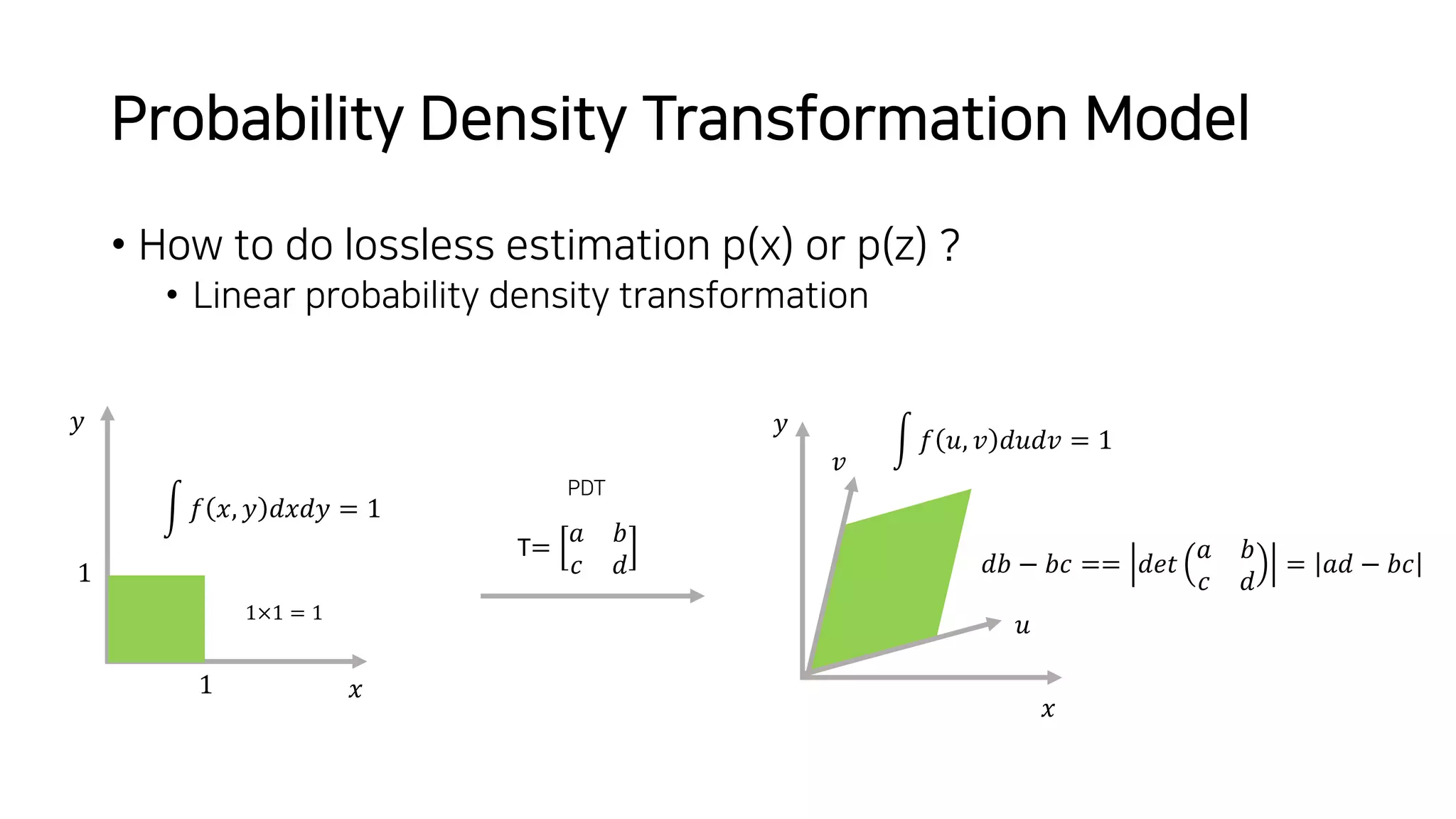
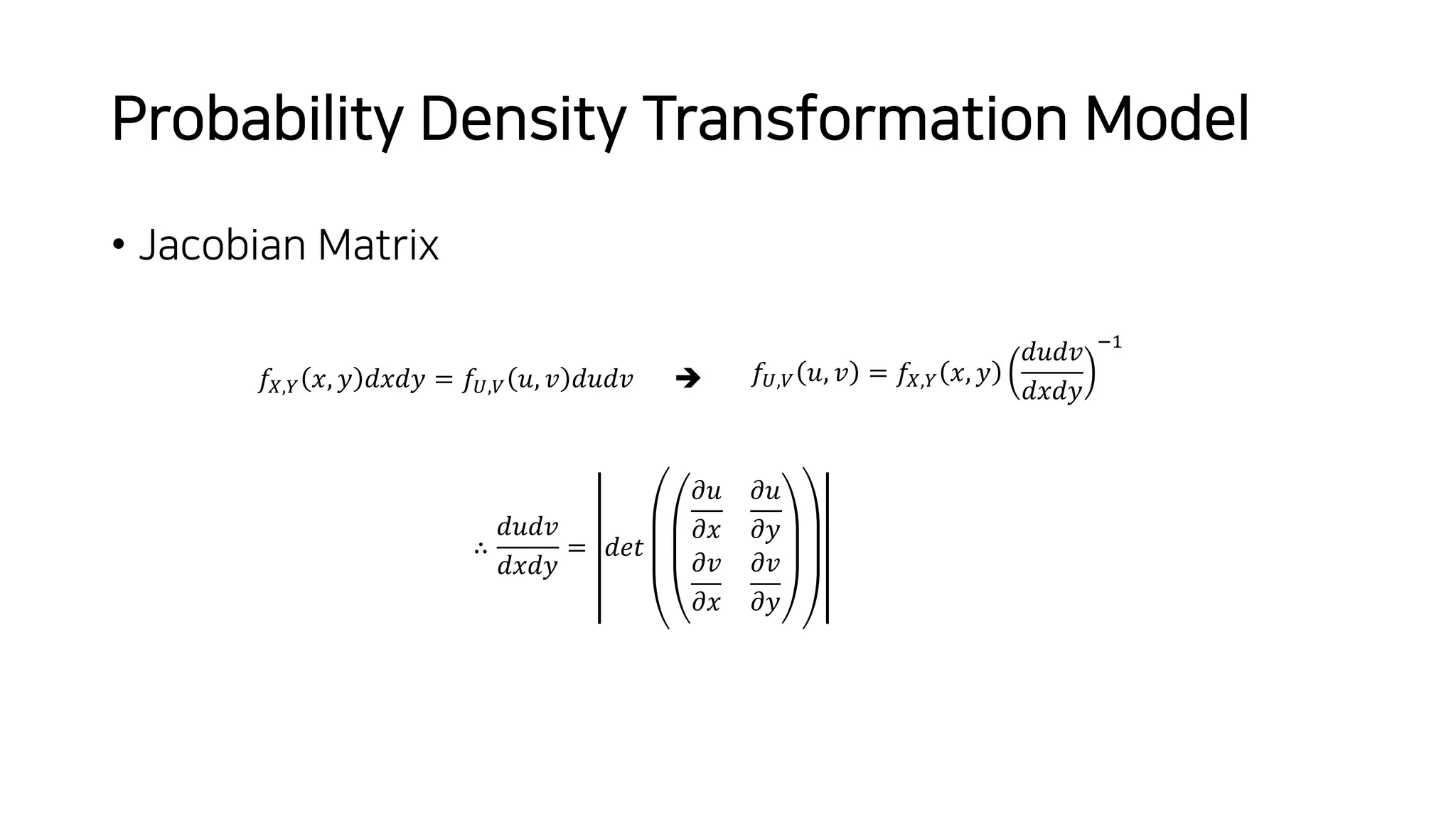
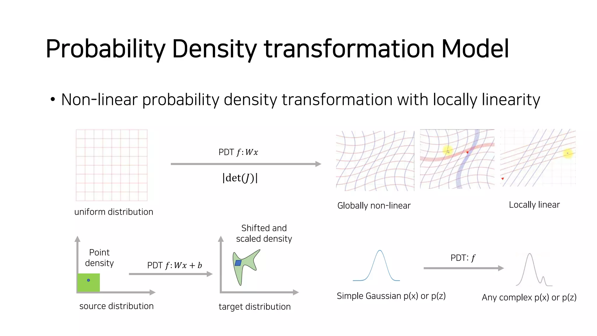
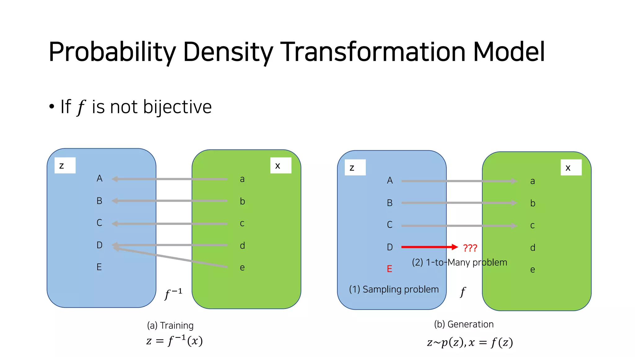
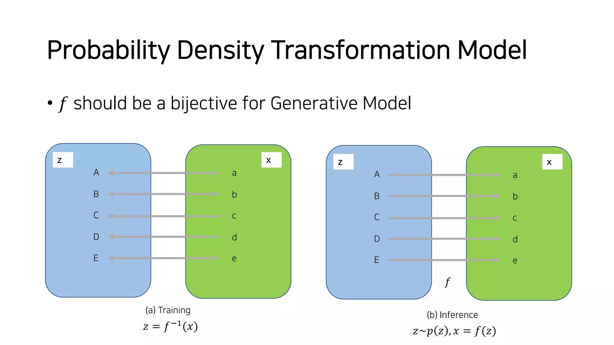
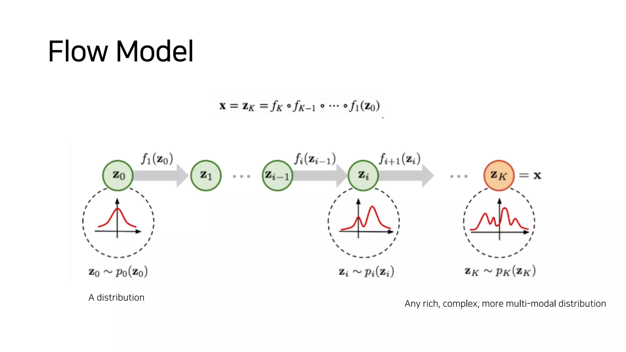
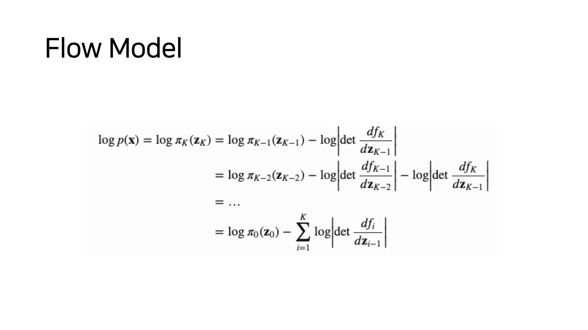
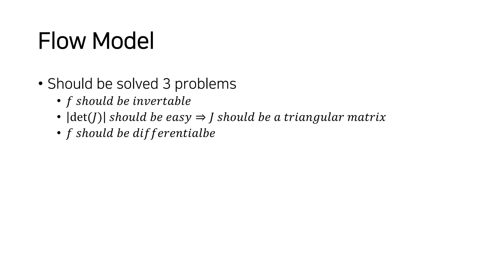
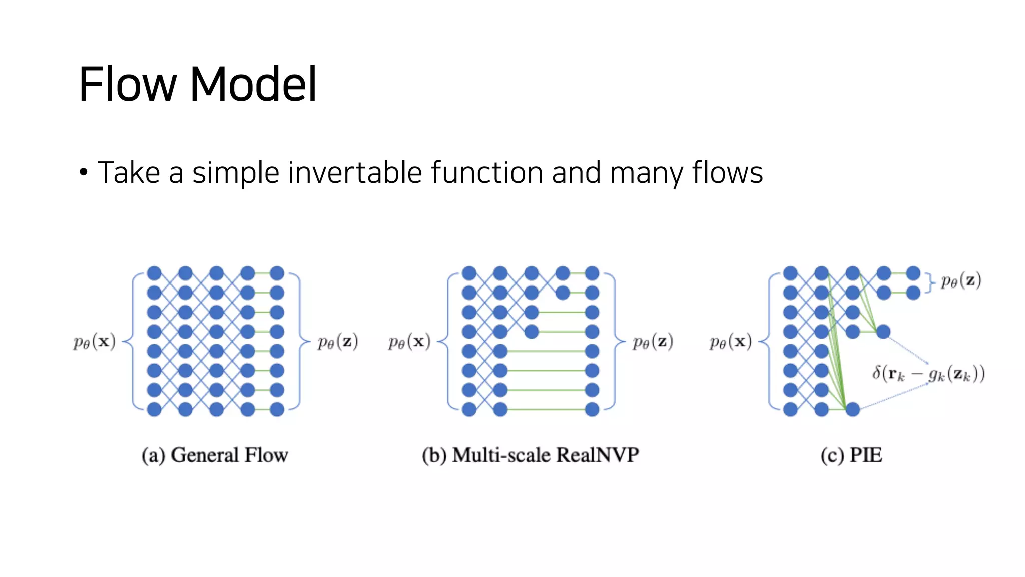
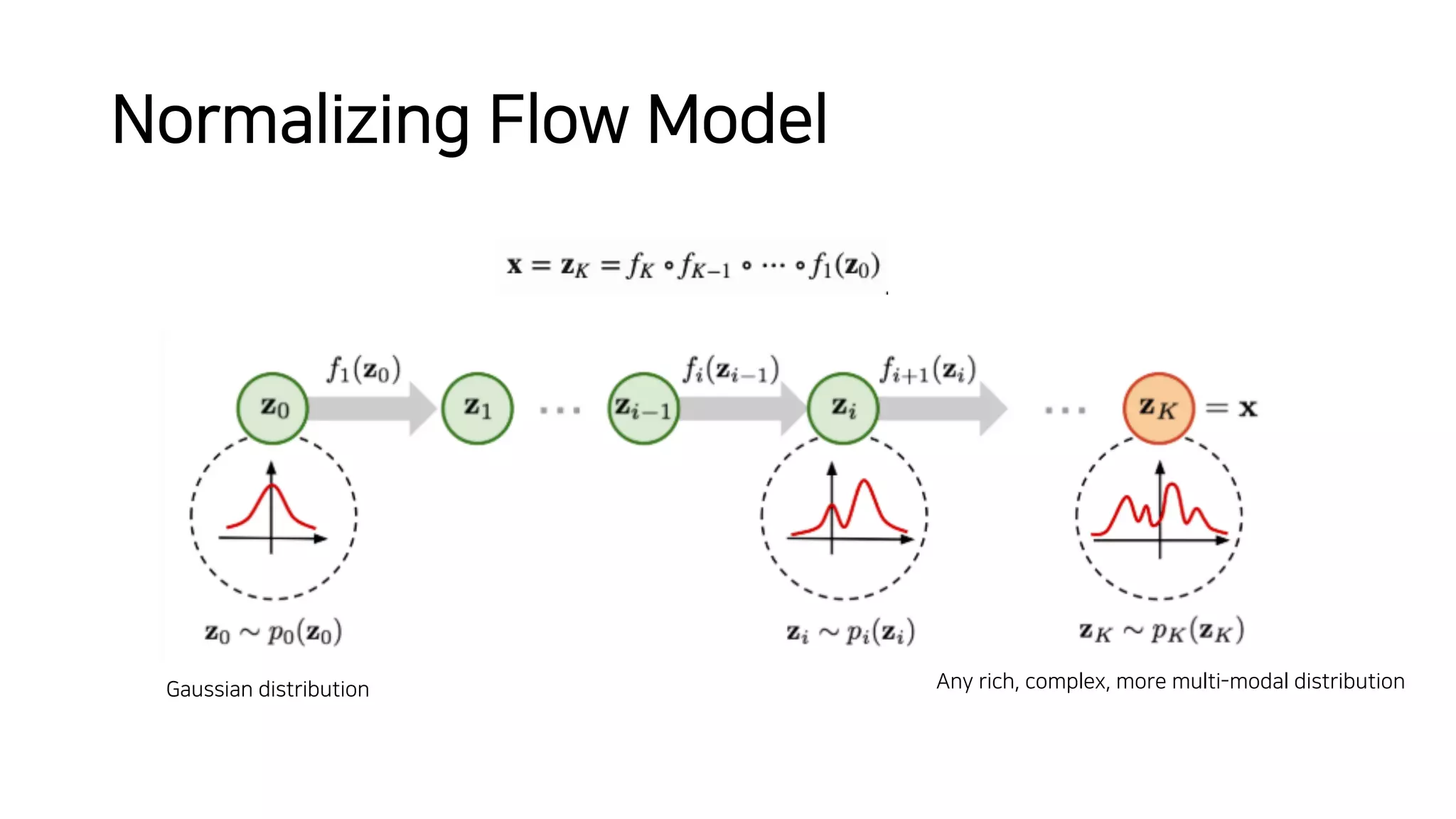
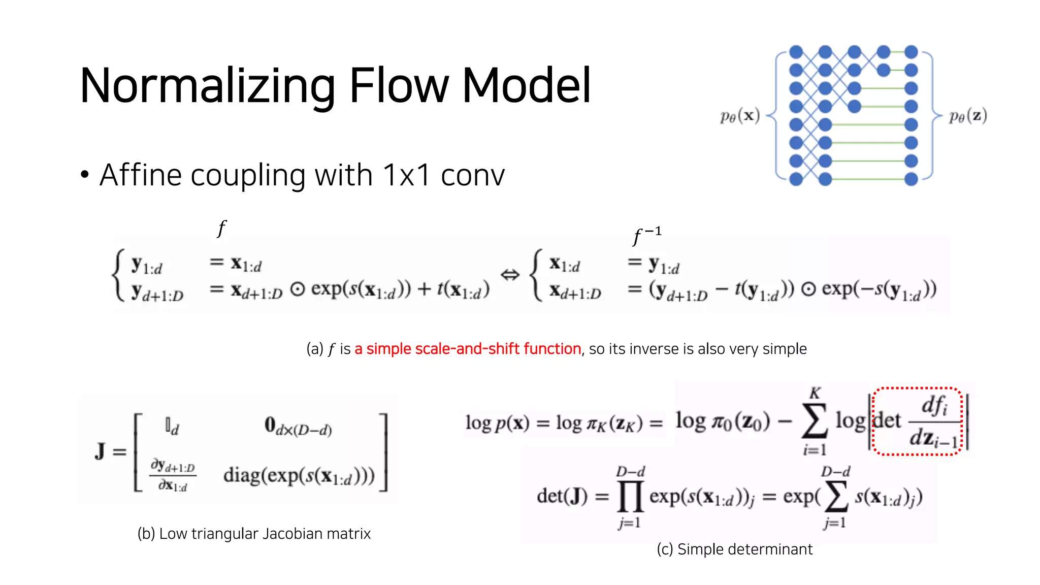
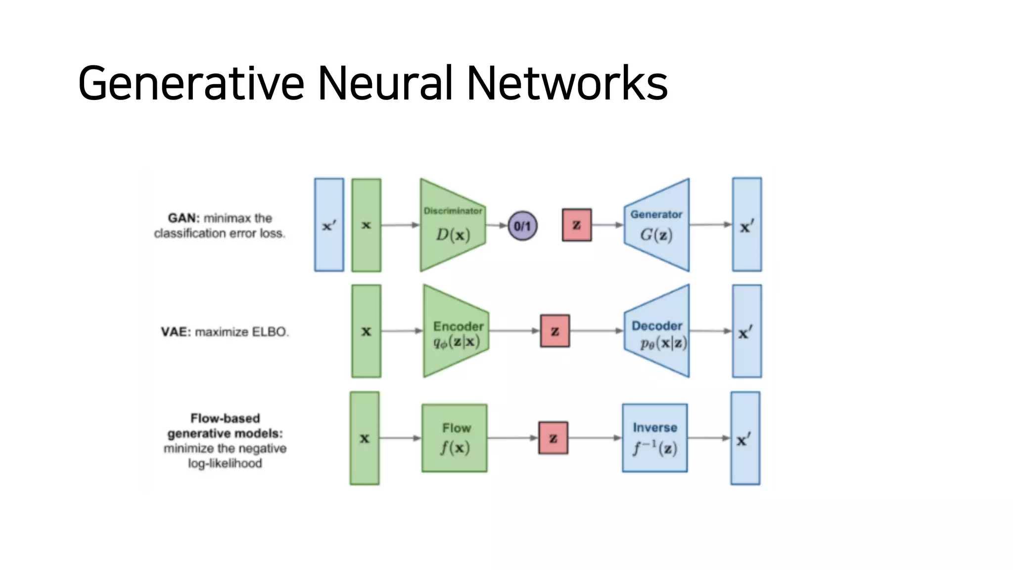
Normalizing flows can be used to transform a simple distribution like a Gaussian into a more complex target distribution through an invertible transformation. The transformation must be invertible to allow both generation and inference. It should also have an easily computable Jacobian determinant. Normalizing flow models achieve this by applying a series of simple invertible transformations with triangular Jacobians, such as affine coupling layers with 1x1 convolutions. This allows efficient and exact likelihood computation during both training and sampling from the modeled distribution.

1. Normalizing Flow
2020.06.24
kimjj.geek@gmail.com

2. Fully complete data
• Data
• Training
참고문헌: “기계학습”, 오일석

3. Generation & Classification
• Generation
• Classification
px = numpy.random.uniform(low=0.0, high=1.0)

4. Real world
• High dim., Spare, Small, Correlated, Missing, Corrupted, Hidden,…
20x20 è 400 dim vector
10ms
1024 wave samples è 1024 dim vector
or 80 dim melspectorgram vector

5. Real world
• Problems in terms of Generation
• Unstructed & Compex p(x), Sampling, Evaluation, …
𝑝!"#"(𝑥)𝑝(𝑥)
Hidden structures or latents
𝑝$%!&'(𝑥)

6. Latent variable Model
• x = True component + Noise component
𝑝!(𝑥)
𝑧
𝑥′
𝑥 = 𝑧 + 𝑒
Training
max
!
$
"
𝑙𝑜𝑔𝑝! 𝑥"
= $
"
𝑙𝑜𝑔 $
#
𝑝$(𝑧) 𝑝!(𝑥"
|𝑧)
Evaluation
𝑝! 𝑥 = $
#
𝑝$(𝑧)𝑝!(𝑥|𝑧)
Generation
𝑧 ~ 𝑝$(𝑧)
𝑥%~ 𝑝!(𝑥|𝑧)
𝑝"(𝑧)

7. Variational Inference Model
• If z is an impractical number of values or too complex
𝑧
𝑥′
𝑥 = 𝑧 + 𝑒𝑝!(𝑥)
Training
max
!
$
"
𝑙𝑜𝑔𝑝! 𝑥" = $
"
𝑙𝑜𝑔 $
#
𝑝$(𝑧) 𝑝!(𝑥" |𝑧)
𝑝! 𝑥 = ∫ 𝑝!(𝑧) 𝑝! 𝑥 𝑧 𝑑𝑧
intractable
Evaluation
𝑝! 𝑧 𝑥 = 𝑝!(𝑥|𝑧)𝑝!(𝑧)/𝑝!(𝑥)
intractable

8. Variational Inference Model
• Solution: Variational transformation
𝑧
𝑥′
𝑥 = 𝑧 + 𝑒
𝑝!∗(𝑧|𝑥) 𝑞∅∗(𝑧|𝑥)
𝐸𝑛𝑐𝑜𝑑𝑒𝑟
𝑞∅(𝑧|𝑥)
𝜇#|( ∑#|(
training
𝜇(|# ∑(|#
De𝑐𝑜𝑑𝑒𝑟
𝑝!(𝑥|𝑧)
Generation

9. Probability Density Transformation Model
• How to do lossless estimation p(x) or p(z) ?
• Linear probability density transformation
𝑥
𝑦
1
1
= 𝑓 𝑥, 𝑦 𝑑𝑥𝑑𝑦 = 1
T=
𝑎 𝑏
𝑐 𝑑
PDT
𝑣
𝑢
= 𝑓 𝑢, 𝑣 𝑑𝑢𝑑𝑣 = 1
1×1 = 1
𝑑𝑏 − 𝑏𝑐 == 𝑑𝑒𝑡
𝑎 𝑏
𝑐 𝑑
= 𝑎𝑑 − 𝑏𝑐
𝑦
𝑥

10. Probability Density Transformation Model
• Jacobian Matrix
𝑓),+ 𝑥, 𝑦 𝑑𝑥𝑑𝑦 = 𝑓,,- 𝑢, 𝑣 𝑑𝑢𝑑𝑣 è 𝑓,,- 𝑢, 𝑣 = 𝑓),+ 𝑥, 𝑦
𝑑𝑢𝑑𝑣
𝑑𝑥𝑑𝑦
./
∴
𝑑𝑢𝑑𝑣
𝑑𝑥𝑑𝑦
= 𝑑𝑒𝑡
𝜕𝑢
𝜕𝑥
𝜕𝑢
𝜕𝑦
𝜕𝑣
𝜕𝑥
𝜕𝑣
𝜕𝑦

11. Probability Density transformation Model
• Non-linear probability density transformation with locally linearity
source distribution
Point
density
target distribution
Globally non-linear Locally linear
uniform distribution
Simple Gaussian p(x) or p(z) Any complex p(x) or p(z)
PDT: 𝑓
PDT 𝑓: 𝑊𝑥 + 𝑏
Shifted and
scaled density
PDT 𝑓: 𝑊𝑥
det(𝐽)

12. Probability Density Transformation Model
• If 𝑓 is not bijective
A
B
C
D
E
a
b
c
d
e
z x
𝑓
(b) Generation
A
B
C
D
E
a
b
c
d
e
z x
𝑓./
(a) Training
???
𝑧 = 𝑓./
(𝑥) 𝑧~𝑝 𝑧 , 𝑥 = 𝑓(𝑧)
(2) 1-to-Many problem
(1) Sampling problem

13. Probability Density Transformation Model
• 𝑓 should be a bijective for Generative Model
A
B
C
D
E
a
b
c
d
e
z x
𝑓
(b) Inference
A
B
C
D
E
a
b
c
d
e
z x
𝑧 = 𝑓./(𝑥)
(a) Training
𝑧~𝑝 𝑧 , 𝑥 = 𝑓(𝑧)

14. Flow Model
A distribution
Any rich, complex, more multi-modal distribution

15. Flow Model

16. Flow Model
• Should be solved 3 problems
• 𝑓 𝑠ℎ𝑜𝑢𝑙𝑑 𝑏𝑒 𝑖𝑛𝑣𝑒𝑟𝑡𝑎𝑏𝑙𝑒
• det(𝐽) 𝑠ℎ𝑜𝑢𝑙𝑑 𝑏𝑒 𝑒𝑎𝑠𝑦 ⇒ 𝐽 𝑠ℎ𝑜𝑢𝑙𝑑 𝑏𝑒 𝑎 𝑡𝑟𝑖𝑎𝑛𝑔𝑢𝑙𝑎𝑟 𝑚𝑎𝑡𝑟𝑖𝑥
• 𝑓 𝑠ℎ𝑜𝑢𝑙𝑑 𝑏𝑒 𝑑𝑖𝑓𝑓𝑒𝑟𝑒𝑛𝑡𝑖𝑎𝑙𝑏𝑒

17. Flow Model
• Take a simple invertable function and many flows

18. Normalizing Flow Model
Gaussian distribution Any rich, complex, more multi-modal distribution

19. Normalizing Flow Model
• Affine coupling with 1x1 conv
𝑓 𝑓./
(a) 𝑓 is a simple scale-and-shift function, so its inverse is also very simple
(b) Low triangular Jacobian matrix
(c) Simple determinant

20. Flow Model

21. Generative Neural Networks