SlideShare a Scribd company logo
1 of 33
Download to read offline
29
2: Describing Data with Numerical Measures
2.1 a The dotplot shown below plots the five measurements along the horizontal axis. Since there are two
“1”s, the corresponding dots are placed one above the other. The approximate center of the data appears to
be around 1.
543210
Dotplot
median
mode
mean
b The mean is the sum of the measurements divided by the number of measurements, or
0 5 1 1 3 10
2
5 5
ix
x
n
∑ + + + +
= = = =
To calculate the median, the observations are first ranked from smallest to largest: 0, 1, 1, 3, 5. Then since
5n = , the position of the median is 0.5( 1) 3n + = , and the median is the 3rd
ranked measurement, or 1m = .
The mode is the measurement occurring most frequently, or mode = 1.
c The three measures in part b are located on the dotplot. Since the median and mode are to the left of
the mean, we conclude that the measurements are skewed to the right.
2.2 a The mean is
3 2 5 32
4
8 8
ix
x
n
∑ + + +
= = = =
b To calculate the median, the observations are first ranked from smallest to largest:
2, 3, 3, 4, 4, 5, 5, 6
Since 8n = is even, the position of the median is 0.5( 1) 4.5n + = , and the median is the average of the 4th
and 5th
measurements, or ( )4 4 2 4m = + = .
c Since the mean and the median are equal, we conclude that the measurements are symmetric. The
dotplot shown below confirms this conclusion.
65432
Dotplot
Introduction to Probability and Statistics 13th Edition Mendenhall Solutions Manual
Full Download: http://alibabadownload.com/product/introduction-to-probability-and-statistics-13th-edition-mendenhall-solutions-m
This sample only, Download all chapters at: alibabadownload.com
30
2.3 a
58
5.8
10
ix
x
n
∑
= = =
b The ranked observations are: 2, 3, 4, 5, 5, 6, 6, 8, 9, 10. Since 10n = , the median is halfway between
the 5th
and 6th
ordered observations, or ( )5 6 2 5.5m = + = .
c There are two measurements, 5 and 6, which both occur twice. Since this is the highest frequency of
occurrence for the data set, we say that the set is bimodal with modes at 5 and 6.
2.4 a
9455
2363.75
4
ix
x
n
∑
= = = b
8280
2070
4
ix
x
n
∑
= = =
c The average premium cost in several different cities is not as important to the consumer as the average
cost for a variety of consumers in his or her geographical area.
2.5 a Although there may be a few households who own more than one DVD player, the majority should
own either 0 or 1. The distribution should be slightly skewed to the right.
b Since most households will have only one DVD player, we guess that the mode is 1.
c The mean is
1 0 1 27
1.08
25 25
ix
x
n
∑ + + +
= = = =
To calculate the median, the observations are first ranked from smallest to largest: There are six 0s,
thirteen 1s, four 2s, and two 3s. Then since 25n = , the position of the median is 0.5( 1) 13n + = , which is
the 13th
ranked measurement, or 1m = . The mode is the measurement occurring most frequently, or
mode = 1.
d The relative frequency histogram is shown below, with the three measures superimposed. Notice that
the mean falls slightly to the right of the median and mode, indicating that the measurements are slightly
skewed to the right.
VCRs
Relativefrequency
3210
10/25
5/25
0
median
mode
mean
2.6 a The stem and leaf plot below was generated by Minitab. It is skewed to the right.
Stem-and-Leaf Display: Revenues
Stem-and-leaf of Revenues N = 10
Leaf Unit = 10000
2 0 33
(4) 0 5555
4 0
4 0 889
1 1
1 1
1 1
1 1
1 1 9
31
b The mean is
192604 91134 38416 736951
73,695.10
10 10
ix
x
n
∑ + + +
= = = =
To calculate the median, notice that the observations are already ranked from smallest to largest. Then
since 10n = , the position of the median is 0.5( 1) 5.5n + = , the average of the 5th
and 6th
ranked
measurements or ( )54848 52620 2 53,734m = + = .
c Since the mean is strongly affected by outliers, the median would be a better measure of center for
this data set.
2.7 It is obvious that any one family cannot have 2.5 children, since the number of children per family is a
quantitative discrete variable. The researcher is referring to the average number of children per family
calculated for all families in the United States during the 1930s. The average does not necessarily have to
be integer-valued.
2.8 a Similar to previous exercises. The mean is
0.99 1.92 0.66 12.55
0.896
14 14
ix
x
n
∑ + + +
= = = =
b To calculate the median, rank the observations from smallest to largest. The position of the median is
0.5( 1) 7.5n + = , and the median is the average of the 7th
and 8th
ranked measurement or
( )0.67 0.69 2 0.68m = + = .
c Since the mean is slightly larger than the median, the distribution is slightly skewed to the right.
2.9 The distribution of sports salaries will be skewed to the right, because of the very high salaries of some
sports figures. Hence, the median salary would be a better measure of center than the mean.
2.10 a Similar to previous exercises.
2150
215
10
ix
x
n
∑
= = =
b The ranked observations are shown below:
175 225
185 230
190 240
190 250
200 265
The position of the median is 0.5( 1) 5.5n + = and the median is the average of the 5th
and 6th
observation or
200 225
212.5
2
+
=
c Since there are no unusually large or small observations to affect the value of the mean, we would
probably report the mean or average time on task.
2.11 a Similar to previous exercises.
85
4.72
18
ix
x
n
∑
= = =
The ranked observations are:
1 1 3 6 12
1 1 4 7 16
1 2 4 7
1 2 5 11
The median is the average of the 9th
and 10th
observations or
32
m = (3 + 4)/2 = 3.5 and the mode is the most frequently occurring observation—mode = 1.
b Since the mean is larger than the median, the data are skewed to the right.
c The dotplot is shown below. The distribution is skewed to the right.
161412108642
Starbucks
Dotplot of Starbucks
2.12 a
19850
1985
10
ix
x
n
∑
= = =
b The ranked data are: 1200, 1300, 1350, 1500, 1800, 2000, 2200, 2600, 2900, 3000 and the median is
the average of the 5th
and 6th
observations or
1800 2000
1900
2
m
+
= =
c Average cost would not be as important as many other variables, such as picture quality, sound
quality, size, lowest cost for the best quality, and many other considerations.
2.13 a
12
2.4
5
ix
x
n
∑
= = =
b Create a table of differences, ( )ix x− and their squares, ( )
2
ix x− .
ix ix x− ( )
2
ix x−
2 –0.4 0.16
1 –1.4 1.96
1 –1.4 1.96
3 0.6 0.36
5 2.6 6.76
Total 0 11.20
Then
( )
2 2 2
2 (2 2.4) (5 2.4) 11.20
2.8
1 4 4
ix x
s
n
∑ − − + + −
= = = =
−
c The sample standard deviation is the positive square root of the variance or
2
2.8 1.673s s= = =
d Calculate 2 2 2 2
2 1 5 40ix∑ = + + + = . Then
( ) ( )
2 2
2
2
12
40
11.25 2.8
1 4 4
i
i
x
x
ns
n
∑
∑ − −
= = = =
−
and 2
2.8 1.673s s= = = .
The results of parts a and b are identical.
33
2.14 The results will vary from student to student, depending on their particular type of calculator. The results
should agree with Exercise 2.13.
2.15 a The range is 4 1 3R = − = . b
17
2.125
8
ix
x
n
∑
= = =
c Calculate 2 2 2 2
4 1 2 45ix∑ = + + + = . Then
( ) ( )
2 2
2
2
17
45
8.8758 1.2679
1 7 7
i
i
x
x
ns
n
∑
∑ − −
= = = =
−
and 2
1.2679 1.126s s= = = .
2.16 a The range is 6 1 5R = − = . b
31
3.875
8
ix
x
n
∑
= = =
c Calculate 2 2 2 2
3 1 5 137ix∑ = + + + = . Then
( ) ( )
2 2
2
2
31
137
16.8758 2.4107
1 7 7
i
i
x
x
ns
n
∑
∑ − −
= = = =
−
and 2
2.4107 1.55s s= = = .
d The range, 5R = , is 5 1.55 3.23= standard deviations.
2.17 a The range is 2.39 1.28 1.11R = − = .
b Calculate 2 2 2 2
1.28 2.39 1.51 15.415ix∑ = + + + = . Then
( ) ( )
2 2
2
2
8.56
15.415
.760285 .19007
1 4 4
i
i
x
x
ns
n
∑
∑ − −
= = = =
−
and 2
.19007 .436s s= = =
c The range, 1.11R = , is 1.11 .436 2.5= standard deviations.
2.18 a The range is 343.50 162.64 180.86R = − = . b
2940.2
245.02
12
ix
x
n
∑
= = =
c Calculate 2 2 2 2
266.63 163.41 230.46 763773.912ix∑ = + + + = . Then
( ) ( )
2 2
2
2
2940.2
763773.912
12 3943.264424
1 11
i
i
x
x
ns
n
∑
∑ − −
= = =
−
and 2
3943.264424 62.795s s= = = .
2.19 a The range of the data is 6 1 5R = − = and the range approximation with 10n = is
1.67
3
R
s ≈ =
b The standard deviation of the sample is
( ) ( )
2 2
2
2
32
130
10 3.0667 1.751
1 9
i
i
x
x
ns s
n
∑
∑ − −
= = = = =
−
which is very close to the estimate for part a.
c-e From the dotplot on the next page, you can see that the data set is not mound-shaped. Hence you can
use Tchebysheff’s Theorem, but not the Empirical Rule to describe the data.
34
654321
Dotplot
2.20 a First calculate the intervals:
36 3 or 33 to 39
2 36 6 or 30 to 42
3 36 9 or 27 to 45
x s
x s
x s
± = ±
± = ±
± = ±
According to the Empirical Rule, approximately 68% of the measurements will fall in the interval 33 to 39;
approximately 95% of the measurements will fall between 30 and 42; approximately 99.7% of the
measurements will fall between 27 and 45.
b If no prior information as to the shape of the distribution is available, we use Tchebysheff’s Theorem.
We would expect at least ( )2
1 1 1 0− = of the measurements to fall in the interval 33 to 39; at least
( )2
1 1 2 3 4− = of the measurements to fall in the interval 30 to 42; at least ( )2
1 1 3 8 9− = of the
measurements to fall in the interval 27 to 45.
2.21 a The interval from 40 to 60 represents 50 10μ σ± = ± . Since the distribution is relatively mound-
shaped, the proportion of measurements between 40 and 60 is 68% according to the Empirical Rule and is
shown below.
b Again, using the Empirical Rule, the interval 2 50 2(10)μ σ± = ± or between 30 and 70 contains
approximately 95% of the measurements.
35
c Refer to the figure below.
Since approximately 68% of the measurements are between 40 and 60, the symmetry of the distribution
implies that 34% of the measurements are between 50 and 60. Similarly, since 95% of the measurements
are between 30 and 70, approximately 47.5% are between 30 and 50. Thus, the proportion of
measurements between 30 and 60 is
0.34 0.475 0.815+ =
d From the figure in part a, the proportion of the measurements between 50 and 60 is 0.34 and the
proportion of the measurements which are greater than 50 is 0.50. Therefore, the proportion that are
greater than 60 must be
0.5 0.34 0.16− =
2.22 Since nothing is known about the shape of the data distribution, you must use Tchebysheff’s Theorem to
describe the data.
a The interval from 60 to 90 represents 3μ σ± which will contain at least 8/9 of the measurements.
b The interval from 65 to 85 represents 2μ σ± which will contain at least 3/4 of the measurements.
c The value 65x = lies two standard deviations below the mean. Since at least 3/4 of the measurements
are within two standard deviation range, at most 1/4 can lie outside this range, which means that at most 1/4
can be less than 65.
2.23 a The range of the data is 1.1 0.5 0.6R = − = and the approximate value of s is
0.2
3
R
s ≈ =
b Calculate 7.6ix∑ = and 2
6.02ix∑ = , the sample mean is
7.6
.76
10
ix
x
n
∑
= = =
and the standard deviation of the sample is
( ) ( )
2 2
2
2
7.6
6.02
0.24410 0.165
1 9 9
i
i
x
x
ns s
n
∑
∑ − −
= = = = =
−
which is very close to the estimate from part a.
36
2.24 a The stem and leaf plot generated by Minitab shows that the data is roughly mound-shaped. Note
however the gap in the center of the distribution and the two measurements in the upper tail.
Stem-and-Leaf Display: Weight
Stem-and-leaf of Weight N = 27
Leaf Unit = 0.010
1 7 5
2 8 3
6 8 7999
8 9 23
13 9 66789
13 10
(3) 10 688
11 11 2244
7 11 788
4 12 4
3 12 8
2 13
2 13 8
1 14 1
b Calculate 28.41ix∑ = and 2
30.6071ix∑ = , the sample mean is
28.41
1.052
27
ix
x
n
∑
= = =
and the standard deviation of the sample is
( ) ( )
2 2
2
2
28.41
30.6071
27 0.166
1 26
i
i
x
x
ns s
n
∑
∑ − −
= = = =
−
c The following table gives the actual percentage of measurements falling in the intervals x ks± for
1,2,3k = .
k x ks± Interval Number in Interval Percentage
1 1.052 0.166± 0.866 to 1.218 21 78%
2 1.052 0.332± 0.720 to 1.384 26 96%
3 1.052 0.498± 0.554 to 1.550 27 100%
d The percentages in part c do not agree too closely with those given by the Empirical Rule, especially
in the one standard deviation range. This is caused by the lack of mounding (indicated by the gap) in the
center of the distribution.
e The lack of any one-pound packages is probably a marketing technique intentionally used by the
supermarket. People who buy slightly less than one-pound would be drawn by the slightly lower price,
while those who need exactly one-pound of meat for their recipe might tend to opt for the larger package,
increasing the store’s profit.
2.25 According to the Empirical Rule, if a distribution of measurements is approximately mound-shaped,
a approximately 68% or 0.68 of the measurements fall in the interval 12 2.3 or 9.7 to 14.3μ σ± = ±
b approximately 95% or 0.95 of the measurements fall in the interval 2 12 4.6 or 7.4 to 16.6μ σ± = ±
c approximately 99.7% or 0.997 of the measurements fall in the interval 3 12 6.9 or 5.1 to 18.9μ σ± = ±
Therefore, approximately 0.3% or 0.003 will fall outside this interval.
37
2.26 a The stem and leaf plots are shown below. The second set has a slightly higher location and spread.
Stem-and-Leaf Display: Method 1, Method 2
Stem-and-leaf of Method 1 N = 10 Stem-and-leaf of Method 2 N = 10
Leaf Unit = 0.00010 Leaf Unit = 0.00010
1 10 0
3 11 00 1 11 0
4 12 0 3 12 00
(4) 13 0000 5 13 00
2 14 0 5 14 0
1 15 0 4 15 00
2 16 0
1 17 0
b Method 1: Calculate 0.125ix∑ = and 2
0.001583ix∑ = . Then 0.0125ix
x
n
∑
= = and
( ) ( )
2 2
2
2
0.125
0.001583
10 0.00151
1 9
i
i
x
x
ns s
n
∑
∑ − −
= = = =
−
Method 2: Calculate 0.138ix∑ = and 2
0.001938ix∑ = . Then 0.0138ix
x
n
∑
= = and
( ) ( )
2 2
2
2
0.138
0.001938
10 0.00193
1 9
i
i
x
x
ns s
n
∑
∑ − −
= = = =
−
The results confirm the conclusions of part a.
2.27 a The center of the distribution should be approximately halfway between 0 and 9 or ( )0 9 2 4.5+ = .
b The range of the data is 9 0 9R = − = . Using the range approximation, 4 9 4 2.25s R≈ = = .
c Using the data entry method the students should find 4.586x = and 2.892s = , which are fairly close
to our approximations.
2.28 a Similar to previous exercises. The intervals, counts and percentages are shown in the table.
k x ks± Interval Number in Interval Percentage
1 4.586 2.892± 1.694 to 7.478 43 61%
2 4.586 5.784± –1.198 to 10.370 70 100%
3 4.586 8.676± –4.090 to 13.262 70 100%
b The percentages in part a do not agree with those given by the Empirical Rule. This is because the
shape of the distribution is not mound-shaped, but flat.
2.29 a Although most of the animals will die at around 32 days, there may be a few animals that survive a
very long time, even with the infection. The distribution will probably be skewed right.
b Using Tchebysheff’s Theorem, at least 3/4 of the measurements should be in the interval
32 72μ σ± ⇒ ± or 0 to 104 days.
2.30 a The value of x is 32 36 4μ σ− = − = − .
b The interval is 32 36μ σ± ± should contain approximately ( )100 68 34%− = of the survival times, of
which 17% will be longer than 68 days and 17% less than –4 days.
c The latter is clearly impossible. Therefore, the approximate values given by the Empirical Rule are
not accurate, indicating that the distribution cannot be mound-shaped.
38
2.31 a We choose to use 12 classes of length 1.0. The tally and the relative frequency histogram follow.
Class i Class Boundaries Tally fi Relative frequency, fi/n
1 2 to < 3 1 1 1/70
2 3 to < 4 1 1 1/70
3 4 to < 5 111 3 3/70
4 5 to < 6 11111 5 5/70
5 6 to < 7 11111 5 5/70
6 7 to < 8 11111 11111 11 12 12/70
7 8 to < 9 11111 11111 11111 111 18 18/70
8 9 to < 10 11111 11111 11111 15 15/70
9 10 to < 11 11111 1 6 6/70
10 11 to < 12 111 3 3/70
11 12 to < 13 0 0
12 13 to < 14 1 1 1/70
TREES
Relativefrequency
15105
20/70
10/70
0
b Calculate 70, 541in x= ∑ = and 2
4453ix∑ = . Then
541
7.729
70
ix
x
n
∑
= = = is an estimate of μ .
c The sample standard deviation is
( ) ( )
2 2
2 541
4453
70 3.9398 1.985
1 69
i
i
x
x
ns
n
∑
∑ − −
= = = =
−
The three intervals, x ks± for 1,2,3k = are calculated below. The table shows the actual percentage of
measurements falling in a particular interval as well as the percentage predicted by Tchebysheff’s Theorem
and the Empirical Rule. Note that the Empirical Rule should be fairly accurate, as indicated by the mound-
shape of the histogram in part a.
k x ks± Interval Fraction in Interval Tchebysheff Empirical Rule
1 7.729 1.985± 5.744 to 9.714 50/70 = 0.71 at least 0 0.68≈
2 7.729 3.970± 3.759 to 11.699 67/70 = 0.96 at least 0.75 0.95≈
3 7.729 5.955± 1.774 to 13.684 70/70 = 1.00 at least 0.89 0.997≈
2.32 a Calculate 1.92 0.53 1.39R = − = so that 4 1.39 4 0.3475s R≈ = = .
b Calculate 14, 12.55in x= ∑ = and 2
13.3253ix∑ = . Then
( ) ( )
2 2
2
2
12.55
13.3253
14 0.1596
1 13
i
i
x
x
ns
n
∑
∑ − −
= = =
−
and 0.15962 0.3995s = =
which is fairly close to the approximate value of s from part a.
39
2.33 a-b Calculate 93 51 42R = − = so that 4 42 4 10.5s R≈ = = .
c Calculate 30, 2145in x= ∑ = and 2
158,345ix∑ = . Then
( ) ( )
2 2
2
2
2145
158,345
30 171.6379
1 29
i
i
x
x
ns
n
∑
∑ − −
= = =
−
and 171.6379 13.101s = =
which is fairly close to the approximate value of s from part b.
d The two intervals are calculated below. The proportions agree with Tchebysheff’s Theorem, but are
not to close to the percentages given by the Empirical Rule. (This is because the distribution is not quite
mound-shaped.)
k x ks± Interval Fraction in Interval Tchebysheff Empirical Rule
2 71.5 26.20± 45.3 to 97.7 30/30 = 1.00 at least 0.75 0.95≈
3 71.5 39.30± 32.2 to 110.80 30/30 = 1.00 at least 0.89 0.997≈
2.34 a Answers will vary. A typical histogram is shown below. The distribution is skewed to the right.
1612840
.35
.30
.25
.20
.15
.10
.05
0
Kids
Relativefrequency
b Calculate 42, 151in x= ∑ = and 2
897ix∑ = . Then
( ) ( )
2 2
2
2
151
3.60,
42
151
897
42 8.63705
1 41
i
i
i
x
x
n
x
x
ns
n
∑
= = =
∑
∑ − −
= = =
−
and 8.63705 2.94s = =
c The three intervals, x ks± for 1,2,3k = are calculated below. The table shows the actual percentage
of measurements falling in a particular interval as well as the percentage predicted by Tchebysheff’s
Theorem and the Empirical Rule. Note that the Empirical Rule is not very accurate for the first interval,
since the histogram in part a is skewed.
k x ks± Interval Fraction in Interval Tchebysheff Empirical Rule
1 3.60 2.94± .66 to 6.54 32/42 = .76 at least 0 0.68≈
2 3.60 5.88± −2.28 to 9.48 40/42 = .95 at least 0.75 0.95≈
3 3.60 8.82± −5.22 to 12.42 41/42 = .976 at least 0.89 0.997≈
2.35 a Calculate 2.39 1.28 1.11R = − = so that 2.5 1.11 2.5 .444s R≈ = = .
b In Exercise 2.17, we calculated 8.56ix∑ = and 2 2 2 2
1.28 2.39 1.51 15.415ix∑ = + + + = . Then
( ) ( )
2 2
2
2
8.56
15.451
.760285 .19007
1 4 4
i
i
x
x
ns
n
∑
∑ − −
= = = =
−
40
and 2
.19007 .436s s= = = , which is very close to our estimate in part a.
2.36 a Answers will vary. A typical stem and leaf plot is generated by Minitab.
Stem-and-Leaf Display: Favre
Stem-and-leaf of Favre N = 16
Leaf Unit = 1.0
1 0 5
1 1
4 1 579
(8) 2 01222244
4 2 568
1 3 1
b Calculate 16, 343in x= ∑ = and 2
7875ix∑ = . Then
343
21.44
16
ix
x
n
∑
= = = ,
( ) ( )
2 2
2
2
343
7875
16 34.79583
1 15
i
i
x
x
ns
n
∑
∑ − −
= = =
−
and 2
34.795833 5.90s s= = = .
c Calculate 2 21.44 11.80 or 9.64 to 33.24.x s± ⇒ ± From the original data set, 15 of the 16
measurements, or about 94% fall in this interval.
2.37 a Calculate 15, 21in x= ∑ = and 2
49ix∑ = . Then
21
1.4
15
ix
x
n
∑
= = = and
( ) ( )
2 2
2
2
21
49
15 1.4
1 14
i
i
x
x
ns
n
∑
∑ − −
= = =
−
b Using the frequency table and the grouped formulas, calculate
0(4) 1(5) 2(2) 3(4) 21i ix f∑ = + + + =
2 2 2 2 2
0 (4) 1 (5) 2 (2) 3 (4) 49i ix f∑ = + + + =
Then, as in part a,
21
1.4
15
i ix f
x
n
∑
= = =
( ) ( )
2 2
2
2
21
49
15 1.4
1 14
i i
i i
x f
x f
ns
n
∑
∑ − −
= = =
−
2.38 Use the formulas for grouped data given in Exercise 2.37. Calculate 17, 79i in x f= ∑ = , and 2
393i ix f∑ = .
Then,
79
4.65
17
i ix f
x
n
∑
= = =
( ) ( )
2 2
2
2
79
393
17 1.6176
1 16
i i
i i
x f
x f
ns
n
∑
∑ − −
= = =
−
and 1.6176 1.27s = =
2.39 a The data in this exercise have been arranged in a frequency table.
xi 0 1 2 3 4 5 6 7 8 9 10
fi 10 5 3 2 1 1 1 0 0 1 1
Using the frequency table and the grouped formulas, calculate
0(10) 1(5) 10(1) 51i ix f∑ = + + + =
41
2 2 2 2
0 (10) 1 (5) 10 (1) 293i ix f∑ = + + + =
Then
51
2.04
25
i ix f
x
n
∑
= = =
( ) ( )
2 2
2
2
51
293
25 7.873
1 24
i i
i i
x f
x f
ns
n
∑
∑ − −
= = =
−
and 7.873 2.806s = = .
b-c The three intervals x ks± for 1,2,3k = are calculated in the table along with the actual proportion of
measurements falling in the intervals. Tchebysheff’s Theorem is satisfied and the approximation given by
the Empirical Rule are fairly close for 2k = and 3k = .
k x ks± Interval Fraction in Interval Tchebysheff Empirical Rule
1 2.04 2.806± –0.766 to 4.846 21/25 = 0.84 at least 0 0.68≈
2 2.04 5.612± –3.572 to 7.652 23/25 = 0.92 at least 0.75 0.95≈
3 2.04 8.418± –6.378 to 10.458 25/25 = 1.00 at least 0.89 0.997≈
2.40 The sorted data set, along with the positions of the quartiles and the quartiles themselves are shown in the
table.
Sorted Data Set n Position of Q1 Position of Q3 Lower quartile, Q1 Upper quartile, Q3
.13, 16, .21, .28, .34, .76, .88 7 .25(8) = 2 .75(8) = 6 .16 .76
1.0, 1.7, 2.0, 2.1, 2.3, 2.8,
2.9, 4.4, 5.1, 6.5, 8.8
11 .25(12) = 3 .75(12) = 9 2.0 5.1
2.41 The data have already been sorted. Find the positions of the quartiles, and the measurements that are just
above and below those positions. Then find the quartiles by interpolation.
Sorted Data Set Position of
Q1
Above
and below
Q1 Position of Q3 Above
and below
Q3
1, 1.5, 2, 2, 2.2 .25(6) = 1.5 1 and 1.5 1.25 .75(6) = 4.5 2 and 2.2 2.1
0, 1.7, 1.8, 3.1,
3.2, 7, 8, 8.8, 8.9,
9, 10
.25(12) = 3 None 1.8 .75(12) = 9 None 8.9
.23, .30, .35, .41,
.56, .58, .76, .80
.25(9) = 2.25 .30 and .35 .30 + .25(.05)
= .3125
.75(9) = 6.75 .58 and
.76
.58 +
.75(.18) =
.7150
2.42 The ordered data are:
0, 1, 3, 4, 4, 5, 6, 6, 7, 7, 8
a With 12n = , the median is in position 0.5( 1) 6.5n + = , or halfway between the 6th
and 7th
observations. The lower quartile is in position 0.25( 1) 3.25n + = (one-fourth of the way between the 3rd
and 4th
observations) and the upper quartile is in position 0.75( 1) 9.75n + = (three-fourths of the way
between the 9th
and 10th
observations). Hence, ( ) 15 6 2 5.5, 3 0.25(4 3) 3.25m Q= + = = + − = and
3 6 0.75(7 6) 6.75Q = + − = . Then the five-number summary is
Min Q1 Median Q3 Max
0 3.25 5.5 6.75 8
and
42
3 1 6.75 3.25 3.50IQR Q Q= − = − =
b Calculate 12, 57in x= ∑ = and 2
337ix∑ = . Then
57
4.75
12
ix
x
n
∑
= = = and the sample standard
deviation is
( ) ( )
2 2
2 57
337
12 6.022727 2.454
1 11
i
i
x
x
ns
n
∑
∑ − −
= = = =
−
c For the smaller observation, 0x = ,
0 4.75
-score 1.94
2.454
x x
z
s
− −
= = = −
and for the largest observation, 8x = ,
8 4.75
-score 1.32
2.454
x x
z
s
− −
= = =
Since neither z-score exceeds 2 in absolute value, none of the observations are unusually small or large.
2.43 The ordered data are:
0, 1, 5, 6, 7, 8, 9, 10, 12, 12, 13, 14, 16, 19, 19
With 15n = , the median is in position 0.5( 1) 8n + = , so that 10m = . The lower quartile is in position
0.25( 1) 4n + = so that 1 6Q = and the upper quartile is in position 0.75( 1) 12n + = so that 3 14Q = . Then
the five-number summary is
Min Q1 Median Q3 Max
0 6 10 14 19
and 3 1 14 6 8IQR Q Q= − = − = .
2.44 The ordered data are:
12, 18, 22, 23, 24, 25, 25, 26, 26, 27, 28
For 11n = , the position of the median is 0.5( 1) 0.5(11 1) 6n + = + = and 25m = . The positions of the
quartiles are 0.25( 1) 3n + = and 0.75( 1) 9n + = , so that 1 322, 26,Q Q= = and 26 22 4IQR = − = .
The lower and upper fences are:
1
3
1.5 22 6 16
1.5 26 6 32
Q IQR
Q IQR
− = − =
+ = + =
The only observation falling outside the fences is 12x = which is identified as an outlier. The box plot is
shown below. The lower whisker connects the box to the smallest value that is not an outlier, 18x = . The
upper whisker connects the box to the largest value that is not an outlier or 28x = .
x
3025201510
43
2.45 The ordered data are:
2, 3, 4, 5, 6, 6, 6, 7, 8, 9, 9, 10, 22
For 13n = , the position of the median is 0.5( 1) 0.5(13 1) 7n + = + = and 6m = . The positions of the
quartiles are 0.25( 1) 3.5n + = and 0.75( 1) 10.5n + = , so that 1 34.5, 9,Q Q= = and 9 4.5 4.5IQR = − = .
The lower and upper fences are:
1
3
1.5 4.5 6.75 2.25
1.5 9 6.75 15.75
Q IQR
Q IQR
− = − = −
+ = + =
The value 22x = lies outside the upper fence and is an outlier. The box plot is shown below. The lower
whisker connects the box to the smallest value that is not an outlier, which happens to be the minimum
value, 2x = . The upper whisker connects the box to the largest value that is not an outlier or 10x = .
x
2520151050
2.46 From Section 2.6, the 69th
percentile implies that 69% of all students scored below your score, and only
31% scored higher.
2.47 a The ordered data are shown below:
1.70 101.00 209.00 264.00 316.00 445.00
1.72 118.00 218.00 278.00 318.00 481.00
5.90 168.00 221.00 286.00 329.00 485.00
8.80 180.00 241.00 314.00 397.00
85.40 183.00 252.00 315.00 406.00
For 28n = , the position of the median is 0.5( 1) 14.5n + = and the positions of the quartiles are
0.25( 1) 7.25n + = and 0.75( 1) 21.75n + = . The lower quartile is ¼ the way between the 7th
and 8th
measurements or 1 118 0.25(168 118) 130.5Q = + − = and the upper quartile is ¾ the way between the 21st
and 22nd
measurements or 3 316 0.75(318 316) 317.5Q = + − = . Then the five-number summary is
Min Q1 Median Q3 Max
1.70 130.5 246.5 317.5 485
b Calculate 3 1 317.5 130.5 187IQR Q Q= − = − = . Then the lower and upper fences are:
1
3
1.5 130.5 280.5 150
1.5 317.5 280.5 598
Q IQR
Q IQR
− = − = −
+ = + =
44
The box plot is shown below. Since there are no outliers, the whiskers connect the box to the minimum
and maximum values in the ordered set.
Mercury
5004003002001000
c-d The boxplot does not identify any of the measurements as outliers, mainly because the large variation
in the measurements cause the IQR to be large. However, the student should notice the extreme difference
in the magnitude of the first four observations taken on young dolphins. These animals have not been alive
long enough to accumulate a large amount of mercury in their bodies.
2.48 a See Exercise 2.24b.
b For 1.38x = ,
1.38 1.05
-score 1.94
0.17
x x
z
s
− −
= = =
while for 1.41x = ,
1.41 1.05
-score 2.12
0.17
x x
z
s
− −
= = =
The value 1.41x = would be considered somewhat unusual, since its z-score exceeds 2 in absolute value.
c For 27n = , the position of the median is 0.5( 1) 0.5(27 1) 14n + = + = and 1.06m = . The positions of
the quartiles are 0.25( 1) 7n + = and 0.75( 1) 21n + = , so that 1 30.92, 1.17,Q Q= = and
1.17 0.92 0.25IQR = − = .
The lower and upper fences are:
1
3
1.5 0.92 0.375 0.545
1.5 1.17 0.375 1.545
Q IQR
Q IQR
− = − =
+ = + =
The box plot is shown below. Since there are no outliers, the whiskers connect the box to the minimum
and maximum values in the ordered set.
Weight
1.41.31.21.11.00.90.80.7
45
Since the median line is almost in the center of the box, the whiskers are nearly the same lengths, the data
set is relatively symmetric.
2.49 a For 16n = , the position of the median is 0.5( 1) 8.5n + = and the positions of the quartiles are
0.25( 1) 4.25n + = and 0.75( 1) 12.75n + = . The lower quartile is ¼ the way between the 4th
and 5th
measurements and the upper quartile is ¾ the way between the 12th
and 13th
measurements. The sorted
measurements are shown below.
Favre: 5, 15, 17, 19, 20, 21, 22, 22, 22, 22, 24, 24, 25, 26, 28, 31
Peyton Manning: 14, 14, 20, 20, 21, 21, 21, 22, 25, 25, 25, 26, 27, 29, 30, 32
For Brett Favre,
( )22 22 2 22m = + = , 1 19 0.25(20 19) 19.25Q = + − = and 3 24 0.75(25 24) 24.75Q = + − = .
For Peyton Manning,
( )22 25 2 23.50m = + = , 1 20 0.25(21 20) 20.25Q = + − = and 3 26 0.75(27 26) 26.75Q = + − = .
Then the five-number summaries are
Min Q1 Median Q3 Max
Favre 5 19.25 22 24.75 31
Manning 14 20.25 23.5 26.75 32
b For Brett Favre, calculate 3 1 24.75 19.25 5.5IQR Q Q= − = − = . Then the lower and upper fences are:
1
3
1.5 19.25 8.25 11
1.5 24.75 8.25 33
Q IQR
Q IQR
− = − =
+ = + =
and x = 5 is an outlier.
For Peyton Manning, calculate 3 1 26.75 20.25 6.5IQR Q Q= − = − = . Then the lower and upper fences are:
1
3
1.5 20.25 9.75 10.5
1.5 26.75 9.75 36.5
Q IQR
Q IQR
− = − =
+ = + =
and there are no outliers. The box plots are shown below.
Manning
Favre
3530252015105
Completed Passes
c Answers will vary. The Favre distribution is relatively symmetric except for the one outlier; the
Manning distribution is roughly symmetric, probably mound-shaped. The Manning distribution is slightly
more variable; Manning has a higher median number of completed passes.
2.50 Answers will vary from student to student. The distribution is skewed to the right with three outliers
(Truman, Cleveland and F. Roosevelt). The box plot is shown on the next page.
46
4003002001000
Vetoes
2.51 a Just by scanning through the 20 measurements, it seems that there are a few unusually small
measurements, which would indicate a distribution that is skewed to the left.
b The position of the median is 0.5( 1) 0.5(25 1) 10.5n + = + = and (120 127) / 2 123.5m = + = . The mean
is
2163
108.15
20
ix
x
n
∑
= = =
which is smaller than the median, indicate a distribution skewed to the left.
c The positions of the quartiles are 0.25( 1) 5.25n + = and 0.75( 1) 15.75n + = , so that
1 365 .25(87 65) 70.5, 144 .75(147 144) 146.25,Q Q= − − = = + − = and 146.25 70.5 75.75IQR = − = .
The lower and upper fences are:
1
3
1.5 70.5 113.625 43.125
1.5 146.25 113.625 259.875
Q IQR
Q IQR
− = − = −
+ = + =
The box plot is shown below. There are no outliers. The long left whisker and the median line located to
the right of the center of the box indicates that the distribution that is skewed to the left.
180160140120100806040200
Survival time
2.52 a The sorted data is:
162.64, 163.41, 187.16, 208.99, 219.41, 226.80
230.46, 266.63, 289.17, 306.55, 335.48, 343.50
47
The positions of the median and the quartiles are 0.5( 1) 6.5n + = , 0.25( 1) 3.25n + = and 0.75( 1) 9.75n + = ,
so that 1
3
(226.80 230.46) / 2 228.63
187.16 .25(208.99 187.16) 192.6175
289.17 .75(306.55 289.17) 302.205
m
Q
Q
= + =
= + − =
= + − =
and 302.205 192.6175 109.5875IQR = − = .
The lower and upper fences are:
1
3
1.5 192.6175 164.38125 28.236
1.5 302.205 164.38125 466.586
Q IQR
Q IQR
− = − =
+ = + =
There are no outliers, and the box plot is shown below.
350300250200150
Utility Bill
b Because of the slightly longer right whisker and the median line to the left of center, the distribution is
slightly skewed to the right.
2.53 Answers will vary. The student should notice the outliers in the female group, and that the median female
temperature is higher than the median male temperature.
2.54 a Calculate 14, 367in x= ∑ = and 2
9641ix∑ = . Then
367
26.214
14
ix
x
n
∑
= = = and
( ) ( )
2 2
2 367
9641
14 1.251
1 13
i
i
x
x
ns
n
∑
∑ − −
= = =
−
b Calculate 14, 366in x= ∑ = and 2
9644ix∑ = . Then
366
26.143
14
ix
x
n
∑
= = = and
( ) ( )
2 2
2 366
9644
14 2.413
1 13
i
i
x
x
ns
n
∑
∑ − −
= = =
−
c The centers are roughly the same; the Sunmaid raisins appear slightly more variable.
2.55 a The ordered sets are shown below:
Generic Sunmaid
24 25 25 25 26 22 24 24 24 24
26 26 26 26 27 25 25 27 28 28
27 28 28 28 28 28 29 30
For 14n = , the position of the median is 0.5( 1) 0.5(14 1) 7.5n + = + = and the positions of the quartiles are
0.25( 1) 3.75n + = and 0.75( 1) 11.25n + = , so that
Generic: 1 326, 25, 27.25, and 27.25 25 2.25m Q Q IQR= = = = − =
Sunmaid: 1 326, 24, 28, and 28 24 4m Q Q IQR= = = = − =
48
b Generic: Lower and upper fences are:
1
3
1.5 25 3.375 21.625
1.5 27.25 3.375 30.625
Q IQR
Q IQR
− = − =
+ = + =
Sunmaid: Lower and upper fences are:
1
3
1.5 24 6 18
1.5 28 6 34
Q IQR
Q IQR
− = − =
+ = + =
The box plots are shown below. There are no outliers.
Raisins
Generic
Sunmaid
30292827262524232221
d If the boxes are not being underfilled, the average size of the raisins is roughly the same for the two
brands. However, since the number of raisins is more variable for the Sunmaid brand, it would appear that
some of the Sunmaid raisins are large while others are small. The individual sizes of the generic raisins are
not as variable.
2.56 a Calculate the range as 15 1 14R = − = . Using the range approximation, 4 14 4 3.5s R≈ = = .
b Calculate 25, 155.5in x= ∑ = and 2
1260.75ix∑ = . Then
155.5
6.22
25
ix
x
n
∑
= = = and
( ) ( )
2 2
2 155.5
1260.75
25 3.497
1 24
i
i
x
x
ns
n
∑
∑ − −
= = =
−
which is very close to the approximation found in part a.
c Calculate 2 6.22 6.994x s± = ± or –0.774 to 13.214. From the original data, 24 measurements or
( )24 25 100 96%= of the measurements fall in this interval. This is close to the percentage given by the
Empirical Rule.
2.57 a The largest observation found in the data from Exercise 1.26 is 32.3, while the smallest is 0.2.
Therefore the range is 32.3 0.2 32.1R = − = .
b Using the range, the approximate value for s is: 4 32.1 4 8.025s R≈ = = .
c Calculate 50, 418.4in x= ∑ = and 2
6384.34ix∑ = . Then
( ) ( )
2 2
2 418.4
6384.34
50 7.671
1 49
i
i
x
x
ns
n
∑
∑ − −
= = =
−
49
2.58 a Refer to Exercise 2.57. Since 418.4ix∑ = , the sample mean is
418.4
8.368
50
ix
x
n
∑
= = =
The three intervals of interest is shown in the following table, along with the number of observations which
fall in each interval.
k x ks± Interval Number in Interval Percentage
1 8.368 7.671± 0.697 to 16.039 37 74%
2 8.368 15.342± –6.974 to 23.710 47 94%
3 8.368 23.013± –14.645 to 31.381 49 98%
b The percentages falling in the intervals do agree with Tchebysheff’s Theorem. At least 0 fall in the
first interval, at least 3 4 0.75= fall in the second interval, and at least 8 9 0.89= fall in the third. The
percentages are not too close to the percentages described by the Empirical Rule (68%, 95%, and 99.7%).
c The Empirical Rule may be unsuitable for describing these data. The data distribution does not have a
strong mound-shape (see the relative frequency histogram in the solution to Exercise 1.26), but is skewed
to the right.
2.59 The ordered data are shown below.
0.2 2.0 4.3 8.2 14.7
0.2 2.1 4.4 8.3 16.7
0.3 2.4 5.6 8.7 18.0
0.4 2.4 5.8 9.0 18.0
1.0 2.7 6.1 9.6 18.4
1.2 3.3 6.6 9.9 19.2
1.3 3.5 6.9 11.4 23.1
1.4 3.7 7.4 12.6 24.0
1.6 3.9 7.4 13.5 26.7
1.6 4.1 8.2 14.1 32.3
Since 50n = , the position of the median is 0.5( 1) 25.5n + = and the positions of the lower and upper
quartiles are 0.25( 1) 12.75n + = and 0.75( 1) 38.25n + = .
Then ( ) 16.1 6.6 2 6.35, 2.1 0.75(2.4 2.1) 2.325m Q= + = = + − = and
3 12.6 0.25(13.5 12.6) 12.825Q = + − = . Then 12.825 2.325 10.5IQR = − = .
The lower and upper fences are:
1
3
1.5 2.325 15.75 13.425
1.5 12.825 15.75 28.575
Q IQR
Q IQR
− = − = −
+ = + =
and the box plot is shown below. There is one outlier, 32.3x = . The distribution is skewed to the right.
TIME
35302520151050
50
2.60 a For 14n = , the position of the median is 0.5( 1) 7.5n + = and the positions of the quartiles are
0.25( 1) 3.75n + = and 0.75( 1) 11.25n + = . The lower quartile is ¾ the way between the 3rd
and 4th
measurements or 1 0.60 0.75(0.63 0.60) 0.6225Q = + − = and the upper quartile is ¼ the way between the
11th
and 12th
measurements or 3 1.12 0.25(1.23 1.12) 1.1475Q = + − = .
Then the five-number summary is
Min Q1 Median Q3 Max
0.53 0.6225 0.68 1.1475 1.92
b Calculate 3 1 1.1475 0.6225 0.5250IQR Q Q= − = − = . Then the lower and upper fences are:
1
3
1.5 0.6225 0.7875 0.165
1.5 1.1475 0.7875 1.935
Q IQR
Q IQR
− = − = −
+ = + =
The box plot is shown below. Since there are no outliers, the whiskers connect the box to the minimum
and maximum values in the ordered set.
Prices
2.001.751.501.251.000.750.50
c Calculate 14, 12.55in x= ∑ = , 2
13.3253ix∑ = . Then
12.55
0.896
14
ix
x
n
∑
= = = and
( ) ( )
2 2
2 12.55
13.3253
14 0.3995
1 13
i
i
x
x
ns
n
∑
∑ − −
= = =
−
The z-score for 1.92x = is
1.92 0.896
2.56
0.3995
x x
z
s
− −
= = =
which is somewhat unlikely. This observation does not appear as an outlier in the box plot.
2.61 First calculate the intervals:
0.17 0.01x s± = ± or 0.16 to 0.18
2 0.17 0.02x s± = ± or 0.15 to 0.19
3 0.17 0.03x s± = ± or 0.14 to 0.20
a If no prior information as to the shape of the distribution is available, we use Tchebysheff’s Theorem.
We would expect at least ( )2
1 1 1 0− = of the measurements to fall in the interval 0.16 to 0.18; at least
51
( )2
1 1 2 3 4− = of the measurements to fall in the interval 0.15 to 0.19; at least ( )2
1 1 3 8 9− = of the
measurements to fall in the interval 0.14 to 0.20.
b According to the Empirical Rule, approximately 68% of the measurements will fall in the interval
0.16 to 0.18; approximately 95% of the measurements will fall between 0.15 to 0.19; approximately 99.7%
of the measurements will fall between 0.14 and 0.20. Since mound-shaped distributions are so frequent, if
we do have a sample size of 30 or greater, we expect the sample distribution to be mound-shaped.
Therefore, in this exercise, we would expect the Empirical Rule to be suitable for describing the set of data.
c If the chemist had used a sample size of four for this experiment, the distribution would not be
mound-shaped. Any possible histogram we could construct would be non-mound-shaped. We can use at
most 4 classes, each with frequency 1, and we will not obtain a histogram that is even close to mound-
shaped. Therefore, the Empirical Rule would not be suitable for describing 4n = measurements.
2.62 Since it is not obvious that the distribution of amount of chloroform per liter of water in various water
sources is mound-shaped, we cannot make this assumption. Tchebysheff’s Theorem can be used, however,
and the necessary intervals and fractions falling in these intervals are given in the table.
k x ks± Interval Tchebysheff
1 34 53± –19 to 87 at least 0
2 34 106± –72 to 40 at least 0.75
3 34 159± –125 to 193 at least 0.89
2.63 The following information is available:
2
400, 600, 4900n x s= = =
The standard deviation of these scores is then 70, and the results of Tchebysheff’s Theorem follow:
k x ks± Interval Tchebysheff
1 600 70± 530 to 670 at least 0
2 600 140± 460 to 740 at least 0.75
3 600 210± 390 to 810 at least 0.89
If the distribution of scores is mound-shaped, we use the Empirical Rule, and conclude that approximately
68% of the scores would lie in the interval 530 to 670 (which is x s± ). Approximately 95% of the scores
would lie in the interval 460 to 740.
2.64 a Calculate 10, 68.5in x= ∑ = , 2
478.375ix∑ = . Then
68.5
6.85
10
ix
x
n
∑
= = = and
( ) ( )
2 2
2 68.5
478.375
10 1.008
1 9
i
i
x
x
ns
n
∑
∑ − −
= = =
−
b The z-score for 8.5x = is
8.5 6.85
1.64
1.008
x x
z
s
− −
= = =
This is not an unusually large measurement.
c The most frequently recorded measurement is the mode or x = 7 hours of sleep.
d For 10n = , the position of the median is 0.5( 1) 5.5n + = and the positions of the quartiles are
0.25( 1) 2.75n + = and 0.75( 1) 8.25n + = . The sorted data are:
5, 6, 6, 6.75, 7, 7, 7, 7.25, 8, 8.5
Then ( ) 17 7 2 7, 6 0.75(6 6) 6m Q= + = = + − = and
3 7.25 0.25(8 7.25) 7.4375Q = + − = .
52
Then 7.4375 6 1.4375IQR = − = and the lower and upper fences are:
1
3
1.5 6 2.15625 3.84
1.5 7.4375 2.15625 9.59
Q IQR
Q IQR
− = − =
+ = + =
There are no outliers (confirming the results of part b) and the box plot is shown below.
Hours of sleep
98765
2.65 a Max = 27, Min = 20.2 and the range is 27 20.2 6.8R = − = .
b Answers will vary. A typical histogram is shown below. The distribution is slightly skewed to the left.
mpg
Percent
2726252423222120
.25
.20
.15
.10
.05
0
c Calculate 20, 479.2in x= ∑ = , 2
11532.82ix∑ = . Then
479.2
23.96
20
ix
x
n
∑
= = =
( ) ( )
2 2
2 479.2
11532.82
20 2.694 1.641
1 19
i
i
x
x
ns
n
∑
∑ − −
= = = =
−
d The sorted data is shown below:
20.2 21.3 22.2 22.7 22.9
23.1 23.2 23.6 23.7 24.2
24.4 24.4 24.6 24.7 24.7
24.9 25.3 25.9 26.2 27.0
The z-scores for x = 20.2 and x = 27 are
20.2 23.96 27 23.96
2.29 and 1.85
1.641 1.641
x x x x
z z
s s
− − − −
= = = − = = =
Since neither of the z-scores are greater than 3 in absolute value, the measurements are not judged to be
outliers.
53
e The position of the median is 0.5( 1) 10.5n + = and the median is m = (24.2 + 24.4)/2 = 24.3
f The positions of the quartiles are 0.25( 1) 5.25n + = and 0.75( 1) 15.75n + = . Then
1 22.9 0.25(23.1 22.9) 22.95Q = + − = and 3 24.7 0.75(24.9 24.7) 24.85.Q = + − =
2.66 Refer to Exercise 2.65. Calculate 24.85 22.95 1.9IQR = − = . The lower and upper fences are:
1
3
1.5 22.95 2.85 20.10
1.5 24.85 2.85 27.70
Q IQR
Q IQR
− = − =
+ = + =
There are no outliers, which confirms the conclusion in Exercise 2.65. The box plot is shown below.
mpg
2726252423222120
2.67 a The range is 71 40 31R = − = and the range approximation is
4 31 4 7.75s R≈ = =
b Calculate 10, 592in x= ∑ = , 2
36014ix∑ = . Then
592
59.2
10
ix
x
n
∑
= = =
( ) ( )
2 2
2 592
36014
10 107.5111 10.369
1 9
i
i
x
x
ns
n
∑
∑ − −
= = = =
−
The sample standard deviation calculated above is of the same order as the approximated value found in
part a.
c The ordered set is:
40, 49, 52, 54, 59, 61, 67, 69, 70, 71
Since 10n = , the positions of m, Q1, and Q3 are 5.5, 2.75 and 8.25 respectively, and ( )59 61 2 60m = + = ,
1 49 0.75(52 49) 51.25Q = + − = , 3 69.75Q = and 69.75 51.25 18.5IQR = − = .
The lower and upper fences are:
1
3
1.5 51.25 27.75 23.5
1.5 69.75 27.75 97.50
Q IQR
Q IQR
− = − =
+ = + =
and the box plot is shown on the next page. There are no outliers and the data set is slightly skewed left.
54
Bacteria
7570656055504540
2.68 The results of the Empirical Rule follow:
k x ks± Interval Empirical Rule
1 420 5± 415 to 425 approximately 0.68
2 420 10± 410 to 430 approximately 0.95
3 420 15± 405 to 435 approximately 0.997
Notice that we are assuming that attendance follows a mound-shaped distribution and hence that the
Empirical Rule is appropriate.
2.69 If the distribution is mound-shaped, then almost all of the measurements will fall in the interval 3μ σ± ,
which is an interval 6σ in length. That is, the range of the measurements should be approximately 6σ . In
this case, the range is 800 200 600− = , so that 600 6 100σ ≈ = .
2.70 They are probably referring to the average number of times that men and women go camping per year.
2.71 The stem lengths are approximately normal with mean 15 and standard deviation 2.5.
a In order to determine the percentage of roses with length less than 12.5, we must determine the
proportion of the curve which lies within the shaded area in the figure below. Using the Empirical Rule,
the proportion of the area between 12.5 and 15 is half of 0.68 or 0.34. Hence, the fraction below 12.5
would be 0.5 0.34 0.16− = or 16%.
x
201512.5
0.4
0.3
0.2
0.1
0.0
34% 47.5%
16%
b Refer to the figure shown above. Again we use the Empirical Rule. The proportion of the area
between 12.5 and 15 is half of 0.68 or 0.34, while the proportion of the area between 15 and 20 is half of
0.95 or 0.475. The total area between 12.5 and 20 is then 0.34 + 0.475 = .815 or 81.5%.
2.72 a The range is 172 108 64R = − = and the range approximation is
4 64 4 16s R≈ = =
55
b Calculate 15, 2041in x= ∑ = , 2
281,807ix∑ = . Then
2041
136.07
15
ix
x
n
∑
= = =
( ) ( )
2 2
2 2041
281,807
15 292.495238 17.102
1 14
i
i
x
x
ns
n
∑
∑ − −
= = = =
−
c According to Tchebysheff’s Theorem, with k = 2, at least 3/4 or 75% of the measurements will lie
within k = 2 standard deviations of the mean. For this data, the two values, a and b, are calculated as
2 136.07 2(17.10) 137.07 34.20x s± ⇒ ± ⇒ ± or a = 101.87 and b = 170.27.
2.73 The diameters of the trees are approximately mound-shaped with mean 14 and standard deviation 2.8.
a The value x = 8.4 lies two standard deviations below the mean, while the value x = 22.4 is three
standard deviations above the mean. Use the Empirical Rule. The fraction of trees with diameters between
8.4 and 14 is half of 0.95 or 0.475, while the fraction of trees with diameters between 14 and 22.4 is half of
0.997 or 0.4985. The total fraction of trees with diameters between 8.4 and 22.4 is
0.475 + 0.4985 = .9735
b The value x = 16.8 lies one standard deviation above the mean. Using the Empirical Rule, the fraction
of trees with diameters between 14 and 16.8 is half of 0.68 or 0.34, and the fraction of trees with diameters
greater than 16.8 is
0.5 0.34 .16− =
2.74 a The range is 19 4 15R = − = and the range approximation is
4 15 4 3.75s R≈ = =
b Calculate 15, 175in x= ∑ = , 2
2237ix∑ = . Then
175
11.67
15
ix
x
n
∑
= = =
( ) ( )
2 2
2 175
2237
15 13.95238 3.735
1 14
i
i
x
x
ns
n
∑
∑ − −
= = = =
−
c Calculate the interval 2 11.67 2(3.735) 11.67 7.47x s± ⇒ ± ⇒ ± or 4.20 to 19.14. Referring to the
original data set, the fraction of measurements in this interval is 14/15 = .93.
2.75 a It is known that duration times are approximately normal, with mean 75 and standard deviation 20. In
order to determine the probability that a commercial lasts less than 35 seconds, we must determine the
fraction of the curve which lies within the shaded area in the figure on the next page. Using the Empirical
Rule, the fraction of the area between 35 and 75 is half of 0.95 or 0.475. Hence, the fraction below 35
would be 0.5 0.475 0.025− = .
56
b The fraction of the curve area that lies above the 55 second mark may again be determined by using
the Empirical Rule. Refer to the figure in part a. The fraction between 55 and 75 is 0.34 and the fraction
above 75 is 0.5. Hence, the probability that a commercial lasts longer than 55 seconds is 0.5 0.34 0.84+ = .
2.76 a The relative frequency histogram for these data is shown below.
x
Relativefrequency
86420
.7
.6
.5
.4
.3
.2
.1
0
b Refer to the formulas given in Exercise 2.37. Using the frequency table and the grouped formulas,
calculate 2
100, 66, 234i i i in x f x f= ∑ = ∑ = . Then
66
0.66
100
i ix f
x
n
∑
= = =
( ) ( )
2 2
2
2
66
234
100 1.9236
1 99
i i
i i
x f
x f
ns
n
∑
∑ − −
= = =
−
and 1.9236 1.39s = = .
c The three intervals, x ks± for 2,3k = are calculated in the table along with the actual proportion of
measurements falling in the intervals. Tchebysheff’s Theorem is satisfied and the approximation given by
the Empirical Rule are fairly close for 2k = and 3k = .
k x ks± Interval Fraction in Interval Tchebysheff Empirical Rule
2 0.66 2.78± –2.12 to 3.44 95/100 = 0.95 at least 0.75 0.95≈
3 0.66 4.17± –3.51 to 4.83 96/100 = 0.96 at least 0.89 0.997≈
2.77 a The percentage of colleges that have between 145 and 205 teachers corresponds to the fraction of
measurements expected to lie within two standard deviations of the mean. Tchebysheff’s Theorem states
that this fraction will be at least ¾ or 75%.
57
b If the population is normally distributed, the Empirical Rule is appropriate and the desired fraction is
calculated. Referring to the normal distribution shown below, the fraction of area lying between 175 and
190 is 0.34, so that the fraction of colleges having more than 190 teachers is 0.5 0.34 0.16− = .
2.78 We must estimate s and compare with the student’s value of 0.263. In this case, 20n = and the range is
17.4 16.9 0.5R = − = . The estimated value for s is then
4 0.5 4 0.125s R≈ = =
which is less than 0.263. It is important to consider the magnitude of the difference between the “rule of
thumb” and the calculated value. For example, if we were working with a standard deviation of 100, a
difference of 0.142 would not be great. However, the student’s calculation is twice as large as the
estimated value. Moreover, two standard deviations, or 2(0.263) 0.526= , already exceeds the range.
Thus, the value 0.263s = is probably incorrect. The correct value of s is
( )
2
2 117032.41
5851.95
20 0.0173 0.132
1 19
i
i
x
x
ns
n
∑
∑ − −
= = = =
−
2.79 Notice that two (Sosa and McGuire) of the four players have relatively symmetric distributions. The
whiskers are the same length and the median line is close to the middle of the box. The variability of the
distributions is similar for all four players, but Barry Bonds has a distribution with a long right whisker,
meaning that there may be an unusually large number of homers during one of his seasons. The
distribution for Babe Ruth is slightly different from the others. The median line to the right of middle
indicates a distribution skewed to the left; that there were a few seasons in which his homerun total was
unusually low. In fact, the median number of homeruns for the other three players are all about 34-35,
while Babe Ruth’s median number of homeruns is closer to 40.
2.80 a Use the information in the exercise. For 2001, 16.5IQR = , and the upper fence is
3 1.5 41.50 24.75 66.25Q IQR+ = + =
For 2006, 20IQR = , and the upper fence is
3 1.5 45.00 30.00 75.00Q IQR+ = + =
b The upper fence is different in 2006, so that the record number of homers, x = 73 is no longer an
outlier, although it is still the most homers ever hit in a single season!
2.81 a Calculate 50, 418in x= ∑ = , so that
418
8.36
50
ix
x
n
∑
= = = .
b The position of the median is .5( 1) 25.5n + = and m = (4 + 4)/2 = 4.
c Since the mean is larger than the median, the distribution is skewed to the right.
58
d Since 50n = , the positions of Q1 and Q3 are .25(51) = 12.75 and .75(51) = 38.25, respectively Then
1 0 0.75(1 0) 12.75Q = + − = , 3 17 .25(19 17) 17.5Q = + − = and 17.5 .75 16.75IQR = − = .
The lower and upper fences are:
1
3
1.5 .75 25.125 24.375
1.5 17.5 25.125 42.625
Q IQR
Q IQR
− = − = −
+ = + =
and the box plot is shown below. There are no outliers and the data is skewed to the right.
Age (Years)
403020100
2.82 Each bulleted statement produces a percentile.
x = hourly pay for salespeople. The value 10.41x = is the 50th
percentile or the median.
x = hours worked per week by workers ages 16 and older. The value 40x = is the (100-69) = 31st
percentile.
x = salary for Associate Professors of mathematics in the U.S.. The value 91,823x = is the 75th
percentile or the upper quartile.
2.83 Answers will vary. Students should notice that the distribution of baseline measurements is relatively
mound-shaped. Therefore, the Empirical Rule will provide a very good description of the data. A
measurement which is further than two or three standard deviations from the mean would be considered
unusual.
2.84 a Calculate 25, 104.9in x= ∑ = , 2
454.810ix∑ = . Then
104.9
4.196
25
ix
x
n
∑
= = =
( ) ( )
2 2
2 104.9
454.810
25 .610 .781
1 24
i
i
x
x
ns
n
∑
∑ − −
= = = =
−
b The ordered data set is shown below:
2.5 3.0 3.1 3.3 3.6
3.7 3.8 3.8 3.9 3.9
4.1 4.2 4.2 4.2 4.3
4.3 4.4 4.7 4.7 4.8
4.8 5.2 5.3 5.4 5.7
c The z-scores for x = 2.5 and x = 5.7 are
2.5 4.196 5.7 4.196
2.17 and 1.93
.781 .781
x x x x
z z
s s
− − − −
= = = − = = =
Since neither of the z-scores are greater than 3 in absolute value, the measurements are not judged to be
unusually large or small.
59
2.85 a For 25n = , the position of the median is 0.5( 1) 13n + = and the positions of the quartiles are
0.25( 1) 6.5n + = and 0.75( 1) 19.5n + = . Then m = 4.2, 1 (3.7 3.8) / 2 3.75Q = + = and
3 (4.7 4.8) / 2 4.75Q = + = .Then the five-number summary is
Min Q1 Median Q3 Max
2.5 3.75 4.2 4.75 5.7
b-c Calculate 3 1 4.75 3.75 1IQR Q Q= − = − = . Then the lower and upper fences are:
1
3
1.5 3.75 1.5 2.25
1.5 4.75 1.5 6.25
Q IQR
Q IQR
− = − =
+ = + =
There are no unusual measurements, and the box plot is shown below.
Times
6.05.55.04.54.03.53.02.5
d Answers will vary. A stem and leaf plot, generated by Minitab, is shown below. The data is roughly
mound-shaped.
Stem-and-Leaf Display: Times
Stem-and-leaf of Times N = 25
Leaf Unit = 0.10
1 2 5
4 3 013
10 3 678899
(7) 4 1222334
8 4 7788
4 5 234
1 5 7
2.86 a When the applet loads, the mean and median are shown in the upper left-hand corner:
6.6 and 6.0x m= =
b When the largest value is changed to 13x = , 7.0 and 6.0x m= = .
c When the largest value is changed to 33x = , 11.0 and 6.0x m= = . The mean is larger when there is
one unusually large measurement.
d Extremely large values cause the mean to increase, but not the median.
2.87 a-b As the value of x gets smaller, so does the mean.
c The median does not change until the green dot is smaller than 10x = , at which point the green dot
becomes the median.
d The largest and smallest possible values for the median are 5 10m≤ ≤ .
2.88 a When the applet loads, the mean and median are shown in the upper left-hand corner:
31.6 and 32.0x m= =
b When the smallest value is changed to 25x = , 31.2 and 32.0x m= = .
c When the smallest value is changed to 5x = , 27.2 and 32.0x m= = . The mean is smaller when there
is one unusually small measurement.
60
d 29.0x =
e The largest and smallest possible values for the median are 32 34m≤ ≤ .
f Extremely small values cause the mean to decrease, but not the median.
2.89 Answers will vary from student to student. Students should notice that, when the estimators are compared
in the long run, the standard deviation when dividing by 1n − is closer to 29.2σ = . When dividing by n,
the estimate is closer to 23.8.
2.90 a Answers will vary from student to student. Students should notice that, when the estimators are
compared in the long run, the standard deviation when dividing by 1n − is closer to 29.2σ = . When
dividing by n, the estimate is closer to 27.5.
b When the sample size is larger, the estimate is not as far from the true value 29.2σ = . The
difference between the two estimators is less noticeable.
2.91 The box plot shows a distribution that is skewed to the left, but with one outlier to the right of the other
observations ( 520x = ).
2.92 The box plot shows a distribution that is slightly skewed to the right, with no outliers. The student should
estimate values for m, Q1, and Q3 that are close to the true values: 1 312, 8.75, and 18.5m Q Q= = = .
Case Study: The Boys of Summer
1 The Minitab computer package was used to analyze the data. In the printout below, various descriptive
statistics as well as histograms and box plots are shown.
0.440.420.400.380.360.340.32
30
25
20
15
10
5
0
AVERAGE
Frequency
Histogram of National League Batting Champions
0.420.400.380.360.340.320.30
18
16
14
12
10
8
6
4
2
0
AVERAGE
Frequency
Histogram of American League Batting Champions
61
Descriptive Statistics: AVERAGE
Variable LEAGUE N N* Mean SE Mean StDev Minimum Q1 Median
AVERAGE 0 131 0 0.35878 0.00225 0.02575 0.31300 0.33900 0.35400
1 106 0 0.35753 0.00263 0.02703 0.30100 0.33675 0.35600
Variable LEAGUE Q3 Maximum
AVERAGE 0 0.37200 0.43800
1 0.37725 0.42200
2 Notice that the mean percentage of hits is almost the same for the two leagues, but that the American
League (1) is slightly more variable.
American
National
0.440.420.400.380.360.340.320.30
LEAGUE
AVERAGE
3 The box plot shows that there are three outliers in the National League (0).
4 In summary, except for the two outliers, there is very little difference between the two leagues.
Introduction to Probability and Statistics 13th Edition Mendenhall Solutions Manual
Full Download: http://alibabadownload.com/product/introduction-to-probability-and-statistics-13th-edition-mendenhall-solutions-m
This sample only, Download all chapters at: alibabadownload.com

More Related Content

What's hot

Metode Simplek Minimasi
Metode Simplek MinimasiMetode Simplek Minimasi
Metode Simplek MinimasiSiti Zuariyah
 
Model Distribusi lag dan distribusi autoregressive
Model Distribusi lag dan distribusi autoregressiveModel Distribusi lag dan distribusi autoregressive
Model Distribusi lag dan distribusi autoregressiveAgung Handoko
 
College algebra 7th edition by blitzer solution manual
College algebra 7th edition by blitzer solution manualCollege algebra 7th edition by blitzer solution manual
College algebra 7th edition by blitzer solution manualrochidavander
 
Matematika Ekonomi Diferensiasi fungsi sederhana
Matematika Ekonomi Diferensiasi fungsi sederhanaMatematika Ekonomi Diferensiasi fungsi sederhana
Matematika Ekonomi Diferensiasi fungsi sederhanalia170494
 
Pengantar metode numerik
Pengantar metode numerikPengantar metode numerik
Pengantar metode numerikputra_andy
 
Makalah metode posisi palsu
Makalah metode posisi palsuMakalah metode posisi palsu
Makalah metode posisi palsuokti agung
 
GRUP STRUKTUR ALJABAR
GRUP STRUKTUR ALJABARGRUP STRUKTUR ALJABAR
GRUP STRUKTUR ALJABARFely Ramury
 
Matlab lecture 7 – regula falsi or false position method@taj
Matlab lecture 7 – regula falsi or false position method@tajMatlab lecture 7 – regula falsi or false position method@taj
Matlab lecture 7 – regula falsi or false position method@tajTajim Md. Niamat Ullah Akhund
 
Metode Dualitas (Primal-Dual)
Metode Dualitas (Primal-Dual)Metode Dualitas (Primal-Dual)
Metode Dualitas (Primal-Dual)hazhiyah
 
Job sequencing with deadlines(with example)
Job sequencing with deadlines(with example)Job sequencing with deadlines(with example)
Job sequencing with deadlines(with example)Vrinda Sheela
 

What's hot (20)

Metode Simplek Minimasi
Metode Simplek MinimasiMetode Simplek Minimasi
Metode Simplek Minimasi
 
Big M method
Big M methodBig M method
Big M method
 
Linear algebra03fallleturenotes01
Linear algebra03fallleturenotes01Linear algebra03fallleturenotes01
Linear algebra03fallleturenotes01
 
Model Distribusi lag dan distribusi autoregressive
Model Distribusi lag dan distribusi autoregressiveModel Distribusi lag dan distribusi autoregressive
Model Distribusi lag dan distribusi autoregressive
 
College algebra 7th edition by blitzer solution manual
College algebra 7th edition by blitzer solution manualCollege algebra 7th edition by blitzer solution manual
College algebra 7th edition by blitzer solution manual
 
Matematika Ekonomi Diferensiasi fungsi sederhana
Matematika Ekonomi Diferensiasi fungsi sederhanaMatematika Ekonomi Diferensiasi fungsi sederhana
Matematika Ekonomi Diferensiasi fungsi sederhana
 
Makalah Optimasi Numerik
Makalah Optimasi NumerikMakalah Optimasi Numerik
Makalah Optimasi Numerik
 
Pengantar metode numerik
Pengantar metode numerikPengantar metode numerik
Pengantar metode numerik
 
Tabel t
Tabel tTabel t
Tabel t
 
Makalah metode posisi palsu
Makalah metode posisi palsuMakalah metode posisi palsu
Makalah metode posisi palsu
 
operasi pada himpunan samar
operasi pada himpunan samaroperasi pada himpunan samar
operasi pada himpunan samar
 
GRUP STRUKTUR ALJABAR
GRUP STRUKTUR ALJABARGRUP STRUKTUR ALJABAR
GRUP STRUKTUR ALJABAR
 
Bab1 c - Matematika Bisnis
Bab1 c - Matematika BisnisBab1 c - Matematika Bisnis
Bab1 c - Matematika Bisnis
 
Matlab lecture 7 – regula falsi or false position method@taj
Matlab lecture 7 – regula falsi or false position method@tajMatlab lecture 7 – regula falsi or false position method@taj
Matlab lecture 7 – regula falsi or false position method@taj
 
Constrained Optimization
Constrained OptimizationConstrained Optimization
Constrained Optimization
 
Network flows
Network flowsNetwork flows
Network flows
 
Eliminasi gauss
Eliminasi gaussEliminasi gauss
Eliminasi gauss
 
Metode Dualitas (Primal-Dual)
Metode Dualitas (Primal-Dual)Metode Dualitas (Primal-Dual)
Metode Dualitas (Primal-Dual)
 
Turunan Fungsi Kompleks
Turunan Fungsi KompleksTurunan Fungsi Kompleks
Turunan Fungsi Kompleks
 
Job sequencing with deadlines(with example)
Job sequencing with deadlines(with example)Job sequencing with deadlines(with example)
Job sequencing with deadlines(with example)
 

Similar to Introduction to Probability and Statistics 13th Edition Mendenhall Solutions Manual

Home Work; Chapter 8; Forecasting Supply Chain Requirements
Home Work; Chapter 8; Forecasting Supply Chain RequirementsHome Work; Chapter 8; Forecasting Supply Chain Requirements
Home Work; Chapter 8; Forecasting Supply Chain RequirementsShaheen Sardar
 
Measures of central tendency
Measures of central tendencyMeasures of central tendency
Measures of central tendencyNadeem Uddin
 
Solucao_Marion_Thornton_Dinamica_Classic (1).pdf
Solucao_Marion_Thornton_Dinamica_Classic (1).pdfSolucao_Marion_Thornton_Dinamica_Classic (1).pdf
Solucao_Marion_Thornton_Dinamica_Classic (1).pdfFranciscoJavierCaedo
 
determinants-160504230830_repaired.pdf
determinants-160504230830_repaired.pdfdeterminants-160504230830_repaired.pdf
determinants-160504230830_repaired.pdfTGBSmile
 
05 ch ken black solution
05 ch ken black solution05 ch ken black solution
05 ch ken black solutionKrunal Shah
 
Simple linear regression
Simple linear regressionSimple linear regression
Simple linear regressionMaria Theresa
 
Lesson 6 coefficient of determination
Lesson 6   coefficient of determinationLesson 6   coefficient of determination
Lesson 6 coefficient of determinationMehediHasan1023
 
Mean, median, and mode ug
Mean, median, and mode ugMean, median, and mode ug
Mean, median, and mode ugAbhishekDas15
 
Simple linear regression
Simple linear regressionSimple linear regression
Simple linear regressionMaria Theresa
 
Bba 3274 qm week 6 part 1 regression models
Bba 3274 qm week 6 part 1 regression modelsBba 3274 qm week 6 part 1 regression models
Bba 3274 qm week 6 part 1 regression modelsStephen Ong
 
Regression analysis presentation
Regression analysis presentationRegression analysis presentation
Regression analysis presentationMuhammadFaisal733
 
Regression Ayalysis (2).ppt
Regression Ayalysis (2).pptRegression Ayalysis (2).ppt
Regression Ayalysis (2).pptDeepThinker15
 
An overview of statistics management with excel
An overview of statistics management with excelAn overview of statistics management with excel
An overview of statistics management with excelKRISHANACHOUDHARY1
 
Curve_Fitting.pdf
Curve_Fitting.pdfCurve_Fitting.pdf
Curve_Fitting.pdfIrfan Khan
 

Similar to Introduction to Probability and Statistics 13th Edition Mendenhall Solutions Manual (20)

Home Work; Chapter 8; Forecasting Supply Chain Requirements
Home Work; Chapter 8; Forecasting Supply Chain RequirementsHome Work; Chapter 8; Forecasting Supply Chain Requirements
Home Work; Chapter 8; Forecasting Supply Chain Requirements
 
Measures of central tendency
Measures of central tendencyMeasures of central tendency
Measures of central tendency
 
Chapter002math
Chapter002mathChapter002math
Chapter002math
 
Solucao_Marion_Thornton_Dinamica_Classic (1).pdf
Solucao_Marion_Thornton_Dinamica_Classic (1).pdfSolucao_Marion_Thornton_Dinamica_Classic (1).pdf
Solucao_Marion_Thornton_Dinamica_Classic (1).pdf
 
determinants-160504230830_repaired.pdf
determinants-160504230830_repaired.pdfdeterminants-160504230830_repaired.pdf
determinants-160504230830_repaired.pdf
 
determinants-160504230830.pdf
determinants-160504230830.pdfdeterminants-160504230830.pdf
determinants-160504230830.pdf
 
05 ch ken black solution
05 ch ken black solution05 ch ken black solution
05 ch ken black solution
 
Simple linear regression
Simple linear regressionSimple linear regression
Simple linear regression
 
Lesson 6 coefficient of determination
Lesson 6   coefficient of determinationLesson 6   coefficient of determination
Lesson 6 coefficient of determination
 
Mean, median, and mode ug
Mean, median, and mode ugMean, median, and mode ug
Mean, median, and mode ug
 
Simple linear regression
Simple linear regressionSimple linear regression
Simple linear regression
 
Bba 3274 qm week 6 part 1 regression models
Bba 3274 qm week 6 part 1 regression modelsBba 3274 qm week 6 part 1 regression models
Bba 3274 qm week 6 part 1 regression models
 
S3 pn
S3 pnS3 pn
S3 pn
 
Regression
RegressionRegression
Regression
 
Determinants
DeterminantsDeterminants
Determinants
 
Regression
RegressionRegression
Regression
 
Regression analysis presentation
Regression analysis presentationRegression analysis presentation
Regression analysis presentation
 
Regression Ayalysis (2).ppt
Regression Ayalysis (2).pptRegression Ayalysis (2).ppt
Regression Ayalysis (2).ppt
 
An overview of statistics management with excel
An overview of statistics management with excelAn overview of statistics management with excel
An overview of statistics management with excel
 
Curve_Fitting.pdf
Curve_Fitting.pdfCurve_Fitting.pdf
Curve_Fitting.pdf
 

Recently uploaded

Enzyme, Pharmaceutical Aids, Miscellaneous Last Part of Chapter no 5th.pdf
Enzyme, Pharmaceutical Aids, Miscellaneous Last Part of Chapter no 5th.pdfEnzyme, Pharmaceutical Aids, Miscellaneous Last Part of Chapter no 5th.pdf
Enzyme, Pharmaceutical Aids, Miscellaneous Last Part of Chapter no 5th.pdfSumit Tiwari
 
Full Stack Web Development Course for Beginners
Full Stack Web Development Course  for BeginnersFull Stack Web Development Course  for Beginners
Full Stack Web Development Course for BeginnersSabitha Banu
 
History Class XII Ch. 3 Kinship, Caste and Class (1).pptx
History Class XII Ch. 3 Kinship, Caste and Class (1).pptxHistory Class XII Ch. 3 Kinship, Caste and Class (1).pptx
History Class XII Ch. 3 Kinship, Caste and Class (1).pptxsocialsciencegdgrohi
 
ECONOMIC CONTEXT - LONG FORM TV DRAMA - PPT
ECONOMIC CONTEXT - LONG FORM TV DRAMA - PPTECONOMIC CONTEXT - LONG FORM TV DRAMA - PPT
ECONOMIC CONTEXT - LONG FORM TV DRAMA - PPTiammrhaywood
 
Final demo Grade 9 for demo Plan dessert.pptx
Final demo Grade 9 for demo Plan dessert.pptxFinal demo Grade 9 for demo Plan dessert.pptx
Final demo Grade 9 for demo Plan dessert.pptxAvyJaneVismanos
 
Hierarchy of management that covers different levels of management
Hierarchy of management that covers different levels of managementHierarchy of management that covers different levels of management
Hierarchy of management that covers different levels of managementmkooblal
 
internship ppt on smartinternz platform as salesforce developer
internship ppt on smartinternz platform as salesforce developerinternship ppt on smartinternz platform as salesforce developer
internship ppt on smartinternz platform as salesforce developerunnathinaik
 
DATA STRUCTURE AND ALGORITHM for beginners
DATA STRUCTURE AND ALGORITHM for beginnersDATA STRUCTURE AND ALGORITHM for beginners
DATA STRUCTURE AND ALGORITHM for beginnersSabitha Banu
 
Painted Grey Ware.pptx, PGW Culture of India
Painted Grey Ware.pptx, PGW Culture of IndiaPainted Grey Ware.pptx, PGW Culture of India
Painted Grey Ware.pptx, PGW Culture of IndiaVirag Sontakke
 
CARE OF CHILD IN INCUBATOR..........pptx
CARE OF CHILD IN INCUBATOR..........pptxCARE OF CHILD IN INCUBATOR..........pptx
CARE OF CHILD IN INCUBATOR..........pptxGaneshChakor2
 
Types of Journalistic Writing Grade 8.pptx
Types of Journalistic Writing Grade 8.pptxTypes of Journalistic Writing Grade 8.pptx
Types of Journalistic Writing Grade 8.pptxEyham Joco
 
Earth Day Presentation wow hello nice great
Earth Day Presentation wow hello nice greatEarth Day Presentation wow hello nice great
Earth Day Presentation wow hello nice greatYousafMalik24
 
call girls in Kamla Market (DELHI) 🔝 >༒9953330565🔝 genuine Escort Service 🔝✔️✔️
call girls in Kamla Market (DELHI) 🔝 >༒9953330565🔝 genuine Escort Service 🔝✔️✔️call girls in Kamla Market (DELHI) 🔝 >༒9953330565🔝 genuine Escort Service 🔝✔️✔️
call girls in Kamla Market (DELHI) 🔝 >༒9953330565🔝 genuine Escort Service 🔝✔️✔️9953056974 Low Rate Call Girls In Saket, Delhi NCR
 
EPANDING THE CONTENT OF AN OUTLINE using notes.pptx
EPANDING THE CONTENT OF AN OUTLINE using notes.pptxEPANDING THE CONTENT OF AN OUTLINE using notes.pptx
EPANDING THE CONTENT OF AN OUTLINE using notes.pptxRaymartEstabillo3
 
Presiding Officer Training module 2024 lok sabha elections
Presiding Officer Training module 2024 lok sabha electionsPresiding Officer Training module 2024 lok sabha elections
Presiding Officer Training module 2024 lok sabha electionsanshu789521
 
KSHARA STURA .pptx---KSHARA KARMA THERAPY (CAUSTIC THERAPY)————IMP.OF KSHARA ...
KSHARA STURA .pptx---KSHARA KARMA THERAPY (CAUSTIC THERAPY)————IMP.OF KSHARA ...KSHARA STURA .pptx---KSHARA KARMA THERAPY (CAUSTIC THERAPY)————IMP.OF KSHARA ...
KSHARA STURA .pptx---KSHARA KARMA THERAPY (CAUSTIC THERAPY)————IMP.OF KSHARA ...M56BOOKSTORE PRODUCT/SERVICE
 
Incoming and Outgoing Shipments in 1 STEP Using Odoo 17
Incoming and Outgoing Shipments in 1 STEP Using Odoo 17Incoming and Outgoing Shipments in 1 STEP Using Odoo 17
Incoming and Outgoing Shipments in 1 STEP Using Odoo 17Celine George
 
Introduction to AI in Higher Education_draft.pptx
Introduction to AI in Higher Education_draft.pptxIntroduction to AI in Higher Education_draft.pptx
Introduction to AI in Higher Education_draft.pptxpboyjonauth
 

Recently uploaded (20)

Enzyme, Pharmaceutical Aids, Miscellaneous Last Part of Chapter no 5th.pdf
Enzyme, Pharmaceutical Aids, Miscellaneous Last Part of Chapter no 5th.pdfEnzyme, Pharmaceutical Aids, Miscellaneous Last Part of Chapter no 5th.pdf
Enzyme, Pharmaceutical Aids, Miscellaneous Last Part of Chapter no 5th.pdf
 
Full Stack Web Development Course for Beginners
Full Stack Web Development Course  for BeginnersFull Stack Web Development Course  for Beginners
Full Stack Web Development Course for Beginners
 
History Class XII Ch. 3 Kinship, Caste and Class (1).pptx
History Class XII Ch. 3 Kinship, Caste and Class (1).pptxHistory Class XII Ch. 3 Kinship, Caste and Class (1).pptx
History Class XII Ch. 3 Kinship, Caste and Class (1).pptx
 
ECONOMIC CONTEXT - LONG FORM TV DRAMA - PPT
ECONOMIC CONTEXT - LONG FORM TV DRAMA - PPTECONOMIC CONTEXT - LONG FORM TV DRAMA - PPT
ECONOMIC CONTEXT - LONG FORM TV DRAMA - PPT
 
Final demo Grade 9 for demo Plan dessert.pptx
Final demo Grade 9 for demo Plan dessert.pptxFinal demo Grade 9 for demo Plan dessert.pptx
Final demo Grade 9 for demo Plan dessert.pptx
 
Model Call Girl in Bikash Puri Delhi reach out to us at 🔝9953056974🔝
Model Call Girl in Bikash Puri  Delhi reach out to us at 🔝9953056974🔝Model Call Girl in Bikash Puri  Delhi reach out to us at 🔝9953056974🔝
Model Call Girl in Bikash Puri Delhi reach out to us at 🔝9953056974🔝
 
Hierarchy of management that covers different levels of management
Hierarchy of management that covers different levels of managementHierarchy of management that covers different levels of management
Hierarchy of management that covers different levels of management
 
internship ppt on smartinternz platform as salesforce developer
internship ppt on smartinternz platform as salesforce developerinternship ppt on smartinternz platform as salesforce developer
internship ppt on smartinternz platform as salesforce developer
 
DATA STRUCTURE AND ALGORITHM for beginners
DATA STRUCTURE AND ALGORITHM for beginnersDATA STRUCTURE AND ALGORITHM for beginners
DATA STRUCTURE AND ALGORITHM for beginners
 
Model Call Girl in Tilak Nagar Delhi reach out to us at 🔝9953056974🔝
Model Call Girl in Tilak Nagar Delhi reach out to us at 🔝9953056974🔝Model Call Girl in Tilak Nagar Delhi reach out to us at 🔝9953056974🔝
Model Call Girl in Tilak Nagar Delhi reach out to us at 🔝9953056974🔝
 
Painted Grey Ware.pptx, PGW Culture of India
Painted Grey Ware.pptx, PGW Culture of IndiaPainted Grey Ware.pptx, PGW Culture of India
Painted Grey Ware.pptx, PGW Culture of India
 
CARE OF CHILD IN INCUBATOR..........pptx
CARE OF CHILD IN INCUBATOR..........pptxCARE OF CHILD IN INCUBATOR..........pptx
CARE OF CHILD IN INCUBATOR..........pptx
 
Types of Journalistic Writing Grade 8.pptx
Types of Journalistic Writing Grade 8.pptxTypes of Journalistic Writing Grade 8.pptx
Types of Journalistic Writing Grade 8.pptx
 
Earth Day Presentation wow hello nice great
Earth Day Presentation wow hello nice greatEarth Day Presentation wow hello nice great
Earth Day Presentation wow hello nice great
 
call girls in Kamla Market (DELHI) 🔝 >༒9953330565🔝 genuine Escort Service 🔝✔️✔️
call girls in Kamla Market (DELHI) 🔝 >༒9953330565🔝 genuine Escort Service 🔝✔️✔️call girls in Kamla Market (DELHI) 🔝 >༒9953330565🔝 genuine Escort Service 🔝✔️✔️
call girls in Kamla Market (DELHI) 🔝 >༒9953330565🔝 genuine Escort Service 🔝✔️✔️
 
EPANDING THE CONTENT OF AN OUTLINE using notes.pptx
EPANDING THE CONTENT OF AN OUTLINE using notes.pptxEPANDING THE CONTENT OF AN OUTLINE using notes.pptx
EPANDING THE CONTENT OF AN OUTLINE using notes.pptx
 
Presiding Officer Training module 2024 lok sabha elections
Presiding Officer Training module 2024 lok sabha electionsPresiding Officer Training module 2024 lok sabha elections
Presiding Officer Training module 2024 lok sabha elections
 
KSHARA STURA .pptx---KSHARA KARMA THERAPY (CAUSTIC THERAPY)————IMP.OF KSHARA ...
KSHARA STURA .pptx---KSHARA KARMA THERAPY (CAUSTIC THERAPY)————IMP.OF KSHARA ...KSHARA STURA .pptx---KSHARA KARMA THERAPY (CAUSTIC THERAPY)————IMP.OF KSHARA ...
KSHARA STURA .pptx---KSHARA KARMA THERAPY (CAUSTIC THERAPY)————IMP.OF KSHARA ...
 
Incoming and Outgoing Shipments in 1 STEP Using Odoo 17
Incoming and Outgoing Shipments in 1 STEP Using Odoo 17Incoming and Outgoing Shipments in 1 STEP Using Odoo 17
Incoming and Outgoing Shipments in 1 STEP Using Odoo 17
 
Introduction to AI in Higher Education_draft.pptx
Introduction to AI in Higher Education_draft.pptxIntroduction to AI in Higher Education_draft.pptx
Introduction to AI in Higher Education_draft.pptx
 

Introduction to Probability and Statistics 13th Edition Mendenhall Solutions Manual

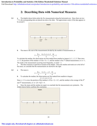
  • 1. 29 2: Describing Data with Numerical Measures 2.1 a The dotplot shown below plots the five measurements along the horizontal axis. Since there are two “1”s, the corresponding dots are placed one above the other. The approximate center of the data appears to be around 1. 543210 Dotplot median mode mean b The mean is the sum of the measurements divided by the number of measurements, or 0 5 1 1 3 10 2 5 5 ix x n ∑ + + + + = = = = To calculate the median, the observations are first ranked from smallest to largest: 0, 1, 1, 3, 5. Then since 5n = , the position of the median is 0.5( 1) 3n + = , and the median is the 3rd ranked measurement, or 1m = . The mode is the measurement occurring most frequently, or mode = 1. c The three measures in part b are located on the dotplot. Since the median and mode are to the left of the mean, we conclude that the measurements are skewed to the right. 2.2 a The mean is 3 2 5 32 4 8 8 ix x n ∑ + + + = = = = b To calculate the median, the observations are first ranked from smallest to largest: 2, 3, 3, 4, 4, 5, 5, 6 Since 8n = is even, the position of the median is 0.5( 1) 4.5n + = , and the median is the average of the 4th and 5th measurements, or ( )4 4 2 4m = + = . c Since the mean and the median are equal, we conclude that the measurements are symmetric. The dotplot shown below confirms this conclusion. 65432 Dotplot Introduction to Probability and Statistics 13th Edition Mendenhall Solutions Manual Full Download: http://alibabadownload.com/product/introduction-to-probability-and-statistics-13th-edition-mendenhall-solutions-m This sample only, Download all chapters at: alibabadownload.com
  • 2. 30 2.3 a 58 5.8 10 ix x n ∑ = = = b The ranked observations are: 2, 3, 4, 5, 5, 6, 6, 8, 9, 10. Since 10n = , the median is halfway between the 5th and 6th ordered observations, or ( )5 6 2 5.5m = + = . c There are two measurements, 5 and 6, which both occur twice. Since this is the highest frequency of occurrence for the data set, we say that the set is bimodal with modes at 5 and 6. 2.4 a 9455 2363.75 4 ix x n ∑ = = = b 8280 2070 4 ix x n ∑ = = = c The average premium cost in several different cities is not as important to the consumer as the average cost for a variety of consumers in his or her geographical area. 2.5 a Although there may be a few households who own more than one DVD player, the majority should own either 0 or 1. The distribution should be slightly skewed to the right. b Since most households will have only one DVD player, we guess that the mode is 1. c The mean is 1 0 1 27 1.08 25 25 ix x n ∑ + + + = = = = To calculate the median, the observations are first ranked from smallest to largest: There are six 0s, thirteen 1s, four 2s, and two 3s. Then since 25n = , the position of the median is 0.5( 1) 13n + = , which is the 13th ranked measurement, or 1m = . The mode is the measurement occurring most frequently, or mode = 1. d The relative frequency histogram is shown below, with the three measures superimposed. Notice that the mean falls slightly to the right of the median and mode, indicating that the measurements are slightly skewed to the right. VCRs Relativefrequency 3210 10/25 5/25 0 median mode mean 2.6 a The stem and leaf plot below was generated by Minitab. It is skewed to the right. Stem-and-Leaf Display: Revenues Stem-and-leaf of Revenues N = 10 Leaf Unit = 10000 2 0 33 (4) 0 5555 4 0 4 0 889 1 1 1 1 1 1 1 1 1 1 9
  • 3. 31 b The mean is 192604 91134 38416 736951 73,695.10 10 10 ix x n ∑ + + + = = = = To calculate the median, notice that the observations are already ranked from smallest to largest. Then since 10n = , the position of the median is 0.5( 1) 5.5n + = , the average of the 5th and 6th ranked measurements or ( )54848 52620 2 53,734m = + = . c Since the mean is strongly affected by outliers, the median would be a better measure of center for this data set. 2.7 It is obvious that any one family cannot have 2.5 children, since the number of children per family is a quantitative discrete variable. The researcher is referring to the average number of children per family calculated for all families in the United States during the 1930s. The average does not necessarily have to be integer-valued. 2.8 a Similar to previous exercises. The mean is 0.99 1.92 0.66 12.55 0.896 14 14 ix x n ∑ + + + = = = = b To calculate the median, rank the observations from smallest to largest. The position of the median is 0.5( 1) 7.5n + = , and the median is the average of the 7th and 8th ranked measurement or ( )0.67 0.69 2 0.68m = + = . c Since the mean is slightly larger than the median, the distribution is slightly skewed to the right. 2.9 The distribution of sports salaries will be skewed to the right, because of the very high salaries of some sports figures. Hence, the median salary would be a better measure of center than the mean. 2.10 a Similar to previous exercises. 2150 215 10 ix x n ∑ = = = b The ranked observations are shown below: 175 225 185 230 190 240 190 250 200 265 The position of the median is 0.5( 1) 5.5n + = and the median is the average of the 5th and 6th observation or 200 225 212.5 2 + = c Since there are no unusually large or small observations to affect the value of the mean, we would probably report the mean or average time on task. 2.11 a Similar to previous exercises. 85 4.72 18 ix x n ∑ = = = The ranked observations are: 1 1 3 6 12 1 1 4 7 16 1 2 4 7 1 2 5 11 The median is the average of the 9th and 10th observations or
  • 4. 32 m = (3 + 4)/2 = 3.5 and the mode is the most frequently occurring observation—mode = 1. b Since the mean is larger than the median, the data are skewed to the right. c The dotplot is shown below. The distribution is skewed to the right. 161412108642 Starbucks Dotplot of Starbucks 2.12 a 19850 1985 10 ix x n ∑ = = = b The ranked data are: 1200, 1300, 1350, 1500, 1800, 2000, 2200, 2600, 2900, 3000 and the median is the average of the 5th and 6th observations or 1800 2000 1900 2 m + = = c Average cost would not be as important as many other variables, such as picture quality, sound quality, size, lowest cost for the best quality, and many other considerations. 2.13 a 12 2.4 5 ix x n ∑ = = = b Create a table of differences, ( )ix x− and their squares, ( ) 2 ix x− . ix ix x− ( ) 2 ix x− 2 –0.4 0.16 1 –1.4 1.96 1 –1.4 1.96 3 0.6 0.36 5 2.6 6.76 Total 0 11.20 Then ( ) 2 2 2 2 (2 2.4) (5 2.4) 11.20 2.8 1 4 4 ix x s n ∑ − − + + − = = = = − c The sample standard deviation is the positive square root of the variance or 2 2.8 1.673s s= = = d Calculate 2 2 2 2 2 1 5 40ix∑ = + + + = . Then ( ) ( ) 2 2 2 2 12 40 11.25 2.8 1 4 4 i i x x ns n ∑ ∑ − − = = = = − and 2 2.8 1.673s s= = = . The results of parts a and b are identical.
  • 5. 33 2.14 The results will vary from student to student, depending on their particular type of calculator. The results should agree with Exercise 2.13. 2.15 a The range is 4 1 3R = − = . b 17 2.125 8 ix x n ∑ = = = c Calculate 2 2 2 2 4 1 2 45ix∑ = + + + = . Then ( ) ( ) 2 2 2 2 17 45 8.8758 1.2679 1 7 7 i i x x ns n ∑ ∑ − − = = = = − and 2 1.2679 1.126s s= = = . 2.16 a The range is 6 1 5R = − = . b 31 3.875 8 ix x n ∑ = = = c Calculate 2 2 2 2 3 1 5 137ix∑ = + + + = . Then ( ) ( ) 2 2 2 2 31 137 16.8758 2.4107 1 7 7 i i x x ns n ∑ ∑ − − = = = = − and 2 2.4107 1.55s s= = = . d The range, 5R = , is 5 1.55 3.23= standard deviations. 2.17 a The range is 2.39 1.28 1.11R = − = . b Calculate 2 2 2 2 1.28 2.39 1.51 15.415ix∑ = + + + = . Then ( ) ( ) 2 2 2 2 8.56 15.415 .760285 .19007 1 4 4 i i x x ns n ∑ ∑ − − = = = = − and 2 .19007 .436s s= = = c The range, 1.11R = , is 1.11 .436 2.5= standard deviations. 2.18 a The range is 343.50 162.64 180.86R = − = . b 2940.2 245.02 12 ix x n ∑ = = = c Calculate 2 2 2 2 266.63 163.41 230.46 763773.912ix∑ = + + + = . Then ( ) ( ) 2 2 2 2 2940.2 763773.912 12 3943.264424 1 11 i i x x ns n ∑ ∑ − − = = = − and 2 3943.264424 62.795s s= = = . 2.19 a The range of the data is 6 1 5R = − = and the range approximation with 10n = is 1.67 3 R s ≈ = b The standard deviation of the sample is ( ) ( ) 2 2 2 2 32 130 10 3.0667 1.751 1 9 i i x x ns s n ∑ ∑ − − = = = = = − which is very close to the estimate for part a. c-e From the dotplot on the next page, you can see that the data set is not mound-shaped. Hence you can use Tchebysheff’s Theorem, but not the Empirical Rule to describe the data.
  • 6. 34 654321 Dotplot 2.20 a First calculate the intervals: 36 3 or 33 to 39 2 36 6 or 30 to 42 3 36 9 or 27 to 45 x s x s x s ± = ± ± = ± ± = ± According to the Empirical Rule, approximately 68% of the measurements will fall in the interval 33 to 39; approximately 95% of the measurements will fall between 30 and 42; approximately 99.7% of the measurements will fall between 27 and 45. b If no prior information as to the shape of the distribution is available, we use Tchebysheff’s Theorem. We would expect at least ( )2 1 1 1 0− = of the measurements to fall in the interval 33 to 39; at least ( )2 1 1 2 3 4− = of the measurements to fall in the interval 30 to 42; at least ( )2 1 1 3 8 9− = of the measurements to fall in the interval 27 to 45. 2.21 a The interval from 40 to 60 represents 50 10μ σ± = ± . Since the distribution is relatively mound- shaped, the proportion of measurements between 40 and 60 is 68% according to the Empirical Rule and is shown below. b Again, using the Empirical Rule, the interval 2 50 2(10)μ σ± = ± or between 30 and 70 contains approximately 95% of the measurements.
  • 7. 35 c Refer to the figure below. Since approximately 68% of the measurements are between 40 and 60, the symmetry of the distribution implies that 34% of the measurements are between 50 and 60. Similarly, since 95% of the measurements are between 30 and 70, approximately 47.5% are between 30 and 50. Thus, the proportion of measurements between 30 and 60 is 0.34 0.475 0.815+ = d From the figure in part a, the proportion of the measurements between 50 and 60 is 0.34 and the proportion of the measurements which are greater than 50 is 0.50. Therefore, the proportion that are greater than 60 must be 0.5 0.34 0.16− = 2.22 Since nothing is known about the shape of the data distribution, you must use Tchebysheff’s Theorem to describe the data. a The interval from 60 to 90 represents 3μ σ± which will contain at least 8/9 of the measurements. b The interval from 65 to 85 represents 2μ σ± which will contain at least 3/4 of the measurements. c The value 65x = lies two standard deviations below the mean. Since at least 3/4 of the measurements are within two standard deviation range, at most 1/4 can lie outside this range, which means that at most 1/4 can be less than 65. 2.23 a The range of the data is 1.1 0.5 0.6R = − = and the approximate value of s is 0.2 3 R s ≈ = b Calculate 7.6ix∑ = and 2 6.02ix∑ = , the sample mean is 7.6 .76 10 ix x n ∑ = = = and the standard deviation of the sample is ( ) ( ) 2 2 2 2 7.6 6.02 0.24410 0.165 1 9 9 i i x x ns s n ∑ ∑ − − = = = = = − which is very close to the estimate from part a.
  • 8. 36 2.24 a The stem and leaf plot generated by Minitab shows that the data is roughly mound-shaped. Note however the gap in the center of the distribution and the two measurements in the upper tail. Stem-and-Leaf Display: Weight Stem-and-leaf of Weight N = 27 Leaf Unit = 0.010 1 7 5 2 8 3 6 8 7999 8 9 23 13 9 66789 13 10 (3) 10 688 11 11 2244 7 11 788 4 12 4 3 12 8 2 13 2 13 8 1 14 1 b Calculate 28.41ix∑ = and 2 30.6071ix∑ = , the sample mean is 28.41 1.052 27 ix x n ∑ = = = and the standard deviation of the sample is ( ) ( ) 2 2 2 2 28.41 30.6071 27 0.166 1 26 i i x x ns s n ∑ ∑ − − = = = = − c The following table gives the actual percentage of measurements falling in the intervals x ks± for 1,2,3k = . k x ks± Interval Number in Interval Percentage 1 1.052 0.166± 0.866 to 1.218 21 78% 2 1.052 0.332± 0.720 to 1.384 26 96% 3 1.052 0.498± 0.554 to 1.550 27 100% d The percentages in part c do not agree too closely with those given by the Empirical Rule, especially in the one standard deviation range. This is caused by the lack of mounding (indicated by the gap) in the center of the distribution. e The lack of any one-pound packages is probably a marketing technique intentionally used by the supermarket. People who buy slightly less than one-pound would be drawn by the slightly lower price, while those who need exactly one-pound of meat for their recipe might tend to opt for the larger package, increasing the store’s profit. 2.25 According to the Empirical Rule, if a distribution of measurements is approximately mound-shaped, a approximately 68% or 0.68 of the measurements fall in the interval 12 2.3 or 9.7 to 14.3μ σ± = ± b approximately 95% or 0.95 of the measurements fall in the interval 2 12 4.6 or 7.4 to 16.6μ σ± = ± c approximately 99.7% or 0.997 of the measurements fall in the interval 3 12 6.9 or 5.1 to 18.9μ σ± = ± Therefore, approximately 0.3% or 0.003 will fall outside this interval.
  • 9. 37 2.26 a The stem and leaf plots are shown below. The second set has a slightly higher location and spread. Stem-and-Leaf Display: Method 1, Method 2 Stem-and-leaf of Method 1 N = 10 Stem-and-leaf of Method 2 N = 10 Leaf Unit = 0.00010 Leaf Unit = 0.00010 1 10 0 3 11 00 1 11 0 4 12 0 3 12 00 (4) 13 0000 5 13 00 2 14 0 5 14 0 1 15 0 4 15 00 2 16 0 1 17 0 b Method 1: Calculate 0.125ix∑ = and 2 0.001583ix∑ = . Then 0.0125ix x n ∑ = = and ( ) ( ) 2 2 2 2 0.125 0.001583 10 0.00151 1 9 i i x x ns s n ∑ ∑ − − = = = = − Method 2: Calculate 0.138ix∑ = and 2 0.001938ix∑ = . Then 0.0138ix x n ∑ = = and ( ) ( ) 2 2 2 2 0.138 0.001938 10 0.00193 1 9 i i x x ns s n ∑ ∑ − − = = = = − The results confirm the conclusions of part a. 2.27 a The center of the distribution should be approximately halfway between 0 and 9 or ( )0 9 2 4.5+ = . b The range of the data is 9 0 9R = − = . Using the range approximation, 4 9 4 2.25s R≈ = = . c Using the data entry method the students should find 4.586x = and 2.892s = , which are fairly close to our approximations. 2.28 a Similar to previous exercises. The intervals, counts and percentages are shown in the table. k x ks± Interval Number in Interval Percentage 1 4.586 2.892± 1.694 to 7.478 43 61% 2 4.586 5.784± –1.198 to 10.370 70 100% 3 4.586 8.676± –4.090 to 13.262 70 100% b The percentages in part a do not agree with those given by the Empirical Rule. This is because the shape of the distribution is not mound-shaped, but flat. 2.29 a Although most of the animals will die at around 32 days, there may be a few animals that survive a very long time, even with the infection. The distribution will probably be skewed right. b Using Tchebysheff’s Theorem, at least 3/4 of the measurements should be in the interval 32 72μ σ± ⇒ ± or 0 to 104 days. 2.30 a The value of x is 32 36 4μ σ− = − = − . b The interval is 32 36μ σ± ± should contain approximately ( )100 68 34%− = of the survival times, of which 17% will be longer than 68 days and 17% less than –4 days. c The latter is clearly impossible. Therefore, the approximate values given by the Empirical Rule are not accurate, indicating that the distribution cannot be mound-shaped.
  • 10. 38 2.31 a We choose to use 12 classes of length 1.0. The tally and the relative frequency histogram follow. Class i Class Boundaries Tally fi Relative frequency, fi/n 1 2 to < 3 1 1 1/70 2 3 to < 4 1 1 1/70 3 4 to < 5 111 3 3/70 4 5 to < 6 11111 5 5/70 5 6 to < 7 11111 5 5/70 6 7 to < 8 11111 11111 11 12 12/70 7 8 to < 9 11111 11111 11111 111 18 18/70 8 9 to < 10 11111 11111 11111 15 15/70 9 10 to < 11 11111 1 6 6/70 10 11 to < 12 111 3 3/70 11 12 to < 13 0 0 12 13 to < 14 1 1 1/70 TREES Relativefrequency 15105 20/70 10/70 0 b Calculate 70, 541in x= ∑ = and 2 4453ix∑ = . Then 541 7.729 70 ix x n ∑ = = = is an estimate of μ . c The sample standard deviation is ( ) ( ) 2 2 2 541 4453 70 3.9398 1.985 1 69 i i x x ns n ∑ ∑ − − = = = = − The three intervals, x ks± for 1,2,3k = are calculated below. The table shows the actual percentage of measurements falling in a particular interval as well as the percentage predicted by Tchebysheff’s Theorem and the Empirical Rule. Note that the Empirical Rule should be fairly accurate, as indicated by the mound- shape of the histogram in part a. k x ks± Interval Fraction in Interval Tchebysheff Empirical Rule 1 7.729 1.985± 5.744 to 9.714 50/70 = 0.71 at least 0 0.68≈ 2 7.729 3.970± 3.759 to 11.699 67/70 = 0.96 at least 0.75 0.95≈ 3 7.729 5.955± 1.774 to 13.684 70/70 = 1.00 at least 0.89 0.997≈ 2.32 a Calculate 1.92 0.53 1.39R = − = so that 4 1.39 4 0.3475s R≈ = = . b Calculate 14, 12.55in x= ∑ = and 2 13.3253ix∑ = . Then ( ) ( ) 2 2 2 2 12.55 13.3253 14 0.1596 1 13 i i x x ns n ∑ ∑ − − = = = − and 0.15962 0.3995s = = which is fairly close to the approximate value of s from part a.
  • 11. 39 2.33 a-b Calculate 93 51 42R = − = so that 4 42 4 10.5s R≈ = = . c Calculate 30, 2145in x= ∑ = and 2 158,345ix∑ = . Then ( ) ( ) 2 2 2 2 2145 158,345 30 171.6379 1 29 i i x x ns n ∑ ∑ − − = = = − and 171.6379 13.101s = = which is fairly close to the approximate value of s from part b. d The two intervals are calculated below. The proportions agree with Tchebysheff’s Theorem, but are not to close to the percentages given by the Empirical Rule. (This is because the distribution is not quite mound-shaped.) k x ks± Interval Fraction in Interval Tchebysheff Empirical Rule 2 71.5 26.20± 45.3 to 97.7 30/30 = 1.00 at least 0.75 0.95≈ 3 71.5 39.30± 32.2 to 110.80 30/30 = 1.00 at least 0.89 0.997≈ 2.34 a Answers will vary. A typical histogram is shown below. The distribution is skewed to the right. 1612840 .35 .30 .25 .20 .15 .10 .05 0 Kids Relativefrequency b Calculate 42, 151in x= ∑ = and 2 897ix∑ = . Then ( ) ( ) 2 2 2 2 151 3.60, 42 151 897 42 8.63705 1 41 i i i x x n x x ns n ∑ = = = ∑ ∑ − − = = = − and 8.63705 2.94s = = c The three intervals, x ks± for 1,2,3k = are calculated below. The table shows the actual percentage of measurements falling in a particular interval as well as the percentage predicted by Tchebysheff’s Theorem and the Empirical Rule. Note that the Empirical Rule is not very accurate for the first interval, since the histogram in part a is skewed. k x ks± Interval Fraction in Interval Tchebysheff Empirical Rule 1 3.60 2.94± .66 to 6.54 32/42 = .76 at least 0 0.68≈ 2 3.60 5.88± −2.28 to 9.48 40/42 = .95 at least 0.75 0.95≈ 3 3.60 8.82± −5.22 to 12.42 41/42 = .976 at least 0.89 0.997≈ 2.35 a Calculate 2.39 1.28 1.11R = − = so that 2.5 1.11 2.5 .444s R≈ = = . b In Exercise 2.17, we calculated 8.56ix∑ = and 2 2 2 2 1.28 2.39 1.51 15.415ix∑ = + + + = . Then ( ) ( ) 2 2 2 2 8.56 15.451 .760285 .19007 1 4 4 i i x x ns n ∑ ∑ − − = = = = −
  • 12. 40 and 2 .19007 .436s s= = = , which is very close to our estimate in part a. 2.36 a Answers will vary. A typical stem and leaf plot is generated by Minitab. Stem-and-Leaf Display: Favre Stem-and-leaf of Favre N = 16 Leaf Unit = 1.0 1 0 5 1 1 4 1 579 (8) 2 01222244 4 2 568 1 3 1 b Calculate 16, 343in x= ∑ = and 2 7875ix∑ = . Then 343 21.44 16 ix x n ∑ = = = , ( ) ( ) 2 2 2 2 343 7875 16 34.79583 1 15 i i x x ns n ∑ ∑ − − = = = − and 2 34.795833 5.90s s= = = . c Calculate 2 21.44 11.80 or 9.64 to 33.24.x s± ⇒ ± From the original data set, 15 of the 16 measurements, or about 94% fall in this interval. 2.37 a Calculate 15, 21in x= ∑ = and 2 49ix∑ = . Then 21 1.4 15 ix x n ∑ = = = and ( ) ( ) 2 2 2 2 21 49 15 1.4 1 14 i i x x ns n ∑ ∑ − − = = = − b Using the frequency table and the grouped formulas, calculate 0(4) 1(5) 2(2) 3(4) 21i ix f∑ = + + + = 2 2 2 2 2 0 (4) 1 (5) 2 (2) 3 (4) 49i ix f∑ = + + + = Then, as in part a, 21 1.4 15 i ix f x n ∑ = = = ( ) ( ) 2 2 2 2 21 49 15 1.4 1 14 i i i i x f x f ns n ∑ ∑ − − = = = − 2.38 Use the formulas for grouped data given in Exercise 2.37. Calculate 17, 79i in x f= ∑ = , and 2 393i ix f∑ = . Then, 79 4.65 17 i ix f x n ∑ = = = ( ) ( ) 2 2 2 2 79 393 17 1.6176 1 16 i i i i x f x f ns n ∑ ∑ − − = = = − and 1.6176 1.27s = = 2.39 a The data in this exercise have been arranged in a frequency table. xi 0 1 2 3 4 5 6 7 8 9 10 fi 10 5 3 2 1 1 1 0 0 1 1 Using the frequency table and the grouped formulas, calculate 0(10) 1(5) 10(1) 51i ix f∑ = + + + =
  • 13. 41 2 2 2 2 0 (10) 1 (5) 10 (1) 293i ix f∑ = + + + = Then 51 2.04 25 i ix f x n ∑ = = = ( ) ( ) 2 2 2 2 51 293 25 7.873 1 24 i i i i x f x f ns n ∑ ∑ − − = = = − and 7.873 2.806s = = . b-c The three intervals x ks± for 1,2,3k = are calculated in the table along with the actual proportion of measurements falling in the intervals. Tchebysheff’s Theorem is satisfied and the approximation given by the Empirical Rule are fairly close for 2k = and 3k = . k x ks± Interval Fraction in Interval Tchebysheff Empirical Rule 1 2.04 2.806± –0.766 to 4.846 21/25 = 0.84 at least 0 0.68≈ 2 2.04 5.612± –3.572 to 7.652 23/25 = 0.92 at least 0.75 0.95≈ 3 2.04 8.418± –6.378 to 10.458 25/25 = 1.00 at least 0.89 0.997≈ 2.40 The sorted data set, along with the positions of the quartiles and the quartiles themselves are shown in the table. Sorted Data Set n Position of Q1 Position of Q3 Lower quartile, Q1 Upper quartile, Q3 .13, 16, .21, .28, .34, .76, .88 7 .25(8) = 2 .75(8) = 6 .16 .76 1.0, 1.7, 2.0, 2.1, 2.3, 2.8, 2.9, 4.4, 5.1, 6.5, 8.8 11 .25(12) = 3 .75(12) = 9 2.0 5.1 2.41 The data have already been sorted. Find the positions of the quartiles, and the measurements that are just above and below those positions. Then find the quartiles by interpolation. Sorted Data Set Position of Q1 Above and below Q1 Position of Q3 Above and below Q3 1, 1.5, 2, 2, 2.2 .25(6) = 1.5 1 and 1.5 1.25 .75(6) = 4.5 2 and 2.2 2.1 0, 1.7, 1.8, 3.1, 3.2, 7, 8, 8.8, 8.9, 9, 10 .25(12) = 3 None 1.8 .75(12) = 9 None 8.9 .23, .30, .35, .41, .56, .58, .76, .80 .25(9) = 2.25 .30 and .35 .30 + .25(.05) = .3125 .75(9) = 6.75 .58 and .76 .58 + .75(.18) = .7150 2.42 The ordered data are: 0, 1, 3, 4, 4, 5, 6, 6, 7, 7, 8 a With 12n = , the median is in position 0.5( 1) 6.5n + = , or halfway between the 6th and 7th observations. The lower quartile is in position 0.25( 1) 3.25n + = (one-fourth of the way between the 3rd and 4th observations) and the upper quartile is in position 0.75( 1) 9.75n + = (three-fourths of the way between the 9th and 10th observations). Hence, ( ) 15 6 2 5.5, 3 0.25(4 3) 3.25m Q= + = = + − = and 3 6 0.75(7 6) 6.75Q = + − = . Then the five-number summary is Min Q1 Median Q3 Max 0 3.25 5.5 6.75 8 and
  • 14. 42 3 1 6.75 3.25 3.50IQR Q Q= − = − = b Calculate 12, 57in x= ∑ = and 2 337ix∑ = . Then 57 4.75 12 ix x n ∑ = = = and the sample standard deviation is ( ) ( ) 2 2 2 57 337 12 6.022727 2.454 1 11 i i x x ns n ∑ ∑ − − = = = = − c For the smaller observation, 0x = , 0 4.75 -score 1.94 2.454 x x z s − − = = = − and for the largest observation, 8x = , 8 4.75 -score 1.32 2.454 x x z s − − = = = Since neither z-score exceeds 2 in absolute value, none of the observations are unusually small or large. 2.43 The ordered data are: 0, 1, 5, 6, 7, 8, 9, 10, 12, 12, 13, 14, 16, 19, 19 With 15n = , the median is in position 0.5( 1) 8n + = , so that 10m = . The lower quartile is in position 0.25( 1) 4n + = so that 1 6Q = and the upper quartile is in position 0.75( 1) 12n + = so that 3 14Q = . Then the five-number summary is Min Q1 Median Q3 Max 0 6 10 14 19 and 3 1 14 6 8IQR Q Q= − = − = . 2.44 The ordered data are: 12, 18, 22, 23, 24, 25, 25, 26, 26, 27, 28 For 11n = , the position of the median is 0.5( 1) 0.5(11 1) 6n + = + = and 25m = . The positions of the quartiles are 0.25( 1) 3n + = and 0.75( 1) 9n + = , so that 1 322, 26,Q Q= = and 26 22 4IQR = − = . The lower and upper fences are: 1 3 1.5 22 6 16 1.5 26 6 32 Q IQR Q IQR − = − = + = + = The only observation falling outside the fences is 12x = which is identified as an outlier. The box plot is shown below. The lower whisker connects the box to the smallest value that is not an outlier, 18x = . The upper whisker connects the box to the largest value that is not an outlier or 28x = . x 3025201510
  • 15. 43 2.45 The ordered data are: 2, 3, 4, 5, 6, 6, 6, 7, 8, 9, 9, 10, 22 For 13n = , the position of the median is 0.5( 1) 0.5(13 1) 7n + = + = and 6m = . The positions of the quartiles are 0.25( 1) 3.5n + = and 0.75( 1) 10.5n + = , so that 1 34.5, 9,Q Q= = and 9 4.5 4.5IQR = − = . The lower and upper fences are: 1 3 1.5 4.5 6.75 2.25 1.5 9 6.75 15.75 Q IQR Q IQR − = − = − + = + = The value 22x = lies outside the upper fence and is an outlier. The box plot is shown below. The lower whisker connects the box to the smallest value that is not an outlier, which happens to be the minimum value, 2x = . The upper whisker connects the box to the largest value that is not an outlier or 10x = . x 2520151050 2.46 From Section 2.6, the 69th percentile implies that 69% of all students scored below your score, and only 31% scored higher. 2.47 a The ordered data are shown below: 1.70 101.00 209.00 264.00 316.00 445.00 1.72 118.00 218.00 278.00 318.00 481.00 5.90 168.00 221.00 286.00 329.00 485.00 8.80 180.00 241.00 314.00 397.00 85.40 183.00 252.00 315.00 406.00 For 28n = , the position of the median is 0.5( 1) 14.5n + = and the positions of the quartiles are 0.25( 1) 7.25n + = and 0.75( 1) 21.75n + = . The lower quartile is ¼ the way between the 7th and 8th measurements or 1 118 0.25(168 118) 130.5Q = + − = and the upper quartile is ¾ the way between the 21st and 22nd measurements or 3 316 0.75(318 316) 317.5Q = + − = . Then the five-number summary is Min Q1 Median Q3 Max 1.70 130.5 246.5 317.5 485 b Calculate 3 1 317.5 130.5 187IQR Q Q= − = − = . Then the lower and upper fences are: 1 3 1.5 130.5 280.5 150 1.5 317.5 280.5 598 Q IQR Q IQR − = − = − + = + =
  • 16. 44 The box plot is shown below. Since there are no outliers, the whiskers connect the box to the minimum and maximum values in the ordered set. Mercury 5004003002001000 c-d The boxplot does not identify any of the measurements as outliers, mainly because the large variation in the measurements cause the IQR to be large. However, the student should notice the extreme difference in the magnitude of the first four observations taken on young dolphins. These animals have not been alive long enough to accumulate a large amount of mercury in their bodies. 2.48 a See Exercise 2.24b. b For 1.38x = , 1.38 1.05 -score 1.94 0.17 x x z s − − = = = while for 1.41x = , 1.41 1.05 -score 2.12 0.17 x x z s − − = = = The value 1.41x = would be considered somewhat unusual, since its z-score exceeds 2 in absolute value. c For 27n = , the position of the median is 0.5( 1) 0.5(27 1) 14n + = + = and 1.06m = . The positions of the quartiles are 0.25( 1) 7n + = and 0.75( 1) 21n + = , so that 1 30.92, 1.17,Q Q= = and 1.17 0.92 0.25IQR = − = . The lower and upper fences are: 1 3 1.5 0.92 0.375 0.545 1.5 1.17 0.375 1.545 Q IQR Q IQR − = − = + = + = The box plot is shown below. Since there are no outliers, the whiskers connect the box to the minimum and maximum values in the ordered set. Weight 1.41.31.21.11.00.90.80.7
  • 17. 45 Since the median line is almost in the center of the box, the whiskers are nearly the same lengths, the data set is relatively symmetric. 2.49 a For 16n = , the position of the median is 0.5( 1) 8.5n + = and the positions of the quartiles are 0.25( 1) 4.25n + = and 0.75( 1) 12.75n + = . The lower quartile is ¼ the way between the 4th and 5th measurements and the upper quartile is ¾ the way between the 12th and 13th measurements. The sorted measurements are shown below. Favre: 5, 15, 17, 19, 20, 21, 22, 22, 22, 22, 24, 24, 25, 26, 28, 31 Peyton Manning: 14, 14, 20, 20, 21, 21, 21, 22, 25, 25, 25, 26, 27, 29, 30, 32 For Brett Favre, ( )22 22 2 22m = + = , 1 19 0.25(20 19) 19.25Q = + − = and 3 24 0.75(25 24) 24.75Q = + − = . For Peyton Manning, ( )22 25 2 23.50m = + = , 1 20 0.25(21 20) 20.25Q = + − = and 3 26 0.75(27 26) 26.75Q = + − = . Then the five-number summaries are Min Q1 Median Q3 Max Favre 5 19.25 22 24.75 31 Manning 14 20.25 23.5 26.75 32 b For Brett Favre, calculate 3 1 24.75 19.25 5.5IQR Q Q= − = − = . Then the lower and upper fences are: 1 3 1.5 19.25 8.25 11 1.5 24.75 8.25 33 Q IQR Q IQR − = − = + = + = and x = 5 is an outlier. For Peyton Manning, calculate 3 1 26.75 20.25 6.5IQR Q Q= − = − = . Then the lower and upper fences are: 1 3 1.5 20.25 9.75 10.5 1.5 26.75 9.75 36.5 Q IQR Q IQR − = − = + = + = and there are no outliers. The box plots are shown below. Manning Favre 3530252015105 Completed Passes c Answers will vary. The Favre distribution is relatively symmetric except for the one outlier; the Manning distribution is roughly symmetric, probably mound-shaped. The Manning distribution is slightly more variable; Manning has a higher median number of completed passes. 2.50 Answers will vary from student to student. The distribution is skewed to the right with three outliers (Truman, Cleveland and F. Roosevelt). The box plot is shown on the next page.
  • 18. 46 4003002001000 Vetoes 2.51 a Just by scanning through the 20 measurements, it seems that there are a few unusually small measurements, which would indicate a distribution that is skewed to the left. b The position of the median is 0.5( 1) 0.5(25 1) 10.5n + = + = and (120 127) / 2 123.5m = + = . The mean is 2163 108.15 20 ix x n ∑ = = = which is smaller than the median, indicate a distribution skewed to the left. c The positions of the quartiles are 0.25( 1) 5.25n + = and 0.75( 1) 15.75n + = , so that 1 365 .25(87 65) 70.5, 144 .75(147 144) 146.25,Q Q= − − = = + − = and 146.25 70.5 75.75IQR = − = . The lower and upper fences are: 1 3 1.5 70.5 113.625 43.125 1.5 146.25 113.625 259.875 Q IQR Q IQR − = − = − + = + = The box plot is shown below. There are no outliers. The long left whisker and the median line located to the right of the center of the box indicates that the distribution that is skewed to the left. 180160140120100806040200 Survival time 2.52 a The sorted data is: 162.64, 163.41, 187.16, 208.99, 219.41, 226.80 230.46, 266.63, 289.17, 306.55, 335.48, 343.50
  • 19. 47 The positions of the median and the quartiles are 0.5( 1) 6.5n + = , 0.25( 1) 3.25n + = and 0.75( 1) 9.75n + = , so that 1 3 (226.80 230.46) / 2 228.63 187.16 .25(208.99 187.16) 192.6175 289.17 .75(306.55 289.17) 302.205 m Q Q = + = = + − = = + − = and 302.205 192.6175 109.5875IQR = − = . The lower and upper fences are: 1 3 1.5 192.6175 164.38125 28.236 1.5 302.205 164.38125 466.586 Q IQR Q IQR − = − = + = + = There are no outliers, and the box plot is shown below. 350300250200150 Utility Bill b Because of the slightly longer right whisker and the median line to the left of center, the distribution is slightly skewed to the right. 2.53 Answers will vary. The student should notice the outliers in the female group, and that the median female temperature is higher than the median male temperature. 2.54 a Calculate 14, 367in x= ∑ = and 2 9641ix∑ = . Then 367 26.214 14 ix x n ∑ = = = and ( ) ( ) 2 2 2 367 9641 14 1.251 1 13 i i x x ns n ∑ ∑ − − = = = − b Calculate 14, 366in x= ∑ = and 2 9644ix∑ = . Then 366 26.143 14 ix x n ∑ = = = and ( ) ( ) 2 2 2 366 9644 14 2.413 1 13 i i x x ns n ∑ ∑ − − = = = − c The centers are roughly the same; the Sunmaid raisins appear slightly more variable. 2.55 a The ordered sets are shown below: Generic Sunmaid 24 25 25 25 26 22 24 24 24 24 26 26 26 26 27 25 25 27 28 28 27 28 28 28 28 28 29 30 For 14n = , the position of the median is 0.5( 1) 0.5(14 1) 7.5n + = + = and the positions of the quartiles are 0.25( 1) 3.75n + = and 0.75( 1) 11.25n + = , so that Generic: 1 326, 25, 27.25, and 27.25 25 2.25m Q Q IQR= = = = − = Sunmaid: 1 326, 24, 28, and 28 24 4m Q Q IQR= = = = − =
  • 20. 48 b Generic: Lower and upper fences are: 1 3 1.5 25 3.375 21.625 1.5 27.25 3.375 30.625 Q IQR Q IQR − = − = + = + = Sunmaid: Lower and upper fences are: 1 3 1.5 24 6 18 1.5 28 6 34 Q IQR Q IQR − = − = + = + = The box plots are shown below. There are no outliers. Raisins Generic Sunmaid 30292827262524232221 d If the boxes are not being underfilled, the average size of the raisins is roughly the same for the two brands. However, since the number of raisins is more variable for the Sunmaid brand, it would appear that some of the Sunmaid raisins are large while others are small. The individual sizes of the generic raisins are not as variable. 2.56 a Calculate the range as 15 1 14R = − = . Using the range approximation, 4 14 4 3.5s R≈ = = . b Calculate 25, 155.5in x= ∑ = and 2 1260.75ix∑ = . Then 155.5 6.22 25 ix x n ∑ = = = and ( ) ( ) 2 2 2 155.5 1260.75 25 3.497 1 24 i i x x ns n ∑ ∑ − − = = = − which is very close to the approximation found in part a. c Calculate 2 6.22 6.994x s± = ± or –0.774 to 13.214. From the original data, 24 measurements or ( )24 25 100 96%= of the measurements fall in this interval. This is close to the percentage given by the Empirical Rule. 2.57 a The largest observation found in the data from Exercise 1.26 is 32.3, while the smallest is 0.2. Therefore the range is 32.3 0.2 32.1R = − = . b Using the range, the approximate value for s is: 4 32.1 4 8.025s R≈ = = . c Calculate 50, 418.4in x= ∑ = and 2 6384.34ix∑ = . Then ( ) ( ) 2 2 2 418.4 6384.34 50 7.671 1 49 i i x x ns n ∑ ∑ − − = = = −
  • 21. 49 2.58 a Refer to Exercise 2.57. Since 418.4ix∑ = , the sample mean is 418.4 8.368 50 ix x n ∑ = = = The three intervals of interest is shown in the following table, along with the number of observations which fall in each interval. k x ks± Interval Number in Interval Percentage 1 8.368 7.671± 0.697 to 16.039 37 74% 2 8.368 15.342± –6.974 to 23.710 47 94% 3 8.368 23.013± –14.645 to 31.381 49 98% b The percentages falling in the intervals do agree with Tchebysheff’s Theorem. At least 0 fall in the first interval, at least 3 4 0.75= fall in the second interval, and at least 8 9 0.89= fall in the third. The percentages are not too close to the percentages described by the Empirical Rule (68%, 95%, and 99.7%). c The Empirical Rule may be unsuitable for describing these data. The data distribution does not have a strong mound-shape (see the relative frequency histogram in the solution to Exercise 1.26), but is skewed to the right. 2.59 The ordered data are shown below. 0.2 2.0 4.3 8.2 14.7 0.2 2.1 4.4 8.3 16.7 0.3 2.4 5.6 8.7 18.0 0.4 2.4 5.8 9.0 18.0 1.0 2.7 6.1 9.6 18.4 1.2 3.3 6.6 9.9 19.2 1.3 3.5 6.9 11.4 23.1 1.4 3.7 7.4 12.6 24.0 1.6 3.9 7.4 13.5 26.7 1.6 4.1 8.2 14.1 32.3 Since 50n = , the position of the median is 0.5( 1) 25.5n + = and the positions of the lower and upper quartiles are 0.25( 1) 12.75n + = and 0.75( 1) 38.25n + = . Then ( ) 16.1 6.6 2 6.35, 2.1 0.75(2.4 2.1) 2.325m Q= + = = + − = and 3 12.6 0.25(13.5 12.6) 12.825Q = + − = . Then 12.825 2.325 10.5IQR = − = . The lower and upper fences are: 1 3 1.5 2.325 15.75 13.425 1.5 12.825 15.75 28.575 Q IQR Q IQR − = − = − + = + = and the box plot is shown below. There is one outlier, 32.3x = . The distribution is skewed to the right. TIME 35302520151050
  • 22. 50 2.60 a For 14n = , the position of the median is 0.5( 1) 7.5n + = and the positions of the quartiles are 0.25( 1) 3.75n + = and 0.75( 1) 11.25n + = . The lower quartile is ¾ the way between the 3rd and 4th measurements or 1 0.60 0.75(0.63 0.60) 0.6225Q = + − = and the upper quartile is ¼ the way between the 11th and 12th measurements or 3 1.12 0.25(1.23 1.12) 1.1475Q = + − = . Then the five-number summary is Min Q1 Median Q3 Max 0.53 0.6225 0.68 1.1475 1.92 b Calculate 3 1 1.1475 0.6225 0.5250IQR Q Q= − = − = . Then the lower and upper fences are: 1 3 1.5 0.6225 0.7875 0.165 1.5 1.1475 0.7875 1.935 Q IQR Q IQR − = − = − + = + = The box plot is shown below. Since there are no outliers, the whiskers connect the box to the minimum and maximum values in the ordered set. Prices 2.001.751.501.251.000.750.50 c Calculate 14, 12.55in x= ∑ = , 2 13.3253ix∑ = . Then 12.55 0.896 14 ix x n ∑ = = = and ( ) ( ) 2 2 2 12.55 13.3253 14 0.3995 1 13 i i x x ns n ∑ ∑ − − = = = − The z-score for 1.92x = is 1.92 0.896 2.56 0.3995 x x z s − − = = = which is somewhat unlikely. This observation does not appear as an outlier in the box plot. 2.61 First calculate the intervals: 0.17 0.01x s± = ± or 0.16 to 0.18 2 0.17 0.02x s± = ± or 0.15 to 0.19 3 0.17 0.03x s± = ± or 0.14 to 0.20 a If no prior information as to the shape of the distribution is available, we use Tchebysheff’s Theorem. We would expect at least ( )2 1 1 1 0− = of the measurements to fall in the interval 0.16 to 0.18; at least
  • 23. 51 ( )2 1 1 2 3 4− = of the measurements to fall in the interval 0.15 to 0.19; at least ( )2 1 1 3 8 9− = of the measurements to fall in the interval 0.14 to 0.20. b According to the Empirical Rule, approximately 68% of the measurements will fall in the interval 0.16 to 0.18; approximately 95% of the measurements will fall between 0.15 to 0.19; approximately 99.7% of the measurements will fall between 0.14 and 0.20. Since mound-shaped distributions are so frequent, if we do have a sample size of 30 or greater, we expect the sample distribution to be mound-shaped. Therefore, in this exercise, we would expect the Empirical Rule to be suitable for describing the set of data. c If the chemist had used a sample size of four for this experiment, the distribution would not be mound-shaped. Any possible histogram we could construct would be non-mound-shaped. We can use at most 4 classes, each with frequency 1, and we will not obtain a histogram that is even close to mound- shaped. Therefore, the Empirical Rule would not be suitable for describing 4n = measurements. 2.62 Since it is not obvious that the distribution of amount of chloroform per liter of water in various water sources is mound-shaped, we cannot make this assumption. Tchebysheff’s Theorem can be used, however, and the necessary intervals and fractions falling in these intervals are given in the table. k x ks± Interval Tchebysheff 1 34 53± –19 to 87 at least 0 2 34 106± –72 to 40 at least 0.75 3 34 159± –125 to 193 at least 0.89 2.63 The following information is available: 2 400, 600, 4900n x s= = = The standard deviation of these scores is then 70, and the results of Tchebysheff’s Theorem follow: k x ks± Interval Tchebysheff 1 600 70± 530 to 670 at least 0 2 600 140± 460 to 740 at least 0.75 3 600 210± 390 to 810 at least 0.89 If the distribution of scores is mound-shaped, we use the Empirical Rule, and conclude that approximately 68% of the scores would lie in the interval 530 to 670 (which is x s± ). Approximately 95% of the scores would lie in the interval 460 to 740. 2.64 a Calculate 10, 68.5in x= ∑ = , 2 478.375ix∑ = . Then 68.5 6.85 10 ix x n ∑ = = = and ( ) ( ) 2 2 2 68.5 478.375 10 1.008 1 9 i i x x ns n ∑ ∑ − − = = = − b The z-score for 8.5x = is 8.5 6.85 1.64 1.008 x x z s − − = = = This is not an unusually large measurement. c The most frequently recorded measurement is the mode or x = 7 hours of sleep. d For 10n = , the position of the median is 0.5( 1) 5.5n + = and the positions of the quartiles are 0.25( 1) 2.75n + = and 0.75( 1) 8.25n + = . The sorted data are: 5, 6, 6, 6.75, 7, 7, 7, 7.25, 8, 8.5 Then ( ) 17 7 2 7, 6 0.75(6 6) 6m Q= + = = + − = and 3 7.25 0.25(8 7.25) 7.4375Q = + − = .
  • 24. 52 Then 7.4375 6 1.4375IQR = − = and the lower and upper fences are: 1 3 1.5 6 2.15625 3.84 1.5 7.4375 2.15625 9.59 Q IQR Q IQR − = − = + = + = There are no outliers (confirming the results of part b) and the box plot is shown below. Hours of sleep 98765 2.65 a Max = 27, Min = 20.2 and the range is 27 20.2 6.8R = − = . b Answers will vary. A typical histogram is shown below. The distribution is slightly skewed to the left. mpg Percent 2726252423222120 .25 .20 .15 .10 .05 0 c Calculate 20, 479.2in x= ∑ = , 2 11532.82ix∑ = . Then 479.2 23.96 20 ix x n ∑ = = = ( ) ( ) 2 2 2 479.2 11532.82 20 2.694 1.641 1 19 i i x x ns n ∑ ∑ − − = = = = − d The sorted data is shown below: 20.2 21.3 22.2 22.7 22.9 23.1 23.2 23.6 23.7 24.2 24.4 24.4 24.6 24.7 24.7 24.9 25.3 25.9 26.2 27.0 The z-scores for x = 20.2 and x = 27 are 20.2 23.96 27 23.96 2.29 and 1.85 1.641 1.641 x x x x z z s s − − − − = = = − = = = Since neither of the z-scores are greater than 3 in absolute value, the measurements are not judged to be outliers.
  • 25. 53 e The position of the median is 0.5( 1) 10.5n + = and the median is m = (24.2 + 24.4)/2 = 24.3 f The positions of the quartiles are 0.25( 1) 5.25n + = and 0.75( 1) 15.75n + = . Then 1 22.9 0.25(23.1 22.9) 22.95Q = + − = and 3 24.7 0.75(24.9 24.7) 24.85.Q = + − = 2.66 Refer to Exercise 2.65. Calculate 24.85 22.95 1.9IQR = − = . The lower and upper fences are: 1 3 1.5 22.95 2.85 20.10 1.5 24.85 2.85 27.70 Q IQR Q IQR − = − = + = + = There are no outliers, which confirms the conclusion in Exercise 2.65. The box plot is shown below. mpg 2726252423222120 2.67 a The range is 71 40 31R = − = and the range approximation is 4 31 4 7.75s R≈ = = b Calculate 10, 592in x= ∑ = , 2 36014ix∑ = . Then 592 59.2 10 ix x n ∑ = = = ( ) ( ) 2 2 2 592 36014 10 107.5111 10.369 1 9 i i x x ns n ∑ ∑ − − = = = = − The sample standard deviation calculated above is of the same order as the approximated value found in part a. c The ordered set is: 40, 49, 52, 54, 59, 61, 67, 69, 70, 71 Since 10n = , the positions of m, Q1, and Q3 are 5.5, 2.75 and 8.25 respectively, and ( )59 61 2 60m = + = , 1 49 0.75(52 49) 51.25Q = + − = , 3 69.75Q = and 69.75 51.25 18.5IQR = − = . The lower and upper fences are: 1 3 1.5 51.25 27.75 23.5 1.5 69.75 27.75 97.50 Q IQR Q IQR − = − = + = + = and the box plot is shown on the next page. There are no outliers and the data set is slightly skewed left.
  • 26. 54 Bacteria 7570656055504540 2.68 The results of the Empirical Rule follow: k x ks± Interval Empirical Rule 1 420 5± 415 to 425 approximately 0.68 2 420 10± 410 to 430 approximately 0.95 3 420 15± 405 to 435 approximately 0.997 Notice that we are assuming that attendance follows a mound-shaped distribution and hence that the Empirical Rule is appropriate. 2.69 If the distribution is mound-shaped, then almost all of the measurements will fall in the interval 3μ σ± , which is an interval 6σ in length. That is, the range of the measurements should be approximately 6σ . In this case, the range is 800 200 600− = , so that 600 6 100σ ≈ = . 2.70 They are probably referring to the average number of times that men and women go camping per year. 2.71 The stem lengths are approximately normal with mean 15 and standard deviation 2.5. a In order to determine the percentage of roses with length less than 12.5, we must determine the proportion of the curve which lies within the shaded area in the figure below. Using the Empirical Rule, the proportion of the area between 12.5 and 15 is half of 0.68 or 0.34. Hence, the fraction below 12.5 would be 0.5 0.34 0.16− = or 16%. x 201512.5 0.4 0.3 0.2 0.1 0.0 34% 47.5% 16% b Refer to the figure shown above. Again we use the Empirical Rule. The proportion of the area between 12.5 and 15 is half of 0.68 or 0.34, while the proportion of the area between 15 and 20 is half of 0.95 or 0.475. The total area between 12.5 and 20 is then 0.34 + 0.475 = .815 or 81.5%. 2.72 a The range is 172 108 64R = − = and the range approximation is 4 64 4 16s R≈ = =
  • 27. 55 b Calculate 15, 2041in x= ∑ = , 2 281,807ix∑ = . Then 2041 136.07 15 ix x n ∑ = = = ( ) ( ) 2 2 2 2041 281,807 15 292.495238 17.102 1 14 i i x x ns n ∑ ∑ − − = = = = − c According to Tchebysheff’s Theorem, with k = 2, at least 3/4 or 75% of the measurements will lie within k = 2 standard deviations of the mean. For this data, the two values, a and b, are calculated as 2 136.07 2(17.10) 137.07 34.20x s± ⇒ ± ⇒ ± or a = 101.87 and b = 170.27. 2.73 The diameters of the trees are approximately mound-shaped with mean 14 and standard deviation 2.8. a The value x = 8.4 lies two standard deviations below the mean, while the value x = 22.4 is three standard deviations above the mean. Use the Empirical Rule. The fraction of trees with diameters between 8.4 and 14 is half of 0.95 or 0.475, while the fraction of trees with diameters between 14 and 22.4 is half of 0.997 or 0.4985. The total fraction of trees with diameters between 8.4 and 22.4 is 0.475 + 0.4985 = .9735 b The value x = 16.8 lies one standard deviation above the mean. Using the Empirical Rule, the fraction of trees with diameters between 14 and 16.8 is half of 0.68 or 0.34, and the fraction of trees with diameters greater than 16.8 is 0.5 0.34 .16− = 2.74 a The range is 19 4 15R = − = and the range approximation is 4 15 4 3.75s R≈ = = b Calculate 15, 175in x= ∑ = , 2 2237ix∑ = . Then 175 11.67 15 ix x n ∑ = = = ( ) ( ) 2 2 2 175 2237 15 13.95238 3.735 1 14 i i x x ns n ∑ ∑ − − = = = = − c Calculate the interval 2 11.67 2(3.735) 11.67 7.47x s± ⇒ ± ⇒ ± or 4.20 to 19.14. Referring to the original data set, the fraction of measurements in this interval is 14/15 = .93. 2.75 a It is known that duration times are approximately normal, with mean 75 and standard deviation 20. In order to determine the probability that a commercial lasts less than 35 seconds, we must determine the fraction of the curve which lies within the shaded area in the figure on the next page. Using the Empirical Rule, the fraction of the area between 35 and 75 is half of 0.95 or 0.475. Hence, the fraction below 35 would be 0.5 0.475 0.025− = .
  • 28. 56 b The fraction of the curve area that lies above the 55 second mark may again be determined by using the Empirical Rule. Refer to the figure in part a. The fraction between 55 and 75 is 0.34 and the fraction above 75 is 0.5. Hence, the probability that a commercial lasts longer than 55 seconds is 0.5 0.34 0.84+ = . 2.76 a The relative frequency histogram for these data is shown below. x Relativefrequency 86420 .7 .6 .5 .4 .3 .2 .1 0 b Refer to the formulas given in Exercise 2.37. Using the frequency table and the grouped formulas, calculate 2 100, 66, 234i i i in x f x f= ∑ = ∑ = . Then 66 0.66 100 i ix f x n ∑ = = = ( ) ( ) 2 2 2 2 66 234 100 1.9236 1 99 i i i i x f x f ns n ∑ ∑ − − = = = − and 1.9236 1.39s = = . c The three intervals, x ks± for 2,3k = are calculated in the table along with the actual proportion of measurements falling in the intervals. Tchebysheff’s Theorem is satisfied and the approximation given by the Empirical Rule are fairly close for 2k = and 3k = . k x ks± Interval Fraction in Interval Tchebysheff Empirical Rule 2 0.66 2.78± –2.12 to 3.44 95/100 = 0.95 at least 0.75 0.95≈ 3 0.66 4.17± –3.51 to 4.83 96/100 = 0.96 at least 0.89 0.997≈ 2.77 a The percentage of colleges that have between 145 and 205 teachers corresponds to the fraction of measurements expected to lie within two standard deviations of the mean. Tchebysheff’s Theorem states that this fraction will be at least ¾ or 75%.
  • 29. 57 b If the population is normally distributed, the Empirical Rule is appropriate and the desired fraction is calculated. Referring to the normal distribution shown below, the fraction of area lying between 175 and 190 is 0.34, so that the fraction of colleges having more than 190 teachers is 0.5 0.34 0.16− = . 2.78 We must estimate s and compare with the student’s value of 0.263. In this case, 20n = and the range is 17.4 16.9 0.5R = − = . The estimated value for s is then 4 0.5 4 0.125s R≈ = = which is less than 0.263. It is important to consider the magnitude of the difference between the “rule of thumb” and the calculated value. For example, if we were working with a standard deviation of 100, a difference of 0.142 would not be great. However, the student’s calculation is twice as large as the estimated value. Moreover, two standard deviations, or 2(0.263) 0.526= , already exceeds the range. Thus, the value 0.263s = is probably incorrect. The correct value of s is ( ) 2 2 117032.41 5851.95 20 0.0173 0.132 1 19 i i x x ns n ∑ ∑ − − = = = = − 2.79 Notice that two (Sosa and McGuire) of the four players have relatively symmetric distributions. The whiskers are the same length and the median line is close to the middle of the box. The variability of the distributions is similar for all four players, but Barry Bonds has a distribution with a long right whisker, meaning that there may be an unusually large number of homers during one of his seasons. The distribution for Babe Ruth is slightly different from the others. The median line to the right of middle indicates a distribution skewed to the left; that there were a few seasons in which his homerun total was unusually low. In fact, the median number of homeruns for the other three players are all about 34-35, while Babe Ruth’s median number of homeruns is closer to 40. 2.80 a Use the information in the exercise. For 2001, 16.5IQR = , and the upper fence is 3 1.5 41.50 24.75 66.25Q IQR+ = + = For 2006, 20IQR = , and the upper fence is 3 1.5 45.00 30.00 75.00Q IQR+ = + = b The upper fence is different in 2006, so that the record number of homers, x = 73 is no longer an outlier, although it is still the most homers ever hit in a single season! 2.81 a Calculate 50, 418in x= ∑ = , so that 418 8.36 50 ix x n ∑ = = = . b The position of the median is .5( 1) 25.5n + = and m = (4 + 4)/2 = 4. c Since the mean is larger than the median, the distribution is skewed to the right.
  • 30. 58 d Since 50n = , the positions of Q1 and Q3 are .25(51) = 12.75 and .75(51) = 38.25, respectively Then 1 0 0.75(1 0) 12.75Q = + − = , 3 17 .25(19 17) 17.5Q = + − = and 17.5 .75 16.75IQR = − = . The lower and upper fences are: 1 3 1.5 .75 25.125 24.375 1.5 17.5 25.125 42.625 Q IQR Q IQR − = − = − + = + = and the box plot is shown below. There are no outliers and the data is skewed to the right. Age (Years) 403020100 2.82 Each bulleted statement produces a percentile. x = hourly pay for salespeople. The value 10.41x = is the 50th percentile or the median. x = hours worked per week by workers ages 16 and older. The value 40x = is the (100-69) = 31st percentile. x = salary for Associate Professors of mathematics in the U.S.. The value 91,823x = is the 75th percentile or the upper quartile. 2.83 Answers will vary. Students should notice that the distribution of baseline measurements is relatively mound-shaped. Therefore, the Empirical Rule will provide a very good description of the data. A measurement which is further than two or three standard deviations from the mean would be considered unusual. 2.84 a Calculate 25, 104.9in x= ∑ = , 2 454.810ix∑ = . Then 104.9 4.196 25 ix x n ∑ = = = ( ) ( ) 2 2 2 104.9 454.810 25 .610 .781 1 24 i i x x ns n ∑ ∑ − − = = = = − b The ordered data set is shown below: 2.5 3.0 3.1 3.3 3.6 3.7 3.8 3.8 3.9 3.9 4.1 4.2 4.2 4.2 4.3 4.3 4.4 4.7 4.7 4.8 4.8 5.2 5.3 5.4 5.7 c The z-scores for x = 2.5 and x = 5.7 are 2.5 4.196 5.7 4.196 2.17 and 1.93 .781 .781 x x x x z z s s − − − − = = = − = = = Since neither of the z-scores are greater than 3 in absolute value, the measurements are not judged to be unusually large or small.
  • 31. 59 2.85 a For 25n = , the position of the median is 0.5( 1) 13n + = and the positions of the quartiles are 0.25( 1) 6.5n + = and 0.75( 1) 19.5n + = . Then m = 4.2, 1 (3.7 3.8) / 2 3.75Q = + = and 3 (4.7 4.8) / 2 4.75Q = + = .Then the five-number summary is Min Q1 Median Q3 Max 2.5 3.75 4.2 4.75 5.7 b-c Calculate 3 1 4.75 3.75 1IQR Q Q= − = − = . Then the lower and upper fences are: 1 3 1.5 3.75 1.5 2.25 1.5 4.75 1.5 6.25 Q IQR Q IQR − = − = + = + = There are no unusual measurements, and the box plot is shown below. Times 6.05.55.04.54.03.53.02.5 d Answers will vary. A stem and leaf plot, generated by Minitab, is shown below. The data is roughly mound-shaped. Stem-and-Leaf Display: Times Stem-and-leaf of Times N = 25 Leaf Unit = 0.10 1 2 5 4 3 013 10 3 678899 (7) 4 1222334 8 4 7788 4 5 234 1 5 7 2.86 a When the applet loads, the mean and median are shown in the upper left-hand corner: 6.6 and 6.0x m= = b When the largest value is changed to 13x = , 7.0 and 6.0x m= = . c When the largest value is changed to 33x = , 11.0 and 6.0x m= = . The mean is larger when there is one unusually large measurement. d Extremely large values cause the mean to increase, but not the median. 2.87 a-b As the value of x gets smaller, so does the mean. c The median does not change until the green dot is smaller than 10x = , at which point the green dot becomes the median. d The largest and smallest possible values for the median are 5 10m≤ ≤ . 2.88 a When the applet loads, the mean and median are shown in the upper left-hand corner: 31.6 and 32.0x m= = b When the smallest value is changed to 25x = , 31.2 and 32.0x m= = . c When the smallest value is changed to 5x = , 27.2 and 32.0x m= = . The mean is smaller when there is one unusually small measurement.
  • 32. 60 d 29.0x = e The largest and smallest possible values for the median are 32 34m≤ ≤ . f Extremely small values cause the mean to decrease, but not the median. 2.89 Answers will vary from student to student. Students should notice that, when the estimators are compared in the long run, the standard deviation when dividing by 1n − is closer to 29.2σ = . When dividing by n, the estimate is closer to 23.8. 2.90 a Answers will vary from student to student. Students should notice that, when the estimators are compared in the long run, the standard deviation when dividing by 1n − is closer to 29.2σ = . When dividing by n, the estimate is closer to 27.5. b When the sample size is larger, the estimate is not as far from the true value 29.2σ = . The difference between the two estimators is less noticeable. 2.91 The box plot shows a distribution that is skewed to the left, but with one outlier to the right of the other observations ( 520x = ). 2.92 The box plot shows a distribution that is slightly skewed to the right, with no outliers. The student should estimate values for m, Q1, and Q3 that are close to the true values: 1 312, 8.75, and 18.5m Q Q= = = . Case Study: The Boys of Summer 1 The Minitab computer package was used to analyze the data. In the printout below, various descriptive statistics as well as histograms and box plots are shown. 0.440.420.400.380.360.340.32 30 25 20 15 10 5 0 AVERAGE Frequency Histogram of National League Batting Champions 0.420.400.380.360.340.320.30 18 16 14 12 10 8 6 4 2 0 AVERAGE Frequency Histogram of American League Batting Champions
  • 33. 61 Descriptive Statistics: AVERAGE Variable LEAGUE N N* Mean SE Mean StDev Minimum Q1 Median AVERAGE 0 131 0 0.35878 0.00225 0.02575 0.31300 0.33900 0.35400 1 106 0 0.35753 0.00263 0.02703 0.30100 0.33675 0.35600 Variable LEAGUE Q3 Maximum AVERAGE 0 0.37200 0.43800 1 0.37725 0.42200 2 Notice that the mean percentage of hits is almost the same for the two leagues, but that the American League (1) is slightly more variable. American National 0.440.420.400.380.360.340.320.30 LEAGUE AVERAGE 3 The box plot shows that there are three outliers in the National League (0). 4 In summary, except for the two outliers, there is very little difference between the two leagues. Introduction to Probability and Statistics 13th Edition Mendenhall Solutions Manual Full Download: http://alibabadownload.com/product/introduction-to-probability-and-statistics-13th-edition-mendenhall-solutions-m This sample only, Download all chapters at: alibabadownload.com