SlideShare a Scribd company logo
1 of 127
The Arithmetic Mean
An arithmetic mean is a fancy term for what most people call an "average." When
someone says the average of 10 and 20 is 15, they are referring to the arithmetic mean.
The simplest definition of a mean is the following: Add up all the numbers you want to
average, and then divide by the number of items you just added.
For example, if you want to average 10, 20, and 27, first add them together to get
10+20+27= 57. Then divide by 3 because we have three values, and we get an
arithmetic mean (average) of 19.
Want a formal, mathematical expression of the arithmetic mean?
That's just a fancy way to say "the sum of k different numbers divided by k."
Check out a few example of the arithmetic mean to make sure you understand:
Example:
Find the arithmetic mean (average) of the following numbers: 9, 3, 7, 3, 8, 10, and 2.
Solution:
Add up all the numbers. Then divide by 7 because there are 7 different numbers.
Example:
Find the arithmetic mean of -4, 3, 18, 0, 0, and -10.
Solution:
Sum the numbers. Divide by 6 because there are 6 numbers.
The answer is 7/6, or 1.167
Geometric Mean
The geometric mean is NOT the arithmetic mean and it is NOT a simple average. It is
the nth root of the product of n numbers. That means you multiply a bunch of numbers
together, and then take the nth root, where n is the number of values you just multiplied.
Did that make sense? Here's a quick example:
Example:
What is the geometric mean of 2, 8 and 4?
Solution:
Multiply those numbers together. Then take the third root (cube root) because there are
3 numbers.
Naturally, the geometric mean can get very complicated. Here's a mathematical
definition of the geometric mean:
Remember that the capital PI symbol means to multiply a series of numbers. That
definition says to multiply k numbers and then take the kth root. One thing you should
know is that the geometric mean only works with positive numbers. Negative numbers
could result in imaginary results depending on how many negative numbers are in a set.
Typically this isn't a problem, because most uses of the geometric mean involve real
data, such as the length of physical objects or the number of people responding to a
survey.
Try a few more examples until you understand the geometric mean.
Example:
What is the geometric mean of 4, 9, 9, and 2?
Solution:
Just multiply the four numbers and take the 4th root:
The geometric mean between two numbers is:
The arithmetic mean between two numbers is:
Example: The cut-off frequencies of a phone line are f1 = 300 Hz
and f2 = 3300 Hz. What is the center frequency?
The center frequency is f0 = 995 Hz as geometric mean and
not f0 = 1800 Hz (arithmetic mean). What a difference!
The geometric mean of two numbers is the square root of their product.
The geometric mean of three numbers is the cubic root of their product.
The arithmetic mean is the sum of the numbers, divided by the quantity of the
numbers.
Other names for arithmetic mean: average, mean, arithmetic average.
In general, you can only take the geometric mean of positive numbers.
The geometric mean, by definition, is the nth root of the product of the n units in a data
set. For example, the geometric mean of 5, 7, 2, 1 is (5 × 7 × 2 × 1)1/4
= 2.893.
Alternatively, if you log transform each of the individual units the geometric will be the
exponential of the arithmetic mean of these log-transformed values. So, reusing the
example above, exp [ ( ln(5) + ln(7) + ln(2) + ln(1) ) / 4 ] = 2.893.
Geometric Mean
Arithmetic Mean
An arithmetic average is the sum of a series of numbers divided by the count of that
series of numbers.
If you were asked to find the class (arithmetic) average of test scores, you would simply
add up all the test scores of the students, and then divide that sum by the number of
students. For example, if five students took an exam and their scores were 60%, 70%,
80%, 90% and 100%, the arithmetic class average would be 80%.
This would be calculated as: (0.6 + 0.7 + 0.8 + 0.9 + 1.0) / 5 = 0.8.
The reason you use an arithmetic average for test scores is that each test score is an
independent event. If one student happens to perform poorly on the exam, the next
student's chances of doing poor (or well) on the exam isn't affected. In other words,
each student's score is independent of the all other students' scores. However, there
are some instances, particularly in the world of finance, where an arithmetic mean is not
an appropriate method for calculating an average.
Consider your investment returns, for example. Suppose you have invested your
savings in the stock market for five years. If your returns each year were 90%, 10%,
20%, 30% and -90%, what would your average return be during this period? Well,
taking the simple arithmetic average, you would get an answer of 12%. Not too shabby,
you might think.
However, when it comes to annual investment returns, the numbers are not
independent of each other. If you lose a ton of money one year, you have that much
less capital to generate returns during the following years, and vice versa. Because of
this reality, we need to calculate the geometric average of your investment returns in
order to get an accurate measurement of what your actual average annual return over
the five-year period is.
To do this, we simply add one to each number (to avoid any problems with negative
percentages). Then, multiply all the numbers together, and raise their product to the
power of one divided by the count of the numbers in the series. And you're finished -
just don't forget to subtract one from the result!
That's quite a mouthful, but on paper it's actually not that complex. Returning to our
example, let's calculate the geometric average: Our returns were 90%, 10%, 20%, 30%
and -90%, so we plug them into the formula as [(1.9 x 1.1 x 1.2 x 1.3 x 0.1) ^ 1/5] - 1.
This equals a geometric average annual return of -20.08%. That's a heck of a lot worse
than the 12% arithmetic average we calculated earlier, and unfortunately it's also the
number that represents reality in this case.
It may seem confusing as to why geometric average returns are more accurate than
arithmetic average returns, but look at it this way: if you lose 100% of your capital in one
year, you don't have any hope of making a return on it during the next year. In other
words, investment returns are not independent of each other, so they require a
geometric average to represent their mean.
A matrix consists of a set of numbers arranged in rows and columns enclosed in
brackets.
The order of a matrix gives the number of rows followed by the number of columns
in a matrix. The order of a matrix with 3 rows and 2 columns is 3 2 or 3 by 2.
We usually denote a matrix by a capital letter.
C is a matrix of order 2 × 4 (read as ‘2 by 4’)
Elements In An Array
Each number in the array is called an entry or an element of the matrix. When we
need to read out the elements of an array, we read it out row by row.
Each element is defined by its position in the matrix.
In a matrix A, an element in row i and column j is represented by aij
Example:
a11 (read as ‘a one one ’)= 2 (first row, first column)
a12 (read as ‘a one two') = 4 (first row, second column)
a13 = 5, a21 = 7, a22 = 8, a23 = 9
Matrix Multiplication
There are two matrix operations
which we will use in our matrix transformations, multiplying (concatenating) two matrices,
and transforming a vector by a matrix. We will now examine the first of these two
operations, matrix multiplication.
Matrix multiplication is the operation by which one matrix is transformed by another. A very
important thing to remember is that matrix multiplication is not commutative. That is, [a] *
[b] != [b] * [a]. For now, it will suffice to say that a matrix multiplication stores the results
of the sum of the products of matrix rows and columns. Here is some example code of a
matrix multiplication routine which multiplies matrix [a] * matrix [b], then copies the result
to matrix a.
void matmult(float a[4][4], float b[4][4])
{
float temp[4][4]; // temporary matrix for storing result
int i, j; // row and column counters
for (j = 0; j < 4; j++) // transform by columns first
for (i = 0; i < 4; i++) // then by rows
temp[i][j] = a[i][0] * b[0][j] + a[i][1] * b[1][j] +
a[i][2] * b[2][j] + a[i][3] * b[3][j];
for (i = 0; i < 4; i++) // copy result matrix into matrix a
for (j = 0; j < 4; j++)
a[i][j] = temp[i][j];
}
I have been informed that there is a faster way of multiplying matrices, which involves
taking the dot product of rows and columns. However, I have yet to implement such a
method, so I will not discuss it here at this time.
Transforming a Vector by a Matrix
This is the second operation
which is required for our matrix transformations. It involves projecting a stationary vector
onto transformed axis vectors using the dot product. One dot product is performed for each
coordinate axis.
x = x0 * matrix[0][0] + y0 * matrix[1][0] + z0 * matrix[2][0] +
w0 * matrix[3][0];
y = x0 * matrix[0][1] + y0 * matrix[1][1] + z0 * matrix[2][1] +
w0 * matrix[3][1];
z = x0 * matrix[0][2] + y0 * matrix[1][2] + z0 * matrix[2][2] +
w0 * matrix[3][2];
The x0, y0, etc. coordinates are the original object space coordinates for the vector. That is,
they never change due to transformation.
"Alright," you say. "Where did all the w coordinates come from???" Good question :) The w
coordinates come from what is known as a homogenous coordinate system, which is
basically a way to represent 3d space in terms of a 4d matrix. Because we are limiting
ourselves to 3d, we pick a constant, nonzero value for w (1.0 is a good choice, since
anything * 1.0 = itself). If we use this identity axiom, we can eliminate a multiply from each
of the dot products:
x = x0 * matrix[0][0] + y0 * matrix[1][0] + z0 * matrix[2][0] +
matrix[3][0];
y = x0 * matrix[0][1] + y0 * matrix[1][1] + z0 * matrix[2][1] +
matrix[3][1];
z = x0 * matrix[0][2] + y0 * matrix[1][2] + z0 * matrix[2][2] +
matrix[3][2];
These are the formulas you should use to transform a vector by a matrix.
Object Space Transformations
Now that we know how to multiply matrices together, we can implement the actual formulas
used in our transformations. There are three operations performed on a vector by a matrix
transformation: translation, rotation, and scaling.
Translation can best be described as linear change in position. This change can be
represented by a delta vector [dx, dy, dz], where dx represents the change in the object's x
position, dy represents the change in its y position, and dz its z position.
If done correctly, object space translation allows objects to translate forward/backward,
left/right, and up/down, relative to the current orientation of the object. Using our airplane
as an example, if the nose of the airplane is oriented along the object's local z axis, then
translating the airplane in the +z direction will make the airplane move forward (the
direction in which its nose is pointing) regardless of the airplane's orientation.
Here is the translation matrix:
+= =+
| += =+ += =+ += =+ += += |
| | | | | | | | | |
| | 1 | | 0 | | 0 | | 0 | |
| | | | | | | | | |
| | | | | | | | | |
| | 0 | | 1 | | 0 | | 0 | |
| | | | | | | | | |
| | | | | | | | | |
| | 0 | | 0 | | 1 | | 0 | |
| += =+ += =+ += =+ | | |
| +===============+ | | |
| dy dx dz | 1 | |
| +===============+ += =+ |
+= =+
where [dx, dy, dz] is the displacement vector. After this operation, the object will have
moved in its own coordinate system, according to the displacement (translation) vector.
The next operation that is performed by our matrix transformation is rotation. Rotation can
be described as circular motion about some axis, in this case the axis is one of the object's
local axes. Since there are three axes in each object, we need to rotate around each of
them. Here are the matrices for rotation about each axis:
about the x axis:
+= =+
| += =+ += =+ += =+ += += |
| | | | | | | | | |
| | 1 | | 0 | | 0 | | 0 | |
| | | | | | | | | |
| | | | | | | | | |
| | 0 | |cx | |sx | | 0 | |
| | | | | | | | | |
| | | | | | | | | |
| | 0 | |-sx| |cx | | 0 | |
| += =+ += =+ += =+ | | |
| +===============+ | | |
| 0 0 0 | 1 | |
| +===============+ += =+ |
+= =+
about the y axis:
+= =+
| += =+ += =+ += =+ += += |
| | | | | | | | | |
| |cy | | 0 | |-sy| | 0 | |
| | | | | | | | | |
| | | | | | | | | |
| | 0 | | 1 | | 0 | | 0 | |
| | | | | | | | | |
| | | | | | | | | |
| |sy | | 0 | |cy | | 0 | |
| += =+ += =+ += =+ | | |
| +===============+ | | |
| 0 0 0 | 1 | |
| +===============+ += =+ |
+= =+
about the z axis:
+= =+
| += =+ += =+ += =+ += += |
| | | | | | | | | |
| |cz | |sz | | 0 | | 0 | |
| | | | | | | | | |
| | | | | | | | | |
| |-sz| |cz | | 0 | | 0 | |
| | | | | | | | | |
| | | | | | | | | |
| | 0 | | 0 | | 1 | | 0 | |
| += =+ += =+ += =+ | | |
| +===============+ | | |
| 0 0 0 | 1 | |
| +===============+ += =+ |
+= =+
The cx, sx, cy, sy, cz, and sz variables are the values of the cosines and sines of the angles
of rotation about the x, y, and z axes, respectively. Remeber that the angles used represent
angular displacement just as the values used in the translation step denote a linear
displacement. Correct transformation CANNOT be accomplished with matrix multiplication if
you use the cumulative angles of rotation. I have been told that quaternions are able to
perform this operation correctly, however I know nothing of quaternions and how they are
implemented. The incremental angles used here represent rotation from the current object
orientation. In other words, by rotating 1 degree about the z axis, you are telling your
object "Rotate 1 degree about your z axis, regardless of your current orientation, and
regardless of how you got to that orientation." If you think about it a bit, you will realize
that this is how the real world operates. In object space, the series of rotations an object
undergoes to attain a certain orientation have no effect on the object space results of any
upcoming rotations.
Now that we know the matrix formulas for translation and rotation, we can combine them to
transform our objects. The formula for transformations in object space is
[O] = [O] * [T] * [X] * [Y] * [Z]
where O is the object's matrix, T is the translation matrix, and X, Y, and Z are the rotation
matrices for their respective axes. Remember, that order of matrix multiplication is very
important!
The recursive assignment of O poses a question: What is the original value of the object
matrix? To eliminate any terrible errors in transformation, the matrices which store an
object's orientation should always be initialized to identity.
Matrix Multiplication
You probably know what a matrix is already if you are interested in matrix multiplication.
However, a quick example won't hurt. A matrix is just a two-dimensional group of
numbers. Instead of a list, called a vector, a matrix is a rectangle, like the following:
You can set a variable to be a matrix just as you can set a variable to be a number. In
this case, x is the matrix containing those four numbers (in that particular order). Now,
suppose you have two matrices that you need to multiply. Multiplication for numbers is
pretty easy, but how do you do it for a matrix?
Here is a key point: You cannot just multiply each number by the corresponding
number in the other matrix. Matrix multiplication is not like addition or subtraction. It is
more complicated, but the overall process is not hard to learn. Here's an example first,
and then I'll explain what I did:
Example:
Solution:
You're probably wondering how in the world I got that answer. Well you're justified in
thinking that. Matrix multiplication is not an easy task to learn, and you do need to pay
attention to avoid a careless error or two. Here's the process:
• Step 1: Move across the top row of the first matrix, and down the first column of
the second matrix:
• Step 2: Multiply each number from the top row of the first matrix by the number in
the first column on the second matrix. In this case, that means multiplying 1*2
and 6*9. Then, take the sum of those values (2+54):
• Step 3: Insert the value you just got into the answer matrix. Since we are
multiplying the 1st row and the 1st column, our answer goes into that slot in the
answer matrix:
• Step 4: Repeat for the other rows and columns. That means you need to walk
down the first row of the first matrix and this time the second column of the
second matrix. Then the second row of the first matrix and the first column of
the second, and finally the bottom of the first matrix and the right column of the
second matrix:
• Step 5: Insert all of those values into the answer matrix. I just showed you how to
do top left and the bottom right. If you work the other two numbers, you will get
1*2+6*7=44 and 3*2+8*9=78. Insert them into the answer matrix in the
corresponding positions and you get:
Now I know what you're thinking. That was really hard!!! Well it will seem that way until
you get used to the process. It may help you to write out all your work, and even draw
arrows to remember which way you're moving in the rows and columns. Just remember
to multiply each row in the first matrix by each column in the second matrix.
What if the matrices aren't squares? Then you have to add another step. In order to
multiply two matrices, the matrix on the left must have as many columns as the matrix
on the right has rows. That way you can match up each pair while you're multiplying.
The size of the final matrix is determined by the rows in the left matrix and the columns
in the right. Here's what I do:
I write down the sizes of the matrices. The left matrix has 2 rows and 3 columns, so
that's how we write it. Rows, columns, in that order. The other matrix is a 3x1 matrix
because it has 3 rows and just 1 column. If the numbers in the middle match up you can
multiply. The outside numbers give you the size of the answer. Even if you mess this up
you'll figure it out eventually because you won't be able to multiply.
Here's an important reminder: Matrix Multiplication is not commutative. That means
you cannot switch the order and expect the same result! Regular multiplication tells
us that 4*3=3*4, but this is not multiplication of the usual sense.
Finally, here's an example with uneven matrix sizes to wrap things up:
Example:
Lab 1: Matrix Calculation Examples
Given the Following Matrices:
A=
1.00 2.00 3.00
4.00 5.00 6.00
7.00 8.00 9.00
B=
1.00 1.00 1.00
2.00 2.00 2.00
C=
1.00 2.00 1.00
3.00 2.00 2.00
1.00 5.00 3.00
1) Calculate A + C
2) Calculate A - C
3) Calculate A * C (A times C)
4) Calculate B * A (B time A)
5) Calculate A .* C (A element by element multiplication with C)
6) Inverse of C
Matrix Calculation Examples - Answers
A + C=
2.00 4.00 4.00
7.00 7.00 8.00
8.00 13.00 12.00
A - C=
0.00 0.00 2.00
1.00 3.00 4.00
6.00 3.00 6.00
A * C=
10.00 21.00 14.00
25.00 48.00 32.00
40.00 75.00 50.00
B * A=
12.00 15.00 18.00
24.00 30.00 36.00
Element by element multiplication A .* C=
1.00 4.00 3.00
12.00 10.00 12.00
7.00 40.00 27.00
Inverse of C=
0.80 0.20 -0.40
1.40 -0.40 -0.20
-2.60 0.60 0.80
Matrix Calculation Assignment
Given the Following Matrices:
A=
1.00 2.00 3.00
6.00 5.00 4.00
9.00 8.00 7.00
B=
2.00 2.00 2.00
3.00 3.00 3.00
C=
1.00 2.00 1.00
4.00 3.00 1.00
3.00 4.00 2.00
1) Calculate A + C
2) Calculate A - C
3) Calculate A * C (A times C)
4) Calculate B * A (B time A)
5) Calculate A .* C (A element by element multiplication with C)
Vector product VS dot product in matrix
hi, i don't really understand whats the difference between vector product and
dot product in matrix form.
for example
(1 2) X (1 2)
(3 4) (3 4) = ?
so when i take rows multiply by columns, to get a 2x2 matrix, i am doing
vector product?
so what then is dot producT?
lastly, my notes says |detT| = final area of basic box/ initial area of basic box
where detT = (Ti) x (Tj) . (Tk)
so, whats the difference between how i should work out x VS . ?
also, |detT| = magnitude of T right? so is there a formula i should use to find
magnitude?
so why is |k . k| = 1?
thanks
PhysOrg.com
science news on PhysOrg.com
>> Smooth-talking hackers test hi-tech titans' skills
>> Reading terrorists minds about imminent attack: P300
brain waves correlated to guilty knowledge
>> Nano 'pin art': NIST arrays are step toward mass
production of nanowires
Apr25-10, 07:35 AM Last edited by HallsofIvy; Apr27-10 at 07:42 AM.. #2
HallsofIvy
HallsofIvy is Offline:
Posts: 26,845
Re: Vector product VS dot product in matrix
Originally Posted by quietrain
hi, i don't really understand whats the difference between
vector product and dot product in matrix form.
for example
(1 2) X (1 2)
(3 4) (3 4) = ?
so when i take rows multiply by columns, to get a 2x2
matrix, i am doing vector product?
No, you are doing a "matrix product". There are no vectors
here.
so what then is dot producT?
With matrices? It isn't anything. The matrix product is the only
multiplication defined for matrices. The dot product is defined
for vectors, not matrices.
lastly, my notes says |detT| = final area of basic box/ initial
area of basic box
where detT = (Ti) x (Tj) . (Tk)
Well, we don't have your notes so we have no idea what "T",
"Ti", "Tj", "Tk" are nor do we know what a "basic box" is.
I do know that if you have a "parallelpiped" with adjacent
sides given by the vectors , , and , then the volume (not
area) of the parallelpiped is given by the "triple
product", which can be represented by determinant
having the components of the vectors as rows. That has
nothing at all to do with matrices.
so, whats the difference between how i should work out x
VS . ?
also, |detT| = magnitude of T right?
No, "det" applies only to square arrays for which "magnitude"
is not defined.
so is there a formula i should use to find magnitude?
so why is |k . k| = 1?
thanks
I guess you mean "k" to be the unit vector in the z direction
in a three dimensional coordinate system. If so, then |k.k| is,
by definition, the length of k which is, again by definition of
"unit vector", 1.
You seem to be confusing a number of very different concepts.
Go back and review.
Apr27-10, 01:02 AM #3
quietrain
quietrain is Offline:
Posts: 173
Re: Vector product VS dot product in matrix
oh.. em..
ok lets say we have
(1 2) x (4 5)
(3 4) (6 7) = so this is just rows multiply by column to get a 2x2
matrix right? so what is the difference if i replace the x sign with the
dot sign now. do i still get the same?
i presume one is cross (x) product , one is dot (.) product? or is it for
matrix there is no such things as cross or dot product? thats weird. my
tutor tells us to know the difference between cross and dot matrix
product
so for the case of the parallelpiped, whats the significance of the triple
product (u x v) .w? why do we use x for u&v but . for w?
is it just to tell us that we have to use sin and cos respectively? but if u
v and w were square matrix, then there won't be any sin and cos to
use? so we just multiply as usual rows by columns?
oh by definition . so that means |k.k| = (k)(k)cos(0) = (1)(1)cos(0) =
1
so |i.k| = (1)(1)cos(90) = 0 ?
so if i x k gives us -j by the right hand rule, then does it mean the
magnitude, which is |i.k| = 0 is 0? in the direction of the -j?? or are
they 2 totally different aspects?
btw, sry for another question,
why is e(w)(A)
,
where A =
(0 -1)
(1 0)
can be expressed as
( cosw -sinw)
( sinw cosw)
which is the rotational matrix anti-clockwise about the x-axis right?
thanks
Apr27-10, 08:08 AM Last edited by HallsofIvy; Apr27-10 at 08:16 AM.. #4
HallsofIvy
HallsofIvy is Offline:
Posts: 26,845
Re: Vector product VS dot product in matrix
Originally Posted by quietrain
oh.. em..
ok lets say we have
(1 2) x (4 5)
(3 4) (6 7) = so this is just rows multiply by column to get a 2x2
matrix right? so what is the difference if i replace the x sign with the
dot sign now. do i still get the same?
You can replace it by whatever symbol you like. As long as your
multiplication is "matrix multiplication" you will get the same result.
i presume one is cross (x) product , one is dot (.) product?
No, just changing the symbol doesn't make it one or the other.
or is it for matrix there is no such things as cross or dot product?
thats weird. my tutor tells us to know the difference between cross
and dot matrix product
I suspect your tutor was talking about vectors not matrices.
so for the case of the parallelpiped, whats the significance of the
triple product (u x v) .w? why do we use x for u&v but . for w?
Because you are talking about vectors not matrices!
is it just to tell us that we have to use sin and cos respectively? but
if u v and w were square matrix, then there won't be any sin and cos
to use? so we just multiply as usual rows by columns?
They are NOT matrices, they are vectors!!
You can think of vectors as "row matrices" (n by 1) or "column
matrices" (1 by n) but they still have properties that matrices in
general do not have.
oh by definition . so that means |k.k| = (k)(k)cos(0) = (1)(1)cos(0)
= 1
so |i.k| =(1)(1)cos(90) = 0 ?
Yes, that is correct.
so if i x k gives us -j by the right hand rule, then does it mean the
magnitude, which is |i.k| = 0 is 0? in the direction of the -j?? or are
they 2 totally different aspects?
No, the length of i x k is NOT |i.k|, it is .
In general, the length of is where is the angle
between and .
btw, sry for another question,
why is e(w)(A)
,
where A =
(0 -1)
(1 0)
can be expressed as
( cosw -sinw)
( sinw cosw)
which is the rotational matrix anti-clockwise about the x-axis right?
thanks
For objects other than numbers, where we have a notion of addition
and multiplication, we define higher functions by using their "Taylor
series", power series that are equal to the functions. In
particular, .
It should be easy to calculate that
and, since that is the identity matrix, it all repeats:
etc.
That gives
and you should be able to recognise those as the Taylor's series about
0 for cos(w) and sin(w).
Apr27-10, 09:15 AM #5
quietrain
quietrain is Offline:
Posts: 173
Re: Vector product VS dot product in matrix
wow.
ok, i went to check again what my tutor said and it was
"scalar and vector products in terms of matrices". so what does he
mean by this?
the scalar product is (A B C) x (D E F)T
, (so we can take the transpose
of DEF because it is symmetric matrix? or is it for some other
reason? )
so rows multiply by columns again?
but what about vector product?
for the parallelpiped, (u x v).w
so lets say u = (1,1) , v = (2,2), w = (3,3)
so u x v = (1x2, 1x2)sin(angle between vectors)
so .w = (2x3,2x3) cos(angle) ?
so if it yields 0, that vector w lies in the plane define by u and v, but if
its otherwise, then w doesn't lie in the plane of u v ?
for i x k, why is the length |i||j|? why is j introduced here? shouldn't it
be |i||k|sin(90) = 1?
oh i see.. so the right hand rule gives the direection but the magnitude
for i x k = |i||k|sin(90) = 1?
thanks a ton!
Apr27-10, 11:40 AM #6
HallsofIvy
HallsofIvy is Offline:
Posts: 26,845
Re: Vector product VS dot product in matrix
Originally Posted by quietrain
wow.
ok, i went to check again what my tutor said and it was
"scalar and vector products in terms of matrices". so what does he
mean by this?
the scalar product is (A B C) x (D E F)T
, (so we can take the
transpose of DEF because it is symmetric matrix? or is it for some
other reason? )
so rows multiply by columns again?
Okay, you think of one vector as a row matrix and the other as a
column matrix then the "dot product" is the matrix product
But the dot product is commutative isn't it? Does it really make sense
to treat the two vectors as different kinds of matrices? It is really
better here to think of this not as the product of two vectors but a
vector in a vector space and functional in the dual space.
but what about vector product
for the parallelpiped, (u x v).w
so lets say u = (1,1) , v = (2,2), w = (3,3)
so u x v = (1x2, 1x2)sin(angle between vectors)
so .w = (2x3,2x3) cos(angle) ?
so if it yields 0, that vector w lies in the plane define by u and v, but
if its otherwise, then w doesn't lie in the plane of u v ?
for i x k, why is the length |i||j|? why is j introduced here? shouldn't
it be |i||k|sin(90) = 1?
Yes, that was a typo. I meant |i||k|.
oh i see.. so the right hand rule gives the direection but the
magnitude for i x k = |i||k|sin(90) = 1?
Yes.
thanks a ton!
Matrix (mathematics)
From Wikipedia, the free encyclopedia
Specific entries of a matrix are often referenced by using pairs of subscripts.
In mathematics, a matrix (plural matrices, or less commonly matrixes) is a
rectangular array of numbers, such as
An item in a matrix is called an entry or an element. The example has entries 1,
9, 13, 20, 55, and 4. Entries are often denoted by a variable with twosubscripts,
as shown on the right. Matrices of the same size can be added and subtracted
entrywise and matrices of compatible sizes can be multiplied. These operations
have many of the properties of ordinary arithmetic, except that matrix
multiplication is not commutative, that is, AB and BA are not equal in general.
Matrices consisting of only one column or row define the components of vectors,
while higher-dimensional (e.g., three-dimensional) arrays of numbers define the
components of a generalization of a vector called a tensor. Matrices with entries
in other fields or rings are also studied.
Matrices are a key tool in linear algebra. One use of matrices is to
represent linear transformations, which are higher-dimensional analogs of linear
functions of the form f(x) = cx, where c is a constant; matrix multiplication
corresponds to composition of linear transformations. Matrices can also keep
track of thecoefficients in a system of linear equations. For a square matrix,
the determinant and inverse matrix (when it exists) govern the behavior of
solutions to the corresponding system of linear equations, and eigenvalues and
eigenvectors provide insight into the geometry of the associated linear
transformation.
Matrices find many applications. Physics makes use of matrices in various
domains, for example in geometrical optics and matrix mechanics; the latter led
to studying in more detail matrices with an infinite number of rows and
columns. Graph theory uses matrices to keep track of distances between pairs
of vertices in a graph. Computer graphics uses matrices to project 3-
dimensional space onto a 2-dimensional screen. Matrix calculus generalizes
classical analytical notions such as derivatives of functions or exponentials to
matrices. The latter is a recurring need in solving ordinary differential
equations.Serialism and dodecaphonism are musical movements of the 20th
century that use a square mathematical matrix to determine the pattern of music
intervals.
A major branch of numerical analysis is devoted to the development of efficient
algorithms for matrix computations, a subject that is centuries old but still an
active area of research. Matrix decomposition methods simplify computations,
both theoretically and practically. For sparse matrices, specifically tailored
algorithms can provide speedups; such matrices arise in the finite element
method, for example.
Definition
A matrix is a rectangular arrangement of numbers.[1]
For example,
An alternative notation uses large parentheses instead of box brackets:
The horizontal and vertical lines in a matrix are called rows and columns,
respectively. The numbers in the matrix are called its entries or its elements. To
specify a matrix's size, a matrix with m rows and ncolumns is called an m-by-n matrix
or m × n matrix, while m and n are called its dimensions. The above is a 4-by-3
matrix.
A matrix with one row (a 1 × n matrix) is called a row vector, and a matrix with one
column (an m × 1 matrix) is called a column vector. Any row or column of a matrix
determines a row or column vector, obtained by removing all other rows respectively
columns from the matrix. For example, the row vector for the third row of the above
matrix A is
When a row or column of a matrix is interpreted as a value, this refers to the
corresponding row or column vector. For instance one may say that two different
rows of a matrix are equal, meaning they determine the same row vector. In some
cases the value of a row or column should be interpreted just as a sequence of
values (an element of Rn
if entries are real numbers) rather than as a matrix, for
instance when saying that the rows of a matrix are equal to the corresponding
columns of its transpose matrix.
Most of this article focuses on real and complex matrices, i.e., matrices whose
entries are real or complex numbers. More general types of entries are
discussed below.
[edit]Notation
The specifics of matrices notation varies widely, with some prevailing trends.
Matrices are usually denoted using upper-case letters, while the
corresponding lower-case letters, with two subscript indices, represent the entries. In
addition to using upper-case letters to symbolize matrices, many authors use a
special typographical style, commonly boldface upright (non-italic), to further
distinguish matrices from other variables. An alternative notation involves the use of
a double-underline with the variable name, with or without boldface style, (e.g., ).
The entry that lies in the i-th row and the j-th column of a matrix is typically referred
to as the i,j, (i,j), or (i,j)th
entry of the matrix. For example, the (2,3) entry of the above
matrix A is 7. The (i, j)th
entry of a matrix A is most commonly written as ai,j.
Alternative notations for that entry are A[i,j] or Ai,j.
Sometimes a matrix is referred to by giving a formula for its (i,j)th
entry, often with
double parenthesis around the formula for the entry, for example, if the (i,j)th
entry of
A were given by aij, A would be denoted ((aij)).
An asterisk is commonly used to refer to whole rows or columns in a matrix. For
example, ai,
∗
refers to the ith
row of A, and a
∗
,j refers to the jth
column of A. The set of
all m-by-n matrices is denoted (m,n).
A common shorthand is
A = [ai,j]i=1,...,m; j=1,...,n or more briefly A = [ai,j]m×n
to define an m × n matrix A. Usually the entries ai,j are defined separately for all
integers 1 ≤ i ≤ m and 1 ≤ j ≤ n. They can however sometimes be given by one
formula; for example the 3-by-4 matrix
can alternatively be specified by A = [i − j]i=1,2,3; j=1,...,4, or simply A = ((i-j)), where the
size of the matrix is understood.
Some programming languages start the numbering of rows and columns at zero, in
which case the entries of an m-by-n matrix are indexed by 0 ≤ i ≤ m − 1 and 0
≤ j ≤ n − 1.[2]
This article follows the more common convention in mathematical
writing where enumeration starts from 1.
[edit]Basic operations
Main articles: Matrix addition, Scalar multiplication, Transpose, and Row operations
There are a number of operations that can be applied to modify matrices
called matrix addition, scalar multiplication and transposition.[3]
These form the basic
techniques to deal with matrices.
Operation Definition Example
Addition
The sum A+B of two m-
by-n matrices A and B is
calculated entrywise:
(A + B)i,j = Ai,j + Bi
,j, where 1
≤ i ≤ m and 1
≤ j ≤ n.
Scalar
multiplicati
on
The scalar
multiplication cA of
a matrix A and a
number c (also
called a scalar in
the parlance
ofabstract algebra)
is given by
multiplying every
entry of A by c:
(cA)i,j = c · Ai,j.
Transp
ose
The transpose
of an m-by-
n matrix A is
the n-by-m m
atrix AT
(also
denoted Atr
or
t
A) formed by
turning rows
into columns
and vice
versa:
(AT
)i,j = Aj,i.
Familiar properties of numbers extend to these operations of matrices: for example,
addition is commutative, i.e. the matrix sum does not depend on the order of the
summands: A + B = B + A.[4]
The transpose is compatible with addition and scalar
multiplication, as expressed by (cA)T
= c(AT
) and (A + B)T
= AT
+ BT
. Finally,
(AT
)T
= A.
Row operations are ways to change matrices. There are three types of row
operations: row switching, that is interchanging two rows of a matrix, row
multiplication, multiplying all entries of a row by a non-zero constant and finally row
addition which means adding a multiple of a row to another row. These row
operations are used in a number of ways including solving linear equations and
finding inverses.
[edit]Matrix multiplication, linear equations and linear transformations
Main article: Matrix multiplication
Schematic depiction of the matrix product AB of two matrices A and B.
Multiplication of two matrices is defined only if the number of columns of the left
matrix is the same as the number of rows of the right matrix. If A is an m-by-n matrix
and B is an n-by-p matrix, then their matrix product AB is the m-by-p matrix whose
entries are given by dot-product of the corresponding row of A and the corresponding
column of B:
where 1 ≤ i ≤ m and 1 ≤ j ≤ p.[5]
For example (the underlined entry 1 in the product is
calculated as the product 1 · 1 + 0 · 1 + 2 · 0 = 1):
Matrix multiplication satisfies the rules (AB)C = A(BC) (associativity), and
(A+B)C = AC+BC as well as C(A+B) = CA+CB (left and right distributivity),
whenever the size of the matrices is such that the various products are defined.
[6]
The product AB may be defined without BA being defined, namely
if A and B are m-by-n and n-by-k matrices, respectively, and m ≠ k. Even if both
products are defined, they need not be equal, i.e. generally one has
AB ≠ BA,
i.e., matrix multiplication is not commutative, in marked contrast to (rational, real, or
complex) numbers whose product is independent of the order of the factors. An
example of two matrices not commuting with each other is:
whereas
The identity matrix In of size n is the n-by-n matrix in which all the elements on
the main diagonal are equal to 1 and all other elements are equal to 0, e.g.
It is called identity matrix because multiplication with it leaves a matrix
unchanged: MIn = ImM = M for any m-by-n matrix M.
Besides the ordinary matrix multiplication just described, there exist other less
frequently used operations on matrices that can be considered forms of
multiplication, such as the Hadamard product and theKronecker product.[7]
They arise
in solving matrix equations such as the Sylvester equation.
[edit]Linear equations
Main articles: Linear equation and System of linear equations
A particular case of matrix multiplication is tightly linked to linear equations:
if x designates a column vector (i.e. n×1-matrix) of n variables x1, x2, ..., xn, and A is
an m-by-n matrix, then the matrix equation
Ax = b,
where b is some m×1-column vector, is equivalent to the system of linear equations
A1,1x1 + A1,2x2 + ... + A1,nxn = b1
...
Am,1x1 + Am,2x2 + ... + Am,nxn = bm .[8]
This way, matrices can be used to compactly write and deal with multiple linear
equations, i.e. systems of linear equations.
[edit]Linear transformations
Main articles: Linear transformation and Transformation matrix
Matrices and matrix multiplication reveal their essential features when related
to linear transformations, also known as linear maps. A real m-by-n matrix A gives
rise to a linear transformation Rn
→ Rm
mapping each vector x in Rn
to the (matrix)
product Ax, which is a vector in Rm
. Conversely, each linear
transformation f: Rn
→ Rm
arises from a unique m-by-n matrix A: explicitly, the (i, j)-
entry of A is theith
coordinate of f(ej), where ej = (0,...,0,1,0,...,0) is the unit vector with
1 in the jth
position and 0 elsewhere. The matrix A is said to represent the linear
map f, and A is called the transformation matrix of f.
The following table shows a number of 2-by-2 matrices with the associated linear
maps of R2
. The blue original is mapped to the green grid and shapes, the origin
(0,0) is marked with a black point.
Vertical
shear with
m=1.25.
Horizontal flip
Squeeze
mapping with
r=3/2
Scaling by a
factor of 3/2
Rotation by π/6R
= 30°
Under the 1-to-1 correspondence between matrices and linear maps, matrix
multiplication corresponds to composition of maps:[9]
if a k-by-m matrix B represents
another linear map g : Rm
→ Rk
, then the composition g ∘ f is represented
by BA since
(g ∘ f)(x) = g(f(x)) = g(Ax) = B(Ax) = (BA)x.
The last equality follows from the above-mentioned associativity of matrix
multiplication.
The rank of a matrix A is the maximum number of linearly independent row vectors of
the matrix, which is the same as the maximum number of linearly independent
column vectors.[10]
Equivalently it is thedimension of the image of the linear map
represented by A.[11]
The rank-nullity theorem states that the dimension of the kernel
of a matrix plus the rank equals the number of columns of the matrix.[12]
Square matrices
A square matrix is a matrix which has the same number of rows and columns. An n-
by-n matrix is known as a square matrix of order n. Any two square matrices of the
same order can be added and multiplied. A square matrix A is
called invertible or non-singular if there exists a matrix B such that
AB = In.[13]
This is equivalent to BA = In.[14]
Moreover, if B exists, it is unique and is called
the inverse matrix of A, denoted A−1
.
The entries Ai,i form the main diagonal of a matrix. The trace, tr(A) of a square
matrix A is the sum of its diagonal entries. While, as mentioned above, matrix
multiplication is not commutative, the trace of the product of two matrices is
independent of the order of the factors: tr(AB) = tr(BA).[15]
If all entries outside the main diagonal are zero, A is called a diagonal matrix. If
only all entries above (below) the main diagonal are zero, A is called a
lower triangular matrix (upper triangular matrix, respectively). For example, if n =
3, they look like
(diagonal), (lower) and
(upper triangular matrix).
[edit]Determinant
Main article: Determinant
A linear transformation on R2
given by the indicated matrix. The determinant
of this matrix is −1, as the area of the green parallelogram at the right is 1,
but the map reverses theorientation, since it turns the counterclockwise
orientation of the vectors to a clockwise one.
The determinant det(A) or |A| of a square matrix A is a number encoding
certain properties of the matrix. A matrix is invertible if and only if its
determinant is nonzero. Its absolute value equals the area (in R2
) or volume
(in R3
) of the image of the unit square (or cube), while its sign corresponds
to the orientation of the corresponding linear map: the determinant is
positive if and only if the orientation is preserved.
The determinant of 2-by-2 matrices is given by
the determinant of 3-by-3 matrices involves 6 terms (rule of Sarrus). The more
lengthy Leibniz formula generalises these two formulae to all dimensions.[16]
The determinant of a product of square matrices equals the product of their
determinants: det(AB) = det(A) · det(B).[17]
Adding a multiple of any row to another
row, or a multiple of any column to another column, does not change the
determinant. Interchanging two rows or two columns affects the determinant by
multiplying it by −1.[18]
Using these operations, any matrix can be transformed to a
lower (or upper) triangular matrix, and for such matrices the determinant equals the
product of the entries on the main diagonal; this provides a method to calculate the
determinant of any matrix. Finally, the Laplace expansion expresses the determinant
in terms of minors, i.e., determinants of smaller matrices.[19]
This expansion can be
used for a recursive definition of determinants (taking as starting case the
determinant of a 1-by-1 matrix, which is its unique entry, or even the determinant of a
0-by-0 matrix, which is 1), that can be seen to be equivalent to the Leibniz formula.
Determinants can be used to solve linear systems using Cramer's rule, where the
division of the determinants of two related square matrices equates to the value of
each of the system's variables.[20]
[edit]Eigenvalues and eigenvectors
Main article: Eigenvalues and eigenvectors
A number λ and a non-zero vector v satisfying
Av = λv
are called an eigenvalue and an eigenvector of A, respectively.[nb 1][21]
The number λ
is an eigenvalue of an n×n-matrix A if and only if A−λIn is not invertible, which
is equivalent to
[22]
The function pA(t) = det(A−tI) is called the characteristic polynomial of A,
its degree is n. Therefore pA(t) has at most n different roots, i.e., eigenvalues of the
matrix.[23]
They may be complex even if the entries of A are real. According to
the Cayley-Hamilton theorem, pA(A) = 0, that is to say, the characteristic polynomial
applied to the matrix itself yields the zero matrix.
[edit]Symmetry
A square matrix A that is equal to its transpose, i.e. A = AT
, is a symmetric matrix; if
it is equal to the negative of its transpose, i.e. A = −AT
, then it is a skew-symmetric
matrix. In complex matrices, symmetry is often replaced by the concept of Hermitian
matrices, which satisfy A
∗
= A, where the star or asterisk denotes the conjugate
transpose of the matrix, i.e. the transpose of the complex conjugateof A.
By the spectral theorem, real symmetric matrices and complex Hermitian matrices
have an eigenbasis; i.e., every vector is expressible as a linear combination of
eigenvectors. In both cases, all eigenvalues are real.[24]
This theorem can be
generalized to infinite-dimensional situations related to matrices with infinitely many
rows and columns, see below.
[edit]Definiteness
Matrix A; definiteness; associated quadratic form QA(x,y);
set of vectors (x,y) such that QA(x,y)=1
positive definite indefinite
1/4 x2
+ y2
1/4 x2
− 1/4 y2
Ellipse Hyperbola
A symmetric n×n-matrix is called positive-definite (respectively negative-definite;
indefinite), if for all nonzero vectors x ∈ Rn
the associatedquadratic form given by
Q(x) = xT
Ax
takes only positive values (respectively only negative values; both some negative
and some positive values).[25]
If the quadratic form takes only non-negative
(respectively only non-positive) values, the symmetric matrix is called positive-
semidefinite (respectively negative-semidefinite); hence the matrix is indefinite
precisely when it is neither positive-semidefinite nor negative-semidefinite.
A symmetric matrix is positive-definite if and only if all its eigenvalues are positive.
[26]
The table at the right shows two possibilities for 2-by-2 matrices.
Allowing as input two different vectors instead yields the bilinear form associated
to A:
BA (x, y) = xT
Ay.[27]
[edit]Computational aspects
In addition to theoretical knowledge of properties of matrices and their relation to
other fields, it is important for practical purposes to perform matrix calculations
effectively and precisely. The domain studying these matters is called numerical
linear algebra.[28]
As with other numerical situations, two main aspects are
the complexity of algorithms and theirnumerical stability. Many problems can be
solved by both direct algorithms or iterative approaches. For example, finding
eigenvectors can be done by finding a sequence of vectors xn converging to an
eigenvector when n tends to infinity.[29]
Determining the complexity of an algorithm means finding upper bounds or estimates
of how many elementary operations such as additions and multiplications of scalars
are necessary to perform some algorithm, e.g. multiplication of matrices. For
example, calculating the matrix product of two n-by-n matrix using the definition
given above needs n3
multiplications, since for any of the n2
entries of the
product, n multiplications are necessary. The Strassen algorithm outperforms this
"naive" algorithm; it needs only n2.807
multiplications.[30]
A refined approach also
incorporates specific features of the computing devices.
In many practical situations additional information about the matrices involved is
known. An important case are sparse matrices, i.e. matrices most of whose entries
are zero. There are specifically adapted algorithms for, say, solving linear
systems Ax = b for sparse matrices A, such as the conjugate gradient method.[31]
An algorithm is, roughly speaking, numerical stable, if little deviations (such as
rounding errors) do not lead to big deviations in the result. For example, calculating
the inverse of a matrix via Laplace's formula(Adj (A) denotes the adjugate
matrix of A)
A−1
= Adj(A) / det(A)
may lead to significant rounding errors if the
determinant of the matrix is very small.
The norm of a matrix can be used to capture
the conditioning of linear algebraic problems,
such as computing a matrix' inverse.[32]
Although most computer languages are not designed with commands or libraries for
matrices, as early as the 1970s, some engineering desktop computers such as
the HP 9830 had ROM cartridges to add BASIC commands for matrices. Some
computer languages such as APL were designed to manipulate matrices,
and various mathematical programs can be used to aid computing with matrices.[33]
[edit]Matrix decomposition methods
Main articles: Matrix decomposition, Matrix diagonalization, and Gaussian
elimination
There are several methods to render matrices into a more easily accessible form.
They are generally referred to as matrix transformation or matrix
decomposition techniques. The interest of all these decomposition techniques is that
they preserve certain properties of the matrices in question, such as determinant,
rank or inverse, so that these quantities can be calculated after applying the
transformation, or that certain matrix operations are algorithmically easier to carry
out for some types of matrices.
The LU decomposition factors matrices as a product of lower (L) and an
upper triangular matrices (U).[34]
Once this decomposition is calculated, linear
systems can be solved more efficiently, by a simple technique called forward and
back substitution. Likewise, inverses of triangular matrices are algorithmically easier
to calculate. The Gaussian elimination is a similar algorithm; it transforms any matrix
to row echelon form.[35]
Both methods proceed by multiplying the matrix by
suitable elementary matrices, which correspond to permuting rows or columns and
adding multiples of one row to another row. Singular value decomposition expresses
any matrix A as a product UDV
∗
, where U and V are unitary matrices and D is a
diagonal matrix.
A matrix in Jordan normal form. The grey blocks are called Jordan blocks.
The eigendecomposition or diagonalization expresses A as a product VDV−1
,
where D is a diagonal matrix and V is a suitable invertible matrix.[36]
If A can be
written in this form, it is called diagonalizable. More generally, and applicable to all
matrices, the Jordan decomposition transforms a matrix into Jordan normal form,
that is to say matrices whose only nonzero entries are the eigenvalues λ1 to λn of A,
placed on the main diagonal and possibly entries equal to one directly above the
main diagonal, as shown at the right.[37]
Given the eigendecomposition, the nth
power
of A (i.e. n-fold iterated matrix multiplication) can be calculated via
An
= (VDV−1
)n
= VDV−1
VDV−1
...VDV−1
= VDn
V−1
and the power of a diagonal matrix can be calculated by taking the corresponding
powers of the diagonal entries, which is much easier than doing the exponentiation
for Ainstead. This can be used to compute the matrix exponential eA
, a need
frequently arising in solving linear differential equations, matrix
logarithms and square roots of matrices.[38]
To avoid numerically ill-
conditioned situations, further algorithms such as the Schur decomposition can be
employed.[39]
[edit]Abstract algebraic aspects and
generalizations
Matrices can be generalized in different ways. Abstract algebra uses matrices with
entries in more general fields or even rings, while linear algebra codifies properties of
matrices in the notion of linear maps. It is possible to consider matrices with infinitely
many columns and rows. Another extension are tensors, which can be seen as
higher-dimensional arrays of numbers, as opposed to vectors, which can often be
realised as sequences of numbers, while matrices are rectangular or two-
dimensional array of numbers.[40]
Matrices, subject to certain requirements tend to
form groups known as matrix groups.
[edit]Matrices with more general entries
This article focuses on matrices whose entries are real or complex
numbers. However, matrices can be considered with much more general types of
entries than real or complex numbers. As a first step of generalization, any field, i.e.
a set where addition, subtraction, multiplication and division operations are defined
and well-behaved, may be used instead of R or C, for example rational
numbers or finite fields. For example, coding theory makes use of matrices over
finite fields. Wherever eigenvalues are considered, as these are roots of a
polynomial they may exist only in a larger field than that of the coefficients of the
matrix; for instance they may be complex in case of a matrix with real entries. The
possibility to reinterpret the entries of a matrix as elements of a larger field (e.g., to
view a real matrix as a complex matrix whose entries happen to be all real) then
allows considering each square matrix to possess a full set of eigenvalues.
Alternatively one can consider only matrices with entries in an algebraically closed
field, such as C, from the outset.
More generally, abstract algebra makes great use of matrices with entries in
a ring R.[41]
Rings are a more general notion than fields in that no division operation
exists. The very same addition and multiplication operations of matrices extend to
this setting, too. The set M(n, R) of all square n-by-n matrices over R is a ring
called matrix ring, isomorphic to the endomorphism ring of the left R-moduleRn
.[42]
If
the ring R is commutative, i.e., its multiplication is commutative, then M(n, R) is a
unitary noncommutative (unless n = 1) associative algebra over R.
The determinant of square matrices over a commutative ring R can still be defined
using the Leibniz formula; such a matrix is invertible if and only if its determinant
is invertible in R, generalising the situation over a field F, where every nonzero
element is invertible.[43]
Matrices over superrings are called supermatrices.[44]
Matrices do not always have all their entries in the same ring - or even in any ring at
all. One special but common case is block matrices, which may be considered as
matrices whose entries themselves are matrices. The entries need not be quadratic
matrices, and thus need not be members of any ordinary ring; but their sizes must
fulfil certain compatibility conditions.
[edit]Relationship to linear maps
Linear maps Rn
→ Rm
are equivalent to m-by-n matrices, as described above. More
generally, any linear map f: V → W between finite-dimensional vector spaces can be
described by a matrix A = (aij), after choosing bases v1, ..., vn of V,
and w1, ..., wm of W (so n is the dimension of V and m is the dimension of W), which
is such that
In other words, column j of A expresses the image of vj in terms of the basis
vectors wi of W; thus this relationuniquely determines the entries of the matrix A.
Note that the matrix depends on the choice of the bases: different choices of bases
give rise to different, but equivalent matrices.[45]
Many of the above concrete notions
can be reinterpreted in this light, for example, the transpose matrix AT
describes
thetranspose of the linear map given by A, with respect to the dual bases.[46]
Graph theory
An undirected graph with adjacency matrix
The adjacency matrix of a finite graph is a basic notion of graph theory.[62]
It saves
which vertices of the graph are connected by an edge. Matrices containing just two
different values (0 and 1 meaning for example "yes" and "no") are called logical
matrices. The distance (or cost) matrix contains information about distances of the
edges.[63]
These concepts can be applied to websites connected hyperlinks or cities
connected by roads etc., in which case (unless the road network is extremely dense)
the matrices tend to be sparse, i.e. contain few nonzero entries. Therefore,
specifically tailored matrix algorithms can be used in network theory.
[edit]Analysis and geometry
The Hessian matrix of a differentiable function ƒ: Rn
→ R consists of the second
derivatives of ƒ with respect to the several coordinate directions, i.e.[64]
It encodes information about the local growth behaviour of the function: given
a critical point x = (x1, ..., xn), i.e., a point where the first partial
derivatives of ƒ vanish, the function has a local minimum if the Hessian
matrix is positive definite. Quadratic programming can be used to find global
minima or maxima of quadratic functions closely related to the ones attached to
matrices (see above).[65]
At the saddle point (x = 0, y = 0) (red) of the function f(x,−y) = x2
− y2
, the
Hessian matrix is indefinite.
Another matrix frequently used in geometrical situations is the Jacobi matrix of a
differentiable map f: Rn
→ Rm
. If f1, ..., fm denote the components of f, then the
Jacobi matrix is defined as [66]
If n > m, and if the rank of the Jacobi matrix attains its maximal value m, f is
locally invertible at that point, by the implicit function theorem.[67]
Partial differential equations can be classified by considering the matrix of
coefficients of the highest-order differential operators of the equation.
For elliptic partial differential equations this matrix is positive definite, which
has decisive influence on the set of possible solutions of the equation in
question.[68]
The finite element method is an important numerical method to solve partial
differential equations, widely applied in simulating complex physical
systems. It attempts to approximate the solution to some equation by
piecewise linear functions, where the pieces are chosen with respect to a
sufficiently fine grid, which in turn can be recast as a matrix equation.[69]
[edit]Probability theory and statistics
Two different Markov chains. The chart depicts the number of particles (of a
total of 1000) in state "2". Both limiting values can be determined from the
transition matrices, which are given by (red) and (black).
Stochastic matrices are square matrices whose rows are probability
vectors, i.e., whose entries sum up to one. Stochastic matrices are used to
define Markov chains with finitely many states.[70]
A row of the stochastic
matrix gives the probability distribution for the next position of some particle
which is currently in the state corresponding to the row. Properties of the
Markov chain like absorbing states, i.e. states that any particle attains
eventually, can be read off the eigenvectors of the transition matrices.[71]
Statistics also makes use of matrices in many different forms.[72]
Descriptive
statistics is concerned with describing data sets, which can often be represented in
matrix form, by reducing the amount of data. The covariance matrix encodes the
mutual variance of several random variables.[73]
Another technique using matrices
are linear least squares, a method that approximates a finite set of pairs (x1, y1),
(x2, y2), ..., (xN, yN), by a linear function
yi ≈ axi + b, i = 1, ..., N
which can be formulated in terms of matrices, related to the singular value
decomposition of matrices.[74]
Random matrices are matrices whose entries are random numbers, subject to
suitable probability distributions, such as matrix normal distribution. Beyond
probability theory, they are applied in domains ranging from number
theory to physics.[75][76]
[edit]Symmetries and transformations in physics
Further information: Symmetry in physics
Linear transformations and the associated symmetries play a key role in modern
physics. For example, elementary particles in quantum field theory are classified as
representations of the Lorentz group of special relativity and, more specifically, by
their behavior under the spin group. Concrete representations involving the Pauli
matrices and more general gamma matrices are an integral part of the physical
description of fermions, which behave as spinors.[77]
For the three lightest quarks,
there is a group-theoretical representation involving the special unitary group SU(3);
for their calculations, physicists use a convenient matrix representation known as
the Gell-Mann matrices, which are also used for the SU(3) gauge group that forms
the basis of the modern description of strong nuclear interactions, quantum
chromodynamics. The Cabibbo–Kobayashi–Maskawa matrix, in turn, expresses the
fact that the basic quark states that are important for weak interactions are not the
same as, but linearly related to the basic quark states that define particles with
specific and distinct masses.[78]
[edit]Linear combinations of quantum states
The first model of quantum mechanics (Heisenberg, 1925) represented the theory's
operators by infinite-dimensional matrices acting on quantum states.[79]
This is also
referred to as matrix mechanics. One particular example is the density matrix that
characterizes the "mixed" state of a quantum system as a linear combination of
elementary, "pure" eigenstates.[80]
Another matrix serves as a key tool for describing the scattering experiments which
form the cornerstone of experimental particle physics: Collision reactions such as
occur in particle accelerators, where non-interacting particles head towards each
other and collide in a small interaction zone, with a new set of non-interacting
particles as the result, can be described as the scalar product of outgoing particle
states and a linear combination of ingoing particle states. The linear combination is
given by a matrix known as the S-matrix, which encodes all information about the
possible interactions between particles.[81]
[edit]Normal modes
A general application of matrices in physics is to the description of linearly coupled
harmonic systems. The equations of motion of such systems can be described in
matrix form, with a mass matrix multiplying a generalized velocity to give the kinetic
term, and a force matrix multiplying a displacement vector to characterize the
interactions. The best way to obtain solutions is to determine the
system'seigenvectors, its normal modes, by diagonalizing the matrix equation.
Techniques like this are crucial when it comes to describing the internal dynamics
of molecules: the internal vibrations of systems consisting of mutually bound
component atoms.[82]
They are also needed for describing mechanical vibrations, and
oscillations in electrical circuits.[83]
[edit]Geometrical optics
Geometrical optics provides further matrix applications. In this approximative theory,
the wave nature of light is neglected. The result is a model in which light rays are
indeed geometrical rays. If the deflection of light rays by optical elements is small,
the action of a lens or reflective element on a given light ray can be expressed as
multiplication of a two-component vector with a two-by-two matrix called ray transfer
matrix: the vector's components are the light ray's slope and its distance from the
optical axis, while the matrix encodes the properties of the optical element. Actually,
there will be two different kinds of matrices, viz. a refraction matrix describing de
madharchod refraction at a lens surface, and a translation matrix, describing the
translation of the plane of reference to the next refracting surface, where another
refraction matrix will apply. The optical system consisting of a combination of lenses
and/or reflective elements is simply described by the matrix resulting from the
product of the components' matrices.[84]
[edit]Electronics
The behaviour of many electronic components can be described using matrices.
Let A be a 2-dimensional vector with the component's input voltage v1 and input
current i1 as its elements, and let B be a 2-dimensional vector with the component's
output voltage v2 and output current i2 as its elements. Then the behaviour of the
electronic component can be described by B = H · A, where H is a 2 x 2 matrix
containing one impedance element (h12), one admittance element (h21) and
two dimensionless elements (h11 and h22). Calculating a circuit now reduces to
multiplying matrices.
[edit]History
Matrices have a long history of application in solving linear equations. The Chinese
text The Nine Chapters on the Mathematical Art (Jiu Zhang Suan Shu), from
between 300 BC and AD 200, is the first example of the use of matrix methods to
solve simultaneous equations,[85]
including the concept of determinants, almost 2000
years before its publication by the Japanese mathematician Seki in 1683 and the
German mathematician Leibniz in 1693. Cramer presented Cramer's rule in 1750.
Early matrix theory emphasized determinants more strongly than matrices and an
independent matrix concept akin to the modern notion emerged only in 1858,
with Cayley's Memoir on the theory of matrices.[86][87]
The term "matrix" was coined
by Sylvester, who understood a matrix as an object giving rise to a number of
determinants today called minors, that is to say, determinants of smaller matrices
which derive from the original one by removing columns and rows. Etymologically,
matrix derives from Latin mater (mother).[88]
The study of determinants sprang from several sources.[89]
Number-
theoretical problems led Gauss to relate coefficients of quadratic forms, i.e.,
expressions such as x2
+ xy − 2y2
, and linear maps in three dimensions to
matrices. Eisenstein further developed these notions, including the remark that, in
modern parlance, matrix products are non-commutative. Cauchy was the first to
prove general statements about determinants, using as definition of the determinant
of a matrix A = [ai,j] the following: replace the powers aj
k
by ajk in the polynomial
where Π denotes the product of the indicated terms. He also showed, in 1829, that
the eigenvalues of symmetric matrices are real.[90]
Jacobi studied "functional
determinants"—later called Jacobi determinants by Sylvester—which can be used to
describe geometric transformations at a local (or infinitesimal) level,
see above; Kronecker's Vorlesungen über die Theorie der
Determinanten[91]
andWeierstrass' Zur Determinantentheorie,[92]
both published in
1903, first treated determinants axiomatically, as opposed to previous more concrete
approaches such as the mentioned formula of Cauchy. At that point, determinants
were firmly established.
Many theorems were first established for small matrices only, for example
the Cayley-Hamilton theorem was proved for 2×2 matrices by Cayley in the
aforementioned memoir, and by Hamilton for 4×4 matrices. Frobenius, working
on bilinear forms, generalized the theorem to all dimensions (1898). Also at the end
of the 19th century the Gauss-Jordan elimination (generalizing a special case now
known asGauss elimination) was established by Jordan. In the early 20th century,
matrices attained a central role in linear algebra.[93]
partially due to their use in
classification of the hypercomplex number systems of the previous century.
The inception of matrix mechanics by Heisenberg, Born and Jordan led to studying
matrices with infinitely many rows and columns.[94]
Later, von Neumann carried out
the mathematical formulation of quantum mechanics, by further
developing functional analytic notions such as linear operators on Hilbert spaces,
which, very roughly speaking, correspond to Euclidean space, but with an infinity
ofindependent directions.
[edit]Other historical usages of the word "matrix" in mathematics
The word has been used in unusual ways by at least two authors of historical
importance.
Bertrand Russell and Alfred North Whitehead in their Principia Mathematica (1910–
1913) use the word matrix in the context of their Axiom of reducibility. They
proposed this axiom as a means to reduce any function to one of lower type,
successively, so that at the "bottom" (0 order) the function will be identical to
its extension[disambiguation needed]
:
"Let us give the name of matrix to any function, of however many variables, which
does not involve any apparent variables. Then any possible function other than a
matrix is derived from a matrix by means of generalization, i.e. by considering the
proposition which asserts that the function in question is true with all possible values
or with some value of one of the arguments, the other argument or arguments
remaining undetermined".[95]
For example a function Φ(x, y) of two variables x and y can be reduced to
a collection of functions of a single variable, e.g. y, by "considering" the function for
all possible values of "individuals" ai substituted in place of variable x. And then the
resulting collection of functions of the single variable y, i.e. ∀ai: Φ(ai, y), can be
reduced to a "matrix" of values by "considering" the function for all possible values of
"individuals" bi substituted in place of variable y:
∀bj∀ai: Φ(ai, bj).
Alfred Tarski in his 1946 Introduction to Logic used the word "matrix" synonymously
with the notion of truth table as used in mathematical logic.[96]
[edit]See also
Median
The median is the middle value in a set of numbers. In the set [1,2,3] the median is
2. If the set has an even number of values, the median is the average of the two in
the middle. For example, the median of [1,2,3,4] is 2.5, because that is the average
of 2 and 3.
The median is often used when analyzing statistical studies, for example the income
of a nation. While the arithmetic mean (average) is a simple calculation that most
people understand, it is skewed upwards by just a few high values. The average
income of a nation might be $20,000 but most people are much poorer. Many people
with $10,000 incomes are balanced out by just a single person with a $5,000,000
income. Therefore the median is often quoted because it shows a value that 50% of
the country makes more than and 50% of the country makes less than.
Exponential Functions
Take a look at x3 . What does it mean?
We have two parts here:
1) Exponent, which is 3.
2) Base, which is x.
x 3 = x times x times x
It's read two ways:
1) x cubed
2) x to the third power
With exponential functions, 3 is the base and x is the exponent.
So, the idea is reversed in terms of exponential functions.
Here's what exponential functions look like:
y = 3 x , f(x) = 1.124 x , etc. In other words, the exponent will be a variable.
The general exponential function looks like this: b x where the base b is ANY
constant. So, the standard form for ANY exponential function is f(x) = b x where b is
a real number greater than 0.
Sample: Solve for x
f(x) = 1.276 x
Here x can be ANY number we select.
Say, x = 1.2.
f(1.2) = 1.276 1.2
NOTE: You must follow your calculator's instructions in terms of exponents. Every
calculator is different and thus has different steps.
I will use my TI-36 SOLAR Calculator to find an approximation for x.
f(1.2) = 1.33974088
Rounding off to two decimal places I get:
f(1.2) = 1.34
We can actually graph our point (1.2, 1.34) on the xy-plane but more on that in future
exponential function lessons.
We can use the formula B(t) = 100(1.12 t ) to solve bacteria applications. We can
use the above formula to find HOW MUCH bacteria remains in a given region after a
certain amount of time. Of course, in the formula, lower case t = time. The number
100 indicates how many bacteria there were at the start of the LAB experiment. The
decimal number 1.12 indicates how fast bacteria grows.
Sample: How much bacteria in LAB 3 after 2.9 hours of work?
Okay, t = 2.9 hours.
Replace t with 2.9 hours in the formula above and simplify.
B(2.9 hours) = 100(1.12 2.9 hours)
B(2.9 hours) = 100(1.389096016)
B(2.9 hours) = 138.9096
NOTE: An exponent can be ANY real number, positive or negative. For ANY
exponential function, the domain will be ALL real numbers.
Trig Addition Formulas
The trig addition formulas can be useful to simplify a complicated expression, or
perhaps find an exact value when you only have a small table of trig values. For
example, if you want the sine of 15 degrees, you can use a subtraction formula to
compute sin(15) as sin(45-30).
Trigonometry Derivatives
While you may know how to take the derivative of a polynomial, what happens when
you need to take the derivative of a trig function? What IS the derivative of a sine?
Luckily, the derivatives of trig functions are simple -- they're other trig functions! For
example, the derivative of sine is just cosine:
The rest of the trig functions are also straightforward once you learn them, but they
aren't QUITE as easy as the first two.
Derivatives of Trigonometry Functions
sin'(x) = cos(x)
cos'(x) = -sin(x)
tan'(x) = sec2
(x)
sec'(x) = sec(x)tan(x)
cot'(x) = -csc2
(x)
csc'(x) = -csc(x)cot(x)
Take a look at this graphic for an illustration of what this means. At the first point
(around x=2*pi), the cosine isn't changing. You can see that the sine is 0, and since
negative sine is the rate of change of cosine, cosine would be changing at a rate of
-0.
At the second point I've illustrated (x=3*pi), you can see that the sine is decreasing
rapidly. This makes sense because the cosine is negative. Since cosine is the rate of
change of sine, a negative cosine means the sine is decreasing.
Double and Half Angle Formulas
The double and half angle formulas can be used to find the values of unknown trig
functions. For example, you might not know the sine of 15 degrees, but by using the
half angle formula for sine, you can figure it out based on the common value of
sin(30) = 1/2.
They are also useful for certain integration problems where a double or half angle
formula may make things much simpler to solve.
Double Angle Formulas:
You'll notice that there are several listings for the double angle for cosine. That's
because you can substitute for either of the squared terms using the basic trig
identity sin^2+cos^2=1.
Half Angle Formulas:
These are a little trickier because of the plus or minus. It's not that you can use
BOTH, but you have to figure out the sign on your own. For example, the sine of 30
degrees is positive, as is the sine of 15. However, if you were to use 200, you'd find
that the sine of 200 degrees is negative, while the sine of 100 is positive. Just
remember to look at a graph and figure out the sines and you'll be fine.
The magic identity
Trigonometry is the art of doing algebra over the circle. So it is a mixture of algebra and
geometry. The sine and cosine functions are just the coordinates of a point on the unit circle.
This implies the most fundamental formula in trigonometry (which we will call here the
magic identity)
where is any real number (of course measures an angle).
Example. Show that
Answer. By definitions of the trigonometric functions we have
Hence we have
Using the magic identity we get
This completes our proof.
Remark. the above formula is fundamental in many ways. For example, it is very useful in
techniques of integration.
Example. Simplify the expression
Answer. We have by definition of the trigonometric functions
Hence
Using the magic identity we get
Putting stuff together we get
This gives
Using the magic identity we get
Therefore we have
Example. Check that
Answer.
Example. Simplify the expression
Answer.
The following identities are very basic to the analysis of trigonometric expressions and
functions. These are called Fundamental Identities
Reciprocal identities
Pythagorean Identities
Quotient Identities
Understanding sine
A teaching guideline/lesson plan when first teaching sine (grades 7-9)
The sine is simply a RATIO of certain sides of a right triangle. Look at the triangles
below. They all have the same shape. That means they have the SAME ANGLES
but the lengths of the sides may be different. In other words, they are SIMILAR
figures.
Have your child/students measure the sides s1, h1, s2, h2, s3, h3 as accurately as
possible (or draw several similar right triangles on their own).
Then let her calculate the following s1 , s2 s3 . What can you
ratios:
h1 h2
h3
note?
Those ratios should all be the same (or close to same due to measuring errors).
That is so because the triangles have the same shape (or are similar), which means
their respective parts are PROPORTIONAL. That is why the ratio of those parts
remains the same. Now ask your child what would happen if we had a fourth triangle
with the same shape. The answer of course is that even in that fourth triangle the
ratio s4/h4 would be the same.
The ratio you calculated remains the same for all the triangles. Why? Because the
triangles were similar so their sides were proportional. SO, in all right triangles
where the angles are the same, this one ratio is the same too. We associate this
ratio with the angle α. THAT RATIO IS CALLED THE SINE OF THE ANGLE α.
What follows is that if you know the ratio, you can find what the angle α is. Or in
other words, if you know the sine of α, you can find α. Or, if you know what α is, you
can find this ratio - and when you know this ratio and one side of a right triangle, you
can find the other sides.
:
s1
h1
=
s2
h2
=
s3
h3
= sin α = 0.57358
In our pictures the angle α is 35 degrees. So sin 35 = 0.57358 (rounded to five
decimals). We can use this fact when dealing with OTHER right triangles that have
a 35 angle. See, other such triangles are, again, similar to these ones we see here,
so the ratio of the opposite side to the hypotenuse, WHICH IS THE SINE OF THE 35
ANGLE, is the same! So in another such triangle, if you only know the hypotenuse,
you can calculate the opposite side since you know the ratio, or vice versa.
Problem
Suppose we have a triangle that has the same shape as the triangles above. The
side opposite to the 35 angle is 5 cm. How long is the hypotenuse?
SOLUTION: Let h be that hypotenuse. Then
5cm = sin 35 ≈ 0.57358
h
From this equation one can easily solve
that h =
5cm
0.57358
≈ 8.72 cm
An example
The two triangles are pictured both overlapping and separate. We can find H3
simply by the fact that these two triangles are similar. Since the triangles are similar,
3.9
h3
=
2.6
6
, from which h3
=
6 × 3.9
2.6
=
9
We didn't even need the sine to solve that, but note how closely it ties in with similar
triangles.
The triangles have the same angle α. Sin α of course would be
the ratio
2.6
6
or
3.9
9
≈
0.4333.
Now we can find the actual angle α from the calculator:
Since sin α = 0.4333, then α = sin-1
0.4333 ≈ 25.7 degrees.
Test your understanding
1. Draw a right triangle that has a 40 angle. Then measure the opposite side and
the hypotenuse and use those measurements to calculate sin 40. Check your
answer by plugging into calculator sin 40 (remember the calculator has to be in the
degrees mode instead of radians mode).
2. Draw two right triangles that have a 70 angle - but that are of different sizes. Use
the first triangle to find sin 70 (like you did in problem 1). Then measure the
hypotenuse of your second triangle. Use sin 70 and the measurement of the
hypotenuse to find the opposite side in your second triangle. Check by measuring
the opposite side from your triangle.
3. Draw a right triangle that has a 48 angle. Measure the hypotenuse. Then use sin
48 (from a calculator) and your measurement to calculate the length of the opposite
side. Check by measuring the opposite side from your triangle.
Someone asked me once, "When I type in sine in my graphic calculator, why
does it give me a wave?"
Read my answer where we get the familiar sine wave.
My question is that if some one give us only the length of sides of triangle,
how can we draw a triangle?
sajjad ahmed shah
This is an easy construction. See
Constructing a Triangle
and
Constructing a triangle when the lengths of 3 sides are known
if i am in a plane flying at 30000 ft how many linear miles of ground can i see.
and please explain how that answer is generated. does it have anything to do
with right triangles and the pythagorean therom
jim taucher
The image below is NOT to scale - it is just to help in the problem. The angle
α is much smaller in reality.
Yes, you have a right triangle. r is the Earth's radius. Now, Earth's radius is
not constant but varies because Earth is not a perfect sphere. For this
problem, I was using the mean radius, 3959.871 miles. This also means our
answer will be just approximate. I also converted 30000 feet to 5.6818182
miles.
First we calculate α using cosine. You should get α is 3.067476356 degrees.
Then, we use a proportion comparing α and 360 degrees and x and earth's
circumference. You will get x ≈ 212 miles. Even that result might be too
'exact'.
ntroduction:
The Unit circle is used to understand the sins and cos of angles to find 90
degree triangle. Its radius is exactly one. The center of circle is said to be the origin
and its perimeter comprises the set of all points that are exactly one unit from the
center of the circle while placed in the plane.Its just a circle with radius ‘one’.
Unit Circle -standard Equation:
The distance from the origin point(x,y) is by using Pythagorean Theorem.
Here, radius is one So, The expression should becomes =1
Take square on both sides then the equation becomes,
X2
+y2
=1
Positive angles are found using counterclockwise from the positive x axis
And negative angles are found anti clockwise from negative x axis.
Unit Circle-sine and Cosine
Sine ,Cosine:
You Can directly measure the Sine theta and cosine theta,becasue radius of the unit
circle is one,
By using this condition,When the angle is is 0 deg.
So,
cosine =1 ,sine =0 and tangent =0
if is 90 degree. cosine =0 ,sine =1 and tangent is undefined.
Calculating 60 °, 30° ,45 °
Note : Radius of the Unit Circle is 1
Take 60°
Consider eqiilateral triangle.All Sides are equal and all angles are same.So x
side is now 1/2 and Y side will be,
+ =
+ =1
Therefore,
Y = =
Therefore , cos =1/2 = 0.5 and sine = = 0.8660
Take 30°
Here 30 is just 60 swapped over So we get ,cosine = sqrt(3/4) = 0.8660 and sine
=1/2 = 0.5
Take 45°
X = Y so , + = 12
Therefore , cos = = 0.70 and sine = = 0.70
he standard definition of sine is usually introduced as:
which is correct, but makes the eyes glaze over and doesn’t even hint
that the ancient Egyptians used trigonometry to survey their land .
The ancient Egyptians noticed if two different triangles both have the
same angles (similar triangles), then no matter what their size, the
relationships between the sides were always the same.
The ratio of side a to side b is the same as the ratio of side A to side B.
This is true for all combinations of sides – their ratios are always the
same. Expressed as fractions we would write:
With numbers it might look like: if side a is 1 unit long and side b is 2
units long and the larger triangle has sides that are twice as long,
then side A is 2 units and side B is 4 units long. Writing the ratios as
fractions we see:
To determine if two triangles are similar (have the same angles), we have
to measure two angles. The angles inside a triangle always add up to 180
degrees. If you know two of the angles, then you can figure out the third.
Later, an insightful Greek realized that if the triangle is a right angle
triangle, then we already know one angle – it is 90 degrees, so we don’t
need to measure it, therefore we only have to measure one of the other
angles to determine if two right angle triangles are similar. This insight
turned out to be incredibly useful for measuring things.
We can make a bunch of small right angle triangles and measure their
sides and calculate the ratios of the sides. (or we could just write them in
a book, “A right angle triangle with a measured angle of 1 degree has the
following ratios ...”)
Knowing all these ratios for different angles, we can then measure things.
For example, if you are a landowner and want to measure how long your
fields are, you could do the following:
• send a servant with a 3 meter tall staff to the end of the field
• measure the angle to the top of the staff
• consult your table of similar right angle triangles and determine the
ratio of the sides (in this case, we would be looking for staff / distance to
measure)
• calculate the length of the field using the ratio and the known
height of the staff
If the measured angle was 5 degrees, then we know (from a similar
triangle) that the ratio of staff to distance to measure is 0.0874, or:
Rearranging the equation we get:
a distance of 34.3 meters.
We call this ratio the tangent of the angle.
The sine, cosine, tangent, secant, cosecant and cotangent refer to the
ratio of a specific pair of sides of the triangle at the given angle A. The
problem is that the names aren’t very informative or intuitive. Sine comes
from the Latin word sinus which means fold or bend. Looking at our
original definition, it now makes a little more sense:
The sine of angle A is equal to the ratio of the sides at the bend in the
triangle as seen from A. Or opposite divided by hypotenuse.
The ratio of a given pair of sides in a right angle triangle are given the
following names:
There is no simple way to remember which ratios go with which
trigonometric function, although it is easier if you know some of the
history behind it.
sin, cos, tan, sec, csc, and cot are a shorthand way of referring to the
ratio of a specific pair of sides in a right angle triangle.
An Introduction to Trigonometry ... by Brandon Williams
Main Index...
Introduction
Well it is nearly one in the morning and I have tons of work to do and a fabulous idea
pops into my head: How about writing an introductory tutorial to trigonometry! I am
going to fall so far behind. And once again I did not have the chance to proof read this
or check my work so if you find any mistakes e-mail me.
I'm going to try my best to write this as if the reader has no previous knowledge of
math (outside of some basic Algebra at least) and I'll do my best to keep it consistent.
There may be flaws or gaps in my logic at which point you can e-mail me and I will
do my best to go back over something more specific. So let's begin with a standard
definition of trigonometry:
trig - o - nom - e - try n. - a branch of mathematics which deals with relations between
sides and angles of triangles
Basics
Well that may not sound very interesting at the moment but trigonometry is the most
interesting forms of math I have come across…and just to let you know I do not have
an extensive background in math. Well since trigonometry has a lot to do with angles
and triangles let's familiarize ourselves with some fundamentals. First a right triangle:
A right triangle is a triangle that has one 90-degree angle. The 90-degree angle is
denoted with a little square drawn in the corner. The two sides that are adjacent to the
90-degree angle, 'a' and 'b', are called the legs. The longer side opposite of the 90-
degree angle, 'c', is called the hypotenuse. The hypotenuse is always longer than the
legs. While we are on the subject lets brush up on the Pythagorean Theorem. The
Pythagorean Theorem states that the sum of the two legs squared is equal to the
hypotenuse squared. An equation you can use is:
c^2 = a^2 + b^2
So lets say we knew that 'a' equaled 3 and 'b' equaled 4 how would we find the length
of 'c'…assuming this is in fact a right triangle. Plug-in the values that you know into
your formula:
c^2 = 3^2 + 4^2
Three squared plus four squared is twenty-five so we now have this:
c^2 = 25 - - - > Take the square root of both sides and you now know that c = 5
So now we are passed some of the relatively boring parts. Let's talk about certain
types of right triangles. There is the 45-45-90 triangle and the 30-60-90 triangle. We
might as well learn these because we'll need them later when we get to the unit circle.
Look at this picture and observe a few of the things going on for a 45-45-90 triangle:
In a 45-45-90 triangle you have a 90-degree angle and two 45-degree angles (duh) but
also the two legs are equal. Also if you know the value of 'c' then the legs are simply
'c' multiplied by the square root of two divided by two. I rather not explain that
because I would have to draw more pictures…hopefully you will be able to prove it
through your own understanding. The 30-60-90 triangle is a little but harder to get but
I am not going into to detail with it…here is a picture:
You now have one 30-degree angle, a 60-degree angle, and a 90-degree angle. This
time the relationship between the sides is a little different. The shorter side is half of
the hypotenuse. The longer side is the hypotenuse times the square root of 3 all
divided by two. That's all I'm really going to say on this subject but make sure you get
this before you go on because it is crucial in understanding the unit circle…which in
turn is crucial for understanding trigonometry.
Trigonometric Functions
The entire subject of trigonometry is mostly based on these functions we are about to
learn. The three basic ones are sine, cosine, and tangent. First to clear up any
confusion that some might have: these functions mean nothing with out a number with
them i.e. sin (20) is something…sin is nothing. Make sure you know that. Now for
some quick definitions (these are my own definitions…if you do not get what I am
saying look them up on some other website):
Sine - the ratio of the side opposite of an angle in a right triangle over the hypotenuse.
Cosine - the ratio of the side adjacent of an angle in a right triangle over the
hypotenuse.
Tangent - the ratio of the side opposite of an angle in a right triangle over the adjacent
side.
Now before I go on I should also say that those functions only find ratios and nothing
more. It may seem kind of useless now but they are very powerful functions. Also I
am only going to explain the things that I think are useful in Flash…I could go off on
some tangent (no pun intended) on other areas of Trigonometry but I'll try to keep it
just to the useful stuff. OK lets look at a few pictures:
Angles are usually denoted with capital case letters so that is what I used. Now lets
find all of the trigonometry ratios for angle A:
sin A = 4/5
cos A = 3/5
tan A = 4/3
Now it would be hard for me to explain more than what I have done, for this at least,
so you are just going to have to look at the numbers and see where I got them from.
Here are the ratios for angle B:
sin B = 3/5
cos B = 4/5
tan B = 3/4
Once again just look at the numbers and reread the definitions to see where I came up
with that stuff. But now that I told you a way of thinking of the ratios like opposite
over hypotenuse there is one more way which should be easier and will also be
discussed more later on. Here is a picture…notice how I am only dealing with one
angle:
The little symbol in the corner of the triangle is a Greek letter called "theta"…its
usually used to represent an unknown angle. Now with that picture we can think of
sine, cosine and tangent in a different way:
sin (theta) = x/r
cos (theta)= y/r
tan (theta)= y/x -- and x <> 0
We will be using that form most of the time. Now although I may have skipped some
kind of fundamentally important step (I'm hoping I did not) I can only think of one
place to go from here: the unit circle. Becoming familiar with the unit circle will
probably take the most work but make sure you do because it is very important. First
let me tell you about radians just in case you do not know. Radians are just another
way of measuring angles very similar to degrees. You know that there are 90 degrees
in one-quarter of a circle, 180 degrees in one-half of a circle, and 360 degrees in a
whole circle right? Well if you are dealing with radians there are 2p radians in a
whole circle instead of 360 degrees. The reason that there are 2p radians in a full
circle really is not all that important and would only clutter this "tutorial" more…just
know that it is and it will stay that way. Now if there are 2p radians in a whole circle
there are also p radians in a half, and p/2 radians in a quarter. Now its time to think
about splitting the circle into more subdivisions than just a half or quarter. Here is a
picture to help you out:
If at all possible memorize those values. You can always have a picture to look at like
this one but it will do you well when you get into the more advanced things later on if
you have it memorized. However that is not the only thing you need to memorize.
Now you need to know (from memory if you have the will power) the sine and cosine
values for every angle measure on that chart.
OK I think I cut myself short on explaining what the unit circle is when I moved on to
explaining radians. For now the only thing we need to know is that it is a circle with a
radius of one centered at (0,0). Now the really cool thing about the unit circle is what
we are about to discuss. I'm going to just pick some random angle up there on the
graph…let's say…45 degrees. Do you see that line going from the center of the circle
(on the chart above) to the edge of the circle? That point at which the line intersects
the edge of the circle is very important. The "x" coordinate of that point on the edge is
the cosine of the angle and the "y" coordinate is the sine of the angle. Very interesting
huh? So lets find the sine and cosine of 45 degrees ourselves without any calculator or
lookup tables.
Well if you remember anything that I said at the beginning of this tutorial then you
now know why I even mentioned it. In a right triangle if there is an angle with a
measure of 45 degrees the third angle is also 45 degrees. And not only that but the two
legs of the triangle have the same length. So if we think of that line coming from the
center of the circle at a 45-degree angle as a right triangle we can find the x- and y-
position of where the line intersects…look at this picture:
If we apply some of the rules we learned about 45-45-90 triangles earlier we can
accurately say that:
sqrt (2)
sin 45 = --------
2
sqrt (2)
cos 45 = ----------
2
Another way to think of sine is it's the distance from the x-axis to the point on the
edge of the circle…you can only think of it that way if you are dealing with a unit
circle. You could also think of cosine the same way except it's the distance from the
y-axis to the point on the border of the circle. If you still do not know where I came
up with those numbers look at the beginning of this tutorial for an explanation of 45-
45-90 triangles…and why you are there refresh yourself on 30-60-90 triangles
because we need to know those next.
Now lets pick an angle from the unit circle chart like 30 degrees. I'm not going to
draw another picture but you should know how to form a right triangle with a line
coming from the center of the circle to one of its edges. Now remember the rules that
governed the lengths of the sides of a 30-60-90 triangle…if you do then you can once
again accurately say that:
1
sin 30 = ----
2
sqrt (3)
cos 30 = ---------
2
I was just about to type out another explanation of why I did this but it's basically the
same as what I did for sine just above. Also now that I am rereading this I am seeing
some things that may cause confusion so I thought I would try to clear up a few
things. If you look at this picture (it's the same as the one I used a the beginning of all
this) I will explain with a little bit more detail on how I arrived at those values for sine
and cosine of 45-degrees:
Our definition of sine states that the sine of an angle would be the opposite side of the
triangle divided by the hypotenuse. Well we know our hypotenuse is one since this a
unit circle so we can substitute a one in for "c" and get this:
/ 1*sqrt(2) 
| ------------ |
 2 /
sin 45 = -------------------
1
Which even the most basic understand of Algebra will tell us that the above is the
same as:
sqrt (2)
sin 45 = --------
2
Now if you do not get that look at it really hard until it comes to you…I'm sure it will
hit you sooner or later. And instead of my wasting more time making a complete unit
circle with everything on it I found this great link to
one: http://www.infomagic.net/~bright/research/untcrcl.gif . Depending on just how
far you want to go into this field of math as well as others like Calculus you may want
to try and memorize that entire thing. Whatever it takes just try your best. I always
hear people talking about different patterns that they see which helps them to
memorize the unit circle, and that is fine but I think it makes it much easier to
remember if you know how to come up with those numbers…that's what this whole
first part of this tutorial was mostly about.
Also while on the subject I might as well tell you about the reciprocal trigonometric
functions. They are as follow:
csc (theta) = r/y
sec (theta) = r/x
cot (theta) = x/y
Those are pronounced secant, cosecant, and cotangent. Just think of them as the same
as their matching trigonometric functions except flipped…like this:
sin (theta) = y/r - - - > csc (theta) = r/y
cos (theta) = x/r - - - > sec (theta) = r/x
tan (theta) = y/x - - - > cot (theta) = x/y
That makes it a little bit easier to understand doesn't it?
Well believe it or not that is it for an introduction to trigonometry. From here we can
start to go into much more complicate areas. There are many other fundamentals that I
would have liked to go over but this has gotten long and boring enough as it is. I guess
I am hoping that you will explore some of these concepts and ideas on your own…
you will gain much more knowledge that way as opposed to my sloppy words.
Before I go…
Before I go I want to just give you a taste of what is to come…this may actually turn
out to be just as long as the above so go ahead and make yourself comfortable. First I
want to introduce to you trigonometric identities, which are trigonometric equations
that are true for all values of the variables for which the expressions in the equation
are defined. Now that's probably a little hard to understand and monotonous but I'll
explain. Here is a list of what are know as the "fundamental identities":
Reciprocal Identities
1
csc (theta) = ---------- , sin (theta) <> 0
sin (theta)
1
sec (theta) = ---------- , COs (theta) <> 0
cos (theta)
1
cot (theta) = ---------- , tan (theta) <> 0
tan (theta)
Ratio Identities
sin (theta)
tan (theta) = ------------ , cos (theta) <> 0
cos (theta)
1561 maths
1561 maths
1561 maths
1561 maths
1561 maths
1561 maths
1561 maths
1561 maths
1561 maths
1561 maths
1561 maths
1561 maths
1561 maths
1561 maths
1561 maths
1561 maths
1561 maths
1561 maths
1561 maths
1561 maths
1561 maths
1561 maths
1561 maths
1561 maths
1561 maths
1561 maths
1561 maths
1561 maths
1561 maths
1561 maths
1561 maths
1561 maths
1561 maths
1561 maths
1561 maths
1561 maths
1561 maths
1561 maths
1561 maths
1561 maths
1561 maths
1561 maths
1561 maths
1561 maths
1561 maths
1561 maths
1561 maths
1561 maths
1561 maths
1561 maths
1561 maths
1561 maths
1561 maths
1561 maths

More Related Content

What's hot

Business Mathematics
Business Mathematics Business Mathematics
Business Mathematics Seenleocario
 
Introduction to Business Mathematics
Introduction to Business MathematicsIntroduction to Business Mathematics
Introduction to Business MathematicsZunair Bhatti
 
NUMERICA METHODS 1 final touch summary for test 1
NUMERICA METHODS 1 final touch summary for test 1NUMERICA METHODS 1 final touch summary for test 1
NUMERICA METHODS 1 final touch summary for test 1musadoto
 
1.8 Absolute Value Equations and Inequalities
1.8 Absolute Value Equations and Inequalities1.8 Absolute Value Equations and Inequalities
1.8 Absolute Value Equations and Inequalitiessmiller5
 
Calculation of arithmetic mean
Calculation of arithmetic meanCalculation of arithmetic mean
Calculation of arithmetic meanSajina Nair
 
Chapter 2 MidChapter Review
Chapter 2 MidChapter ReviewChapter 2 MidChapter Review
Chapter 2 MidChapter Reviewnjtechteacher
 
Statistics assignment
Statistics assignmentStatistics assignment
Statistics assignmentBrian Miles
 
Non Conventional Methods for Solving Equations
Non Conventional Methods for Solving EquationsNon Conventional Methods for Solving Equations
Non Conventional Methods for Solving EquationsMHS
 
Grade 8-math-quarter-1-pacing-guide (1)22
Grade 8-math-quarter-1-pacing-guide (1)22Grade 8-math-quarter-1-pacing-guide (1)22
Grade 8-math-quarter-1-pacing-guide (1)22raipa mamadaya
 
Lesson 3 - matrix multiplication
Lesson 3 - matrix multiplicationLesson 3 - matrix multiplication
Lesson 3 - matrix multiplicationJonathan Templin
 
K to 12 - Grade 8 Math Learners Module Quarter 2
K to 12 - Grade  8 Math Learners Module Quarter 2K to 12 - Grade  8 Math Learners Module Quarter 2
K to 12 - Grade 8 Math Learners Module Quarter 2Nico Granada
 
Module on Relations in a function
Module on Relations in a functionModule on Relations in a function
Module on Relations in a functionjune eslao
 

What's hot (20)

Business Mathematics
Business Mathematics Business Mathematics
Business Mathematics
 
Introduction to Business Mathematics
Introduction to Business MathematicsIntroduction to Business Mathematics
Introduction to Business Mathematics
 
NUMERICA METHODS 1 final touch summary for test 1
NUMERICA METHODS 1 final touch summary for test 1NUMERICA METHODS 1 final touch summary for test 1
NUMERICA METHODS 1 final touch summary for test 1
 
1.8 Absolute Value Equations and Inequalities
1.8 Absolute Value Equations and Inequalities1.8 Absolute Value Equations and Inequalities
1.8 Absolute Value Equations and Inequalities
 
Calculation of arithmetic mean
Calculation of arithmetic meanCalculation of arithmetic mean
Calculation of arithmetic mean
 
S1 pn
S1 pnS1 pn
S1 pn
 
Chapter 2 MidChapter Review
Chapter 2 MidChapter ReviewChapter 2 MidChapter Review
Chapter 2 MidChapter Review
 
Extended Essay 2013
Extended Essay 2013Extended Essay 2013
Extended Essay 2013
 
Marh algebra lesson
Marh algebra lessonMarh algebra lesson
Marh algebra lesson
 
Matrices
MatricesMatrices
Matrices
 
Statistics assignment
Statistics assignmentStatistics assignment
Statistics assignment
 
Ch01 se
Ch01 seCh01 se
Ch01 se
 
Non Conventional Methods for Solving Equations
Non Conventional Methods for Solving EquationsNon Conventional Methods for Solving Equations
Non Conventional Methods for Solving Equations
 
G7-quantitative
G7-quantitativeG7-quantitative
G7-quantitative
 
A new approach for ranking of intuitionistic fuzzy numbers
A new approach for ranking of intuitionistic fuzzy numbersA new approach for ranking of intuitionistic fuzzy numbers
A new approach for ranking of intuitionistic fuzzy numbers
 
Grade 8-math-quarter-1-pacing-guide (1)22
Grade 8-math-quarter-1-pacing-guide (1)22Grade 8-math-quarter-1-pacing-guide (1)22
Grade 8-math-quarter-1-pacing-guide (1)22
 
Lesson 3 - matrix multiplication
Lesson 3 - matrix multiplicationLesson 3 - matrix multiplication
Lesson 3 - matrix multiplication
 
K to 12 - Grade 8 Math Learners Module Quarter 2
K to 12 - Grade  8 Math Learners Module Quarter 2K to 12 - Grade  8 Math Learners Module Quarter 2
K to 12 - Grade 8 Math Learners Module Quarter 2
 
Module on Relations in a function
Module on Relations in a functionModule on Relations in a function
Module on Relations in a function
 
Math Geometry
Math GeometryMath Geometry
Math Geometry
 

Viewers also liked

Tendencia pedagógicas
Tendencia pedagógicasTendencia pedagógicas
Tendencia pedagógicashiunday123
 
1629 stochastic subgradient approach for solving linear support vector
1629 stochastic subgradient approach for solving linear support vector1629 stochastic subgradient approach for solving linear support vector
1629 stochastic subgradient approach for solving linear support vectorDr Fereidoun Dejahang
 
El mundo relacional de la cibersociedad. interesante
El mundo relacional de la cibersociedad. interesanteEl mundo relacional de la cibersociedad. interesante
El mundo relacional de la cibersociedad. interesanteelectivaere
 
1616 probability-the foundation of probability theory
1616 probability-the foundation of probability theory1616 probability-the foundation of probability theory
1616 probability-the foundation of probability theoryDr Fereidoun Dejahang
 
Tendencia pedagógicas
Tendencia pedagógicasTendencia pedagógicas
Tendencia pedagógicashiunday123
 
Sample Millennial Marketing Social Media
Sample Millennial Marketing Social MediaSample Millennial Marketing Social Media
Sample Millennial Marketing Social MediaJuanita McDowell
 
La evolución de las comunicaciones
La evolución de las comunicacionesLa evolución de las comunicaciones
La evolución de las comunicacionesSilvina Britos
 
A batea Julián, María, Andrés.
A batea Julián, María, Andrés.A batea Julián, María, Andrés.
A batea Julián, María, Andrés.vinhamedios
 
Manual robotronic
Manual robotronicManual robotronic
Manual robotronicpablo9408
 
Ajkai Szó 2016 10.28.
Ajkai Szó 2016 10.28.Ajkai Szó 2016 10.28.
Ajkai Szó 2016 10.28.Ajkai Szó
 

Viewers also liked (20)

Building science wood
Building science woodBuilding science wood
Building science wood
 
1511 circle position-conics project
1511 circle position-conics project1511 circle position-conics project
1511 circle position-conics project
 
Tendencia pedagógicas
Tendencia pedagógicasTendencia pedagógicas
Tendencia pedagógicas
 
1631 the binomial theorem
1631 the binomial theorem1631 the binomial theorem
1631 the binomial theorem
 
Macros Parte I
Macros Parte IMacros Parte I
Macros Parte I
 
1629 stochastic subgradient approach for solving linear support vector
1629 stochastic subgradient approach for solving linear support vector1629 stochastic subgradient approach for solving linear support vector
1629 stochastic subgradient approach for solving linear support vector
 
El mundo relacional de la cibersociedad. interesante
El mundo relacional de la cibersociedad. interesanteEl mundo relacional de la cibersociedad. interesante
El mundo relacional de la cibersociedad. interesante
 
4 adj 817
4 adj 8174 adj 817
4 adj 817
 
Prezi - Power Point
Prezi - Power PointPrezi - Power Point
Prezi - Power Point
 
1616 probability-the foundation of probability theory
1616 probability-the foundation of probability theory1616 probability-the foundation of probability theory
1616 probability-the foundation of probability theory
 
Tendencia pedagógicas
Tendencia pedagógicasTendencia pedagógicas
Tendencia pedagógicas
 
Slide Informativo
Slide InformativoSlide Informativo
Slide Informativo
 
1571 mean
1571 mean1571 mean
1571 mean
 
Sample Millennial Marketing Social Media
Sample Millennial Marketing Social MediaSample Millennial Marketing Social Media
Sample Millennial Marketing Social Media
 
1523 double integrals
1523 double integrals1523 double integrals
1523 double integrals
 
La evolución de las comunicaciones
La evolución de las comunicacionesLa evolución de las comunicaciones
La evolución de las comunicaciones
 
A batea Julián, María, Andrés.
A batea Julián, María, Andrés.A batea Julián, María, Andrés.
A batea Julián, María, Andrés.
 
Manual robotronic
Manual robotronicManual robotronic
Manual robotronic
 
1545 integration-define
1545 integration-define1545 integration-define
1545 integration-define
 
Ajkai Szó 2016 10.28.
Ajkai Szó 2016 10.28.Ajkai Szó 2016 10.28.
Ajkai Szó 2016 10.28.
 

Similar to 1561 maths

0.1 Number Theory
0.1 Number Theory0.1 Number Theory
0.1 Number Theorysmiller5
 
SAMPLING MEANDEFINITIONThe term sampling mean is a stati.docx
SAMPLING MEANDEFINITIONThe term sampling mean is a stati.docxSAMPLING MEANDEFINITIONThe term sampling mean is a stati.docx
SAMPLING MEANDEFINITIONThe term sampling mean is a stati.docxanhlodge
 
SAMPLING MEANDEFINITIONThe term sampling mean is a stati.docx
SAMPLING MEANDEFINITIONThe term sampling mean is a stati.docxSAMPLING MEANDEFINITIONThe term sampling mean is a stati.docx
SAMPLING MEANDEFINITIONThe term sampling mean is a stati.docxagnesdcarey33086
 
An applied approach to calculas
An applied approach to calculasAn applied approach to calculas
An applied approach to calculasTarun Gehlot
 
30237--KK30237--KK EMBED Equa.docx
30237--KK30237--KK EMBED Equa.docx30237--KK30237--KK EMBED Equa.docx
30237--KK30237--KK EMBED Equa.docxgilbertkpeters11344
 
Discrete_Matrices
Discrete_MatricesDiscrete_Matrices
Discrete_Matricesguest78c418
 
Mathematics important points and formulas 2009
Mathematics   important points and formulas 2009Mathematics   important points and formulas 2009
Mathematics important points and formulas 2009King Ali
 
123a ppt-all-2
123a ppt-all-2123a ppt-all-2
123a ppt-all-2math123a
 
SAMPLING MEAN DEFINITION The term sampling mean is.docx
SAMPLING MEAN  DEFINITION  The term sampling mean is.docxSAMPLING MEAN  DEFINITION  The term sampling mean is.docx
SAMPLING MEAN DEFINITION The term sampling mean is.docxagnesdcarey33086
 
UNIT III - Arrays - Measures of Center and Variation (2).ppt
UNIT III - Arrays - Measures of Center and Variation (2).pptUNIT III - Arrays - Measures of Center and Variation (2).ppt
UNIT III - Arrays - Measures of Center and Variation (2).pptAjithGhoyal
 
Topic 2 Measures of Central Tendency.pptx
Topic 2   Measures of Central Tendency.pptxTopic 2   Measures of Central Tendency.pptx
Topic 2 Measures of Central Tendency.pptxCallplanetsDeveloper
 
Civil Service Review in Math.pptx
Civil Service Review in Math.pptxCivil Service Review in Math.pptx
Civil Service Review in Math.pptxEllaineEspinosa1
 
A General Manger of Harley-Davidson has to decide on the size of a.docx
A General Manger of Harley-Davidson has to decide on the size of a.docxA General Manger of Harley-Davidson has to decide on the size of a.docx
A General Manger of Harley-Davidson has to decide on the size of a.docxevonnehoggarth79783
 
SAMPLING MEAN DEFINITION The term sampling mean .docx
SAMPLING MEAN DEFINITION The term sampling mean .docxSAMPLING MEAN DEFINITION The term sampling mean .docx
SAMPLING MEAN DEFINITION The term sampling mean .docxanhlodge
 
Computational skills
Computational skillsComputational skills
Computational skillsleoscotch
 
Matrix algebra in_r
Matrix algebra in_rMatrix algebra in_r
Matrix algebra in_rRazzaqe
 
Empirics of standard deviation
Empirics of standard deviationEmpirics of standard deviation
Empirics of standard deviationAdebanji Ayeni
 

Similar to 1561 maths (20)

Maths glossary
Maths glossary Maths glossary
Maths glossary
 
Chapter 5
Chapter 5Chapter 5
Chapter 5
 
0.1 Number Theory
0.1 Number Theory0.1 Number Theory
0.1 Number Theory
 
SAMPLING MEANDEFINITIONThe term sampling mean is a stati.docx
SAMPLING MEANDEFINITIONThe term sampling mean is a stati.docxSAMPLING MEANDEFINITIONThe term sampling mean is a stati.docx
SAMPLING MEANDEFINITIONThe term sampling mean is a stati.docx
 
SAMPLING MEANDEFINITIONThe term sampling mean is a stati.docx
SAMPLING MEANDEFINITIONThe term sampling mean is a stati.docxSAMPLING MEANDEFINITIONThe term sampling mean is a stati.docx
SAMPLING MEANDEFINITIONThe term sampling mean is a stati.docx
 
An applied approach to calculas
An applied approach to calculasAn applied approach to calculas
An applied approach to calculas
 
30237--KK30237--KK EMBED Equa.docx
30237--KK30237--KK EMBED Equa.docx30237--KK30237--KK EMBED Equa.docx
30237--KK30237--KK EMBED Equa.docx
 
Discrete_Matrices
Discrete_MatricesDiscrete_Matrices
Discrete_Matrices
 
Mathematics important points and formulas 2009
Mathematics   important points and formulas 2009Mathematics   important points and formulas 2009
Mathematics important points and formulas 2009
 
123a ppt-all-2
123a ppt-all-2123a ppt-all-2
123a ppt-all-2
 
SAMPLING MEAN DEFINITION The term sampling mean is.docx
SAMPLING MEAN  DEFINITION  The term sampling mean is.docxSAMPLING MEAN  DEFINITION  The term sampling mean is.docx
SAMPLING MEAN DEFINITION The term sampling mean is.docx
 
2 simple regression
2   simple regression2   simple regression
2 simple regression
 
UNIT III - Arrays - Measures of Center and Variation (2).ppt
UNIT III - Arrays - Measures of Center and Variation (2).pptUNIT III - Arrays - Measures of Center and Variation (2).ppt
UNIT III - Arrays - Measures of Center and Variation (2).ppt
 
Topic 2 Measures of Central Tendency.pptx
Topic 2   Measures of Central Tendency.pptxTopic 2   Measures of Central Tendency.pptx
Topic 2 Measures of Central Tendency.pptx
 
Civil Service Review in Math.pptx
Civil Service Review in Math.pptxCivil Service Review in Math.pptx
Civil Service Review in Math.pptx
 
A General Manger of Harley-Davidson has to decide on the size of a.docx
A General Manger of Harley-Davidson has to decide on the size of a.docxA General Manger of Harley-Davidson has to decide on the size of a.docx
A General Manger of Harley-Davidson has to decide on the size of a.docx
 
SAMPLING MEAN DEFINITION The term sampling mean .docx
SAMPLING MEAN DEFINITION The term sampling mean .docxSAMPLING MEAN DEFINITION The term sampling mean .docx
SAMPLING MEAN DEFINITION The term sampling mean .docx
 
Computational skills
Computational skillsComputational skills
Computational skills
 
Matrix algebra in_r
Matrix algebra in_rMatrix algebra in_r
Matrix algebra in_r
 
Empirics of standard deviation
Empirics of standard deviationEmpirics of standard deviation
Empirics of standard deviation
 

More from Dr Fereidoun Dejahang

27 j20 my news punch -dr f dejahang 27-01-2020
27 j20 my news punch -dr f dejahang  27-01-202027 j20 my news punch -dr f dejahang  27-01-2020
27 j20 my news punch -dr f dejahang 27-01-2020Dr Fereidoun Dejahang
 
028 fast-tracking projects &amp; cost overrun
028 fast-tracking projects &amp; cost overrun028 fast-tracking projects &amp; cost overrun
028 fast-tracking projects &amp; cost overrunDr Fereidoun Dejahang
 
026 fast react-productivity improvement
026 fast react-productivity improvement026 fast react-productivity improvement
026 fast react-productivity improvementDr Fereidoun Dejahang
 
022 b construction productivity-write
022 b construction productivity-write022 b construction productivity-write
022 b construction productivity-writeDr Fereidoun Dejahang
 
016 communication in construction sector
016 communication in construction sector016 communication in construction sector
016 communication in construction sectorDr Fereidoun Dejahang
 
014 changes-cost overrun measurement
014 changes-cost overrun measurement014 changes-cost overrun measurement
014 changes-cost overrun measurementDr Fereidoun Dejahang
 
013 changes in construction projects
013 changes in construction projects013 changes in construction projects
013 changes in construction projectsDr Fereidoun Dejahang
 

More from Dr Fereidoun Dejahang (20)

27 j20 my news punch -dr f dejahang 27-01-2020
27 j20 my news punch -dr f dejahang  27-01-202027 j20 my news punch -dr f dejahang  27-01-2020
27 j20 my news punch -dr f dejahang 27-01-2020
 
28 dej my news punch rev 28-12-2019
28 dej my news punch rev 28-12-201928 dej my news punch rev 28-12-2019
28 dej my news punch rev 28-12-2019
 
16 fd my news punch rev 16-12-2019
16 fd my news punch rev 16-12-201916 fd my news punch rev 16-12-2019
16 fd my news punch rev 16-12-2019
 
029 fast-tracking projects
029 fast-tracking projects029 fast-tracking projects
029 fast-tracking projects
 
028 fast-tracking projects &amp; cost overrun
028 fast-tracking projects &amp; cost overrun028 fast-tracking projects &amp; cost overrun
028 fast-tracking projects &amp; cost overrun
 
027 fast-tracked projects-materials
027 fast-tracked projects-materials027 fast-tracked projects-materials
027 fast-tracked projects-materials
 
026 fast react-productivity improvement
026 fast react-productivity improvement026 fast react-productivity improvement
026 fast react-productivity improvement
 
025 enterprise resources management
025 enterprise resources management025 enterprise resources management
025 enterprise resources management
 
022 b construction productivity-write
022 b construction productivity-write022 b construction productivity-write
022 b construction productivity-write
 
022 a construction productivity (2)
022 a construction productivity (2)022 a construction productivity (2)
022 a construction productivity (2)
 
021 construction productivity (1)
021 construction productivity (1)021 construction productivity (1)
021 construction productivity (1)
 
019 competencies-managers
019 competencies-managers019 competencies-managers
019 competencies-managers
 
018 company productivity
018 company productivity018 company productivity
018 company productivity
 
017 communication
017 communication017 communication
017 communication
 
016 communication in construction sector
016 communication in construction sector016 communication in construction sector
016 communication in construction sector
 
015 changes-process model
015 changes-process model015 changes-process model
015 changes-process model
 
014 changes-cost overrun measurement
014 changes-cost overrun measurement014 changes-cost overrun measurement
014 changes-cost overrun measurement
 
013 changes in construction projects
013 changes in construction projects013 changes in construction projects
013 changes in construction projects
 
012 bussiness planning process
012 bussiness planning process012 bussiness planning process
012 bussiness planning process
 
011 business performance management
011 business performance management011 business performance management
011 business performance management
 

Recently uploaded

AmericanHighSchoolsprezentacijaoskolama.
AmericanHighSchoolsprezentacijaoskolama.AmericanHighSchoolsprezentacijaoskolama.
AmericanHighSchoolsprezentacijaoskolama.arsicmarija21
 
How to do quick user assign in kanban in Odoo 17 ERP
How to do quick user assign in kanban in Odoo 17 ERPHow to do quick user assign in kanban in Odoo 17 ERP
How to do quick user assign in kanban in Odoo 17 ERPCeline George
 
Framing an Appropriate Research Question 6b9b26d93da94caf993c038d9efcdedb.pdf
Framing an Appropriate Research Question 6b9b26d93da94caf993c038d9efcdedb.pdfFraming an Appropriate Research Question 6b9b26d93da94caf993c038d9efcdedb.pdf
Framing an Appropriate Research Question 6b9b26d93da94caf993c038d9efcdedb.pdfUjwalaBharambe
 
Like-prefer-love -hate+verb+ing & silent letters & citizenship text.pdf
Like-prefer-love -hate+verb+ing & silent letters & citizenship text.pdfLike-prefer-love -hate+verb+ing & silent letters & citizenship text.pdf
Like-prefer-love -hate+verb+ing & silent letters & citizenship text.pdfMr Bounab Samir
 
ECONOMIC CONTEXT - LONG FORM TV DRAMA - PPT
ECONOMIC CONTEXT - LONG FORM TV DRAMA - PPTECONOMIC CONTEXT - LONG FORM TV DRAMA - PPT
ECONOMIC CONTEXT - LONG FORM TV DRAMA - PPTiammrhaywood
 
Planning a health career 4th Quarter.pptx
Planning a health career 4th Quarter.pptxPlanning a health career 4th Quarter.pptx
Planning a health career 4th Quarter.pptxLigayaBacuel1
 
Judging the Relevance and worth of ideas part 2.pptx
Judging the Relevance  and worth of ideas part 2.pptxJudging the Relevance  and worth of ideas part 2.pptx
Judging the Relevance and worth of ideas part 2.pptxSherlyMaeNeri
 
call girls in Kamla Market (DELHI) 🔝 >༒9953330565🔝 genuine Escort Service 🔝✔️✔️
call girls in Kamla Market (DELHI) 🔝 >༒9953330565🔝 genuine Escort Service 🔝✔️✔️call girls in Kamla Market (DELHI) 🔝 >༒9953330565🔝 genuine Escort Service 🔝✔️✔️
call girls in Kamla Market (DELHI) 🔝 >༒9953330565🔝 genuine Escort Service 🔝✔️✔️9953056974 Low Rate Call Girls In Saket, Delhi NCR
 
DATA STRUCTURE AND ALGORITHM for beginners
DATA STRUCTURE AND ALGORITHM for beginnersDATA STRUCTURE AND ALGORITHM for beginners
DATA STRUCTURE AND ALGORITHM for beginnersSabitha Banu
 
Earth Day Presentation wow hello nice great
Earth Day Presentation wow hello nice greatEarth Day Presentation wow hello nice great
Earth Day Presentation wow hello nice greatYousafMalik24
 
AMERICAN LANGUAGE HUB_Level2_Student'sBook_Answerkey.pdf
AMERICAN LANGUAGE HUB_Level2_Student'sBook_Answerkey.pdfAMERICAN LANGUAGE HUB_Level2_Student'sBook_Answerkey.pdf
AMERICAN LANGUAGE HUB_Level2_Student'sBook_Answerkey.pdfphamnguyenenglishnb
 
Quarter 4 Peace-education.pptx Catch Up Friday
Quarter 4 Peace-education.pptx Catch Up FridayQuarter 4 Peace-education.pptx Catch Up Friday
Quarter 4 Peace-education.pptx Catch Up FridayMakMakNepo
 
Introduction to ArtificiaI Intelligence in Higher Education
Introduction to ArtificiaI Intelligence in Higher EducationIntroduction to ArtificiaI Intelligence in Higher Education
Introduction to ArtificiaI Intelligence in Higher Educationpboyjonauth
 
Influencing policy (training slides from Fast Track Impact)
Influencing policy (training slides from Fast Track Impact)Influencing policy (training slides from Fast Track Impact)
Influencing policy (training slides from Fast Track Impact)Mark Reed
 
MULTIDISCIPLINRY NATURE OF THE ENVIRONMENTAL STUDIES.pptx
MULTIDISCIPLINRY NATURE OF THE ENVIRONMENTAL STUDIES.pptxMULTIDISCIPLINRY NATURE OF THE ENVIRONMENTAL STUDIES.pptx
MULTIDISCIPLINRY NATURE OF THE ENVIRONMENTAL STUDIES.pptxAnupkumar Sharma
 
Solving Puzzles Benefits Everyone (English).pptx
Solving Puzzles Benefits Everyone (English).pptxSolving Puzzles Benefits Everyone (English).pptx
Solving Puzzles Benefits Everyone (English).pptxOH TEIK BIN
 

Recently uploaded (20)

AmericanHighSchoolsprezentacijaoskolama.
AmericanHighSchoolsprezentacijaoskolama.AmericanHighSchoolsprezentacijaoskolama.
AmericanHighSchoolsprezentacijaoskolama.
 
How to do quick user assign in kanban in Odoo 17 ERP
How to do quick user assign in kanban in Odoo 17 ERPHow to do quick user assign in kanban in Odoo 17 ERP
How to do quick user assign in kanban in Odoo 17 ERP
 
Framing an Appropriate Research Question 6b9b26d93da94caf993c038d9efcdedb.pdf
Framing an Appropriate Research Question 6b9b26d93da94caf993c038d9efcdedb.pdfFraming an Appropriate Research Question 6b9b26d93da94caf993c038d9efcdedb.pdf
Framing an Appropriate Research Question 6b9b26d93da94caf993c038d9efcdedb.pdf
 
Like-prefer-love -hate+verb+ing & silent letters & citizenship text.pdf
Like-prefer-love -hate+verb+ing & silent letters & citizenship text.pdfLike-prefer-love -hate+verb+ing & silent letters & citizenship text.pdf
Like-prefer-love -hate+verb+ing & silent letters & citizenship text.pdf
 
OS-operating systems- ch04 (Threads) ...
OS-operating systems- ch04 (Threads) ...OS-operating systems- ch04 (Threads) ...
OS-operating systems- ch04 (Threads) ...
 
ECONOMIC CONTEXT - LONG FORM TV DRAMA - PPT
ECONOMIC CONTEXT - LONG FORM TV DRAMA - PPTECONOMIC CONTEXT - LONG FORM TV DRAMA - PPT
ECONOMIC CONTEXT - LONG FORM TV DRAMA - PPT
 
Planning a health career 4th Quarter.pptx
Planning a health career 4th Quarter.pptxPlanning a health career 4th Quarter.pptx
Planning a health career 4th Quarter.pptx
 
Judging the Relevance and worth of ideas part 2.pptx
Judging the Relevance  and worth of ideas part 2.pptxJudging the Relevance  and worth of ideas part 2.pptx
Judging the Relevance and worth of ideas part 2.pptx
 
call girls in Kamla Market (DELHI) 🔝 >༒9953330565🔝 genuine Escort Service 🔝✔️✔️
call girls in Kamla Market (DELHI) 🔝 >༒9953330565🔝 genuine Escort Service 🔝✔️✔️call girls in Kamla Market (DELHI) 🔝 >༒9953330565🔝 genuine Escort Service 🔝✔️✔️
call girls in Kamla Market (DELHI) 🔝 >༒9953330565🔝 genuine Escort Service 🔝✔️✔️
 
DATA STRUCTURE AND ALGORITHM for beginners
DATA STRUCTURE AND ALGORITHM for beginnersDATA STRUCTURE AND ALGORITHM for beginners
DATA STRUCTURE AND ALGORITHM for beginners
 
Earth Day Presentation wow hello nice great
Earth Day Presentation wow hello nice greatEarth Day Presentation wow hello nice great
Earth Day Presentation wow hello nice great
 
AMERICAN LANGUAGE HUB_Level2_Student'sBook_Answerkey.pdf
AMERICAN LANGUAGE HUB_Level2_Student'sBook_Answerkey.pdfAMERICAN LANGUAGE HUB_Level2_Student'sBook_Answerkey.pdf
AMERICAN LANGUAGE HUB_Level2_Student'sBook_Answerkey.pdf
 
Quarter 4 Peace-education.pptx Catch Up Friday
Quarter 4 Peace-education.pptx Catch Up FridayQuarter 4 Peace-education.pptx Catch Up Friday
Quarter 4 Peace-education.pptx Catch Up Friday
 
Introduction to ArtificiaI Intelligence in Higher Education
Introduction to ArtificiaI Intelligence in Higher EducationIntroduction to ArtificiaI Intelligence in Higher Education
Introduction to ArtificiaI Intelligence in Higher Education
 
TataKelola dan KamSiber Kecerdasan Buatan v022.pdf
TataKelola dan KamSiber Kecerdasan Buatan v022.pdfTataKelola dan KamSiber Kecerdasan Buatan v022.pdf
TataKelola dan KamSiber Kecerdasan Buatan v022.pdf
 
Influencing policy (training slides from Fast Track Impact)
Influencing policy (training slides from Fast Track Impact)Influencing policy (training slides from Fast Track Impact)
Influencing policy (training slides from Fast Track Impact)
 
Model Call Girl in Tilak Nagar Delhi reach out to us at 🔝9953056974🔝
Model Call Girl in Tilak Nagar Delhi reach out to us at 🔝9953056974🔝Model Call Girl in Tilak Nagar Delhi reach out to us at 🔝9953056974🔝
Model Call Girl in Tilak Nagar Delhi reach out to us at 🔝9953056974🔝
 
MULTIDISCIPLINRY NATURE OF THE ENVIRONMENTAL STUDIES.pptx
MULTIDISCIPLINRY NATURE OF THE ENVIRONMENTAL STUDIES.pptxMULTIDISCIPLINRY NATURE OF THE ENVIRONMENTAL STUDIES.pptx
MULTIDISCIPLINRY NATURE OF THE ENVIRONMENTAL STUDIES.pptx
 
Raw materials used in Herbal Cosmetics.pptx
Raw materials used in Herbal Cosmetics.pptxRaw materials used in Herbal Cosmetics.pptx
Raw materials used in Herbal Cosmetics.pptx
 
Solving Puzzles Benefits Everyone (English).pptx
Solving Puzzles Benefits Everyone (English).pptxSolving Puzzles Benefits Everyone (English).pptx
Solving Puzzles Benefits Everyone (English).pptx
 

1561 maths

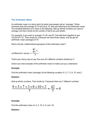
  • 1. The Arithmetic Mean An arithmetic mean is a fancy term for what most people call an "average." When someone says the average of 10 and 20 is 15, they are referring to the arithmetic mean. The simplest definition of a mean is the following: Add up all the numbers you want to average, and then divide by the number of items you just added. For example, if you want to average 10, 20, and 27, first add them together to get 10+20+27= 57. Then divide by 3 because we have three values, and we get an arithmetic mean (average) of 19. Want a formal, mathematical expression of the arithmetic mean? That's just a fancy way to say "the sum of k different numbers divided by k." Check out a few example of the arithmetic mean to make sure you understand: Example: Find the arithmetic mean (average) of the following numbers: 9, 3, 7, 3, 8, 10, and 2. Solution: Add up all the numbers. Then divide by 7 because there are 7 different numbers. Example: Find the arithmetic mean of -4, 3, 18, 0, 0, and -10. Solution:
  • 2. Sum the numbers. Divide by 6 because there are 6 numbers. The answer is 7/6, or 1.167 Geometric Mean The geometric mean is NOT the arithmetic mean and it is NOT a simple average. It is the nth root of the product of n numbers. That means you multiply a bunch of numbers together, and then take the nth root, where n is the number of values you just multiplied. Did that make sense? Here's a quick example: Example: What is the geometric mean of 2, 8 and 4? Solution: Multiply those numbers together. Then take the third root (cube root) because there are 3 numbers. Naturally, the geometric mean can get very complicated. Here's a mathematical definition of the geometric mean: Remember that the capital PI symbol means to multiply a series of numbers. That definition says to multiply k numbers and then take the kth root. One thing you should
  • 3. know is that the geometric mean only works with positive numbers. Negative numbers could result in imaginary results depending on how many negative numbers are in a set. Typically this isn't a problem, because most uses of the geometric mean involve real data, such as the length of physical objects or the number of people responding to a survey. Try a few more examples until you understand the geometric mean. Example: What is the geometric mean of 4, 9, 9, and 2? Solution: Just multiply the four numbers and take the 4th root: The geometric mean between two numbers is: The arithmetic mean between two numbers is: Example: The cut-off frequencies of a phone line are f1 = 300 Hz and f2 = 3300 Hz. What is the center frequency? The center frequency is f0 = 995 Hz as geometric mean and not f0 = 1800 Hz (arithmetic mean). What a difference! The geometric mean of two numbers is the square root of their product. The geometric mean of three numbers is the cubic root of their product. The arithmetic mean is the sum of the numbers, divided by the quantity of the numbers. Other names for arithmetic mean: average, mean, arithmetic average. In general, you can only take the geometric mean of positive numbers. The geometric mean, by definition, is the nth root of the product of the n units in a data
  • 4. set. For example, the geometric mean of 5, 7, 2, 1 is (5 × 7 × 2 × 1)1/4 = 2.893. Alternatively, if you log transform each of the individual units the geometric will be the exponential of the arithmetic mean of these log-transformed values. So, reusing the example above, exp [ ( ln(5) + ln(7) + ln(2) + ln(1) ) / 4 ] = 2.893. Geometric Mean Arithmetic Mean An arithmetic average is the sum of a series of numbers divided by the count of that series of numbers. If you were asked to find the class (arithmetic) average of test scores, you would simply add up all the test scores of the students, and then divide that sum by the number of students. For example, if five students took an exam and their scores were 60%, 70%, 80%, 90% and 100%, the arithmetic class average would be 80%. This would be calculated as: (0.6 + 0.7 + 0.8 + 0.9 + 1.0) / 5 = 0.8. The reason you use an arithmetic average for test scores is that each test score is an independent event. If one student happens to perform poorly on the exam, the next student's chances of doing poor (or well) on the exam isn't affected. In other words, each student's score is independent of the all other students' scores. However, there are some instances, particularly in the world of finance, where an arithmetic mean is not an appropriate method for calculating an average. Consider your investment returns, for example. Suppose you have invested your savings in the stock market for five years. If your returns each year were 90%, 10%, 20%, 30% and -90%, what would your average return be during this period? Well, taking the simple arithmetic average, you would get an answer of 12%. Not too shabby, you might think. However, when it comes to annual investment returns, the numbers are not
  • 5. independent of each other. If you lose a ton of money one year, you have that much less capital to generate returns during the following years, and vice versa. Because of this reality, we need to calculate the geometric average of your investment returns in order to get an accurate measurement of what your actual average annual return over the five-year period is. To do this, we simply add one to each number (to avoid any problems with negative percentages). Then, multiply all the numbers together, and raise their product to the power of one divided by the count of the numbers in the series. And you're finished - just don't forget to subtract one from the result! That's quite a mouthful, but on paper it's actually not that complex. Returning to our example, let's calculate the geometric average: Our returns were 90%, 10%, 20%, 30% and -90%, so we plug them into the formula as [(1.9 x 1.1 x 1.2 x 1.3 x 0.1) ^ 1/5] - 1. This equals a geometric average annual return of -20.08%. That's a heck of a lot worse than the 12% arithmetic average we calculated earlier, and unfortunately it's also the number that represents reality in this case. It may seem confusing as to why geometric average returns are more accurate than arithmetic average returns, but look at it this way: if you lose 100% of your capital in one year, you don't have any hope of making a return on it during the next year. In other words, investment returns are not independent of each other, so they require a geometric average to represent their mean.
  • 6. A matrix consists of a set of numbers arranged in rows and columns enclosed in brackets. The order of a matrix gives the number of rows followed by the number of columns in a matrix. The order of a matrix with 3 rows and 2 columns is 3 2 or 3 by 2. We usually denote a matrix by a capital letter. C is a matrix of order 2 × 4 (read as ‘2 by 4’) Elements In An Array Each number in the array is called an entry or an element of the matrix. When we need to read out the elements of an array, we read it out row by row.
  • 7. Each element is defined by its position in the matrix. In a matrix A, an element in row i and column j is represented by aij Example: a11 (read as ‘a one one ’)= 2 (first row, first column) a12 (read as ‘a one two') = 4 (first row, second column) a13 = 5, a21 = 7, a22 = 8, a23 = 9 Matrix Multiplication There are two matrix operations which we will use in our matrix transformations, multiplying (concatenating) two matrices, and transforming a vector by a matrix. We will now examine the first of these two operations, matrix multiplication. Matrix multiplication is the operation by which one matrix is transformed by another. A very important thing to remember is that matrix multiplication is not commutative. That is, [a] * [b] != [b] * [a]. For now, it will suffice to say that a matrix multiplication stores the results of the sum of the products of matrix rows and columns. Here is some example code of a matrix multiplication routine which multiplies matrix [a] * matrix [b], then copies the result to matrix a. void matmult(float a[4][4], float b[4][4])
  • 8. { float temp[4][4]; // temporary matrix for storing result int i, j; // row and column counters for (j = 0; j < 4; j++) // transform by columns first for (i = 0; i < 4; i++) // then by rows temp[i][j] = a[i][0] * b[0][j] + a[i][1] * b[1][j] + a[i][2] * b[2][j] + a[i][3] * b[3][j]; for (i = 0; i < 4; i++) // copy result matrix into matrix a for (j = 0; j < 4; j++) a[i][j] = temp[i][j]; } I have been informed that there is a faster way of multiplying matrices, which involves taking the dot product of rows and columns. However, I have yet to implement such a method, so I will not discuss it here at this time. Transforming a Vector by a Matrix This is the second operation which is required for our matrix transformations. It involves projecting a stationary vector onto transformed axis vectors using the dot product. One dot product is performed for each coordinate axis. x = x0 * matrix[0][0] + y0 * matrix[1][0] + z0 * matrix[2][0] + w0 * matrix[3][0]; y = x0 * matrix[0][1] + y0 * matrix[1][1] + z0 * matrix[2][1] + w0 * matrix[3][1]; z = x0 * matrix[0][2] + y0 * matrix[1][2] + z0 * matrix[2][2] + w0 * matrix[3][2]; The x0, y0, etc. coordinates are the original object space coordinates for the vector. That is, they never change due to transformation. "Alright," you say. "Where did all the w coordinates come from???" Good question :) The w coordinates come from what is known as a homogenous coordinate system, which is basically a way to represent 3d space in terms of a 4d matrix. Because we are limiting ourselves to 3d, we pick a constant, nonzero value for w (1.0 is a good choice, since anything * 1.0 = itself). If we use this identity axiom, we can eliminate a multiply from each of the dot products: x = x0 * matrix[0][0] + y0 * matrix[1][0] + z0 * matrix[2][0] + matrix[3][0]; y = x0 * matrix[0][1] + y0 * matrix[1][1] + z0 * matrix[2][1] + matrix[3][1];
  • 9. z = x0 * matrix[0][2] + y0 * matrix[1][2] + z0 * matrix[2][2] + matrix[3][2]; These are the formulas you should use to transform a vector by a matrix. Object Space Transformations Now that we know how to multiply matrices together, we can implement the actual formulas used in our transformations. There are three operations performed on a vector by a matrix transformation: translation, rotation, and scaling. Translation can best be described as linear change in position. This change can be represented by a delta vector [dx, dy, dz], where dx represents the change in the object's x position, dy represents the change in its y position, and dz its z position. If done correctly, object space translation allows objects to translate forward/backward, left/right, and up/down, relative to the current orientation of the object. Using our airplane as an example, if the nose of the airplane is oriented along the object's local z axis, then translating the airplane in the +z direction will make the airplane move forward (the direction in which its nose is pointing) regardless of the airplane's orientation. Here is the translation matrix: += =+ | += =+ += =+ += =+ += += | | | | | | | | | | | | | 1 | | 0 | | 0 | | 0 | | | | | | | | | | | | | | | | | | | | | | | | 0 | | 1 | | 0 | | 0 | | | | | | | | | | | | | | | | | | | | | | | | 0 | | 0 | | 1 | | 0 | | | += =+ += =+ += =+ | | | | +===============+ | | | | dy dx dz | 1 | | | +===============+ += =+ | += =+ where [dx, dy, dz] is the displacement vector. After this operation, the object will have moved in its own coordinate system, according to the displacement (translation) vector. The next operation that is performed by our matrix transformation is rotation. Rotation can be described as circular motion about some axis, in this case the axis is one of the object's local axes. Since there are three axes in each object, we need to rotate around each of them. Here are the matrices for rotation about each axis: about the x axis:
  • 10. += =+ | += =+ += =+ += =+ += += | | | | | | | | | | | | | 1 | | 0 | | 0 | | 0 | | | | | | | | | | | | | | | | | | | | | | | | 0 | |cx | |sx | | 0 | | | | | | | | | | | | | | | | | | | | | | | | 0 | |-sx| |cx | | 0 | | | += =+ += =+ += =+ | | | | +===============+ | | | | 0 0 0 | 1 | | | +===============+ += =+ | += =+ about the y axis: += =+ | += =+ += =+ += =+ += += | | | | | | | | | | | | |cy | | 0 | |-sy| | 0 | | | | | | | | | | | | | | | | | | | | | | | | 0 | | 1 | | 0 | | 0 | | | | | | | | | | | | | | | | | | | | | | | |sy | | 0 | |cy | | 0 | | | += =+ += =+ += =+ | | | | +===============+ | | | | 0 0 0 | 1 | | | +===============+ += =+ | += =+ about the z axis: += =+ | += =+ += =+ += =+ += += | | | | | | | | | | | | |cz | |sz | | 0 | | 0 | | | | | | | | | | | | | | | | | | | | | | | |-sz| |cz | | 0 | | 0 | | | | | | | | | | | | | | | | | | | | | | | | 0 | | 0 | | 1 | | 0 | | | += =+ += =+ += =+ | | | | +===============+ | | | | 0 0 0 | 1 | | | +===============+ += =+ | += =+
  • 11. The cx, sx, cy, sy, cz, and sz variables are the values of the cosines and sines of the angles of rotation about the x, y, and z axes, respectively. Remeber that the angles used represent angular displacement just as the values used in the translation step denote a linear displacement. Correct transformation CANNOT be accomplished with matrix multiplication if you use the cumulative angles of rotation. I have been told that quaternions are able to perform this operation correctly, however I know nothing of quaternions and how they are implemented. The incremental angles used here represent rotation from the current object orientation. In other words, by rotating 1 degree about the z axis, you are telling your object "Rotate 1 degree about your z axis, regardless of your current orientation, and regardless of how you got to that orientation." If you think about it a bit, you will realize that this is how the real world operates. In object space, the series of rotations an object undergoes to attain a certain orientation have no effect on the object space results of any upcoming rotations. Now that we know the matrix formulas for translation and rotation, we can combine them to transform our objects. The formula for transformations in object space is [O] = [O] * [T] * [X] * [Y] * [Z] where O is the object's matrix, T is the translation matrix, and X, Y, and Z are the rotation matrices for their respective axes. Remember, that order of matrix multiplication is very important! The recursive assignment of O poses a question: What is the original value of the object matrix? To eliminate any terrible errors in transformation, the matrices which store an object's orientation should always be initialized to identity. Matrix Multiplication You probably know what a matrix is already if you are interested in matrix multiplication. However, a quick example won't hurt. A matrix is just a two-dimensional group of numbers. Instead of a list, called a vector, a matrix is a rectangle, like the following: You can set a variable to be a matrix just as you can set a variable to be a number. In this case, x is the matrix containing those four numbers (in that particular order). Now, suppose you have two matrices that you need to multiply. Multiplication for numbers is pretty easy, but how do you do it for a matrix?
  • 12. Here is a key point: You cannot just multiply each number by the corresponding number in the other matrix. Matrix multiplication is not like addition or subtraction. It is more complicated, but the overall process is not hard to learn. Here's an example first, and then I'll explain what I did: Example: Solution: You're probably wondering how in the world I got that answer. Well you're justified in thinking that. Matrix multiplication is not an easy task to learn, and you do need to pay attention to avoid a careless error or two. Here's the process: • Step 1: Move across the top row of the first matrix, and down the first column of the second matrix:
  • 13. • Step 2: Multiply each number from the top row of the first matrix by the number in the first column on the second matrix. In this case, that means multiplying 1*2 and 6*9. Then, take the sum of those values (2+54): • Step 3: Insert the value you just got into the answer matrix. Since we are multiplying the 1st row and the 1st column, our answer goes into that slot in the answer matrix: • Step 4: Repeat for the other rows and columns. That means you need to walk down the first row of the first matrix and this time the second column of the second matrix. Then the second row of the first matrix and the first column of the second, and finally the bottom of the first matrix and the right column of the second matrix:
  • 14. • Step 5: Insert all of those values into the answer matrix. I just showed you how to do top left and the bottom right. If you work the other two numbers, you will get 1*2+6*7=44 and 3*2+8*9=78. Insert them into the answer matrix in the corresponding positions and you get: Now I know what you're thinking. That was really hard!!! Well it will seem that way until you get used to the process. It may help you to write out all your work, and even draw arrows to remember which way you're moving in the rows and columns. Just remember to multiply each row in the first matrix by each column in the second matrix. What if the matrices aren't squares? Then you have to add another step. In order to multiply two matrices, the matrix on the left must have as many columns as the matrix
  • 15. on the right has rows. That way you can match up each pair while you're multiplying. The size of the final matrix is determined by the rows in the left matrix and the columns in the right. Here's what I do: I write down the sizes of the matrices. The left matrix has 2 rows and 3 columns, so that's how we write it. Rows, columns, in that order. The other matrix is a 3x1 matrix because it has 3 rows and just 1 column. If the numbers in the middle match up you can multiply. The outside numbers give you the size of the answer. Even if you mess this up you'll figure it out eventually because you won't be able to multiply. Here's an important reminder: Matrix Multiplication is not commutative. That means you cannot switch the order and expect the same result! Regular multiplication tells us that 4*3=3*4, but this is not multiplication of the usual sense. Finally, here's an example with uneven matrix sizes to wrap things up: Example:
  • 16. Lab 1: Matrix Calculation Examples Given the Following Matrices: A= 1.00 2.00 3.00 4.00 5.00 6.00 7.00 8.00 9.00
  • 17. B= 1.00 1.00 1.00 2.00 2.00 2.00 C= 1.00 2.00 1.00 3.00 2.00 2.00 1.00 5.00 3.00 1) Calculate A + C 2) Calculate A - C 3) Calculate A * C (A times C) 4) Calculate B * A (B time A) 5) Calculate A .* C (A element by element multiplication with C) 6) Inverse of C
  • 18. Matrix Calculation Examples - Answers A + C= 2.00 4.00 4.00 7.00 7.00 8.00 8.00 13.00 12.00 A - C= 0.00 0.00 2.00 1.00 3.00 4.00 6.00 3.00 6.00 A * C= 10.00 21.00 14.00 25.00 48.00 32.00 40.00 75.00 50.00 B * A= 12.00 15.00 18.00
  • 19. 24.00 30.00 36.00 Element by element multiplication A .* C= 1.00 4.00 3.00 12.00 10.00 12.00 7.00 40.00 27.00 Inverse of C= 0.80 0.20 -0.40 1.40 -0.40 -0.20 -2.60 0.60 0.80
  • 20. Matrix Calculation Assignment Given the Following Matrices: A= 1.00 2.00 3.00 6.00 5.00 4.00 9.00 8.00 7.00 B= 2.00 2.00 2.00 3.00 3.00 3.00 C= 1.00 2.00 1.00 4.00 3.00 1.00 3.00 4.00 2.00
  • 21. 1) Calculate A + C 2) Calculate A - C 3) Calculate A * C (A times C) 4) Calculate B * A (B time A) 5) Calculate A .* C (A element by element multiplication with C) Vector product VS dot product in matrix hi, i don't really understand whats the difference between vector product and dot product in matrix form. for example (1 2) X (1 2) (3 4) (3 4) = ? so when i take rows multiply by columns, to get a 2x2 matrix, i am doing vector product? so what then is dot producT? lastly, my notes says |detT| = final area of basic box/ initial area of basic box where detT = (Ti) x (Tj) . (Tk) so, whats the difference between how i should work out x VS . ? also, |detT| = magnitude of T right? so is there a formula i should use to find magnitude? so why is |k . k| = 1? thanks PhysOrg.com science news on PhysOrg.com >> Smooth-talking hackers test hi-tech titans' skills >> Reading terrorists minds about imminent attack: P300 brain waves correlated to guilty knowledge >> Nano 'pin art': NIST arrays are step toward mass production of nanowires Apr25-10, 07:35 AM Last edited by HallsofIvy; Apr27-10 at 07:42 AM.. #2 HallsofIvy HallsofIvy is Offline: Posts: 26,845 Re: Vector product VS dot product in matrix Originally Posted by quietrain hi, i don't really understand whats the difference between vector product and dot product in matrix form. for example
  • 22. (1 2) X (1 2) (3 4) (3 4) = ? so when i take rows multiply by columns, to get a 2x2 matrix, i am doing vector product? No, you are doing a "matrix product". There are no vectors here. so what then is dot producT? With matrices? It isn't anything. The matrix product is the only multiplication defined for matrices. The dot product is defined for vectors, not matrices. lastly, my notes says |detT| = final area of basic box/ initial area of basic box where detT = (Ti) x (Tj) . (Tk) Well, we don't have your notes so we have no idea what "T", "Ti", "Tj", "Tk" are nor do we know what a "basic box" is. I do know that if you have a "parallelpiped" with adjacent sides given by the vectors , , and , then the volume (not area) of the parallelpiped is given by the "triple product", which can be represented by determinant having the components of the vectors as rows. That has nothing at all to do with matrices. so, whats the difference between how i should work out x VS . ? also, |detT| = magnitude of T right? No, "det" applies only to square arrays for which "magnitude" is not defined. so is there a formula i should use to find magnitude? so why is |k . k| = 1? thanks I guess you mean "k" to be the unit vector in the z direction in a three dimensional coordinate system. If so, then |k.k| is, by definition, the length of k which is, again by definition of "unit vector", 1. You seem to be confusing a number of very different concepts. Go back and review. Apr27-10, 01:02 AM #3
  • 23. quietrain quietrain is Offline: Posts: 173 Re: Vector product VS dot product in matrix oh.. em.. ok lets say we have (1 2) x (4 5) (3 4) (6 7) = so this is just rows multiply by column to get a 2x2 matrix right? so what is the difference if i replace the x sign with the dot sign now. do i still get the same? i presume one is cross (x) product , one is dot (.) product? or is it for matrix there is no such things as cross or dot product? thats weird. my tutor tells us to know the difference between cross and dot matrix product so for the case of the parallelpiped, whats the significance of the triple product (u x v) .w? why do we use x for u&v but . for w? is it just to tell us that we have to use sin and cos respectively? but if u v and w were square matrix, then there won't be any sin and cos to use? so we just multiply as usual rows by columns? oh by definition . so that means |k.k| = (k)(k)cos(0) = (1)(1)cos(0) = 1 so |i.k| = (1)(1)cos(90) = 0 ? so if i x k gives us -j by the right hand rule, then does it mean the magnitude, which is |i.k| = 0 is 0? in the direction of the -j?? or are they 2 totally different aspects? btw, sry for another question, why is e(w)(A) , where A = (0 -1) (1 0) can be expressed as ( cosw -sinw) ( sinw cosw) which is the rotational matrix anti-clockwise about the x-axis right? thanks Apr27-10, 08:08 AM Last edited by HallsofIvy; Apr27-10 at 08:16 AM.. #4 HallsofIvy HallsofIvy is Offline: Posts: 26,845 Re: Vector product VS dot product in matrix Originally Posted by quietrain oh.. em.. ok lets say we have (1 2) x (4 5) (3 4) (6 7) = so this is just rows multiply by column to get a 2x2 matrix right? so what is the difference if i replace the x sign with the dot sign now. do i still get the same? You can replace it by whatever symbol you like. As long as your multiplication is "matrix multiplication" you will get the same result.
  • 24. i presume one is cross (x) product , one is dot (.) product? No, just changing the symbol doesn't make it one or the other. or is it for matrix there is no such things as cross or dot product? thats weird. my tutor tells us to know the difference between cross and dot matrix product I suspect your tutor was talking about vectors not matrices. so for the case of the parallelpiped, whats the significance of the triple product (u x v) .w? why do we use x for u&v but . for w? Because you are talking about vectors not matrices! is it just to tell us that we have to use sin and cos respectively? but if u v and w were square matrix, then there won't be any sin and cos to use? so we just multiply as usual rows by columns? They are NOT matrices, they are vectors!! You can think of vectors as "row matrices" (n by 1) or "column matrices" (1 by n) but they still have properties that matrices in general do not have. oh by definition . so that means |k.k| = (k)(k)cos(0) = (1)(1)cos(0) = 1 so |i.k| =(1)(1)cos(90) = 0 ? Yes, that is correct. so if i x k gives us -j by the right hand rule, then does it mean the magnitude, which is |i.k| = 0 is 0? in the direction of the -j?? or are they 2 totally different aspects? No, the length of i x k is NOT |i.k|, it is . In general, the length of is where is the angle between and . btw, sry for another question, why is e(w)(A) , where A = (0 -1) (1 0) can be expressed as ( cosw -sinw) ( sinw cosw) which is the rotational matrix anti-clockwise about the x-axis right? thanks For objects other than numbers, where we have a notion of addition and multiplication, we define higher functions by using their "Taylor series", power series that are equal to the functions. In
  • 25. particular, . It should be easy to calculate that and, since that is the identity matrix, it all repeats: etc. That gives and you should be able to recognise those as the Taylor's series about 0 for cos(w) and sin(w). Apr27-10, 09:15 AM #5 quietrain quietrain is Offline: Posts: 173 Re: Vector product VS dot product in matrix wow. ok, i went to check again what my tutor said and it was "scalar and vector products in terms of matrices". so what does he mean by this? the scalar product is (A B C) x (D E F)T , (so we can take the transpose of DEF because it is symmetric matrix? or is it for some other reason? ) so rows multiply by columns again? but what about vector product? for the parallelpiped, (u x v).w so lets say u = (1,1) , v = (2,2), w = (3,3) so u x v = (1x2, 1x2)sin(angle between vectors) so .w = (2x3,2x3) cos(angle) ? so if it yields 0, that vector w lies in the plane define by u and v, but if its otherwise, then w doesn't lie in the plane of u v ? for i x k, why is the length |i||j|? why is j introduced here? shouldn't it be |i||k|sin(90) = 1?
  • 26. oh i see.. so the right hand rule gives the direection but the magnitude for i x k = |i||k|sin(90) = 1? thanks a ton! Apr27-10, 11:40 AM #6 HallsofIvy HallsofIvy is Offline: Posts: 26,845 Re: Vector product VS dot product in matrix Originally Posted by quietrain wow. ok, i went to check again what my tutor said and it was "scalar and vector products in terms of matrices". so what does he mean by this? the scalar product is (A B C) x (D E F)T , (so we can take the transpose of DEF because it is symmetric matrix? or is it for some other reason? ) so rows multiply by columns again? Okay, you think of one vector as a row matrix and the other as a column matrix then the "dot product" is the matrix product But the dot product is commutative isn't it? Does it really make sense to treat the two vectors as different kinds of matrices? It is really better here to think of this not as the product of two vectors but a vector in a vector space and functional in the dual space. but what about vector product for the parallelpiped, (u x v).w so lets say u = (1,1) , v = (2,2), w = (3,3) so u x v = (1x2, 1x2)sin(angle between vectors) so .w = (2x3,2x3) cos(angle) ? so if it yields 0, that vector w lies in the plane define by u and v, but if its otherwise, then w doesn't lie in the plane of u v ? for i x k, why is the length |i||j|? why is j introduced here? shouldn't it be |i||k|sin(90) = 1? Yes, that was a typo. I meant |i||k|. oh i see.. so the right hand rule gives the direection but the magnitude for i x k = |i||k|sin(90) = 1? Yes. thanks a ton!
  • 27. Matrix (mathematics) From Wikipedia, the free encyclopedia Specific entries of a matrix are often referenced by using pairs of subscripts. In mathematics, a matrix (plural matrices, or less commonly matrixes) is a rectangular array of numbers, such as
  • 28. An item in a matrix is called an entry or an element. The example has entries 1, 9, 13, 20, 55, and 4. Entries are often denoted by a variable with twosubscripts, as shown on the right. Matrices of the same size can be added and subtracted entrywise and matrices of compatible sizes can be multiplied. These operations have many of the properties of ordinary arithmetic, except that matrix multiplication is not commutative, that is, AB and BA are not equal in general. Matrices consisting of only one column or row define the components of vectors, while higher-dimensional (e.g., three-dimensional) arrays of numbers define the components of a generalization of a vector called a tensor. Matrices with entries in other fields or rings are also studied. Matrices are a key tool in linear algebra. One use of matrices is to represent linear transformations, which are higher-dimensional analogs of linear functions of the form f(x) = cx, where c is a constant; matrix multiplication corresponds to composition of linear transformations. Matrices can also keep track of thecoefficients in a system of linear equations. For a square matrix, the determinant and inverse matrix (when it exists) govern the behavior of solutions to the corresponding system of linear equations, and eigenvalues and eigenvectors provide insight into the geometry of the associated linear transformation. Matrices find many applications. Physics makes use of matrices in various domains, for example in geometrical optics and matrix mechanics; the latter led to studying in more detail matrices with an infinite number of rows and columns. Graph theory uses matrices to keep track of distances between pairs of vertices in a graph. Computer graphics uses matrices to project 3- dimensional space onto a 2-dimensional screen. Matrix calculus generalizes classical analytical notions such as derivatives of functions or exponentials to matrices. The latter is a recurring need in solving ordinary differential equations.Serialism and dodecaphonism are musical movements of the 20th century that use a square mathematical matrix to determine the pattern of music intervals. A major branch of numerical analysis is devoted to the development of efficient algorithms for matrix computations, a subject that is centuries old but still an active area of research. Matrix decomposition methods simplify computations, both theoretically and practically. For sparse matrices, specifically tailored
  • 29. algorithms can provide speedups; such matrices arise in the finite element method, for example. Definition A matrix is a rectangular arrangement of numbers.[1] For example, An alternative notation uses large parentheses instead of box brackets: The horizontal and vertical lines in a matrix are called rows and columns, respectively. The numbers in the matrix are called its entries or its elements. To specify a matrix's size, a matrix with m rows and ncolumns is called an m-by-n matrix or m × n matrix, while m and n are called its dimensions. The above is a 4-by-3 matrix. A matrix with one row (a 1 × n matrix) is called a row vector, and a matrix with one column (an m × 1 matrix) is called a column vector. Any row or column of a matrix determines a row or column vector, obtained by removing all other rows respectively columns from the matrix. For example, the row vector for the third row of the above matrix A is When a row or column of a matrix is interpreted as a value, this refers to the corresponding row or column vector. For instance one may say that two different rows of a matrix are equal, meaning they determine the same row vector. In some cases the value of a row or column should be interpreted just as a sequence of values (an element of Rn if entries are real numbers) rather than as a matrix, for instance when saying that the rows of a matrix are equal to the corresponding columns of its transpose matrix. Most of this article focuses on real and complex matrices, i.e., matrices whose entries are real or complex numbers. More general types of entries are discussed below.
  • 30. [edit]Notation The specifics of matrices notation varies widely, with some prevailing trends. Matrices are usually denoted using upper-case letters, while the corresponding lower-case letters, with two subscript indices, represent the entries. In addition to using upper-case letters to symbolize matrices, many authors use a special typographical style, commonly boldface upright (non-italic), to further distinguish matrices from other variables. An alternative notation involves the use of a double-underline with the variable name, with or without boldface style, (e.g., ). The entry that lies in the i-th row and the j-th column of a matrix is typically referred to as the i,j, (i,j), or (i,j)th entry of the matrix. For example, the (2,3) entry of the above matrix A is 7. The (i, j)th entry of a matrix A is most commonly written as ai,j. Alternative notations for that entry are A[i,j] or Ai,j. Sometimes a matrix is referred to by giving a formula for its (i,j)th entry, often with double parenthesis around the formula for the entry, for example, if the (i,j)th entry of A were given by aij, A would be denoted ((aij)). An asterisk is commonly used to refer to whole rows or columns in a matrix. For example, ai, ∗ refers to the ith row of A, and a ∗ ,j refers to the jth column of A. The set of all m-by-n matrices is denoted (m,n). A common shorthand is A = [ai,j]i=1,...,m; j=1,...,n or more briefly A = [ai,j]m×n to define an m × n matrix A. Usually the entries ai,j are defined separately for all integers 1 ≤ i ≤ m and 1 ≤ j ≤ n. They can however sometimes be given by one formula; for example the 3-by-4 matrix can alternatively be specified by A = [i − j]i=1,2,3; j=1,...,4, or simply A = ((i-j)), where the size of the matrix is understood. Some programming languages start the numbering of rows and columns at zero, in which case the entries of an m-by-n matrix are indexed by 0 ≤ i ≤ m − 1 and 0 ≤ j ≤ n − 1.[2] This article follows the more common convention in mathematical writing where enumeration starts from 1.
  • 31. [edit]Basic operations Main articles: Matrix addition, Scalar multiplication, Transpose, and Row operations There are a number of operations that can be applied to modify matrices called matrix addition, scalar multiplication and transposition.[3] These form the basic techniques to deal with matrices. Operation Definition Example Addition The sum A+B of two m- by-n matrices A and B is calculated entrywise: (A + B)i,j = Ai,j + Bi ,j, where 1 ≤ i ≤ m and 1 ≤ j ≤ n. Scalar multiplicati on The scalar multiplication cA of a matrix A and a number c (also called a scalar in the parlance ofabstract algebra) is given by multiplying every entry of A by c: (cA)i,j = c · Ai,j. Transp ose The transpose of an m-by- n matrix A is the n-by-m m atrix AT (also denoted Atr or t A) formed by turning rows into columns and vice versa:
  • 32. (AT )i,j = Aj,i. Familiar properties of numbers extend to these operations of matrices: for example, addition is commutative, i.e. the matrix sum does not depend on the order of the summands: A + B = B + A.[4] The transpose is compatible with addition and scalar multiplication, as expressed by (cA)T = c(AT ) and (A + B)T = AT + BT . Finally, (AT )T = A. Row operations are ways to change matrices. There are three types of row operations: row switching, that is interchanging two rows of a matrix, row multiplication, multiplying all entries of a row by a non-zero constant and finally row addition which means adding a multiple of a row to another row. These row operations are used in a number of ways including solving linear equations and finding inverses. [edit]Matrix multiplication, linear equations and linear transformations Main article: Matrix multiplication Schematic depiction of the matrix product AB of two matrices A and B. Multiplication of two matrices is defined only if the number of columns of the left matrix is the same as the number of rows of the right matrix. If A is an m-by-n matrix and B is an n-by-p matrix, then their matrix product AB is the m-by-p matrix whose entries are given by dot-product of the corresponding row of A and the corresponding column of B: where 1 ≤ i ≤ m and 1 ≤ j ≤ p.[5] For example (the underlined entry 1 in the product is calculated as the product 1 · 1 + 0 · 1 + 2 · 0 = 1):
  • 33. Matrix multiplication satisfies the rules (AB)C = A(BC) (associativity), and (A+B)C = AC+BC as well as C(A+B) = CA+CB (left and right distributivity), whenever the size of the matrices is such that the various products are defined. [6] The product AB may be defined without BA being defined, namely if A and B are m-by-n and n-by-k matrices, respectively, and m ≠ k. Even if both products are defined, they need not be equal, i.e. generally one has AB ≠ BA, i.e., matrix multiplication is not commutative, in marked contrast to (rational, real, or complex) numbers whose product is independent of the order of the factors. An example of two matrices not commuting with each other is: whereas The identity matrix In of size n is the n-by-n matrix in which all the elements on the main diagonal are equal to 1 and all other elements are equal to 0, e.g. It is called identity matrix because multiplication with it leaves a matrix unchanged: MIn = ImM = M for any m-by-n matrix M. Besides the ordinary matrix multiplication just described, there exist other less frequently used operations on matrices that can be considered forms of multiplication, such as the Hadamard product and theKronecker product.[7] They arise in solving matrix equations such as the Sylvester equation. [edit]Linear equations Main articles: Linear equation and System of linear equations A particular case of matrix multiplication is tightly linked to linear equations: if x designates a column vector (i.e. n×1-matrix) of n variables x1, x2, ..., xn, and A is an m-by-n matrix, then the matrix equation
  • 34. Ax = b, where b is some m×1-column vector, is equivalent to the system of linear equations A1,1x1 + A1,2x2 + ... + A1,nxn = b1 ... Am,1x1 + Am,2x2 + ... + Am,nxn = bm .[8] This way, matrices can be used to compactly write and deal with multiple linear equations, i.e. systems of linear equations. [edit]Linear transformations Main articles: Linear transformation and Transformation matrix Matrices and matrix multiplication reveal their essential features when related to linear transformations, also known as linear maps. A real m-by-n matrix A gives rise to a linear transformation Rn → Rm mapping each vector x in Rn to the (matrix) product Ax, which is a vector in Rm . Conversely, each linear transformation f: Rn → Rm arises from a unique m-by-n matrix A: explicitly, the (i, j)- entry of A is theith coordinate of f(ej), where ej = (0,...,0,1,0,...,0) is the unit vector with 1 in the jth position and 0 elsewhere. The matrix A is said to represent the linear map f, and A is called the transformation matrix of f. The following table shows a number of 2-by-2 matrices with the associated linear maps of R2 . The blue original is mapped to the green grid and shapes, the origin (0,0) is marked with a black point. Vertical shear with m=1.25. Horizontal flip Squeeze mapping with r=3/2 Scaling by a factor of 3/2 Rotation by π/6R = 30°
  • 35. Under the 1-to-1 correspondence between matrices and linear maps, matrix multiplication corresponds to composition of maps:[9] if a k-by-m matrix B represents another linear map g : Rm → Rk , then the composition g ∘ f is represented by BA since (g ∘ f)(x) = g(f(x)) = g(Ax) = B(Ax) = (BA)x. The last equality follows from the above-mentioned associativity of matrix multiplication. The rank of a matrix A is the maximum number of linearly independent row vectors of the matrix, which is the same as the maximum number of linearly independent column vectors.[10] Equivalently it is thedimension of the image of the linear map represented by A.[11] The rank-nullity theorem states that the dimension of the kernel of a matrix plus the rank equals the number of columns of the matrix.[12] Square matrices A square matrix is a matrix which has the same number of rows and columns. An n- by-n matrix is known as a square matrix of order n. Any two square matrices of the same order can be added and multiplied. A square matrix A is called invertible or non-singular if there exists a matrix B such that AB = In.[13] This is equivalent to BA = In.[14] Moreover, if B exists, it is unique and is called the inverse matrix of A, denoted A−1 . The entries Ai,i form the main diagonal of a matrix. The trace, tr(A) of a square matrix A is the sum of its diagonal entries. While, as mentioned above, matrix multiplication is not commutative, the trace of the product of two matrices is independent of the order of the factors: tr(AB) = tr(BA).[15] If all entries outside the main diagonal are zero, A is called a diagonal matrix. If only all entries above (below) the main diagonal are zero, A is called a lower triangular matrix (upper triangular matrix, respectively). For example, if n = 3, they look like
  • 36. (diagonal), (lower) and (upper triangular matrix). [edit]Determinant Main article: Determinant A linear transformation on R2 given by the indicated matrix. The determinant of this matrix is −1, as the area of the green parallelogram at the right is 1, but the map reverses theorientation, since it turns the counterclockwise orientation of the vectors to a clockwise one. The determinant det(A) or |A| of a square matrix A is a number encoding certain properties of the matrix. A matrix is invertible if and only if its determinant is nonzero. Its absolute value equals the area (in R2 ) or volume (in R3 ) of the image of the unit square (or cube), while its sign corresponds to the orientation of the corresponding linear map: the determinant is positive if and only if the orientation is preserved. The determinant of 2-by-2 matrices is given by the determinant of 3-by-3 matrices involves 6 terms (rule of Sarrus). The more lengthy Leibniz formula generalises these two formulae to all dimensions.[16] The determinant of a product of square matrices equals the product of their determinants: det(AB) = det(A) · det(B).[17] Adding a multiple of any row to another row, or a multiple of any column to another column, does not change the determinant. Interchanging two rows or two columns affects the determinant by multiplying it by −1.[18] Using these operations, any matrix can be transformed to a lower (or upper) triangular matrix, and for such matrices the determinant equals the
  • 37. product of the entries on the main diagonal; this provides a method to calculate the determinant of any matrix. Finally, the Laplace expansion expresses the determinant in terms of minors, i.e., determinants of smaller matrices.[19] This expansion can be used for a recursive definition of determinants (taking as starting case the determinant of a 1-by-1 matrix, which is its unique entry, or even the determinant of a 0-by-0 matrix, which is 1), that can be seen to be equivalent to the Leibniz formula. Determinants can be used to solve linear systems using Cramer's rule, where the division of the determinants of two related square matrices equates to the value of each of the system's variables.[20] [edit]Eigenvalues and eigenvectors Main article: Eigenvalues and eigenvectors A number λ and a non-zero vector v satisfying Av = λv are called an eigenvalue and an eigenvector of A, respectively.[nb 1][21] The number λ is an eigenvalue of an n×n-matrix A if and only if A−λIn is not invertible, which is equivalent to [22] The function pA(t) = det(A−tI) is called the characteristic polynomial of A, its degree is n. Therefore pA(t) has at most n different roots, i.e., eigenvalues of the matrix.[23] They may be complex even if the entries of A are real. According to the Cayley-Hamilton theorem, pA(A) = 0, that is to say, the characteristic polynomial applied to the matrix itself yields the zero matrix. [edit]Symmetry A square matrix A that is equal to its transpose, i.e. A = AT , is a symmetric matrix; if it is equal to the negative of its transpose, i.e. A = −AT , then it is a skew-symmetric matrix. In complex matrices, symmetry is often replaced by the concept of Hermitian matrices, which satisfy A ∗ = A, where the star or asterisk denotes the conjugate transpose of the matrix, i.e. the transpose of the complex conjugateof A. By the spectral theorem, real symmetric matrices and complex Hermitian matrices have an eigenbasis; i.e., every vector is expressible as a linear combination of eigenvectors. In both cases, all eigenvalues are real.[24] This theorem can be generalized to infinite-dimensional situations related to matrices with infinitely many rows and columns, see below.
  • 38. [edit]Definiteness Matrix A; definiteness; associated quadratic form QA(x,y); set of vectors (x,y) such that QA(x,y)=1 positive definite indefinite 1/4 x2 + y2 1/4 x2 − 1/4 y2 Ellipse Hyperbola A symmetric n×n-matrix is called positive-definite (respectively negative-definite; indefinite), if for all nonzero vectors x ∈ Rn the associatedquadratic form given by Q(x) = xT Ax takes only positive values (respectively only negative values; both some negative and some positive values).[25] If the quadratic form takes only non-negative (respectively only non-positive) values, the symmetric matrix is called positive- semidefinite (respectively negative-semidefinite); hence the matrix is indefinite precisely when it is neither positive-semidefinite nor negative-semidefinite. A symmetric matrix is positive-definite if and only if all its eigenvalues are positive. [26] The table at the right shows two possibilities for 2-by-2 matrices. Allowing as input two different vectors instead yields the bilinear form associated to A: BA (x, y) = xT Ay.[27] [edit]Computational aspects In addition to theoretical knowledge of properties of matrices and their relation to other fields, it is important for practical purposes to perform matrix calculations effectively and precisely. The domain studying these matters is called numerical linear algebra.[28] As with other numerical situations, two main aspects are
  • 39. the complexity of algorithms and theirnumerical stability. Many problems can be solved by both direct algorithms or iterative approaches. For example, finding eigenvectors can be done by finding a sequence of vectors xn converging to an eigenvector when n tends to infinity.[29] Determining the complexity of an algorithm means finding upper bounds or estimates of how many elementary operations such as additions and multiplications of scalars are necessary to perform some algorithm, e.g. multiplication of matrices. For example, calculating the matrix product of two n-by-n matrix using the definition given above needs n3 multiplications, since for any of the n2 entries of the product, n multiplications are necessary. The Strassen algorithm outperforms this "naive" algorithm; it needs only n2.807 multiplications.[30] A refined approach also incorporates specific features of the computing devices. In many practical situations additional information about the matrices involved is known. An important case are sparse matrices, i.e. matrices most of whose entries are zero. There are specifically adapted algorithms for, say, solving linear systems Ax = b for sparse matrices A, such as the conjugate gradient method.[31] An algorithm is, roughly speaking, numerical stable, if little deviations (such as rounding errors) do not lead to big deviations in the result. For example, calculating the inverse of a matrix via Laplace's formula(Adj (A) denotes the adjugate matrix of A) A−1 = Adj(A) / det(A) may lead to significant rounding errors if the determinant of the matrix is very small. The norm of a matrix can be used to capture the conditioning of linear algebraic problems, such as computing a matrix' inverse.[32] Although most computer languages are not designed with commands or libraries for matrices, as early as the 1970s, some engineering desktop computers such as the HP 9830 had ROM cartridges to add BASIC commands for matrices. Some computer languages such as APL were designed to manipulate matrices, and various mathematical programs can be used to aid computing with matrices.[33] [edit]Matrix decomposition methods Main articles: Matrix decomposition, Matrix diagonalization, and Gaussian elimination There are several methods to render matrices into a more easily accessible form. They are generally referred to as matrix transformation or matrix
  • 40. decomposition techniques. The interest of all these decomposition techniques is that they preserve certain properties of the matrices in question, such as determinant, rank or inverse, so that these quantities can be calculated after applying the transformation, or that certain matrix operations are algorithmically easier to carry out for some types of matrices. The LU decomposition factors matrices as a product of lower (L) and an upper triangular matrices (U).[34] Once this decomposition is calculated, linear systems can be solved more efficiently, by a simple technique called forward and back substitution. Likewise, inverses of triangular matrices are algorithmically easier to calculate. The Gaussian elimination is a similar algorithm; it transforms any matrix to row echelon form.[35] Both methods proceed by multiplying the matrix by suitable elementary matrices, which correspond to permuting rows or columns and adding multiples of one row to another row. Singular value decomposition expresses any matrix A as a product UDV ∗ , where U and V are unitary matrices and D is a diagonal matrix. A matrix in Jordan normal form. The grey blocks are called Jordan blocks. The eigendecomposition or diagonalization expresses A as a product VDV−1 , where D is a diagonal matrix and V is a suitable invertible matrix.[36] If A can be written in this form, it is called diagonalizable. More generally, and applicable to all matrices, the Jordan decomposition transforms a matrix into Jordan normal form, that is to say matrices whose only nonzero entries are the eigenvalues λ1 to λn of A, placed on the main diagonal and possibly entries equal to one directly above the main diagonal, as shown at the right.[37] Given the eigendecomposition, the nth power of A (i.e. n-fold iterated matrix multiplication) can be calculated via An = (VDV−1 )n = VDV−1 VDV−1 ...VDV−1 = VDn V−1
  • 41. and the power of a diagonal matrix can be calculated by taking the corresponding powers of the diagonal entries, which is much easier than doing the exponentiation for Ainstead. This can be used to compute the matrix exponential eA , a need frequently arising in solving linear differential equations, matrix logarithms and square roots of matrices.[38] To avoid numerically ill- conditioned situations, further algorithms such as the Schur decomposition can be employed.[39] [edit]Abstract algebraic aspects and generalizations Matrices can be generalized in different ways. Abstract algebra uses matrices with entries in more general fields or even rings, while linear algebra codifies properties of matrices in the notion of linear maps. It is possible to consider matrices with infinitely many columns and rows. Another extension are tensors, which can be seen as higher-dimensional arrays of numbers, as opposed to vectors, which can often be realised as sequences of numbers, while matrices are rectangular or two- dimensional array of numbers.[40] Matrices, subject to certain requirements tend to form groups known as matrix groups. [edit]Matrices with more general entries This article focuses on matrices whose entries are real or complex numbers. However, matrices can be considered with much more general types of entries than real or complex numbers. As a first step of generalization, any field, i.e. a set where addition, subtraction, multiplication and division operations are defined and well-behaved, may be used instead of R or C, for example rational numbers or finite fields. For example, coding theory makes use of matrices over finite fields. Wherever eigenvalues are considered, as these are roots of a polynomial they may exist only in a larger field than that of the coefficients of the matrix; for instance they may be complex in case of a matrix with real entries. The possibility to reinterpret the entries of a matrix as elements of a larger field (e.g., to view a real matrix as a complex matrix whose entries happen to be all real) then allows considering each square matrix to possess a full set of eigenvalues. Alternatively one can consider only matrices with entries in an algebraically closed field, such as C, from the outset. More generally, abstract algebra makes great use of matrices with entries in a ring R.[41] Rings are a more general notion than fields in that no division operation exists. The very same addition and multiplication operations of matrices extend to this setting, too. The set M(n, R) of all square n-by-n matrices over R is a ring called matrix ring, isomorphic to the endomorphism ring of the left R-moduleRn .[42] If
  • 42. the ring R is commutative, i.e., its multiplication is commutative, then M(n, R) is a unitary noncommutative (unless n = 1) associative algebra over R. The determinant of square matrices over a commutative ring R can still be defined using the Leibniz formula; such a matrix is invertible if and only if its determinant is invertible in R, generalising the situation over a field F, where every nonzero element is invertible.[43] Matrices over superrings are called supermatrices.[44] Matrices do not always have all their entries in the same ring - or even in any ring at all. One special but common case is block matrices, which may be considered as matrices whose entries themselves are matrices. The entries need not be quadratic matrices, and thus need not be members of any ordinary ring; but their sizes must fulfil certain compatibility conditions. [edit]Relationship to linear maps Linear maps Rn → Rm are equivalent to m-by-n matrices, as described above. More generally, any linear map f: V → W between finite-dimensional vector spaces can be described by a matrix A = (aij), after choosing bases v1, ..., vn of V, and w1, ..., wm of W (so n is the dimension of V and m is the dimension of W), which is such that In other words, column j of A expresses the image of vj in terms of the basis vectors wi of W; thus this relationuniquely determines the entries of the matrix A. Note that the matrix depends on the choice of the bases: different choices of bases give rise to different, but equivalent matrices.[45] Many of the above concrete notions can be reinterpreted in this light, for example, the transpose matrix AT describes thetranspose of the linear map given by A, with respect to the dual bases.[46] Graph theory
  • 43. An undirected graph with adjacency matrix The adjacency matrix of a finite graph is a basic notion of graph theory.[62] It saves which vertices of the graph are connected by an edge. Matrices containing just two different values (0 and 1 meaning for example "yes" and "no") are called logical matrices. The distance (or cost) matrix contains information about distances of the edges.[63] These concepts can be applied to websites connected hyperlinks or cities connected by roads etc., in which case (unless the road network is extremely dense) the matrices tend to be sparse, i.e. contain few nonzero entries. Therefore, specifically tailored matrix algorithms can be used in network theory. [edit]Analysis and geometry The Hessian matrix of a differentiable function ƒ: Rn → R consists of the second derivatives of ƒ with respect to the several coordinate directions, i.e.[64] It encodes information about the local growth behaviour of the function: given a critical point x = (x1, ..., xn), i.e., a point where the first partial derivatives of ƒ vanish, the function has a local minimum if the Hessian matrix is positive definite. Quadratic programming can be used to find global minima or maxima of quadratic functions closely related to the ones attached to matrices (see above).[65] At the saddle point (x = 0, y = 0) (red) of the function f(x,−y) = x2 − y2 , the Hessian matrix is indefinite.
  • 44. Another matrix frequently used in geometrical situations is the Jacobi matrix of a differentiable map f: Rn → Rm . If f1, ..., fm denote the components of f, then the Jacobi matrix is defined as [66] If n > m, and if the rank of the Jacobi matrix attains its maximal value m, f is locally invertible at that point, by the implicit function theorem.[67] Partial differential equations can be classified by considering the matrix of coefficients of the highest-order differential operators of the equation. For elliptic partial differential equations this matrix is positive definite, which has decisive influence on the set of possible solutions of the equation in question.[68] The finite element method is an important numerical method to solve partial differential equations, widely applied in simulating complex physical systems. It attempts to approximate the solution to some equation by piecewise linear functions, where the pieces are chosen with respect to a sufficiently fine grid, which in turn can be recast as a matrix equation.[69] [edit]Probability theory and statistics Two different Markov chains. The chart depicts the number of particles (of a total of 1000) in state "2". Both limiting values can be determined from the transition matrices, which are given by (red) and (black). Stochastic matrices are square matrices whose rows are probability vectors, i.e., whose entries sum up to one. Stochastic matrices are used to define Markov chains with finitely many states.[70] A row of the stochastic matrix gives the probability distribution for the next position of some particle which is currently in the state corresponding to the row. Properties of the
  • 45. Markov chain like absorbing states, i.e. states that any particle attains eventually, can be read off the eigenvectors of the transition matrices.[71] Statistics also makes use of matrices in many different forms.[72] Descriptive statistics is concerned with describing data sets, which can often be represented in matrix form, by reducing the amount of data. The covariance matrix encodes the mutual variance of several random variables.[73] Another technique using matrices are linear least squares, a method that approximates a finite set of pairs (x1, y1), (x2, y2), ..., (xN, yN), by a linear function yi ≈ axi + b, i = 1, ..., N which can be formulated in terms of matrices, related to the singular value decomposition of matrices.[74] Random matrices are matrices whose entries are random numbers, subject to suitable probability distributions, such as matrix normal distribution. Beyond probability theory, they are applied in domains ranging from number theory to physics.[75][76] [edit]Symmetries and transformations in physics Further information: Symmetry in physics Linear transformations and the associated symmetries play a key role in modern physics. For example, elementary particles in quantum field theory are classified as representations of the Lorentz group of special relativity and, more specifically, by their behavior under the spin group. Concrete representations involving the Pauli matrices and more general gamma matrices are an integral part of the physical description of fermions, which behave as spinors.[77] For the three lightest quarks, there is a group-theoretical representation involving the special unitary group SU(3); for their calculations, physicists use a convenient matrix representation known as the Gell-Mann matrices, which are also used for the SU(3) gauge group that forms the basis of the modern description of strong nuclear interactions, quantum chromodynamics. The Cabibbo–Kobayashi–Maskawa matrix, in turn, expresses the fact that the basic quark states that are important for weak interactions are not the same as, but linearly related to the basic quark states that define particles with specific and distinct masses.[78] [edit]Linear combinations of quantum states The first model of quantum mechanics (Heisenberg, 1925) represented the theory's operators by infinite-dimensional matrices acting on quantum states.[79] This is also referred to as matrix mechanics. One particular example is the density matrix that
  • 46. characterizes the "mixed" state of a quantum system as a linear combination of elementary, "pure" eigenstates.[80] Another matrix serves as a key tool for describing the scattering experiments which form the cornerstone of experimental particle physics: Collision reactions such as occur in particle accelerators, where non-interacting particles head towards each other and collide in a small interaction zone, with a new set of non-interacting particles as the result, can be described as the scalar product of outgoing particle states and a linear combination of ingoing particle states. The linear combination is given by a matrix known as the S-matrix, which encodes all information about the possible interactions between particles.[81] [edit]Normal modes A general application of matrices in physics is to the description of linearly coupled harmonic systems. The equations of motion of such systems can be described in matrix form, with a mass matrix multiplying a generalized velocity to give the kinetic term, and a force matrix multiplying a displacement vector to characterize the interactions. The best way to obtain solutions is to determine the system'seigenvectors, its normal modes, by diagonalizing the matrix equation. Techniques like this are crucial when it comes to describing the internal dynamics of molecules: the internal vibrations of systems consisting of mutually bound component atoms.[82] They are also needed for describing mechanical vibrations, and oscillations in electrical circuits.[83] [edit]Geometrical optics Geometrical optics provides further matrix applications. In this approximative theory, the wave nature of light is neglected. The result is a model in which light rays are indeed geometrical rays. If the deflection of light rays by optical elements is small, the action of a lens or reflective element on a given light ray can be expressed as multiplication of a two-component vector with a two-by-two matrix called ray transfer matrix: the vector's components are the light ray's slope and its distance from the optical axis, while the matrix encodes the properties of the optical element. Actually, there will be two different kinds of matrices, viz. a refraction matrix describing de madharchod refraction at a lens surface, and a translation matrix, describing the translation of the plane of reference to the next refracting surface, where another refraction matrix will apply. The optical system consisting of a combination of lenses and/or reflective elements is simply described by the matrix resulting from the product of the components' matrices.[84]
  • 47. [edit]Electronics The behaviour of many electronic components can be described using matrices. Let A be a 2-dimensional vector with the component's input voltage v1 and input current i1 as its elements, and let B be a 2-dimensional vector with the component's output voltage v2 and output current i2 as its elements. Then the behaviour of the electronic component can be described by B = H · A, where H is a 2 x 2 matrix containing one impedance element (h12), one admittance element (h21) and two dimensionless elements (h11 and h22). Calculating a circuit now reduces to multiplying matrices. [edit]History Matrices have a long history of application in solving linear equations. The Chinese text The Nine Chapters on the Mathematical Art (Jiu Zhang Suan Shu), from between 300 BC and AD 200, is the first example of the use of matrix methods to solve simultaneous equations,[85] including the concept of determinants, almost 2000 years before its publication by the Japanese mathematician Seki in 1683 and the German mathematician Leibniz in 1693. Cramer presented Cramer's rule in 1750. Early matrix theory emphasized determinants more strongly than matrices and an independent matrix concept akin to the modern notion emerged only in 1858, with Cayley's Memoir on the theory of matrices.[86][87] The term "matrix" was coined by Sylvester, who understood a matrix as an object giving rise to a number of determinants today called minors, that is to say, determinants of smaller matrices which derive from the original one by removing columns and rows. Etymologically, matrix derives from Latin mater (mother).[88] The study of determinants sprang from several sources.[89] Number- theoretical problems led Gauss to relate coefficients of quadratic forms, i.e., expressions such as x2 + xy − 2y2 , and linear maps in three dimensions to matrices. Eisenstein further developed these notions, including the remark that, in modern parlance, matrix products are non-commutative. Cauchy was the first to prove general statements about determinants, using as definition of the determinant of a matrix A = [ai,j] the following: replace the powers aj k by ajk in the polynomial where Π denotes the product of the indicated terms. He also showed, in 1829, that the eigenvalues of symmetric matrices are real.[90] Jacobi studied "functional determinants"—later called Jacobi determinants by Sylvester—which can be used to describe geometric transformations at a local (or infinitesimal) level, see above; Kronecker's Vorlesungen über die Theorie der
  • 48. Determinanten[91] andWeierstrass' Zur Determinantentheorie,[92] both published in 1903, first treated determinants axiomatically, as opposed to previous more concrete approaches such as the mentioned formula of Cauchy. At that point, determinants were firmly established. Many theorems were first established for small matrices only, for example the Cayley-Hamilton theorem was proved for 2×2 matrices by Cayley in the aforementioned memoir, and by Hamilton for 4×4 matrices. Frobenius, working on bilinear forms, generalized the theorem to all dimensions (1898). Also at the end of the 19th century the Gauss-Jordan elimination (generalizing a special case now known asGauss elimination) was established by Jordan. In the early 20th century, matrices attained a central role in linear algebra.[93] partially due to their use in classification of the hypercomplex number systems of the previous century. The inception of matrix mechanics by Heisenberg, Born and Jordan led to studying matrices with infinitely many rows and columns.[94] Later, von Neumann carried out the mathematical formulation of quantum mechanics, by further developing functional analytic notions such as linear operators on Hilbert spaces, which, very roughly speaking, correspond to Euclidean space, but with an infinity ofindependent directions. [edit]Other historical usages of the word "matrix" in mathematics The word has been used in unusual ways by at least two authors of historical importance. Bertrand Russell and Alfred North Whitehead in their Principia Mathematica (1910– 1913) use the word matrix in the context of their Axiom of reducibility. They proposed this axiom as a means to reduce any function to one of lower type, successively, so that at the "bottom" (0 order) the function will be identical to its extension[disambiguation needed] : "Let us give the name of matrix to any function, of however many variables, which does not involve any apparent variables. Then any possible function other than a matrix is derived from a matrix by means of generalization, i.e. by considering the proposition which asserts that the function in question is true with all possible values or with some value of one of the arguments, the other argument or arguments remaining undetermined".[95] For example a function Φ(x, y) of two variables x and y can be reduced to a collection of functions of a single variable, e.g. y, by "considering" the function for all possible values of "individuals" ai substituted in place of variable x. And then the
  • 49. resulting collection of functions of the single variable y, i.e. ∀ai: Φ(ai, y), can be reduced to a "matrix" of values by "considering" the function for all possible values of "individuals" bi substituted in place of variable y: ∀bj∀ai: Φ(ai, bj). Alfred Tarski in his 1946 Introduction to Logic used the word "matrix" synonymously with the notion of truth table as used in mathematical logic.[96] [edit]See also Median The median is the middle value in a set of numbers. In the set [1,2,3] the median is 2. If the set has an even number of values, the median is the average of the two in the middle. For example, the median of [1,2,3,4] is 2.5, because that is the average of 2 and 3. The median is often used when analyzing statistical studies, for example the income of a nation. While the arithmetic mean (average) is a simple calculation that most people understand, it is skewed upwards by just a few high values. The average income of a nation might be $20,000 but most people are much poorer. Many people with $10,000 incomes are balanced out by just a single person with a $5,000,000 income. Therefore the median is often quoted because it shows a value that 50% of the country makes more than and 50% of the country makes less than. Exponential Functions Take a look at x3 . What does it mean? We have two parts here: 1) Exponent, which is 3. 2) Base, which is x. x 3 = x times x times x
  • 50. It's read two ways: 1) x cubed 2) x to the third power With exponential functions, 3 is the base and x is the exponent. So, the idea is reversed in terms of exponential functions. Here's what exponential functions look like: y = 3 x , f(x) = 1.124 x , etc. In other words, the exponent will be a variable. The general exponential function looks like this: b x where the base b is ANY constant. So, the standard form for ANY exponential function is f(x) = b x where b is a real number greater than 0. Sample: Solve for x f(x) = 1.276 x Here x can be ANY number we select. Say, x = 1.2. f(1.2) = 1.276 1.2 NOTE: You must follow your calculator's instructions in terms of exponents. Every calculator is different and thus has different steps. I will use my TI-36 SOLAR Calculator to find an approximation for x. f(1.2) = 1.33974088 Rounding off to two decimal places I get: f(1.2) = 1.34 We can actually graph our point (1.2, 1.34) on the xy-plane but more on that in future exponential function lessons. We can use the formula B(t) = 100(1.12 t ) to solve bacteria applications. We can use the above formula to find HOW MUCH bacteria remains in a given region after a certain amount of time. Of course, in the formula, lower case t = time. The number 100 indicates how many bacteria there were at the start of the LAB experiment. The decimal number 1.12 indicates how fast bacteria grows. Sample: How much bacteria in LAB 3 after 2.9 hours of work? Okay, t = 2.9 hours. Replace t with 2.9 hours in the formula above and simplify.
  • 51. B(2.9 hours) = 100(1.12 2.9 hours) B(2.9 hours) = 100(1.389096016) B(2.9 hours) = 138.9096 NOTE: An exponent can be ANY real number, positive or negative. For ANY exponential function, the domain will be ALL real numbers. Trig Addition Formulas The trig addition formulas can be useful to simplify a complicated expression, or perhaps find an exact value when you only have a small table of trig values. For example, if you want the sine of 15 degrees, you can use a subtraction formula to compute sin(15) as sin(45-30). Trigonometry Derivatives While you may know how to take the derivative of a polynomial, what happens when you need to take the derivative of a trig function? What IS the derivative of a sine? Luckily, the derivatives of trig functions are simple -- they're other trig functions! For example, the derivative of sine is just cosine:
  • 52. The rest of the trig functions are also straightforward once you learn them, but they aren't QUITE as easy as the first two. Derivatives of Trigonometry Functions sin'(x) = cos(x) cos'(x) = -sin(x) tan'(x) = sec2 (x) sec'(x) = sec(x)tan(x) cot'(x) = -csc2 (x) csc'(x) = -csc(x)cot(x) Take a look at this graphic for an illustration of what this means. At the first point (around x=2*pi), the cosine isn't changing. You can see that the sine is 0, and since negative sine is the rate of change of cosine, cosine would be changing at a rate of -0. At the second point I've illustrated (x=3*pi), you can see that the sine is decreasing rapidly. This makes sense because the cosine is negative. Since cosine is the rate of change of sine, a negative cosine means the sine is decreasing.
  • 53. Double and Half Angle Formulas The double and half angle formulas can be used to find the values of unknown trig functions. For example, you might not know the sine of 15 degrees, but by using the half angle formula for sine, you can figure it out based on the common value of sin(30) = 1/2. They are also useful for certain integration problems where a double or half angle formula may make things much simpler to solve. Double Angle Formulas:
  • 54. You'll notice that there are several listings for the double angle for cosine. That's because you can substitute for either of the squared terms using the basic trig identity sin^2+cos^2=1. Half Angle Formulas: These are a little trickier because of the plus or minus. It's not that you can use BOTH, but you have to figure out the sign on your own. For example, the sine of 30 degrees is positive, as is the sine of 15. However, if you were to use 200, you'd find that the sine of 200 degrees is negative, while the sine of 100 is positive. Just remember to look at a graph and figure out the sines and you'll be fine.
  • 55. The magic identity Trigonometry is the art of doing algebra over the circle. So it is a mixture of algebra and geometry. The sine and cosine functions are just the coordinates of a point on the unit circle. This implies the most fundamental formula in trigonometry (which we will call here the magic identity) where is any real number (of course measures an angle). Example. Show that Answer. By definitions of the trigonometric functions we have Hence we have Using the magic identity we get This completes our proof. Remark. the above formula is fundamental in many ways. For example, it is very useful in techniques of integration. Example. Simplify the expression Answer. We have by definition of the trigonometric functions
  • 56. Hence Using the magic identity we get Putting stuff together we get This gives Using the magic identity we get Therefore we have Example. Check that Answer. Example. Simplify the expression
  • 57. Answer. The following identities are very basic to the analysis of trigonometric expressions and functions. These are called Fundamental Identities Reciprocal identities Pythagorean Identities Quotient Identities Understanding sine A teaching guideline/lesson plan when first teaching sine (grades 7-9) The sine is simply a RATIO of certain sides of a right triangle. Look at the triangles below. They all have the same shape. That means they have the SAME ANGLES but the lengths of the sides may be different. In other words, they are SIMILAR figures. Have your child/students measure the sides s1, h1, s2, h2, s3, h3 as accurately as possible (or draw several similar right triangles on their own). Then let her calculate the following s1 , s2 s3 . What can you
  • 58. ratios: h1 h2 h3 note? Those ratios should all be the same (or close to same due to measuring errors). That is so because the triangles have the same shape (or are similar), which means their respective parts are PROPORTIONAL. That is why the ratio of those parts remains the same. Now ask your child what would happen if we had a fourth triangle with the same shape. The answer of course is that even in that fourth triangle the ratio s4/h4 would be the same. The ratio you calculated remains the same for all the triangles. Why? Because the triangles were similar so their sides were proportional. SO, in all right triangles where the angles are the same, this one ratio is the same too. We associate this ratio with the angle α. THAT RATIO IS CALLED THE SINE OF THE ANGLE α. What follows is that if you know the ratio, you can find what the angle α is. Or in other words, if you know the sine of α, you can find α. Or, if you know what α is, you can find this ratio - and when you know this ratio and one side of a right triangle, you can find the other sides. : s1 h1 = s2 h2 = s3 h3 = sin α = 0.57358 In our pictures the angle α is 35 degrees. So sin 35 = 0.57358 (rounded to five decimals). We can use this fact when dealing with OTHER right triangles that have a 35 angle. See, other such triangles are, again, similar to these ones we see here, so the ratio of the opposite side to the hypotenuse, WHICH IS THE SINE OF THE 35 ANGLE, is the same! So in another such triangle, if you only know the hypotenuse, you can calculate the opposite side since you know the ratio, or vice versa. Problem Suppose we have a triangle that has the same shape as the triangles above. The side opposite to the 35 angle is 5 cm. How long is the hypotenuse? SOLUTION: Let h be that hypotenuse. Then 5cm = sin 35 ≈ 0.57358
  • 59. h From this equation one can easily solve that h = 5cm 0.57358 ≈ 8.72 cm An example The two triangles are pictured both overlapping and separate. We can find H3 simply by the fact that these two triangles are similar. Since the triangles are similar, 3.9 h3 = 2.6 6 , from which h3 = 6 × 3.9 2.6 = 9 We didn't even need the sine to solve that, but note how closely it ties in with similar triangles. The triangles have the same angle α. Sin α of course would be the ratio 2.6 6 or 3.9 9 ≈ 0.4333. Now we can find the actual angle α from the calculator: Since sin α = 0.4333, then α = sin-1 0.4333 ≈ 25.7 degrees. Test your understanding 1. Draw a right triangle that has a 40 angle. Then measure the opposite side and the hypotenuse and use those measurements to calculate sin 40. Check your
  • 60. answer by plugging into calculator sin 40 (remember the calculator has to be in the degrees mode instead of radians mode). 2. Draw two right triangles that have a 70 angle - but that are of different sizes. Use the first triangle to find sin 70 (like you did in problem 1). Then measure the hypotenuse of your second triangle. Use sin 70 and the measurement of the hypotenuse to find the opposite side in your second triangle. Check by measuring the opposite side from your triangle. 3. Draw a right triangle that has a 48 angle. Measure the hypotenuse. Then use sin 48 (from a calculator) and your measurement to calculate the length of the opposite side. Check by measuring the opposite side from your triangle. Someone asked me once, "When I type in sine in my graphic calculator, why does it give me a wave?" Read my answer where we get the familiar sine wave. My question is that if some one give us only the length of sides of triangle, how can we draw a triangle? sajjad ahmed shah This is an easy construction. See Constructing a Triangle and Constructing a triangle when the lengths of 3 sides are known if i am in a plane flying at 30000 ft how many linear miles of ground can i see. and please explain how that answer is generated. does it have anything to do with right triangles and the pythagorean therom jim taucher The image below is NOT to scale - it is just to help in the problem. The angle α is much smaller in reality. Yes, you have a right triangle. r is the Earth's radius. Now, Earth's radius is not constant but varies because Earth is not a perfect sphere. For this problem, I was using the mean radius, 3959.871 miles. This also means our answer will be just approximate. I also converted 30000 feet to 5.6818182 miles.
  • 61. First we calculate α using cosine. You should get α is 3.067476356 degrees. Then, we use a proportion comparing α and 360 degrees and x and earth's circumference. You will get x ≈ 212 miles. Even that result might be too 'exact'. ntroduction: The Unit circle is used to understand the sins and cos of angles to find 90 degree triangle. Its radius is exactly one. The center of circle is said to be the origin and its perimeter comprises the set of all points that are exactly one unit from the center of the circle while placed in the plane.Its just a circle with radius ‘one’. Unit Circle -standard Equation: The distance from the origin point(x,y) is by using Pythagorean Theorem. Here, radius is one So, The expression should becomes =1 Take square on both sides then the equation becomes, X2 +y2 =1
  • 62. Positive angles are found using counterclockwise from the positive x axis And negative angles are found anti clockwise from negative x axis. Unit Circle-sine and Cosine Sine ,Cosine: You Can directly measure the Sine theta and cosine theta,becasue radius of the unit circle is one, By using this condition,When the angle is is 0 deg. So, cosine =1 ,sine =0 and tangent =0 if is 90 degree. cosine =0 ,sine =1 and tangent is undefined. Calculating 60 °, 30° ,45 ° Note : Radius of the Unit Circle is 1 Take 60° Consider eqiilateral triangle.All Sides are equal and all angles are same.So x side is now 1/2 and Y side will be, + = + =1 Therefore, Y = = Therefore , cos =1/2 = 0.5 and sine = = 0.8660 Take 30°
  • 63. Here 30 is just 60 swapped over So we get ,cosine = sqrt(3/4) = 0.8660 and sine =1/2 = 0.5 Take 45° X = Y so , + = 12 Therefore , cos = = 0.70 and sine = = 0.70 he standard definition of sine is usually introduced as: which is correct, but makes the eyes glaze over and doesn’t even hint that the ancient Egyptians used trigonometry to survey their land . The ancient Egyptians noticed if two different triangles both have the same angles (similar triangles), then no matter what their size, the relationships between the sides were always the same. The ratio of side a to side b is the same as the ratio of side A to side B. This is true for all combinations of sides – their ratios are always the same. Expressed as fractions we would write: With numbers it might look like: if side a is 1 unit long and side b is 2 units long and the larger triangle has sides that are twice as long, then side A is 2 units and side B is 4 units long. Writing the ratios as fractions we see:
  • 64. To determine if two triangles are similar (have the same angles), we have to measure two angles. The angles inside a triangle always add up to 180 degrees. If you know two of the angles, then you can figure out the third. Later, an insightful Greek realized that if the triangle is a right angle triangle, then we already know one angle – it is 90 degrees, so we don’t need to measure it, therefore we only have to measure one of the other angles to determine if two right angle triangles are similar. This insight turned out to be incredibly useful for measuring things. We can make a bunch of small right angle triangles and measure their sides and calculate the ratios of the sides. (or we could just write them in a book, “A right angle triangle with a measured angle of 1 degree has the following ratios ...”) Knowing all these ratios for different angles, we can then measure things. For example, if you are a landowner and want to measure how long your fields are, you could do the following: • send a servant with a 3 meter tall staff to the end of the field • measure the angle to the top of the staff • consult your table of similar right angle triangles and determine the ratio of the sides (in this case, we would be looking for staff / distance to measure) • calculate the length of the field using the ratio and the known height of the staff If the measured angle was 5 degrees, then we know (from a similar triangle) that the ratio of staff to distance to measure is 0.0874, or: Rearranging the equation we get:
  • 65. a distance of 34.3 meters. We call this ratio the tangent of the angle. The sine, cosine, tangent, secant, cosecant and cotangent refer to the ratio of a specific pair of sides of the triangle at the given angle A. The problem is that the names aren’t very informative or intuitive. Sine comes from the Latin word sinus which means fold or bend. Looking at our original definition, it now makes a little more sense: The sine of angle A is equal to the ratio of the sides at the bend in the triangle as seen from A. Or opposite divided by hypotenuse. The ratio of a given pair of sides in a right angle triangle are given the following names: There is no simple way to remember which ratios go with which trigonometric function, although it is easier if you know some of the history behind it. sin, cos, tan, sec, csc, and cot are a shorthand way of referring to the ratio of a specific pair of sides in a right angle triangle.
  • 66. An Introduction to Trigonometry ... by Brandon Williams Main Index... Introduction Well it is nearly one in the morning and I have tons of work to do and a fabulous idea pops into my head: How about writing an introductory tutorial to trigonometry! I am going to fall so far behind. And once again I did not have the chance to proof read this or check my work so if you find any mistakes e-mail me. I'm going to try my best to write this as if the reader has no previous knowledge of math (outside of some basic Algebra at least) and I'll do my best to keep it consistent. There may be flaws or gaps in my logic at which point you can e-mail me and I will do my best to go back over something more specific. So let's begin with a standard definition of trigonometry: trig - o - nom - e - try n. - a branch of mathematics which deals with relations between sides and angles of triangles Basics Well that may not sound very interesting at the moment but trigonometry is the most interesting forms of math I have come across…and just to let you know I do not have an extensive background in math. Well since trigonometry has a lot to do with angles and triangles let's familiarize ourselves with some fundamentals. First a right triangle: A right triangle is a triangle that has one 90-degree angle. The 90-degree angle is denoted with a little square drawn in the corner. The two sides that are adjacent to the 90-degree angle, 'a' and 'b', are called the legs. The longer side opposite of the 90- degree angle, 'c', is called the hypotenuse. The hypotenuse is always longer than the legs. While we are on the subject lets brush up on the Pythagorean Theorem. The Pythagorean Theorem states that the sum of the two legs squared is equal to the hypotenuse squared. An equation you can use is: c^2 = a^2 + b^2 So lets say we knew that 'a' equaled 3 and 'b' equaled 4 how would we find the length of 'c'…assuming this is in fact a right triangle. Plug-in the values that you know into your formula:
  • 67. c^2 = 3^2 + 4^2 Three squared plus four squared is twenty-five so we now have this: c^2 = 25 - - - > Take the square root of both sides and you now know that c = 5 So now we are passed some of the relatively boring parts. Let's talk about certain types of right triangles. There is the 45-45-90 triangle and the 30-60-90 triangle. We might as well learn these because we'll need them later when we get to the unit circle. Look at this picture and observe a few of the things going on for a 45-45-90 triangle: In a 45-45-90 triangle you have a 90-degree angle and two 45-degree angles (duh) but also the two legs are equal. Also if you know the value of 'c' then the legs are simply 'c' multiplied by the square root of two divided by two. I rather not explain that because I would have to draw more pictures…hopefully you will be able to prove it through your own understanding. The 30-60-90 triangle is a little but harder to get but I am not going into to detail with it…here is a picture: You now have one 30-degree angle, a 60-degree angle, and a 90-degree angle. This time the relationship between the sides is a little different. The shorter side is half of the hypotenuse. The longer side is the hypotenuse times the square root of 3 all divided by two. That's all I'm really going to say on this subject but make sure you get this before you go on because it is crucial in understanding the unit circle…which in turn is crucial for understanding trigonometry. Trigonometric Functions The entire subject of trigonometry is mostly based on these functions we are about to learn. The three basic ones are sine, cosine, and tangent. First to clear up any confusion that some might have: these functions mean nothing with out a number with them i.e. sin (20) is something…sin is nothing. Make sure you know that. Now for some quick definitions (these are my own definitions…if you do not get what I am
  • 68. saying look them up on some other website): Sine - the ratio of the side opposite of an angle in a right triangle over the hypotenuse. Cosine - the ratio of the side adjacent of an angle in a right triangle over the hypotenuse. Tangent - the ratio of the side opposite of an angle in a right triangle over the adjacent side. Now before I go on I should also say that those functions only find ratios and nothing more. It may seem kind of useless now but they are very powerful functions. Also I am only going to explain the things that I think are useful in Flash…I could go off on some tangent (no pun intended) on other areas of Trigonometry but I'll try to keep it just to the useful stuff. OK lets look at a few pictures: Angles are usually denoted with capital case letters so that is what I used. Now lets find all of the trigonometry ratios for angle A: sin A = 4/5 cos A = 3/5 tan A = 4/3 Now it would be hard for me to explain more than what I have done, for this at least, so you are just going to have to look at the numbers and see where I got them from. Here are the ratios for angle B: sin B = 3/5 cos B = 4/5 tan B = 3/4 Once again just look at the numbers and reread the definitions to see where I came up with that stuff. But now that I told you a way of thinking of the ratios like opposite over hypotenuse there is one more way which should be easier and will also be discussed more later on. Here is a picture…notice how I am only dealing with one angle:
  • 69. The little symbol in the corner of the triangle is a Greek letter called "theta"…its usually used to represent an unknown angle. Now with that picture we can think of sine, cosine and tangent in a different way: sin (theta) = x/r cos (theta)= y/r tan (theta)= y/x -- and x <> 0 We will be using that form most of the time. Now although I may have skipped some kind of fundamentally important step (I'm hoping I did not) I can only think of one place to go from here: the unit circle. Becoming familiar with the unit circle will probably take the most work but make sure you do because it is very important. First let me tell you about radians just in case you do not know. Radians are just another way of measuring angles very similar to degrees. You know that there are 90 degrees in one-quarter of a circle, 180 degrees in one-half of a circle, and 360 degrees in a whole circle right? Well if you are dealing with radians there are 2p radians in a whole circle instead of 360 degrees. The reason that there are 2p radians in a full circle really is not all that important and would only clutter this "tutorial" more…just know that it is and it will stay that way. Now if there are 2p radians in a whole circle there are also p radians in a half, and p/2 radians in a quarter. Now its time to think about splitting the circle into more subdivisions than just a half or quarter. Here is a picture to help you out:
  • 70. If at all possible memorize those values. You can always have a picture to look at like this one but it will do you well when you get into the more advanced things later on if you have it memorized. However that is not the only thing you need to memorize. Now you need to know (from memory if you have the will power) the sine and cosine values for every angle measure on that chart. OK I think I cut myself short on explaining what the unit circle is when I moved on to explaining radians. For now the only thing we need to know is that it is a circle with a radius of one centered at (0,0). Now the really cool thing about the unit circle is what we are about to discuss. I'm going to just pick some random angle up there on the graph…let's say…45 degrees. Do you see that line going from the center of the circle (on the chart above) to the edge of the circle? That point at which the line intersects the edge of the circle is very important. The "x" coordinate of that point on the edge is the cosine of the angle and the "y" coordinate is the sine of the angle. Very interesting huh? So lets find the sine and cosine of 45 degrees ourselves without any calculator or lookup tables. Well if you remember anything that I said at the beginning of this tutorial then you now know why I even mentioned it. In a right triangle if there is an angle with a measure of 45 degrees the third angle is also 45 degrees. And not only that but the two legs of the triangle have the same length. So if we think of that line coming from the center of the circle at a 45-degree angle as a right triangle we can find the x- and y- position of where the line intersects…look at this picture:
  • 71. If we apply some of the rules we learned about 45-45-90 triangles earlier we can accurately say that: sqrt (2) sin 45 = -------- 2 sqrt (2) cos 45 = ---------- 2 Another way to think of sine is it's the distance from the x-axis to the point on the edge of the circle…you can only think of it that way if you are dealing with a unit circle. You could also think of cosine the same way except it's the distance from the y-axis to the point on the border of the circle. If you still do not know where I came up with those numbers look at the beginning of this tutorial for an explanation of 45- 45-90 triangles…and why you are there refresh yourself on 30-60-90 triangles because we need to know those next. Now lets pick an angle from the unit circle chart like 30 degrees. I'm not going to draw another picture but you should know how to form a right triangle with a line coming from the center of the circle to one of its edges. Now remember the rules that governed the lengths of the sides of a 30-60-90 triangle…if you do then you can once again accurately say that: 1 sin 30 = ---- 2 sqrt (3) cos 30 = --------- 2 I was just about to type out another explanation of why I did this but it's basically the same as what I did for sine just above. Also now that I am rereading this I am seeing
  • 72. some things that may cause confusion so I thought I would try to clear up a few things. If you look at this picture (it's the same as the one I used a the beginning of all this) I will explain with a little bit more detail on how I arrived at those values for sine and cosine of 45-degrees: Our definition of sine states that the sine of an angle would be the opposite side of the triangle divided by the hypotenuse. Well we know our hypotenuse is one since this a unit circle so we can substitute a one in for "c" and get this: / 1*sqrt(2) | ------------ | 2 / sin 45 = ------------------- 1 Which even the most basic understand of Algebra will tell us that the above is the same as: sqrt (2) sin 45 = -------- 2 Now if you do not get that look at it really hard until it comes to you…I'm sure it will hit you sooner or later. And instead of my wasting more time making a complete unit circle with everything on it I found this great link to one: http://www.infomagic.net/~bright/research/untcrcl.gif . Depending on just how far you want to go into this field of math as well as others like Calculus you may want to try and memorize that entire thing. Whatever it takes just try your best. I always hear people talking about different patterns that they see which helps them to memorize the unit circle, and that is fine but I think it makes it much easier to remember if you know how to come up with those numbers…that's what this whole first part of this tutorial was mostly about. Also while on the subject I might as well tell you about the reciprocal trigonometric functions. They are as follow: csc (theta) = r/y sec (theta) = r/x
  • 73. cot (theta) = x/y Those are pronounced secant, cosecant, and cotangent. Just think of them as the same as their matching trigonometric functions except flipped…like this: sin (theta) = y/r - - - > csc (theta) = r/y cos (theta) = x/r - - - > sec (theta) = r/x tan (theta) = y/x - - - > cot (theta) = x/y That makes it a little bit easier to understand doesn't it? Well believe it or not that is it for an introduction to trigonometry. From here we can start to go into much more complicate areas. There are many other fundamentals that I would have liked to go over but this has gotten long and boring enough as it is. I guess I am hoping that you will explore some of these concepts and ideas on your own… you will gain much more knowledge that way as opposed to my sloppy words. Before I go… Before I go I want to just give you a taste of what is to come…this may actually turn out to be just as long as the above so go ahead and make yourself comfortable. First I want to introduce to you trigonometric identities, which are trigonometric equations that are true for all values of the variables for which the expressions in the equation are defined. Now that's probably a little hard to understand and monotonous but I'll explain. Here is a list of what are know as the "fundamental identities": Reciprocal Identities 1 csc (theta) = ---------- , sin (theta) <> 0 sin (theta) 1 sec (theta) = ---------- , COs (theta) <> 0 cos (theta) 1 cot (theta) = ---------- , tan (theta) <> 0 tan (theta) Ratio Identities sin (theta) tan (theta) = ------------ , cos (theta) <> 0 cos (theta)