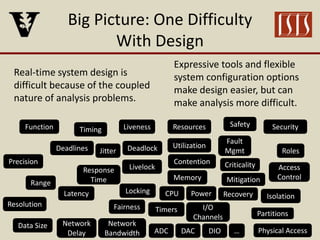
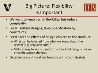
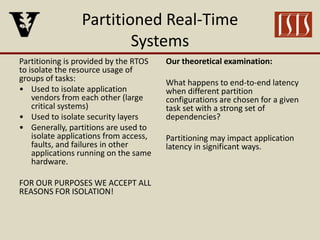
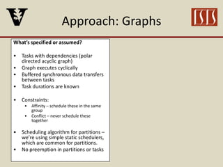
The document discusses partition configuration for real-time systems, highlighting the complexities of design due to task dependencies and resource management. It introduces a framework based on graphs to analyze the impact of different partition configurations on end-to-end latency, emphasizing the importance of isolation and scheduling in real-time systems. Theoretical insights and practical implications for scheduling algorithms and the analysis of task graphs are also presented, along with future work directions.

1. Partition Configuration
for Real-Time Systems
With Dependencies
Joe Porter, Csanad Szabo
Institute for
Software Integrated Systems
Vanderbilt University
Nashville, TN

2. Big Picture: One Difficulty
With Design
Real-time system design is
difficult because of the coupled
nature of analysis problems.
Expressive tools and flexible
system configuration options
make design easier, but can
make analysis more difficult.
Function Timing Liveness Resources Safety Security
Precision
Range
Data Size
Resolution
Deadlines
Latency
Jitter
Response
Time
Network
Delay
Fairness
Deadlock
Livelock
I/O
Channels
ADC DAC DIO
Timers
Utilization
Contention
Network
Bandwidth
CPU
Memory
Power
Fault
Mgmt
Criticality
Partitions
…
Mitigation
Recovery
Roles
Access
Control
Physical Access
Isolation
Locking

3. Big Picture: Flexibility
is Important
• We want to keep design flexibility, but reduce
complexity.
• For RT system designs, favor specification by
constraints
• Feed back the effects of design choices to the modeler
– What can be inferred from what we know about the
system (e.g. requirements)?
– Make it easy to see or predict the effects of design choices
or configuration changes
• Determine configuration bounds within constraints

4. Partitioned Real-Time
Systems
Partitioning is provided by the RTOS
to isolate the resource usage of
groups of tasks:
• Used to isolate application
vendors from each other (large
critical systems)
• Used to isolate security layers
• Generally, partitions are used to
isolate applications from access,
faults, and failures in other
applications running on the same
hardware.
FOR OUR PURPOSES WE ACCEPT ALL
REASONS FOR ISOLATION!
Our theoretical examination:
What happens to end-to-end latency
when different partition
configurations are chosen for a given
task set with a strong set of
dependencies?
Partitioning may impact application
latency in significant ways.

5. Approach: Graphs
What’s specified or assumed?
• Tasks with dependencies (polar
directed acyclic graph)
• Graph executes cyclically
• Buffered synchronous data transfers
between tasks
• Task durations are known
• Constraints:
• Affinity – schedule these in the same
group
• Conflict – never schedule these
together
• Scheduling algorithm for partitions –
we’re using simple static schedulers,
which are common for partitions.
• No preemption in partitions or tasks

6. Approach: Graphs
What’s specified or assumed?
• Tasks with dependencies (polar
directed acyclic graph)
• Graph executes cyclically
• Buffered synchronous data transfers
between tasks
• Task durations are known
• Constraints:
• Affinity – schedule these in the same
group
• Conflict – never schedule these
together
• Scheduling algorithm for partitions –
we’re using simple static schedulers,
which are common for partitions.
• No preemption in partitions or tasks
FRAMEWORK RATIONALE
• Graphs are easy to visualize
• Graphs and constraints are
representationally compatible with our RT
software design tools
• Framework handles all of the relationships
in our problem
• Simple scheduling and non-preemption
because you have to do all of the execution
end-to-end (intend to relax this…)

7. Approach: Graphs
What’s specified or assumed?
• Tasks with dependencies (polar
directed acyclic graph)
• Graph executes cyclically
• Buffered synchronous data transfers
between tasks
• Task durations are known
• Constraints:
• Affinity – schedule these in the same
group
• Conflict – never schedule these
together
• Scheduling algorithm for partitions –
we’re using simple static schedulers,
which are common for partitions.
• No preemption in partitions or tasks
Which quantities are dependent?
• Number of partitions
• Which tasks live in each partition?
(subject to constraints)
• Partition durations and periods
• Application latency (source to sink)
What’s tricky?
• Configuration choices affect the
critical path
• Task graph ordering search problems
are intractible (in general)
• therefore, the layout of tasks within
partitions is also intractable

8. Specifications: Task Graph
and Partitioning Constraints
Task dependency graph (TDG)
G = (V, E)
Task set V = { v0 , … , v6 }
Affinity sets A = { A1 , … , A4 }
No conflicts for now…
Basic Properties
• Consistency – two tasks can have
affinity, or conflict, (or nothing) but
not both
• Partition membership – in the end,
each task will belong to exactly one
partition
• Transitivity – a task in conflict with
one task in an affinity set is also in
conflict with all other members of
the affinity set

9. Specification: Abstractions and
Observations
Affinity Dependency Graph (ADG)
• Current affinity sets are vertices
• Abstracted dependencies
between them:
• at most one edge in each direction
• edge exists if any task dependencies
exist between affinity sets
• NOT ACYCLIC!
Use ADG to make decisions about
grouping tasks into partitions

10. Specification: Abstractions and
Observations
Affinity Dependency Graph (ADG)
• Current affinity sets are vertices
• Abstracted dependencies
between them:
• at most one edge in each direction
• edge exists if any task dependencies
exist between affinity sets
• NOT ACYCLIC!
Merge Operation
• Combine two affinity sets into one
• Remove intervening edges
• Maintain external edges
• Use this to simplify ADGs – why?
Use ADG to make decisions about
grouping tasks into partitions

11. Specification: Abstractions and
Observations
Affinity Dependency Graph (ADG)
• Current affinity sets are vertices
• Abstracted dependencies
between them:
• at most one edge in each direction
• edge exists if any task dependencies
exist between affinity sets
• NOT ACYCLIC!
Back Edge
• In the ADG, a back edge completes one or
more cycles (in the sense of DFS)
• To schedule a back edge, we must revisit
these vertices again in the cycle:
• For harmonic partitions, this means two
or more instances per cycle
• For round-robin partitions, this means
multiple cycles
Partition configuration changes can have
fine-grained effects on end-to-end
latency.
We deliberately avoided those and
considered abstractions that expose
large-impact effects.

12. Specification:
Conflicts and Partitions
Conflict Graphs
Another graph over either the TDG
or the ADG illustrates the defined
conflicts, as shown

13. Theoretical Insights:
Conflicts and Partitions
Conflict Graphs
The number of partitions has to be greater
than or equal to the largest conflict clique.
This is chosen over both graphs, but the
largest ADG conflict clique is never smaller
than the TDG conflict clique, so it’s sufficient
to consider the ADG conflict graph.
The upper bound on the number of
partitions is the number of affinity sets +
the number of unassigned vertices.

14. Theoretical Insights:
Back Edges
Multiple back edges in an ADG do
not necessarily lead to multiple
schedule repetitions:
• repetitions may be scheduled
concurrently
• unless they are nested (shown
above)
• at least one extra repetition will
occur per level of nesting
A few structures always lead to the
formation of back edges in a merge –
in the figure below, affinity sets with
the same labels will be merged.

15. Execution With a Flexible
Partition Scheduler
• In this case, the partition
execution “follows” the task
execution, repeating any
partition as many times as
necessary in the cycle.
• Just perform some useful
ordering of the tasks, and play
them in the right order.
• This gives the tightest result.
At ISIS we now have a partitioned
scheduler for Linux that can be
configured to do it this way, so
this isn’t too far-fetched. It wasn’t
available in time for this paper.

16. Execution With a Harmonic
Partition Scheduler
• This is a standard case for
partition schedulers, and we
solve it with a MILP.
• The tricky part is allowing
tasks to belong to any instance
– this is also encoded in the
MILP (see constraint 7 in the
paper).
• Since each partition instance
has to have the same duration,
the scheduling should be less
tight.
• The MILP objective tries to
squash the extra space as
much as possible.

17. Execution With a Round-Robin
Partition Scheduler
• Round robin partition
scheduling is easy to
implement, and therefore also
common.
• The schedule takes a full cycle
penalty due to the back edge
in the ADG.
• Merging affinity sets A1 and A2
(in the absence of conflict
constraints) would remove the
penalty.
• The conflict relations and the
affinity relations bound the
extremes of partition number,
so we can determine degrees
of freedom in the
configuration problem.
• This gives the longest latency
result.

18. Simulation Environment
TDG Example
• Input TDG is specified in GraphML (with a few slight tweaks)
• Affinity and conflict are included in the graph as attributes on vertices
and edges
• We use the Java JUNG toolkit for graph visualization
• We can generate random problem instances algorithmically
ADG Example

19. Future Work
(and Work In Progress)
Work In Progress
• Validation of predicted
results with F6 OS Linux
partition scheduler
• Automation of the round-
robin analysis
• A real-world application
example
Future Work (or slower
work in progress…)
• Good heuristics for
choosing schedule orders
• Automatic calculation of
nesting depth
• Preemptive task
schedulers
• Multiple local processors
• Distributed processors
with network delays

20. Questions?
Those interested in trying our tools can contact me:
Joe Porter (jporter@isis.vanderbilt.edu)