Downloaded 953 times
![Finite element methods and solid mechanics are the foundation of mechanical simulations. If you haven't taken
these courses, plan to take them after you complete this course of simulation. If you've already taken them and feel
not "solid" enough, review them.
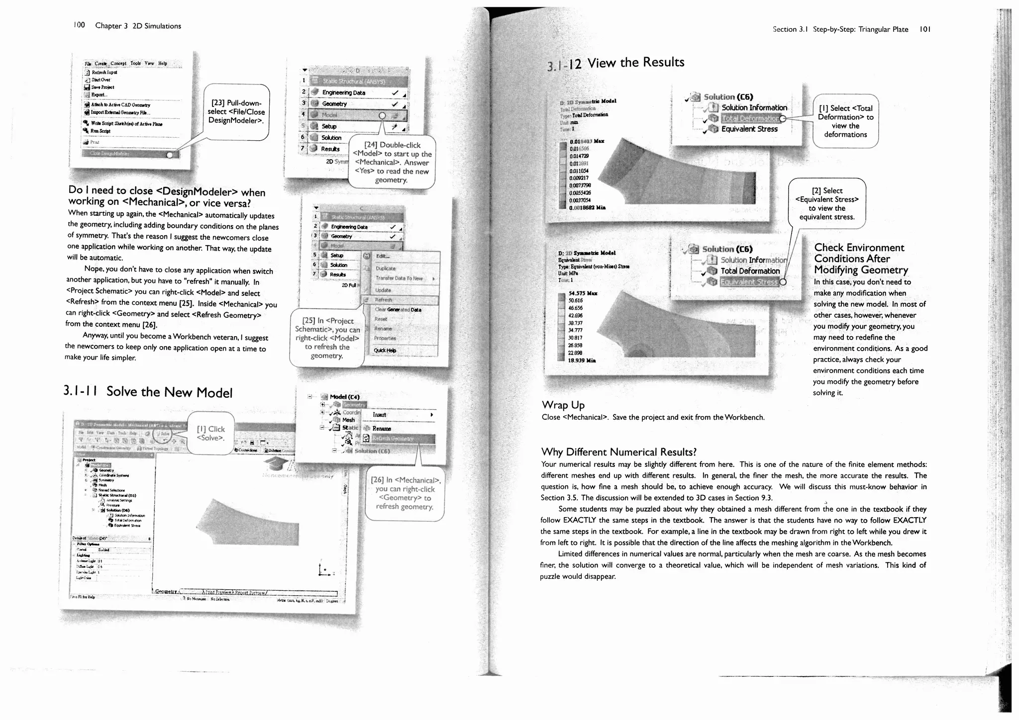
Why Different Numerical Results?
Many students often puzzled because they obtained slightly difference numerical results, but they insist that they
followed exactly the same steps in the textbook. One of the reasons is that different way of creating a geometry may
end up with slightly different mesh, and this in turn ends up with slightly different numerical results. For example, when
you draw a straight line, the order of the end points may affect mesh slightly. Limited differences in numerical values
are normal, particularly when the mesh are coarse. As the mesh becomes finer, the solution will converge to a
theoretical value, which will be independent of mesh variations, and this kind of puzzle should be resolved.
Usage of the Accompanying DVD
The files in the DVD that accompanies with the book is organized according to the chapters and sections of the book.
Each folder of a section stored finished project files for that section. If everything works smoothly, you may not need
the DVD at all. Every project can be built from scratch according to the steps described in the book. We provide this
DVD just in some cases you need it. For examples, when you want to skip the creation of geometry, or when you run
into troubles following the steps and you don't want to redo from the beginning, you may find that these files are
useful. Another situation may happen when you have troubles following the geometry details in the textbook, you may
need to look up the geometry details in the DVD files.
However, It is suggested that, in the beginning of a step-by-step exercise when previously saved project files are
needed, you use the project files stored in the DVD rather than your own files, in order to obtain results that have
exact the same numerical values as shown in the textbook.
Numbering and Self-Reference System
To efficiently present the material, the writing of this textbook is not always done in a traditional format. Chapters and
sections are numbered in a traditional way. Each section is further divided into subsections, for example, the 8th
subsection of the 3rd section of Chapter 4 is denoted as "4.3-8." Each speech bubble in a subsection is assigned a
number. The number is enclosed by a pair of square brackets (e.g., [9]). When needed, we may refer to that speech
bubble such as "4.3-8[9]." When referring to a speech bubble in the same subsection, we drop the subsection
identifier, for the foregoing example, we simply write "[9]." Equations are numbered in a similar way, except that the
equation number is enclosed by a pair of round brackets (parentheses) rather than square brackets. For example,
"1.2-3(2)" refers to the 2nd equation in the Subsection 1.2-3. Numbering notations are summarized as follows:
1.2-3 The number after a hyphen is a subsection number.
[1], [2], ... Square brackets are used to number speech bubbles.
(1), (2), ... These notations are used to number equations
(a), (b), ... These notations are used to number items in the text.
Reference1, 2 Superscripts are used to number references.
<DesignModeler> Angle brackets are used to highlight Workbench keywords.
Workbench Keywords
There are literally thousands of keywords used in the Workbench. For example: DesignModeler, Project Schematic,
etc. To maintain readability and efficiency of the text,Workbench keywords are normally enclosed by a pair of angle
brackets, for examples, <DesignModeler>, <Project Schematic>. Sometimes, however, the angle brackets may be
dropped, whenever it doesn't cause any readability or efficiency problems.
Preface 7](https://image.slidesharecdn.com/huei-huanglee-finiteelementsimulationswithansysworkbench12-2010-151020015452-lva1-app6892/75/Finite-Element-Simulations-with-ANSYS-Workbench-2012-10-2048.jpg)
![10 Chapter 1 Introduction
Section 1.1
Case Study: Pneumatically Actuated
PDMS Fingers1
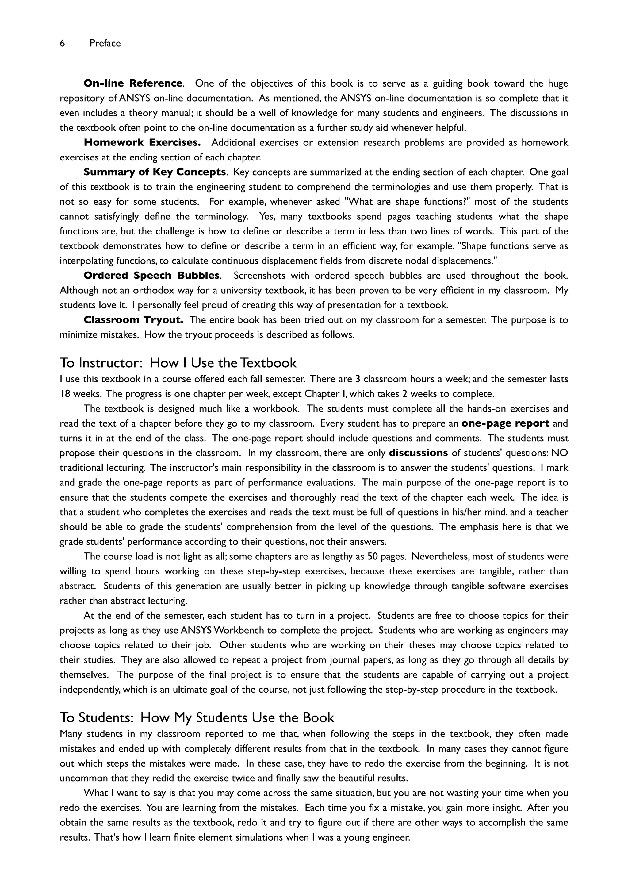
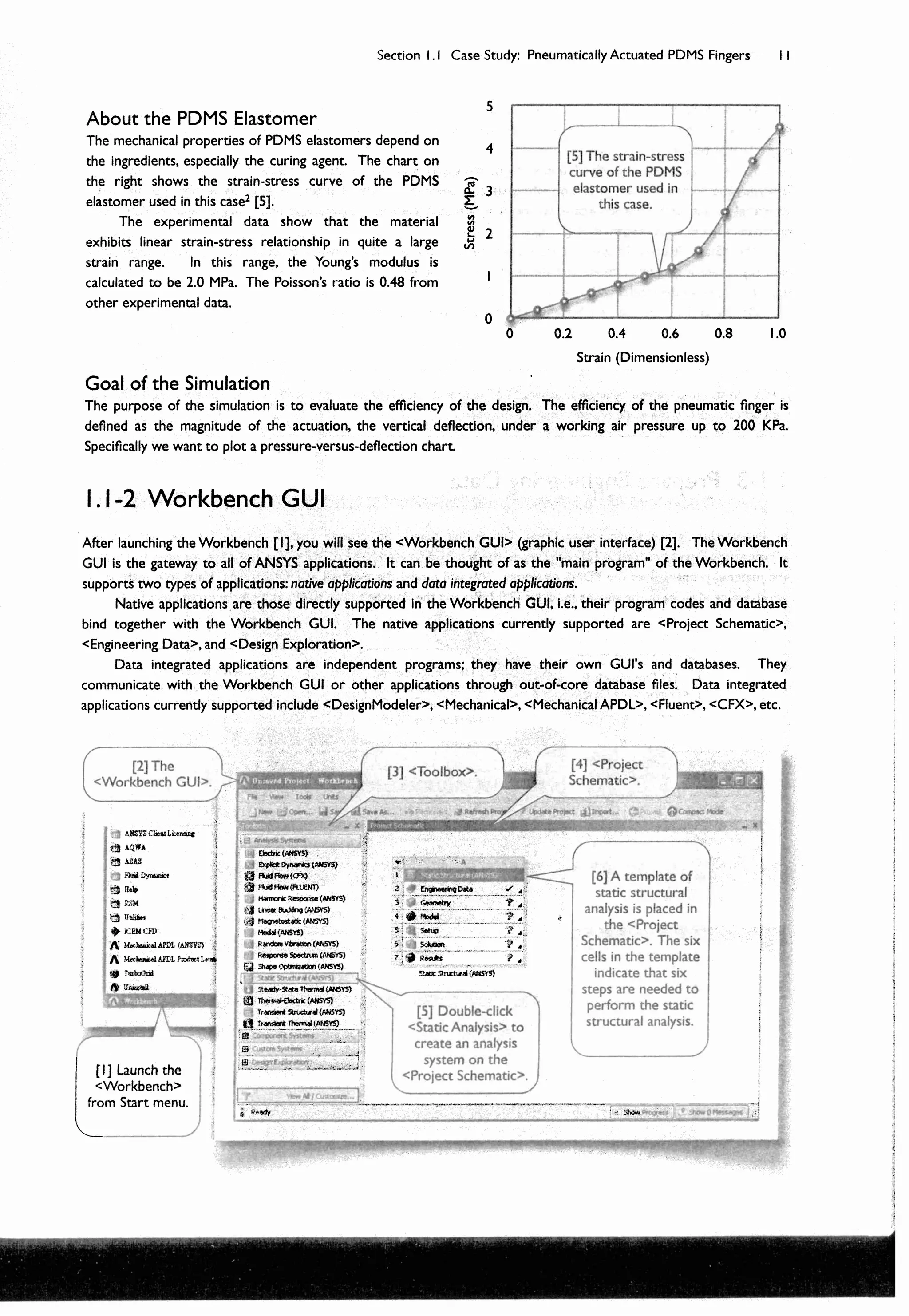
About the Pneumatic Fingers
The pneumatic fingers [1] are designed as part of a surgical parallel robot
system which is remotely controlled by a surgeon through the Internet2.
The robot fingers are made of a PDMS-based (polydimethylsiloxane)
elastomer material. The geometry of a finger is shown in the figure [2]. Note
that 14 air chambers are built in the finger.
The purposes of this section are to (a) overview the functionality of the ANSYS Workbench through a case study, (b)
present an overall structure of the textbook by bringing up topics of the chapters through a case study, and (c) build
motivation for learning the topics in Sections 2, 3, 4 of this chapter: structural mechanics, finite element methods, and
the failure criteria.
Although this case study is presented in a step-by-step fashion, it does not intend to guide the students working
in front of a computer. In fact, only the relevant steps are presented, and some steps are purposely omitted to make
the presentation more instructional. There will be many hands-on exercises in the later chapters. So, be patient.
1.1-1 Problem Description
The chambers are located closer to the upper face than the bottom face so that when the air pressure applies,
the finger bends downward [3]. Note that only half of the model is rendered, so you can see the chambers. The
undeformed model is also shown in the figure [4].
Note: In this book, each speech
bubble has a unique number in a
subsection. The number is
enclosed with a pair of square
brackets. When you read figures,
please follow the order of
numbers; the order is important.
These numbers also serve as
reference numbers when referred.
[1] Five fingers
compose a robot
hand, which is remotely
controlled by a
surgeon.
[2] The finger’s size is
80x5x10.2 (mm). There are 14
air chambers built in the PDMS
finger, each is 3.2x2x8 (mm).
[4] Undeformed
shape.
[3] As the air pressure
applies, the finger bends
downward.](https://image.slidesharecdn.com/huei-huanglee-finiteelementsimulationswithansysworkbench12-2010-151020015452-lva1-app6892/75/Finite-Element-Simulations-with-ANSYS-Workbench-2012-13-2048.jpg)
![Section 2.1 Step-by-Step: W16x50 Beam Section 47
Section 2.1
Step-by-Step: W16x50 Beam
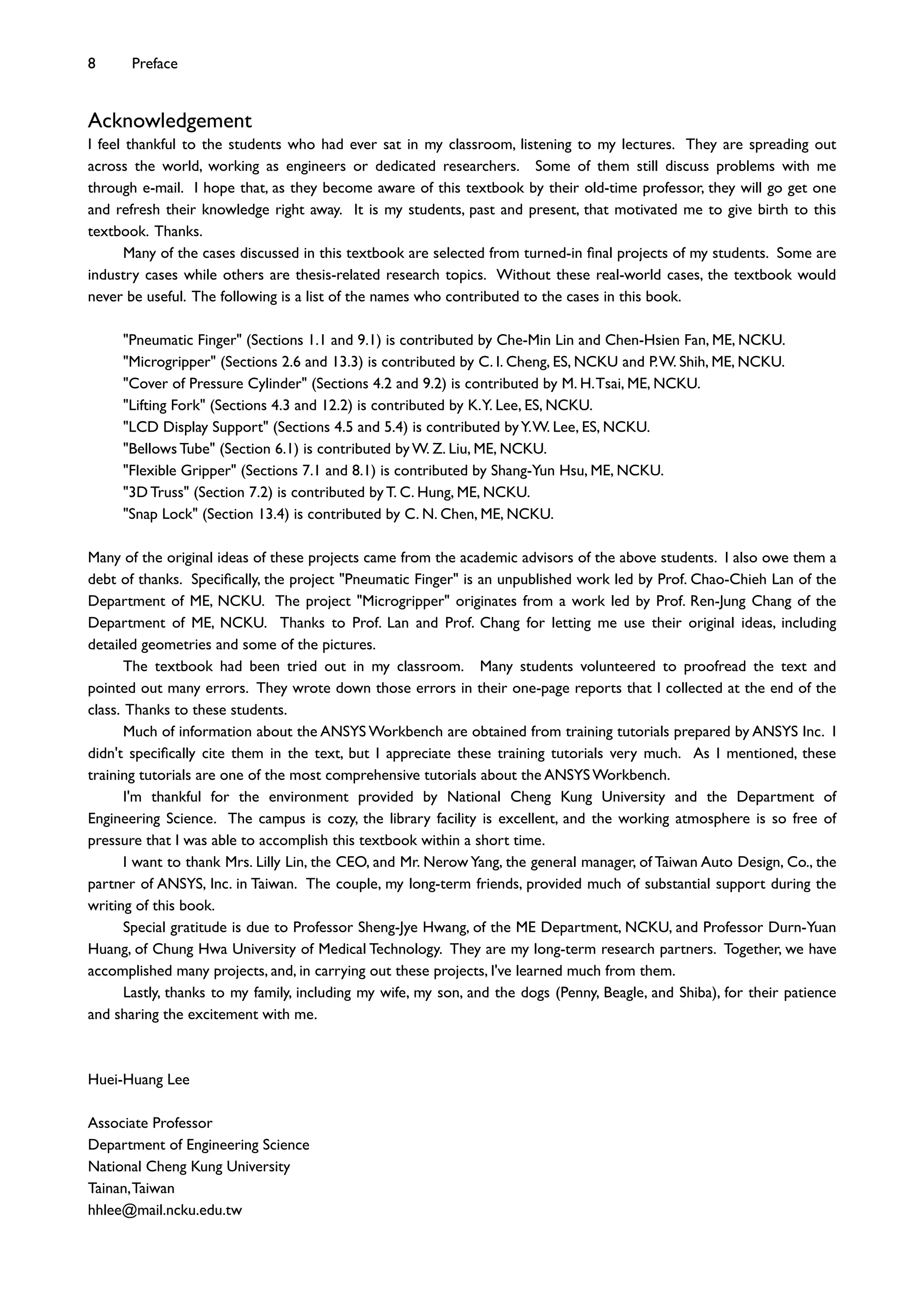
Consider a structural steel beam with a W16x50 cross-section
[1-4] and a length of 10 ft. In this section, we will create a 3D
solid body for the steel beam.
2.1-1 About the W16x50 Beam
W16x50
2.1-2 Start Up <DesignModeler>
16.25"
.628"
.380"
7.07"
R.375"
[1] Wide-;ange
I-shape section.
[2] Nominal
depth 16".
[3] Weight 50
lb/ft.
[4] Detail
dimensions
[2] After a
while, the
<Workbench
GUI> shows up.
[3] Click the
plus sign (+)
to expand the
<Component
Systems>.
Note that the
plus sign
become minus
sign. [4] Double-click
<Geometry> to
place a system in the
<Project
Schematic>.
[6] Double-click
<Geometry> to
start up
DesignModeler.
[5] If anything goes
wrong, click here to
show message.
[1] From Start menu,
click to launch the
Workbench.](https://image.slidesharecdn.com/huei-huanglee-finiteelementsimulationswithansysworkbench12-2010-151020015452-lva1-app6892/75/Finite-Element-Simulations-with-ANSYS-Workbench-2012-34-2048.jpg)
![48 Chapter 2 Sketching
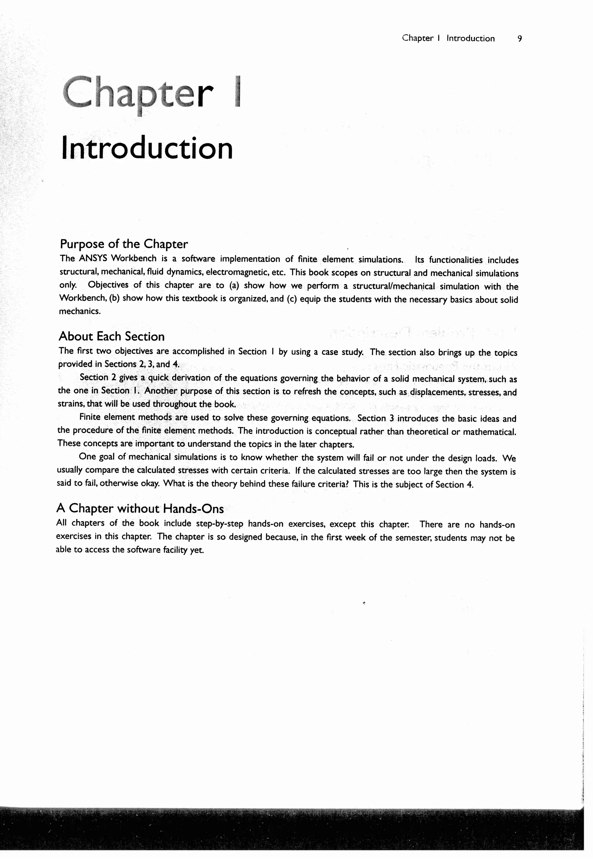
Notes: In a step-by-step exercise, whenever a circle is used with a speech bubble, it is to indicate that mouse or
keynoard ACTIONS must be taken in that step (e.g., [1, 3, 4, 6, 8, 9]). The circle may be small or large, ;lled with
white color or un;lled, depending on whichever gives more information. A speech bubble without a circle (e.g., [2,
7]) or with a rectangle (e.g., [5]) is used for commentary only, no mouse or keyboard actions are needed.
2.1-3 Draw a Rectangle on <XYPlane>
[9] Click <OK>.
Note that, after
clicking <OK>, the
length unit connot be
changed anymore.
[8] Select <Inch> as
the length unit.
[7] After a
while, the
DesignModeler
shows up.
[1] <XYPlane> is
already the
current sketching
plane.
[2] Click
<Sketching> to
enter the
sketching mode.
[4] Click
<Rectangle> tool.
[3] Click <Look
At> to rotate the
coordinate axes, so
that you face the
<XYPlane>.
[5] Draw a
rectangle (using
click-and-drag)
roughly like this.](https://image.slidesharecdn.com/huei-huanglee-finiteelementsimulationswithansysworkbench12-2010-151020015452-lva1-app6892/75/Finite-Element-Simulations-with-ANSYS-Workbench-2012-35-2048.jpg)
![Section 2.1 Step-by-Step: W16x50 Beam Section 49
Impose symmetry constraints...
Specify dimensions...
[6] Click
<Constraint>
toolbox.
[8] Click
<Symmetry>
tool.
[9] Click the vertical
axis and then two
vertical lines on both
sides to make them
symmetric about the
vertical axis.
[10] Right-click
anywhere on the graphic
area to open the context
menu, and choose
<Select new symmetry
axis>.
[11] Click the
horizontal axis and
then two horizontal
lines on both sides
to make them
symmetric about
the horizontal axis.
[7] If you don't
see <Symmetry>
tool, click here to
scroll down to
reveal the tool.
[12] Click
<Dimensions>
toolbox.
[13] Leave
<General> as
the default tool.
[17] In the
<DetailsView>,
type 7.07 (in) for
H1 and 16.25 (in)
forV2.
[14] Click this line,
move the mouse
upward, and click again
to create H1.
[15] Click this line,
move the mouse
rightward, and click
again to createV2.
[17] Click
<Zoom to Fit>.
[16] The segments turn to
blue color. Colors are used
to indicate the constraint
status. The blue color means
that the geometric entities
are well constrained.](https://image.slidesharecdn.com/huei-huanglee-finiteelementsimulationswithansysworkbench12-2010-151020015452-lva1-app6892/75/Finite-Element-Simulations-with-ANSYS-Workbench-2012-36-2048.jpg)
![50 Chapter 2 Sketching
2.1-4 Clean up the Graphic Area
The ruler occupies space and is sometimes annoying; let's turn it off...
Let's display dimension values (in stead of names) on the graphic area...
[2] The ruler
disappears. It creates
more space for the
graphic area. For the
rest of the book, we
always turn off the ruler
to make more space in
the graphic area.
[1] Pull-down-select
<View/Ruler> to
turn the ruler off.
[3] If you
don't see
<Display>
tool, click
here to scroll
all the way
down to the
bottom.
[4] Click
<Display> tool.
[5] Click <Name> to
turn it off. The <Value>
automatically turns on.
[6] The dimension
names are replaced
by the values. For
the rest of the book,
we always display
values instead of
names, so that the
sketching will be
more ef8cient.](https://image.slidesharecdn.com/huei-huanglee-finiteelementsimulationswithansysworkbench12-2010-151020015452-lva1-app6892/75/Finite-Element-Simulations-with-ANSYS-Workbench-2012-37-2048.jpg)
![Section 2.1 Step-by-Step: W16x50 Beam Section 51
2.1-5 Draw a Polyline
Draw a polyline; the dimensions are not important for now...
Copy the newly created polyline to the right side, ;ip horizontally...
2.1-6 Copy the Polyline
[1] Select
<Draw>
toolbox.
[2] Select
<Polyline>
tool.
[3] Click roughly here to
start the polyline. Make sure
a <C> (coincident) appears
before clicking. [4] Click the second point
roughly here. Make sure an
<H> (horizontal) appears
before clicking.
[5] Click the third point
roughly here. Make sure a
<V> (vertical) appears
before clicking.
[6] Click the last point
roughly here. Make sure an
<H> and a <C> appear
before clicking.
[7] Right-click anywhere
on the graphic area to
open the context menu,
and select <Open End> to
end the <Polyline> tool.
[4] Right-click anywhere
on the graphic area to open
the context menu, and select
<End/Use Plane Origin as
Handle>.
[1] Select
<Modify>
toolbox.
[2] Select
<Copy>
tool.
[3] Control-
click (see [11,
12]) the three
newly created
segments one
by one.](https://image.slidesharecdn.com/huei-huanglee-finiteelementsimulationswithansysworkbench12-2010-151020015452-lva1-app6892/75/Finite-Element-Simulations-with-ANSYS-Workbench-2012-38-2048.jpg)
![52 Chapter 2 Sketching
Context menu is used heavily...
Basic Mouse Operations
At this point, let's look into some basic mouse operations [10-16]. Skill of these operations is one of the keys to be
pro<cient at geometric modeling.
[8] Right-click anywhere to
open the context menu again
and select <End> to end the
<Copy> tool. An alternative
way (and better way) is to
press ESC to end a tool.
[9] The
horizontally
=ipped polyline
has been copied.
[6] Right-click anywhere
to open the context
menu again and select
<Flip Horizontal>.
[5] The tool automatically
changes from <Copy> to
<Paste>.
[7] Right-click
anywhere to open the
context menu again and
select <Paste at Plane
Origin>.
[10] Click: single
selection
[11] Control-click:
add/remove selection
[12] Click-sweep:
continuous selection.
[13] Right-click: open
context menu.
[14] Right-click-drag:
box zoom.
[15] Scroll-wheel:
zoom in/out.
[16] Middle-click-drag:
rotation.](https://image.slidesharecdn.com/huei-huanglee-finiteelementsimulationswithansysworkbench12-2010-151020015452-lva1-app6892/75/Finite-Element-Simulations-with-ANSYS-Workbench-2012-39-2048.jpg)
![Section 2.1 Step-by-Step: W16x50 Beam Section 53
2.1-7 Trim Away Unwanted Segments
2.1-8 Impose Symmetry Constraints
[3] Click this
segment to
trim it away.
[4] And click
this segment
to trim it away.
[1] Select <Trim>
tool.
[2] Turn on
<Ignore Axis>. If
you don't turn it
on, the axes will
be treated as
trimming tools.
[2] Select
<Symmetry>.
[3] Click this
horizontal axis and then
two horizontal segments
on both sides as shown
to make them
symmetric about the
horizontal axis.
[1] Select
<Constraints>
toolbox.
[4] Right-click
anywhere to open the
context menu and select
<Select new symmetry
axis>
[5] Click this vertical axis and then two
vertical segments on both sides as shown to
make them symmetric about the vertical
axis. They seemed already symmetric before
we impose this constraint, but the symmetry
is "weak" and may be overridden (destroyed)
by other constraints.](https://image.slidesharecdn.com/huei-huanglee-finiteelementsimulationswithansysworkbench12-2010-151020015452-lva1-app6892/75/Finite-Element-Simulations-with-ANSYS-Workbench-2012-40-2048.jpg)
![54 Chapter 2 Sketching
2.1-9 Specify Dimensions
[2] Leave
<General> as
default tool.
[1] Select
<Dimensions>
toolbox.
[4] Select
<Horizontal>.
[3] Click this
segment and move
leftward to create a
vertical dimension.
Note that the entity is
blue-colored.
[5] Click these
two segments
sequentially and
move upward to
create a
horizontal
dimension.
[6] Type 0.38 for H4
and 0.628 forV3.](https://image.slidesharecdn.com/huei-huanglee-finiteelementsimulationswithansysworkbench12-2010-151020015452-lva1-app6892/75/Finite-Element-Simulations-with-ANSYS-Workbench-2012-41-2048.jpg)
![Section 2.1 Step-by-Step: W16x50 Beam Section 55
2.1-10 Add Fillets
2.1-11 Move Dimensions
[1] Select
<Modify>
toolbox.
[2] Select
<Fillet>
tool. [3] Type 0.375
for the :llet
radius.
[4] Click two
adjacent segments
sequentially to
create a :llet.
Repeat this step
for other three
corners.
[2] Select
<Move>.
[3] Click a
dimension value
and move to a
suitable position
as you like.
Repeat this step
for other
dimensions.
[1] Select
<Dimensions>
toolbox.
[5] The greenish-blue color
of the :llets indicates that
these :llets are under-
constrained. The radius
speci:ed in [3] is a "weak"
dimension (may be destroyed
by other constraints). You
could impose a <Radius>
(which is in <Dimension>
toolbox) to turn the :llets to
blue. We, however, decide to
ignore the color. We want to
show that an under-
constrained sketch can still
be used. In general,
however, it is a good practice
to well-constrain all entities
in a sketch.](https://image.slidesharecdn.com/huei-huanglee-finiteelementsimulationswithansysworkbench12-2010-151020015452-lva1-app6892/75/Finite-Element-Simulations-with-ANSYS-Workbench-2012-42-2048.jpg)
![56 Chapter 2 Sketching
2.1-12 Extrude to Generate 3D Solid
[9] Click
<Zoom to Fit>
whenever
needed.
[10] Click
<Display Plane>
to switch off the
display of
sketching plane.
[11] Click all plus signs
(+) to expand the model
tree and examine the
<Tree Outline>.
[6] Active sketch is
shown here.
[5] The active sketch
(Sketch1) is
automatically chosen
as <Base Object> you
can change to other
sketch if needed.
[2] The model is
now in isometric
view.
[4] Note that the
<Modeling> mode
is automatically
activated.
[7] Type 120
(in) for
<Depth>
[1] Click the little
cyan sphere to
rotate the model in
isometric view for a
better visual effect.
[3] Click
<Extrude>.
[8] Click
<Generate>](https://image.slidesharecdn.com/huei-huanglee-finiteelementsimulationswithansysworkbench12-2010-151020015452-lva1-app6892/75/Finite-Element-Simulations-with-ANSYS-Workbench-2012-43-2048.jpg)
![Section 2.1 Step-by-Step: W16x50 Beam Section 57
2.1-13 Save the Project and Exit Workbench
[1] Click <Save
Project>. Type
"W16x50" as project
name.
[2] Pull-down-select
<File/Close
DesignModeler> to
close DesignModeler.
[3] Alternatively you
can click <Save
Project> in the
<Workbench GUI>.
[4] Pull-down-select
<File/Exit> to
exit Workbench.](https://image.slidesharecdn.com/huei-huanglee-finiteelementsimulationswithansysworkbench12-2010-151020015452-lva1-app6892/75/Finite-Element-Simulations-with-ANSYS-Workbench-2012-44-2048.jpg)
![58 Chapter 2 Sketching
Section 2.2
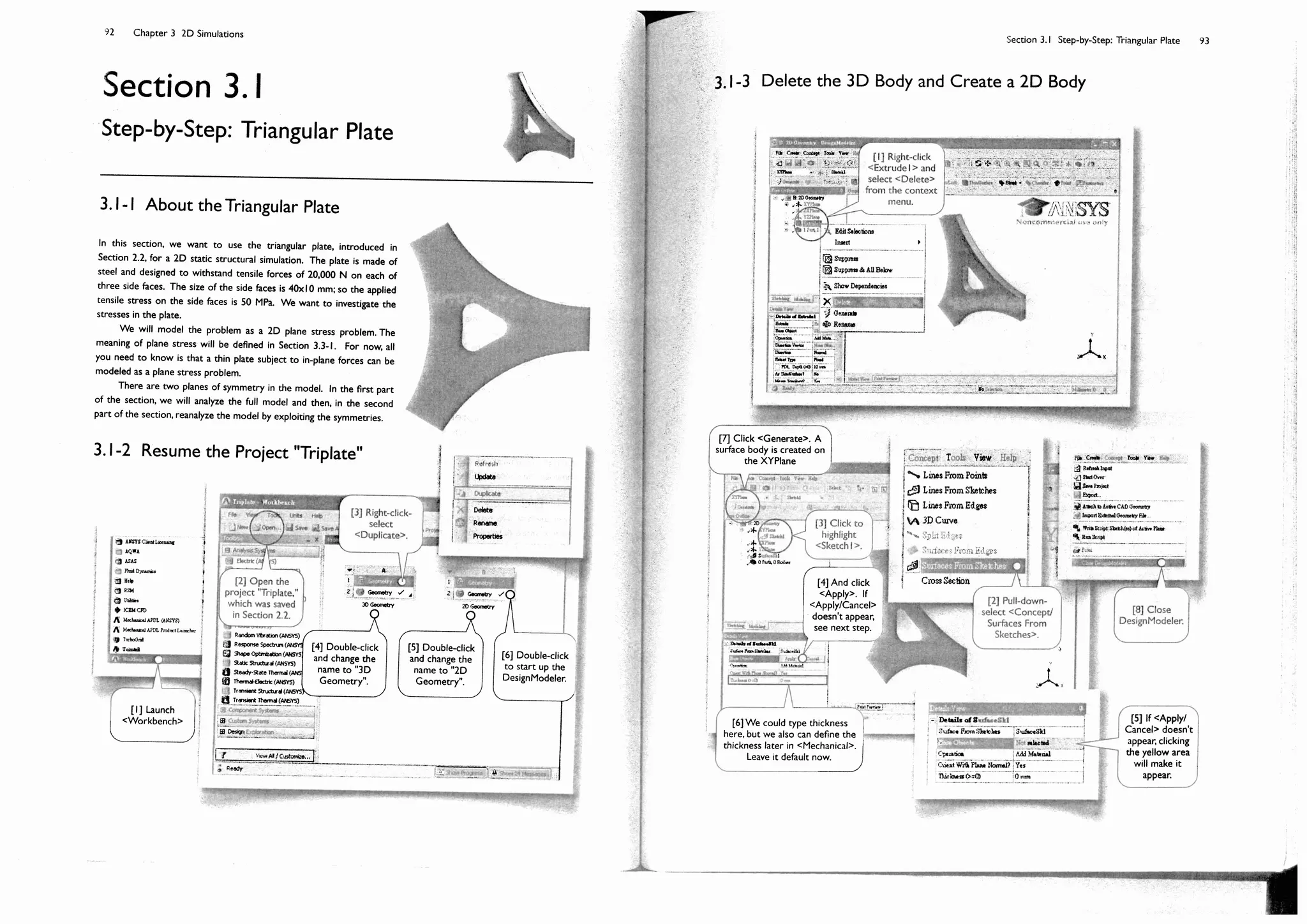
Step-by-Step: Triangular Plate
The triangular plate [1, 2] is made to
withstand a tensile stress of 50 MPa on
each side face [3]. The thickness of the
plate is 10 mm. Other dimensions are
shown in the 7gure.
In this section, we want to sketch
the plate on <XYPlane> and then extrude
a thickness of 10 mm along Z-axis to
generate a 3D solid body.
In Section 3.1, we will use this
sketch again to generate a 2D solid
model, and the 2D model is then used for
a static structural simulation to assess the
stress under the loads.
The 2D solid model will be used
again in Section 8.2 to demonstrate a
design optimization procedure.
2.2-1 About the Triangular Plate
40mm
30 mm
300 mm
2.2-2 Start up <DesignModeler>
[1] From Start
menu, launch the
<Workbench>
[2] Double-click to
create a <Geometry>
system.
[3] Double-click to
start up
<DesignModeler>.
[1] The plate
has three
planes of
symmetry.
[2] Radii of
the 7llets
are 10 mm.
[3] Forces are
applied on
each side face.](https://image.slidesharecdn.com/huei-huanglee-finiteelementsimulationswithansysworkbench12-2010-151020015452-lva1-app6892/75/Finite-Element-Simulations-with-ANSYS-Workbench-2012-45-2048.jpg)
![Section 2.2 Step-by-Step: Triangular Plate 59
2.2-3 Draw a Triangle on <XYPlane>
[6] Select
<Sketching>
mode.
[7] Click <Look
At> to look at
<XYPlane>.
[5] Pull-down-select
<View/Ruler> to turn
the ruler off. For the
rest of the book, we
always turn off the
ruler to make more
space in the graphic
area.
[4] Select
<Millimeter> as
length unit.
[2] Click roughly
here to start a
polyline.
[3] Click the second
point roughly here. Make
sure a <V> (vertical)
constraint appears before
clicking.
[4] Click the third point roughly
here. Make sure a <C> (coincident)
constraint appears before clicking.
<Auto Constraints> is an important
feature of DesignModeler and will
be discussed in Section 2.3-5.
[5] Right-click anywhere
to open the context menu
and select <Close End>
to close the polyline and
end the tool.
[1] Select
<Polyline>
from <Draw>
toolbox.](https://image.slidesharecdn.com/huei-huanglee-finiteelementsimulationswithansysworkbench12-2010-151020015452-lva1-app6892/75/Finite-Element-Simulations-with-ANSYS-Workbench-2012-46-2048.jpg)
![60 Chapter 2 Sketching
Before we proceed, let's spend a few minutes looking into some useful tools for 2D graphics controls [1-10]; feel free
to use these tools whenever needed. The tools are numbered according to roughly their frequency of use. Note that
more useful mouse short-cuts for <Pan>, <Zoom>, and <Box Zoom> are available; please see Section 2.3-4.
2.2-4 Make the Triangle Regular
2.2-5 2D Graphics Controls
[1] Select <Equal
Length> from
<Constraints>
toolbox.
[2] Click these two
segments one after the
other to make their
lengths equal.
[3] Click these two
segments one after the
other to make their
lengths equal.
[9] <Undo>. Click this
tool to undo what you've
just done. Multiple undo
is possible. This tool is
available only in the
<Sketching> mode.
[10] <Redo>. Click this
tool to redo what you've
just undone. This tool is
available only in the
<Sketching> mode.
[2] <Zoom to Fit>.
Click this tool to Bt
the entire sketch in
the graphic area.
[4] <Box Zoom>.
Click to turn on/off
this mode. You can
click-and-drag a box
on the graphic area
to enlarge that
portion of graphics.
[5] <Zoom>. Click to turn on/off
this mode. You can click-and-drag
upward or downward on the
graphic area to zoom in or out.
[1] <Look At>. Click
this tool to make
current sketching
plane rotate toward
you.
[6] <Previous
View>. Click this
tool to go to the
previous view.
[7] <Next
View>. Click this
tool to go to the
next view.
[8] These tools work in
both <Sketching> or
<Modeling> mode.
[3] <Pan>. Click to turn on/off
this mode. You can click-and-
drag on the graphic area to
move the sketch.](https://image.slidesharecdn.com/huei-huanglee-finiteelementsimulationswithansysworkbench12-2010-151020015452-lva1-app6892/75/Finite-Element-Simulations-with-ANSYS-Workbench-2012-47-2048.jpg)
![Section 2.2 Step-by-Step: Triangular Plate 61
2.2-7 Draw an Arc
[2] Select
<Horizontal>.
[6] Select
<Move> and then
move the
dimensions as
you like (Section
2.1-11).
[1] Click <Display> in the
<Dimension> toolbox. Click <Name>
to switch it off and turn <Value> on.
For the rest of the book, we always
display values instead of names.
[3] Click the vertex on the
left and the vertical line on the
right sequentially, and then
move the mouse downward to
create this dimension. Before
clicking, make sure the cursor
changes to indicate that the
point or edge has been
"snapped."
[4] Click the vertex on the left
and the vertical axis, and then
move the mouse downward to
create this dimension. Note that
the triangle turns to blue,
indicating they are well de=ned
now.
[5] In the <DetailsView>,
type 300 and 200 for the
dimensions just created.
Click <Zoom to Fit>
(2.2-5[2]).
[2] Click this
vertex as the
arc center.
Make sure a
<P> (point)
constraint
appears before
clicking.
[3] Click the second point
roughly here. Make sure a
<C> (coincident) constraint
appears before clicking.
[4] Click the
third point
here. Make
sure a <C>
(coincident)
constraint
appears before
clicking.
[1] Select
<Arc by
Center> from
<Draw>
toolbox.
2.2-6 Specify Dimensions](https://image.slidesharecdn.com/huei-huanglee-finiteelementsimulationswithansysworkbench12-2010-151020015452-lva1-app6892/75/Finite-Element-Simulations-with-ANSYS-Workbench-2012-48-2048.jpg)
![62 Chapter 2 Sketching
2.2-8 Replicate the Arc
[2] Click the
arc.
[4] Select this vertex as
paste handle. Make sure
a <P> appears before
clicking.
[1] Select
<Replicate> from
<Modify> toolbox.
Type 120 (degrees)
for <r>. <Replicate>
is equivalent to
<Copy>+<Paste>.
[7] Whenever you have
dif<culty making <P> appear,
click <Selection Filter:
Points> in the toolbar. The
<Selection Filter> also can be
set from the context menu,
see [8].
[3] Right-click
anywhere and select
<End/Set Paste
Handle> in the
context menu.
[8] The <Selection
Filter> also can be
set from the context
menu.[5] Right-click-select
<Rotate by r
Degrees> from the
context menu.
[6] Click this vertex to
paste the arc. Make sure a
<P> appears before
clicking. If you have
dif<culty making <P>
appear, see [7, 8].](https://image.slidesharecdn.com/huei-huanglee-finiteelementsimulationswithansysworkbench12-2010-151020015452-lva1-app6892/75/Finite-Element-Simulations-with-ANSYS-Workbench-2012-49-2048.jpg)
![Section 2.2 Step-by-Step: Triangular Plate 63
For instructional purpose, we chose to manually set the paste handle [3] on the vertex [4]. We could have used plane
origin as handle. In fact, that would have been easier since we wouldn't have to struggle to make sure whether a <P>
appears or not. Whenever you have dif;culty to "snap" a particular point, you should take advantage of <Selection
Filter> [7, 8].
2.2-9 Trim Away Unwanted Segments
[10] Click this vertex to
paste the arc. Make sure
a <P> appears before
clicking (see [7, 8]).
[9] Right-click-select
<Rotate by r
Degrees> in the
context menu.
[11] Right-click-select
<End> in the context
menu to end <Replicate>
tool. Alternatively, you
may press ESC to end a
tool.
[3] Click to trim
unwanted segments
as shown, totally 6
segments are
trimmed away.
[1] Select <Trim>
from <Modify>
toolbox.
[2] Turn on
<Ignore Axis>.](https://image.slidesharecdn.com/huei-huanglee-finiteelementsimulationswithansysworkbench12-2010-151020015452-lva1-app6892/75/Finite-Element-Simulations-with-ANSYS-Workbench-2012-50-2048.jpg)
![64 Chapter 2 Sketching
2.2-11 Specify Dimension of Side Faces
After impose dimension in [2],
the arcs turns to blue, indicating
they are well de;ned now.
Note that we didn't specify the
radii of the arcs; after well
de;ned, the radii of the arcs can
be calculated from other
dimensions.
Constraint Status
Note the arcs have a greenish-
blue color, indicating they are
not well de;ned yet (i.e., under-
constrained). Other color
codes are: blue and black
colors for well de;ned entities
(i.e., ;xed in the space); red
color for over-constrained
entities; gray to indicate an
inconsistency.
[1] Select <Equal
Length> from
<Constraints>
toolbox
[5] Click the
horizontal axis as
the line of
symmetry.
[4] Select
<Symmetry>.
[2] Click this segment and
the vertical segment
sequentially to make their
lengths equal.
[3] Click this segment and
the vertical segment
sequentially to make their
lengths equal.
[6] Click the
lower and upper
arcs sequentially to
make them
symmetric.
[1] Select <Dimension>
toolbox and leave
<General> as default.
[2] Click the
vertical segment
and move the
mouse rightward to
create this
dimension.
[3] Type 40 for the
dimension just
created.
2.2-10 Impose Constraints](https://image.slidesharecdn.com/huei-huanglee-finiteelementsimulationswithansysworkbench12-2010-151020015452-lva1-app6892/75/Finite-Element-Simulations-with-ANSYS-Workbench-2012-51-2048.jpg)
![Section 2.2 Step-by-Step: Triangular Plate 65
2.2-12 Create Offset
[1] Select <Offset>
from <Modify>
toolbox.
[2] Sweep-select all the
segments (sweep each segment
while holding your left mouse
button down, see 2.1-6[12]).
After selected, the segments turn
to yellow. Sweep-select is also
called paint-select.
[4] Right-click-select
<End selection/Place
Offset> in the
context menu.
[6] Right-click-select
<End> in the context
menu, or press ESC,
to close <Offset>
tool.
[5] Click roughly
here to place the
offset.
[3] Another way to select
multiple entities is to switch the
<Select Mode> to <Box
Select>, and then draw a box to
select all entities inside the box.](https://image.slidesharecdn.com/huei-huanglee-finiteelementsimulationswithansysworkbench12-2010-151020015452-lva1-app6892/75/Finite-Element-Simulations-with-ANSYS-Workbench-2012-52-2048.jpg)
![66 Chapter 2 Sketching
2.2-13 Create Fillets
[1] Select <Fillet>
in <Modify> toolbox.
Type 10 (mm) for the
<Radius>.
[7] Select
<Horizontal> from
<Dimension>
toolbox.
[8] Click the two left arcs
and move downward to create
this dimension. Note the offset
turns to blue.
[9] Type 30 for
the dimension
just created.
[10] It is possible that these two
point become separate now. If
so, impose a <Coincident>
constraint on them, see [11].
[11] If necessary,
impose a
<Coincident> on
the separate
points.
[2] Click These two segments
sequentially to create a 7llet.
Repeat this step to create the
other two 7llets. Note that
the 7llets are in greenish-blue
color, indicating they are not
well de7ned yet.](https://image.slidesharecdn.com/huei-huanglee-finiteelementsimulationswithansysworkbench12-2010-151020015452-lva1-app6892/75/Finite-Element-Simulations-with-ANSYS-Workbench-2012-53-2048.jpg)
![Section 2.2 Step-by-Step: Triangular Plate 67
2.2-14 Extrude to Create 3D Solid
[4] Select
<Radius> from
<Dimension>
toolbox.
[3] Dimensions
speci6ed in a
toolbox are usually
regarded as "weak"
dimensions,
meaning they may
be changed by
imposing other
constraints or
dimensions.
[5] Click one of the 6llets
and move upward to create
this dimension. This action
turns a "weak" dimension to
a "strong" one. The 6llets
turn blue now.
[2] Click
<Extrude>.
[1] Click the little
cyan sphere to
rotate the model in
isometric view, to
have a better view.
[3] Type 10
(mm) for
<Depth>.
[4] Click
<Generate>.
[5] Click <Display Plane>
to turn off the display of
sketching plane.
[6] Click all plus
signs (+) to
expand and
examine the
<Tree Outline>.](https://image.slidesharecdn.com/huei-huanglee-finiteelementsimulationswithansysworkbench12-2010-151020015452-lva1-app6892/75/Finite-Element-Simulations-with-ANSYS-Workbench-2012-54-2048.jpg)
![68 Chapter 2 Sketching
2.2-15 Save the Project and Exit Workbench
[1] Click <Save
Project>. Type
"Triplate" as project
name.
[2] Pull-down-select
<File/Close
DesignModeler> to
close DesignModeler.
[3] Alternatively you
can click <Save
Project> in the
<Workbench GUI>.
[4] Pull-down-select
<File/Exit> to
exit Workbench.](https://image.slidesharecdn.com/huei-huanglee-finiteelementsimulationswithansysworkbench12-2010-151020015452-lva1-app6892/75/Finite-Element-Simulations-with-ANSYS-Workbench-2012-55-2048.jpg)
![Section 2.3 More Details 69
Section 2.3
More Details
2.3-1 DesignModeler GUI
The DesignModeler GUI is composed of several areas [1-7]. On the top are pull-down menus and toolbars [1]; on the
bottom is a status bar [7]. In-between are several "window panes". A separator [8] between two window panes can
be dragged to resize the window panes. You even can move or dock a pane by dragging its title bar. Whenever you
mess up the workspace, simply pull-down-select <View/Windows/Reset Layout> to reset the default layout.
The <Tree Outline> [3] shares the same area with the <Sketching Toolboxes> [4]; you switch between these two
"modes" by clicking the "mode tab" [2]. The <Details View> [6] shows the detail information of the geometry you
currently work with. The graphics area [5] displays the model when in <Model View> mode; you can click a tab to
switch to <Print Preview>. We will cover more details of DesignModeler GUI in Chapter 4.
Model Tree
The <Tree Outline> contains an outline of the model tree, the tree representation of the geometric model. Each leaf
and branch of the tree is called an object. A branch is an object containing one or more objects under itself. A model
tree consists of planes, features, and a part branch. The parts are the only objects that are exported to <Mechanical>.
Right-clicking an object and select a tool from the context menu, you can operate on the object, such as delete,
rename, duplicate, etc.
[1] Pull-down menus
and toolbars.
[3] <Tree
Outline>, in
<Modeling>
mode.
[6] <Details
View>.
[5] Graphics area.
[7] Status bar
[4] <Sketching
Toolboxes> in
<Sketching> mode.
[2] Mode tabs.
[8] A
separator
allow you to
resize the
window
panes.](https://image.slidesharecdn.com/huei-huanglee-finiteelementsimulationswithansysworkbench12-2010-151020015452-lva1-app6892/75/Finite-Element-Simulations-with-ANSYS-Workbench-2012-56-2048.jpg)
![70 Chapter 2 Sketching
A sketch consists of points and edges; edges may be straight lines or curves. Along with these geometric entities, there
are dimensions and constraints imposed on these entities. As mentioned (Section 2.3-2), multiple sketches may be
created on a plane. To create a new sketch on a plane on which there is yet no sketches, you simply switch to
<Sketching> mode and draw any geometric entities on it. Later, if you want to add a new sketch on that plane, you
need to click <New Sketch> [3]. Only one plane and one sketch is active at a time [1, 2]: newly created sketches are
added to the active plane, and newly created geometric entities are added to the active sketch. In this chapter, we only
work with a single sketch which is on the <XYPlane>. More on creating sketches will be discussed in Chapter 4.
When a new sketch is created, it becomes the active sketch.
Sketches are created on sketching planes, or simply planes. Each sketch must be associated with a plane; each plane may
have multiple sketches on it. In the beginning of a DesignModeler session, three planes are created automatically:
<XYPlane>, <YZPlane>, and <ZXPlane>. Currently active plane is shown on the toolbar [1]. You can create new
planes as needed [2]. There are many ways of creating a new plane [3]. In this chapter, since we assume sketches are
created on the <XYPlane>, we will not discuss how to create sketching planes further, which will be discussed in
Chapter 4. Usage of planes is not limited for storing sketches. Section 4.3-8 demonstrates another usage of planes.
2.3-2 Sketching Planes
2.3-3 Sketches
The order of the objects is often relevant. DesignModeler renders the geometry according to the order. New
objects are normally added one-by-one before the parts branch. If you want to insert a new object BEFORE an
existing object, right-click the existing object and select <Insert/...> from the context menu. After insertion,
DesignModeler will re-render the geometry again.
[1] Currently
active plane is
<XYPlane>
[2]You can click
<New Plane> to
create a new plane.
[3]You can choose many
ways of creating a new
plane.
[3]You can click <New
Sketch> to create a sketch on
the active sketching plane.
[1] Currently
active sketching
plane.
[2] Currently
active sketch.
[4] Active sketching
plane can be changed
using the pull-down list,
or by selection from the
<Tree Outline>.
[5] Active sketch can be
changed using the pull-
down list, or by selection
from the <Tree
Outline>.](https://image.slidesharecdn.com/huei-huanglee-finiteelementsimulationswithansysworkbench12-2010-151020015452-lva1-app6892/75/Finite-Element-Simulations-with-ANSYS-Workbench-2012-57-2048.jpg)
![Section 2.3 More Details 71
2.3-4 Sketching Toolboxes
When you switch to <Sketching> mode by clicking the mode tab (2.3-1[2]), you will see a <Sketching Toolboxes>
(2.3-1[4]). The <Sketching Toolboxes> consists of ;ve toolboxes: <Draw>, <Modify>, <Dimensions>, <Constraints>,
and <Settings> [1-5]. Most of the tools in the toolboxes are self-explained. The most ef;cient way to learn the tools
is to try them out. During the tryout, whenever you want to clean up the graphics area, pull-down-select <File/Start
Over>, or select all entities and then delete them. Some tools need further explanation, as described in the rest of
this section.
Before we jump to discuss each of the toolboxes, some tips relevant to sketching are worth emphasizing ;rst.
Pan, Zoom, and Box Zoom
Besides the <Pan> tool (2.2-5[3]), the graphics can be panned by dragging your mouse while holding down both
control key and the middle mouse button. Besides the <Zoom> tool (2.2-5[5]) the graphics can be zoomed in/out by
simply rolling forward/backward your mouse wheel. The <Box Zoom> (2.2-5[4]) can be done by right-clicking and
then dragging a rectangle in the graphics area. When you get use to these basic mouse actions, you probably don't
need <Pan>, <Zoom>, and <Box Zoom> tools in the toolbar any more.
Context Menu
While most of operations can be done by issuing commands using pull-down menus or toolbars, many operations
either require or are more ef;cient using the context menu. The context menu can be popped-up by right-clicking the
graphics area or objects in the model tree. Try to explore whatever available in the context menu.
Status Bar
The status bar (2.3-1[7]) contains instructions on completing each operations. Look at the instruction whenever you
wonder about what actions to do next. The coordinates of your mouse pointer are also shown in the status bar; they
are sometimes useful.
[1] <Draw>
toolbox.
[2] <Modify>
toolbox. [3] <Dimensions>
toolbox.
[4] <Constraints>
toolbox.
[5] <Settings>
toolbox.](https://image.slidesharecdn.com/huei-huanglee-finiteelementsimulationswithansysworkbench12-2010-151020015452-lva1-app6892/75/Finite-Element-Simulations-with-ANSYS-Workbench-2012-58-2048.jpg)
![72 Chapter 2 Sketching
2.3-5 Auto Constraints1, 2
By default, DesignModeler is in <Auto Constraints> mode, both
globally and locally. While drawing, DesignModeler attempts to
detect the user's intentions and try to automatically impose
constraints on the points or edges. The following cursor symbols
indicate the kind of constraints that will be applied:
C - The point is coincident with a line.
P - The point is coincident with another point.
H - The line is horizontal.
V - The line is vertical.
// - The line is parallel to another line.
T - The point is a tangent point.
- The point is a perpendicular foot.
R - The circle's radius is equal to another circle's.
Both <Global> and <Cursor> modes are based on all entities of the
active plane, not just the active sketch. The difference is that
<Cursor> mode only examines the entities nearby the cursor, while
<Global> mode examines all the entities in the active plane.
Note that while <Auto Constraints> can be useful, they
sometimes can lead to problems and add noticeable time on
complicated sketches. Turn off them if desired [1].
2.3-6 <Draw> Tools3
Line by 2 Tangents
Select two curves, a line tangent to these two curves will be created.
The curves can be circle, arc, ellipse, or spline.
Oval
The >rst two clicks de>ne the two centers, and the third click de>nes
the radius.
Circle by 3 Tangents
Select three edges, then a circle tangent to these three edges will be
created. Remember that an edge can be a line or a curve.
Arc by Tangent
Click a point on an edge, an arc starting from that point and tangent
to that edge will be created; click a second point to de>ne the other
end point of the arc.
Spline
A spline is either rigid or ?exible. The difference is that a ?exible
spline can be edited or changed by imposing constraints, while a rigid
spline cannot. After de>ning the last point, you must right-click to
open the context menu, and select an option [2]: either open end or
closed end; either with >t points or without >t points.
[1] By default,
DesignModeler is in
<Auto Constraints>
mode, both globally and
locally. You can turn
them off whenever
cause troubles.
[1] <Draw>
toolbox.](https://image.slidesharecdn.com/huei-huanglee-finiteelementsimulationswithansysworkbench12-2010-151020015452-lva1-app6892/75/Finite-Element-Simulations-with-ANSYS-Workbench-2012-59-2048.jpg)
![Section 2.3 More Details 73
Construction Point at Intersection
Select two edges, a construction point will be created at the
intersection.
Delete Entities
There are no tools in the <Sketching Toolboxes> to delete entities. To
delete entities, select them and right-click-select <Delete>. Multiple
selection methods (e.g., control-selection and sweep-selection, see
Section 2.1-6 and 2.2-12[2]), can be used to select entities.
Abort a Tool
To cancel a tool in any of toolbox, simply press <ESC>.
2.3-7 <Modify> Tools4
Corner
Click two entities, which can be lines or curves, the entities will be
trimmed or extended up to the intersection point and form a sharp
corner. The clicking points decide which sides to be trimmed.
Split
This tool split an edge into several segments depending on the options
[2]. <Split Edge at Selection>: you click an edge, the edge will be split
at the clicking point. <Split Edges at Point>: you click a point, all the
edges passing through that point will be split at that point. <Split Edge
at All Points>: you select an edge, the edge will be split at all points on
the edge. <Split Edge into n Equal Segments>:You specify the value n,
and select an edge, the edge will be split equally into n segments.
Drag
Drag a point or an edge to a new position. All the constraints and
dimensions are preserved.
Cut
It is the same as <Copy>, except the originals are deleted.
Move
It is equivalent to a <Cut> followed by a <Paste>.
Replicate
It is equivalent to a <Copy> followed a <Paste>.
Duplicate
It is equivalent to <Replicate>, except the entities are pasted on the
same place as the originals and become part of the current sketch. It
is often used to duplicate plane boundaries.
Spline Edit
It is used to modify 7exible splines. You can insert, delete, drag the 6t
points, etc. For details, see the reference4.
[2] Right-click and
select one of the
options to
complete the
<Spline> tool.
[1] <Modify>
toolbox.
[2] Context
menu for
<Split> tool.
[3] Context
menu for <Spline
Edit>.](https://image.slidesharecdn.com/huei-huanglee-finiteelementsimulationswithansysworkbench12-2010-151020015452-lva1-app6892/75/Finite-Element-Simulations-with-ANSYS-Workbench-2012-60-2048.jpg)
![74 Chapter 2 Sketching
2.3-8 <Dimensions> Tools5
Semi-Automatic
This tool will display a series of dimensions automatically to help you
fully dimension the sketch.
Edit
Click a dimension name or value, it allows you to change its name or
value.
2.3-9 <Constraints> Tools6
Fixed
It applies on any entity to make it fully constrained.
Horizontal
It applies on a line to make it horizontal.
Vertical
It applies on a line to make it vertical.
Perpendicular
It applies on two edges to make them perpendicular to each other.
Tangent
It applies on two edges, one of which must be a curve, to make them
tangent to each other.
Coincident
Select two points to make them coincident. Select a point and an
edge, the edge or its extension will pass through the point. There are
other possibilities, depending on how you select the entities.
Midpoint
Select a line and then a point, the midpoint of the line will coincide
with the point.
Symmetry
Select a line or an axis, as the line of symmetry, and either select 2
points or 2 lines. If select 2 points, the points will be symmetric about
the line of symmetry. If select 2 lines, the lines will form the same
angle with the line of symmetry.
Parallel
It applies on two lines to make them parallel to each other.
[1] <Dimension>
toolbox.
[1] <Constraints>
toolbox.](https://image.slidesharecdn.com/huei-huanglee-finiteelementsimulationswithansysworkbench12-2010-151020015452-lva1-app6892/75/Finite-Element-Simulations-with-ANSYS-Workbench-2012-61-2048.jpg)
![Section 2.3 More Details 75
Concentric
It applies on two curves, which may be circle, arc, or ellipse, to make
their centers coincident.
Equal Radius
It applies on two curves, which may be circle or arc, to make their
radii equal.
Equal Length
It applies on two lines to make their lengths equal.
Equal Distance
It applies on two distances to make them equal. A distance can be
de6ned by selecting two points, two parallel lines, or one point and
one line.
2.3-10 <Settings> Tools7
[2]You can turn on
the grid display.
References
1. ANSYS Help System>DesignModeler>2D Sketching>Auto Constraints
2. ANSYS Help System>DesignModeler>2D Sketching>Constraints Toolbox>Auto Constraints
3. ANSYS Help System>DesignModeler>2D Sketching>Draw Toolbox
4. ANSYS Help System>DesignModeler>2D Sketching>Modify Toolbox
5. ANSYS Help System>DesignModeler>2D Sketching>Dimensions Toolbox
6. ANSYS Help System>DesignModeler>2D Sketching>Constraints Toolbox
7. ANSYS Help System>DesignModeler>2D Sketching>Settings Toolbox
[1] <Settings>
toolbox.
[3]You can turn on
the snap capability.
[4] If you turn on
the grid display, you
can specify the grid
spacing.
[5] If you turn on
the snap capability,
you can specify the
snap spacing.](https://image.slidesharecdn.com/huei-huanglee-finiteelementsimulationswithansysworkbench12-2010-151020015452-lva1-app6892/75/Finite-Element-Simulations-with-ANSYS-Workbench-2012-62-2048.jpg)
![76 Chapter 2 Sketching
Section 2.4
Exercise: M20x2.5 Threaded Bolt
Consider a pair of threaded bolt and nut. The bolt has external threads while the nut has internal threads. This
exercise is to created a sketch and revolve the sketch 360 to generate a solid body for a portion of the bolt [1]
threaded with M20x2.5 [2-6]. In Section 3.2, we will use this sketch again to generate a 2D solid model. The 2D
model is then used for a static structural simulation.
2.4-1 About the M20x2.5 Threaded Bolt
M20x2.5
H = ( 3 2)p = 2.165 mm
d1
= d (5 8)H 2 =17.294 mm
External
threads
(bolt)
Internal
threads
(nut)
H
H
4
H
8
32
11p=27.5
p
p
d1
d
Minor diameter of internal thread d1
Nominal diameter d
60o
[2] Metric
system.
[3] Nominal
diameter
d = 20 mm.
[4] Pitch
p = 2.5 mm.
[1] The threaded bolt
created in this
exercise.
[5] Thread
standards.
[6] Calculation
of detail sizes.](https://image.slidesharecdn.com/huei-huanglee-finiteelementsimulationswithansysworkbench12-2010-151020015452-lva1-app6892/75/Finite-Element-Simulations-with-ANSYS-Workbench-2012-63-2048.jpg)
![Section 2.4 Exercise: M20x2.5 Threads 77
2.4-2 Draw a Horizontal Line
2.4-3 Draw a Polyline
Draw a polyline (totally 3 segments) and specify dimensions (30o
, 60o
, 60o
, 0.541, and 2.165) as shown below. Note
that, to avoid confusion, we explicitly specify all the dimensions. You may apply constraints instead. For example, using
<Parallel> constraint in stead of specifying an angle dimension [1].
Launch <Workbench>. Create a <Geometry>
System. Save the project as "Threads." Start up
<DesignModeler>. Select <Millimeter> as length
unit.
Draw a horizontal line on the <XYPlane>.
Specify the dimensions as shown [1].
[1] Draw a
horizontal line
with dimensions
as shown.
[1]You may impose a
<Parallel> constraint
on this line instead of
specifying the angle.](https://image.slidesharecdn.com/huei-huanglee-finiteelementsimulationswithansysworkbench12-2010-151020015452-lva1-app6892/75/Finite-Element-Simulations-with-ANSYS-Workbench-2012-64-2048.jpg)
![78 Chapter 2 Sketching
2.4-4 Draw Fillets
Draw two vertical lines and specify their
positions (0.271 and 0.541). Draw an arc
using <Arc by 3 Points>. If the arc is not
in blue color, impose a <Tangent>
constraint on the arc and one of its
tangent line [1].
2.4-5 Trim Unwanted Segments
2.4-6 Replicate 10 Times
Select all segments except the horizontal one (totally 4
segments), and replicate 10 times. You may need to manually
set the paste handle [1]. You may also need to use the tool
<Selection Filter: Points> [2].
[1] Tangent
point.
[1] Set Paste
Handle at this
point.
[2] <Selection
Filter: Points>.
[1] The sketch
after trimming.](https://image.slidesharecdn.com/huei-huanglee-finiteelementsimulationswithansysworkbench12-2010-151020015452-lva1-app6892/75/Finite-Element-Simulations-with-ANSYS-Workbench-2012-65-2048.jpg)
![Section 2.4 Exercise: M20x2.5 Threads 79
2.4-7 Complete the Sketch
Follow the steps [1-5] to complete the
sketch. Note that, in step [4], you don't need
to worry about the length. After step [5],
you can trim the vertical segment created in
step [4].
2.4-8 Revolve to Create 3D Solid
References
1. Zahavi, E., The Finite Element Method in Machine Design, Prentice-Hall, 1992; Chapter 7. Threaded Fasteners.
2. Deutschman,A. D., Michels,W. J., and Wilson, C. E., Machine Design:Theory and Practice, Macmillan Publishing Co.,
Inc., 1975; Section 16-6. Standard Screw Threads.
Revolve the sketch to generate a solid of
revolution. Select theY-axis as the axis of
revolution.
Save the project and exit from the
Workbench. We will resume this project
again in Section 3.2.
[1] Create this
segment by
using
<Replicate>.
[3] Specify this
dimension.
[2] Draw this
segment, which
passes through
the origin.
[4] Draw this
vertical
segment. You
can trim it
after next
step.
[5] Draw this
horizontal
segment.](https://image.slidesharecdn.com/huei-huanglee-finiteelementsimulationswithansysworkbench12-2010-151020015452-lva1-app6892/75/Finite-Element-Simulations-with-ANSYS-Workbench-2012-66-2048.jpg)
![80 Chapter 2 Sketching
The 8gure below shows a pair of identical spur gears in mesh [1-12]. Spur gears have their teeth cut parallel to the
axis of the shaft on which the gears are mounted. Spur gears are used to transmit power between parallel shafts. In
order that two meshing gears maintain a constant angular velocity ratio, they must satisfy the fundamental law of
gearing: the shape of the teeth must be such that the common normal at the point of contact between two teeth must
always pass through a 8xed point on the line of centers1 [5]. This 8xed point is called the pitch point [6].
The angle between the line of action and the common tangent [7] is known as the pressure angle [8]. The
parameters de8ning a spur gear are its pitch radius (rp = 2.5 in) [3], pressure angle ( = 20o
) [8], and number of teeth
(N = 20). In addition, the teeth are cut with a radius of addendum ra = 2.75 in [9] and a radius of dedendum rd = 2.2 in
[10]. The shaft has a radius of 1.25 in [11]. The 8llet has a radius of 0.1 in [12]. The thickness of the gear is 1.0 in.
2.5-1 About the Spur Gears
Section 2.5
Exercise: Spur Gears
Geometric details of spur gears are important for a mechanical engineer. However, if you are not concerned about
these geometric details for now, you may skip the 8rst two subsections and jump directly to Subsection 2.5-3.
[7] Common
tangent of the
pitch circles.
[6] Contact
point (pitch
point).
[8] Line of action (common
normal of contacting gears).
The pressure angle is 20o
.
[3] Pitch circle
rp = 2.5 in.
[9] Addendum
ra = 2.75 in.
[10]
Dedendum
rd = 2.2 in.
[1] The driving
gear rotates
clockwise.
[2] The driven
gear rotates
counter-
clockwise.
[4] Pitch
circle of the
driving gear.
[5] Line of
centers.
[12] The 8llet
has a radius of
0.1 in.
[11] The shaft has
a radius of 1.25 in.](https://image.slidesharecdn.com/huei-huanglee-finiteelementsimulationswithansysworkbench12-2010-151020015452-lva1-app6892/75/Finite-Element-Simulations-with-ANSYS-Workbench-2012-67-2048.jpg)
![Section 2.5 Exercise: Spur Gears 81
To satisfy the fundamental law of gearing, most of gear pro8les are cut to an involute curve [1]. The involute curve may
be constructed by wrapping a string around a cylinder, called the base circle [2], and then tracing the path of a point on
the string.
Given the gear's pitch radius rp and pressure angle , we can calculated the coordinates of each point on the
involute curve. For example, consider an arbitrary point A [3] on the involute curve; we want to calculate its polar
coordinates (r, ) , as shown in the 8gure. Note that BA and CP are tangent lines of the base circle, and F is a foot of
perpendicular.
2.5-2 About Involute Curves
A
C
O
P
B
rb
rpr
D
rb
rb
E F
Since APF is an involute curve and
BCDEF is the base circle, by the
de8nition of involute curve,
BA = BC + CP = BCDEF (1)
CP = CDEF (2)
From OCP ,
rb
= rp
cos (3)
From OBA ,
r =
rb
cos
(4)
Or equivalently,
= cos 1
rb
r
(5)
To calculate , we notice that
DE = BCDEF BCD EF
Dividing the equation with rb
and using Eq. (1),
DE
rb
=
BA
rb
BCD
rb
EF
rb
If radian is used, then the above equation can be written as
= (tan ) 1
(6)
The last term 1
is the angle EOF , which can be calculated by dividing Eq. (2) with rb
,
CP
rb
=
CDEF
rb
, or tan = + 1
, or
1
= (tan ) (7)
Eqs. (3-7) are all we need to calculate polar coordinates (r, ) . The polar coordinates can be easily transformed to
rectangular coordinates, using O as origin and OP as y-axis,
x = r sin , y = r cos (8)
1
[4] Contact
point (pitch
point).
[2] Base circle.
[5] Line of
action.
[6] Common
tangent of pitch
circles.
[7] Line of centers;
this length is the
pitch radius rp.
[1] Involute
curve.
[3] An
arbitrary
point on
the
involute
curve.](https://image.slidesharecdn.com/huei-huanglee-finiteelementsimulationswithansysworkbench12-2010-151020015452-lva1-app6892/75/Finite-Element-Simulations-with-ANSYS-Workbench-2012-68-2048.jpg)
![82 Chapter 2 Sketching
Numerical Calculations
In our case, the pitch radius rp
= 2.5 in, and pressure angle = 20o
; from Eqs. (2) and (7),
rb
= 2.5cos20o
= 2.349232 in
1
= tan20o 20o
180o
= 0.01490438
The calculated coordinates are listed in the table below. Notice that, in using Eqs. (6) and (7), radian is used as the unit
of angles; in the table below, however, we translated the unit to degrees.
r
in. Eq. (4), degrees Eq. (5), degrees
x y
2.349232 0.000000 -0.853958 -0.03501 2.34897
2.449424 16.444249 -0.387049 -0.01655 2.44937
2.500000 20.000000 0.000000 0.00000 2.50000
2.549616 22.867481 0.442933 0.01971 2.54954
2.649808 27.555054 1.487291 0.06878 2.64892
2.750000 31.321258 2.690287 0.12908 2.74697
2.5-3 Draw an Involute Curve
Launch <Workbench>. Create a <Geometry> system.
Save the project as "Gear." Start up <DesignModeler>.
Select <Inch> as length unit. Start to draw sketch on the
XYPlane.
Draw six <Construction Points> and specify
dimensions as shown (the vertical dimensions are
measured down to the X-axis). Note that the dimension
values display three digits after decimal point, but we
actually typed with @ve digits (refer to the above table).
Impose a <Coincident> constraint on theY-axis for the
point which has aY-coordinate of 2.500.
Connect these six points using <Spline> tool,
keeping <Flexible> option on, and close the spline with
<Open End>. Note that you could draw <Spline>
directly without creating <Construction Points> @rst, but
that would be not so easy.
[1]Y-axis.](https://image.slidesharecdn.com/huei-huanglee-finiteelementsimulationswithansysworkbench12-2010-151020015452-lva1-app6892/75/Finite-Element-Simulations-with-ANSYS-Workbench-2012-69-2048.jpg)
![Section 2.5 Exercise: Spur Gears 83
2.5-4 Draw Circles
Draw three circles [1-3]. Let the
addendum circle "snap" to the
outermost construction point [3].
Specify radii for the circle of shaft
(1.25 in) and the dedendum circle
(2.2 in).
2.5-5 Complete the Pro4le
Draw a line starting from the lowest
construction point, and make it perpendicular
to the dedendum circle [1-2]. Note that, when
drawing the line, avoid a <V> auto-constraint.
Draw a 4llet [3] of radius 0.1 in to
complete the pro4le of a tooth.
[3] Let addendum circle
"snap" to the outermost
construction point.
[1] The circle of
shaft.
[2] Dedendum
circle.
[2] This segment is a
straight line and
perpendicular to the
dedendum circle.
[3] This 4llet has a
radius of 0.1 in.
[1] Dedendum circle.](https://image.slidesharecdn.com/huei-huanglee-finiteelementsimulationswithansysworkbench12-2010-151020015452-lva1-app6892/75/Finite-Element-Simulations-with-ANSYS-Workbench-2012-70-2048.jpg)
![84 Chapter 2 Sketching
2.5-6 Replicate the Pro:le
Activate <Replicate> tool, type 9 (degrees) for
<r>. Select the pro:le (totally 3 segments), <Use
Plane Origin as Handle>, <Flip Horizontal>,
<Rotate by r degrees>, and <Paste at Plane
Origin>. End the <Replicate> tool.
Note that the gear has 20 teeth, each spans
by 18 degrees. The angle between the pitch points
on the left and the right pro:les is 9 degrees.
2.5-7 Replicate Pro:les 19 Times
Activate <Replicate> tool again,
type 18 (degrees) for <r>. Select
both left and right pro:les (totally 6
segments), <Use Plane Origin as
Handle>, <Rotate by r degrees>,
and <Paste at Plane Origin>.
Repeat the last two steps (rotating
and pasting) until :ll-in a full circle
(totally 20 teeth).
As the geometric entities is
getting more and complicated, the
computer's processing time may be
getting slower, depending on your
hardware con:guration.
Save your project once a
while by clicking the <Save Project>
tool in the toolbar.
[1] Replicated
pro:le.
[1] <Save
Project>](https://image.slidesharecdn.com/huei-huanglee-finiteelementsimulationswithansysworkbench12-2010-151020015452-lva1-app6892/75/Finite-Element-Simulations-with-ANSYS-Workbench-2012-71-2048.jpg)
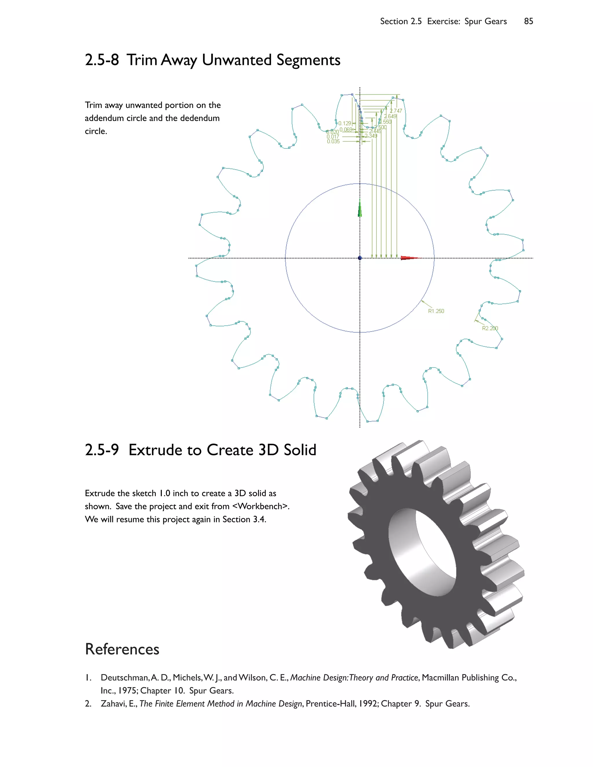
![86 Chapter 2 Sketching
Section 2.6
Exercise: Microgripper
Many manipulators are designed as mechanisms, that is, they consist of bodies connected by joints, such as revolute
joints, sliding joints, etc., and the motions are mostly governed by the laws of rigid body kinematics.
The microgripper discussed here [1-2] is a structure rather than a mechanism; the mobility are provided by the
4exibility of the materials, rather than the joints.
The microgripper is made of PDMS (polydimethylsiloxane, see Section 1.1-1). The device is actuated by a shape
memory alloy (SMA) actuator [3], of which the motion is caused by temperature change, and the temperature is in
turn controlled by electric current.
2.6-1 About the Microgripper
In the lab, the microgripper is tested by gripping a glass
bead of a diameter of 30 micrometer [4].
In this section, we will create a solid model for the
microgripper. The model will be used for simulation in Section
13.3 to assess the gripping forces on the glass bead under the
actuation of SMA actuator.
480
144
176
280
400140212
32
92
7747
87
20
R25R45
D30
Unit: m
Thickness: 300 m
[2] Actuation
direction.
[1] Gripping
direction.
[3] SMA
actuator.
[4] Glass
bead.](https://image.slidesharecdn.com/huei-huanglee-finiteelementsimulationswithansysworkbench12-2010-151020015452-lva1-app6892/75/Finite-Element-Simulations-with-ANSYS-Workbench-2012-73-2048.jpg)
![Section 2.6 Exercise: Microgripper 87
2.6-2 Create Half of the Model
Launch <Workbench>. Create a <Geometry> system. Save
the project as "Microgripper." Start up <DesignModeler>.
Select <Micrometer> as length unit. Start to draw sketch on
the XYPlane.
Draw the sketch as shown on the right side [1]. Note
that two of the three circles have equal radii. Trim away
unwanted segments as shown below [2]. Note that we drew
half of the model, due to the symmetry. Extrude the sketch 150
microns both sides of the plane symmetrically (total depth is
300 microns) [3]. Now we have half of the gripper [4].
[1] Before
trimming.
[2] After
trimming.
[3] Extrude
both sides
symmetrically.
[4] Half of
the gripper.](https://image.slidesharecdn.com/huei-huanglee-finiteelementsimulationswithansysworkbench12-2010-151020015452-lva1-app6892/75/Finite-Element-Simulations-with-ANSYS-Workbench-2012-74-2048.jpg)
![88 Chapter 2 Sketching
2.6-2 Mirror Copy the Solid Body
2.6-3 Create the Bead
Create a new sketch on XYPlane and draw a
semicircle as shown [1-4]. Revolve the
sketch 360 degrees to create the glass bead.
Note that the two bodies are treated as two
parts. Rename two bodies [5].
Wrap Up
Close <DesignModeler>, save the project
and exit <Workbench>. We will resume this
project in Section 13.3.
[3] Select the solid
body and click
<Apply>.
[2] The default type
is <Mirror> (mirror
copy).
[6] Click
<Generate>.
[3] Remember to
impose a <Tangent>
constraint here.
[2]
Remember
to close the
sketch by
draw the
vertical line.
[5] Right-click to
rename two bodies.
[4] Select the <YZPlane> in
the model tree and click
<Apply>. If <Apply> doesn't
appear, see next step.
[1] The
semicircle can
be created by
creating a full
circle and then
trim it using
the axis.
[4] Remember to
specify the
dimension.
[5] If <Apply/Cancel> doesn't
appear, clicking the yellow area
will make it appear.
[1] Pull-down-
select <Create/Body
Operation>.](https://image.slidesharecdn.com/huei-huanglee-finiteelementsimulationswithansysworkbench12-2010-151020015452-lva1-app6892/75/Finite-Element-Simulations-with-ANSYS-Workbench-2012-75-2048.jpg)
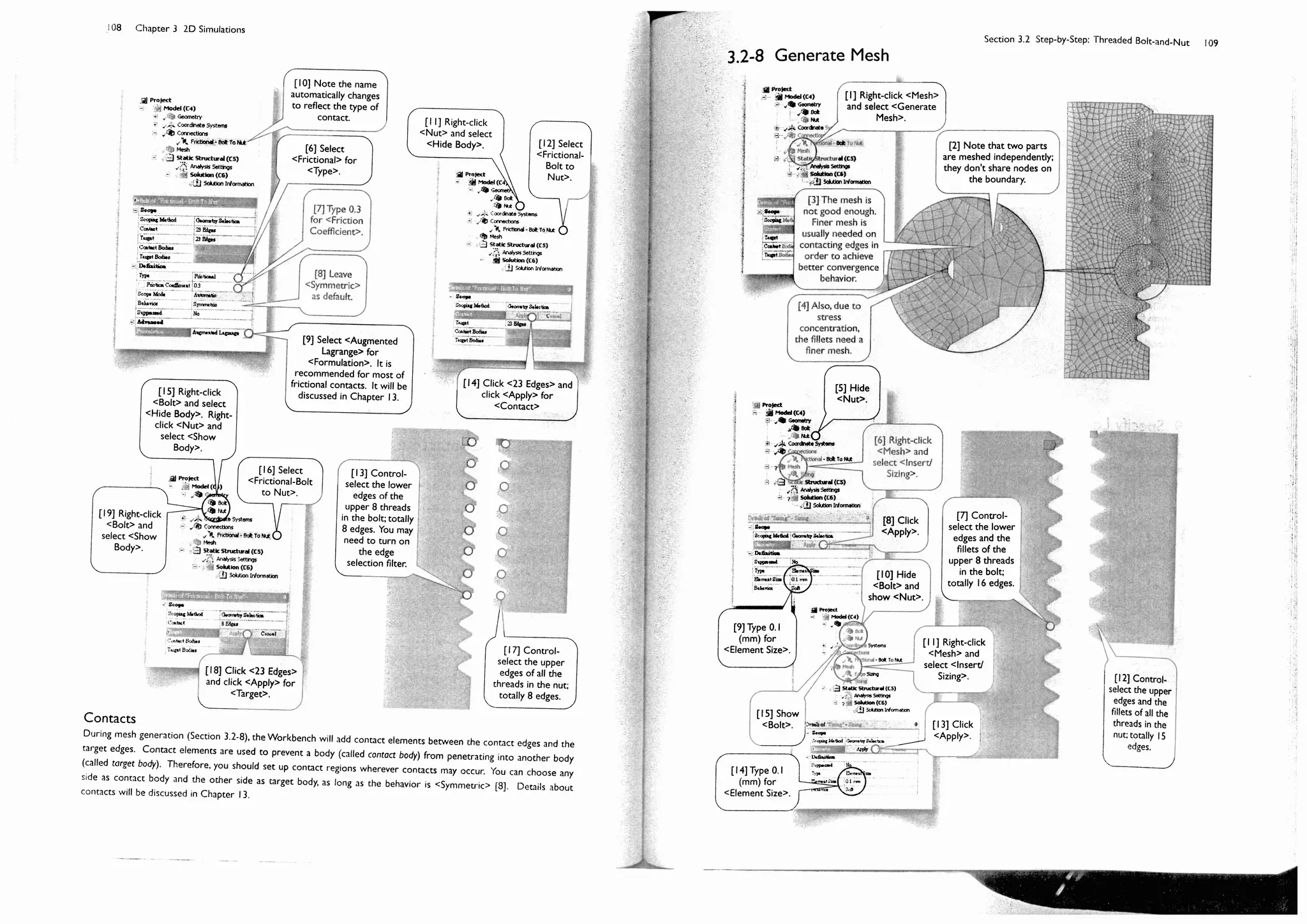
![102 Chapter 3 2D Simulations
Section 3.2
Step-by-Step: Threaded Bolt-and-Nut
3.2-1 About the Threaded Bolt-and-Nut
The plane of symmetry
Theaxisofsymmetry
17 mm
The threaded bolt we created in Section 2.4 is part of a bolt-
nut-plate assembly [1-4]. The bolt is preloaded with a tension.
The pretension is applied by tightening the nut with torque.
The pretension can be calculated by multiplying the maximum
torque with a coefficient, which is empirically determined. The
pretension in our case is 10 kN. We want to know the stress
at the threads under such a pretension condition.
Pretension is a ready-to-use environment condition in
3D simulations, in which a pretension can apply on a body or
cylindrical surface. It is, however, not applicable for 2D
simulations.
In this 2D simulation, we will make some simplification.
Assuming a symmetry between upper and lower part, we
model only upper part of the assembly [5]. The plate is
removed, to reduce the problem size and alleviate the contact
nonlinearity, and its boundary surface with the nut is replaced
by a frictionless support [6].
The pretension is replaced by a uniform force applied on
the lower face of the bolt. The model somewhat deviates
from the reality, which we will discuss at the end of this
section, but for accessing the stress, it should be acceptable.
The coefficient of friction between the bolt and the nut
is estimated to be 0.3.
[1] Bolt. [2] Nut.
[3] Plates.
[4] Section
view.
[5] The 2D
simulation
model.
[6] Frictionless
support.](https://image.slidesharecdn.com/huei-huanglee-finiteelementsimulationswithansysworkbench12-2010-151020015452-lva1-app6892/75/Finite-Element-Simulations-with-ANSYS-Workbench-2012-84-2048.jpg)
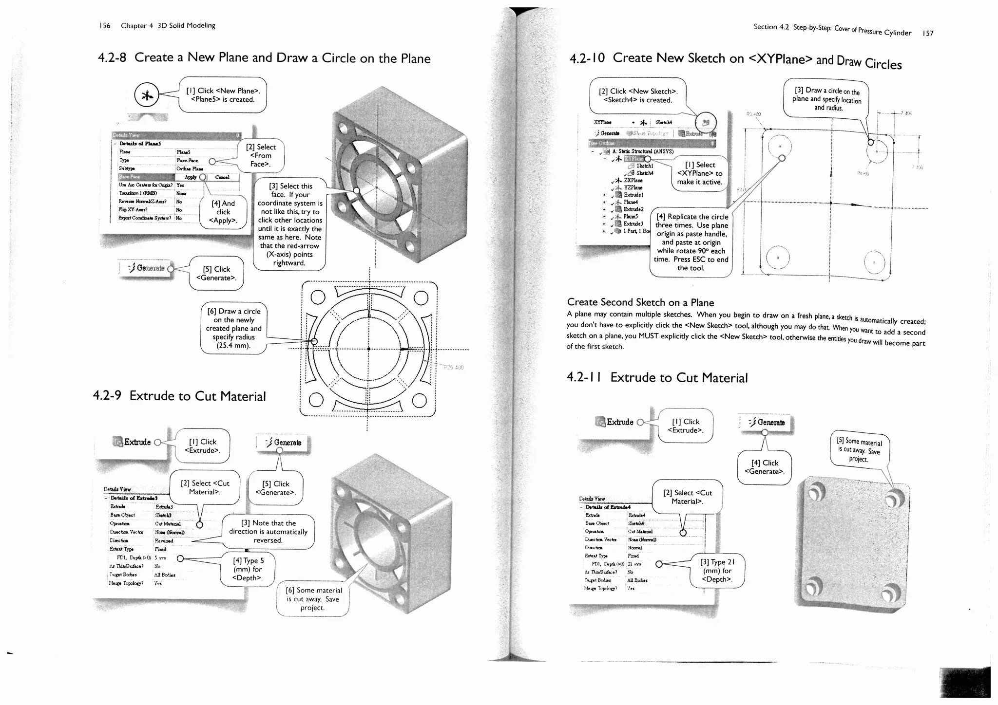
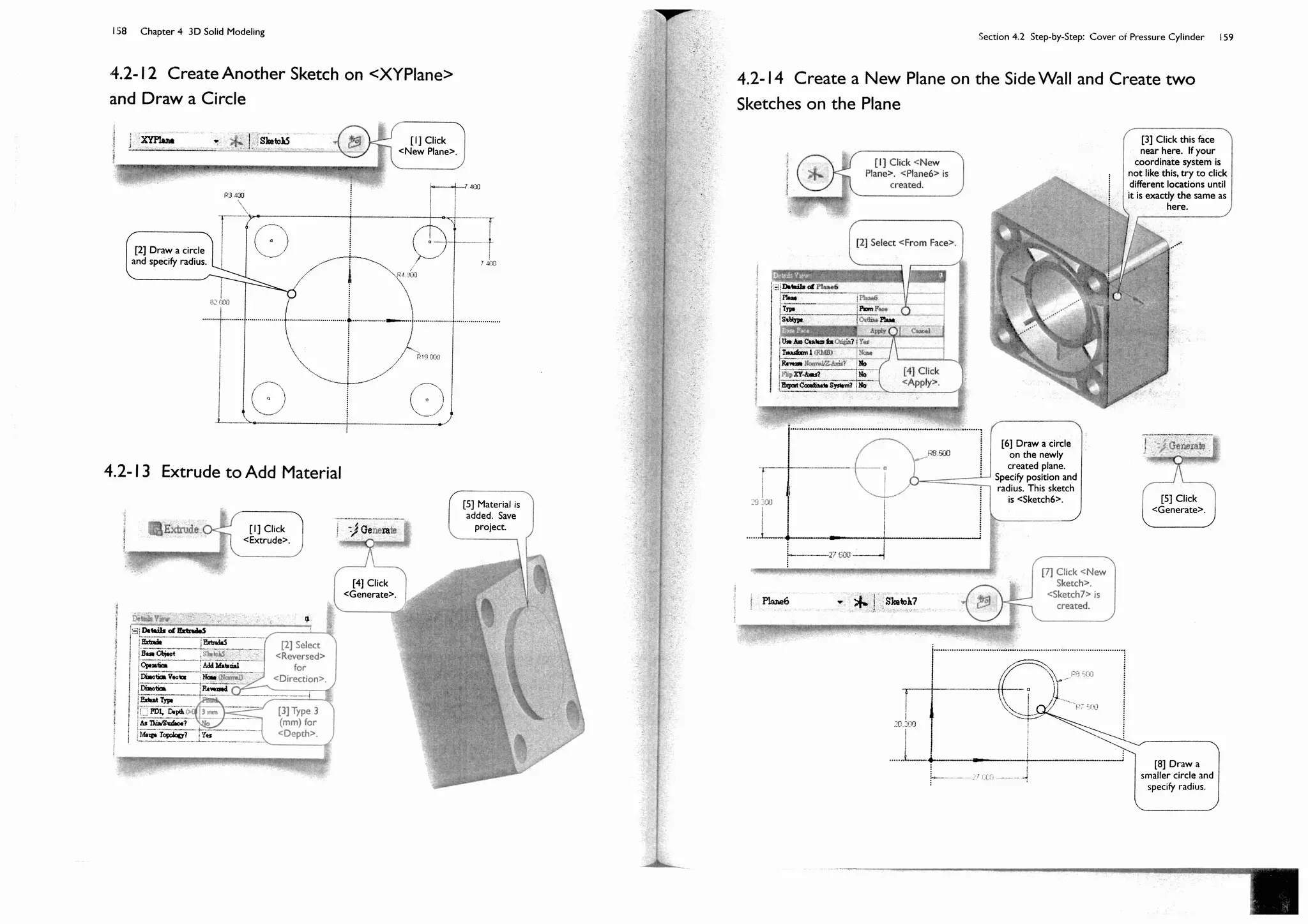
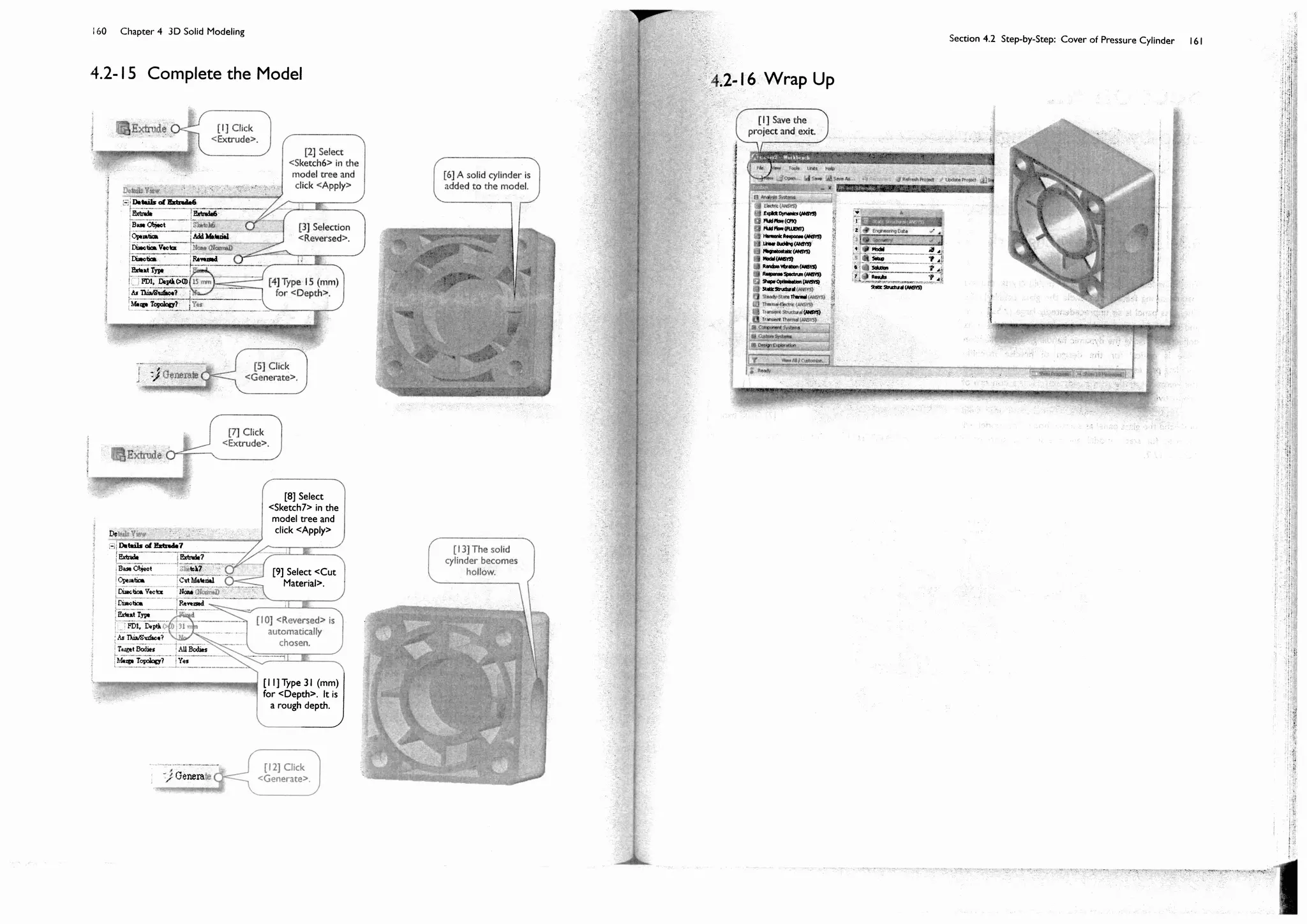
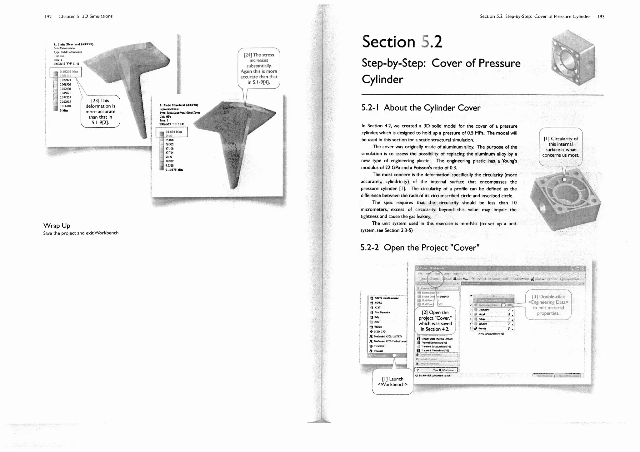
![150 Chapter 4 3D Solid Modeling
Section 4.2
Step-by-Step: Cover of Pressure
Cylinder
4.2-1 About the Cylinder Cover
The pressure cylinder [1] contains gas of 0.5 MPa. The cylinder cover [2-4] is
made of carbon-fiber reinforced plastic. We want to investigate the
deformation of the cylinder cover under such working pressure. We will
create a 3D solid model in this section; the model will be used for a static
structural simulation in Section 5.2.
Unit: mm.
30.3
25.3
21.0 1.3
31.0
3.0
10.0
R8.5
R7.5
R19.0
62.0
2.3 1.6
7.4
7.4
62.0
R4.9
R3.2
R9.0R14.5
R18.1
R25.4
R27.8
R3.4
[1] Pressure
cylinder.
[2] Cylinder
Cover.
[3] A close-up
view of the
cylinder cover.
[4] Back view of
the cover.](https://image.slidesharecdn.com/huei-huanglee-finiteelementsimulationswithansysworkbench12-2010-151020015452-lva1-app6892/75/Finite-Element-Simulations-with-ANSYS-Workbench-2012-109-2048.jpg)
![Section 4.5 Exercise: LCD Display Support 175
Section 4.5
Exercise: LCD Display Support
The LCD Display support is made of an ABS (acrylonitrile-
butadiene-styrene) plastic. The thickness of the plastic is 3
mm [1]. Details of the hinge design is not shown in the figure
but will be shown in 4.5-4 [2].
The solid model will be used in Section 5.4 for a static
structural simulation to assess the deformation and stress
under a design load.
4.5-1 About the LCD Display Support
200
90
60
44
105042
20
17
Unit: mm
[1] The
thickness of the
plastic is 3 mm.
[2] Details of the
hinge design will be
shown in 4.5-4.](https://image.slidesharecdn.com/huei-huanglee-finiteelementsimulationswithansysworkbench12-2010-151020015452-lva1-app6892/75/Finite-Element-Simulations-with-ANSYS-Workbench-2012-123-2048.jpg)

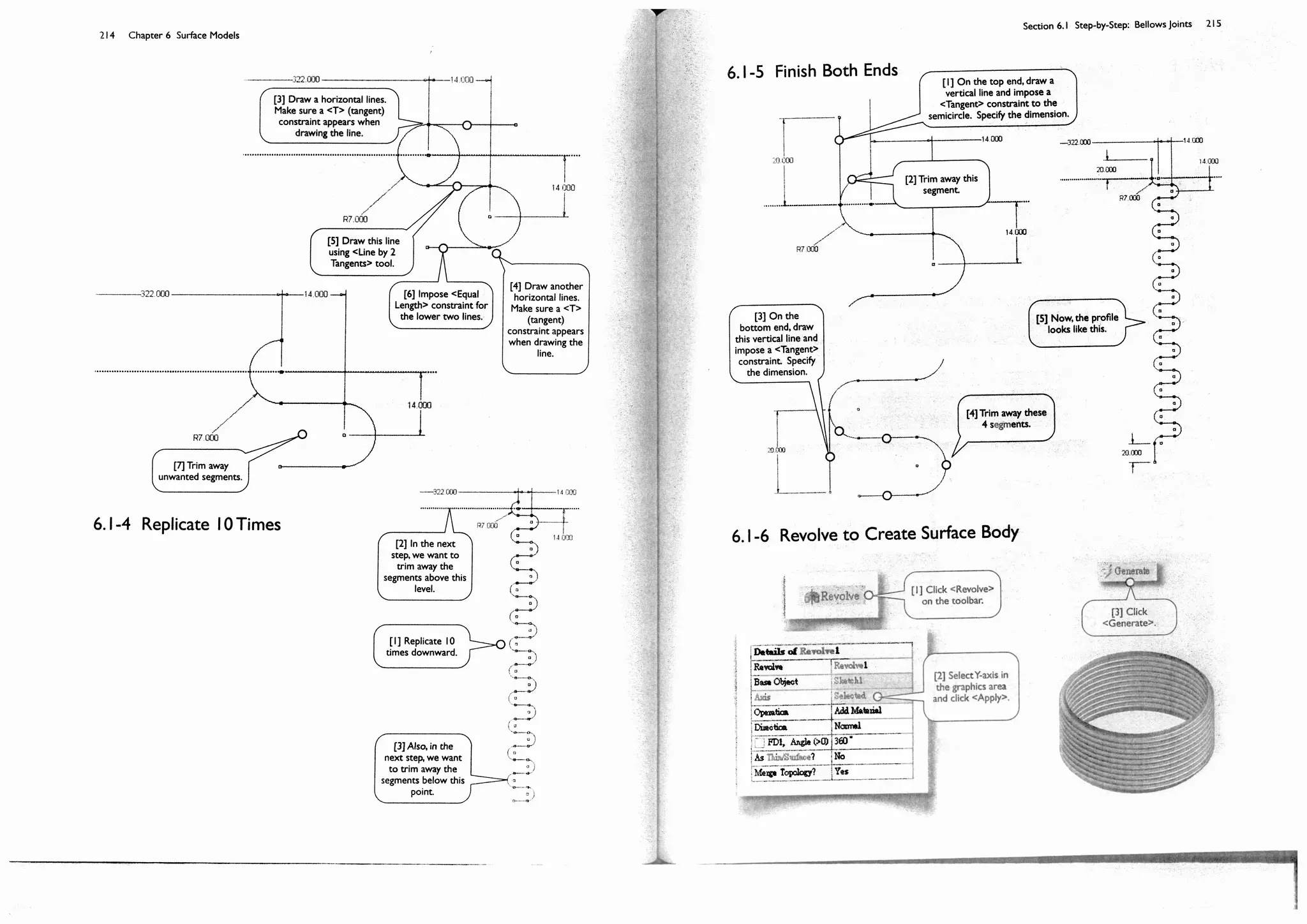
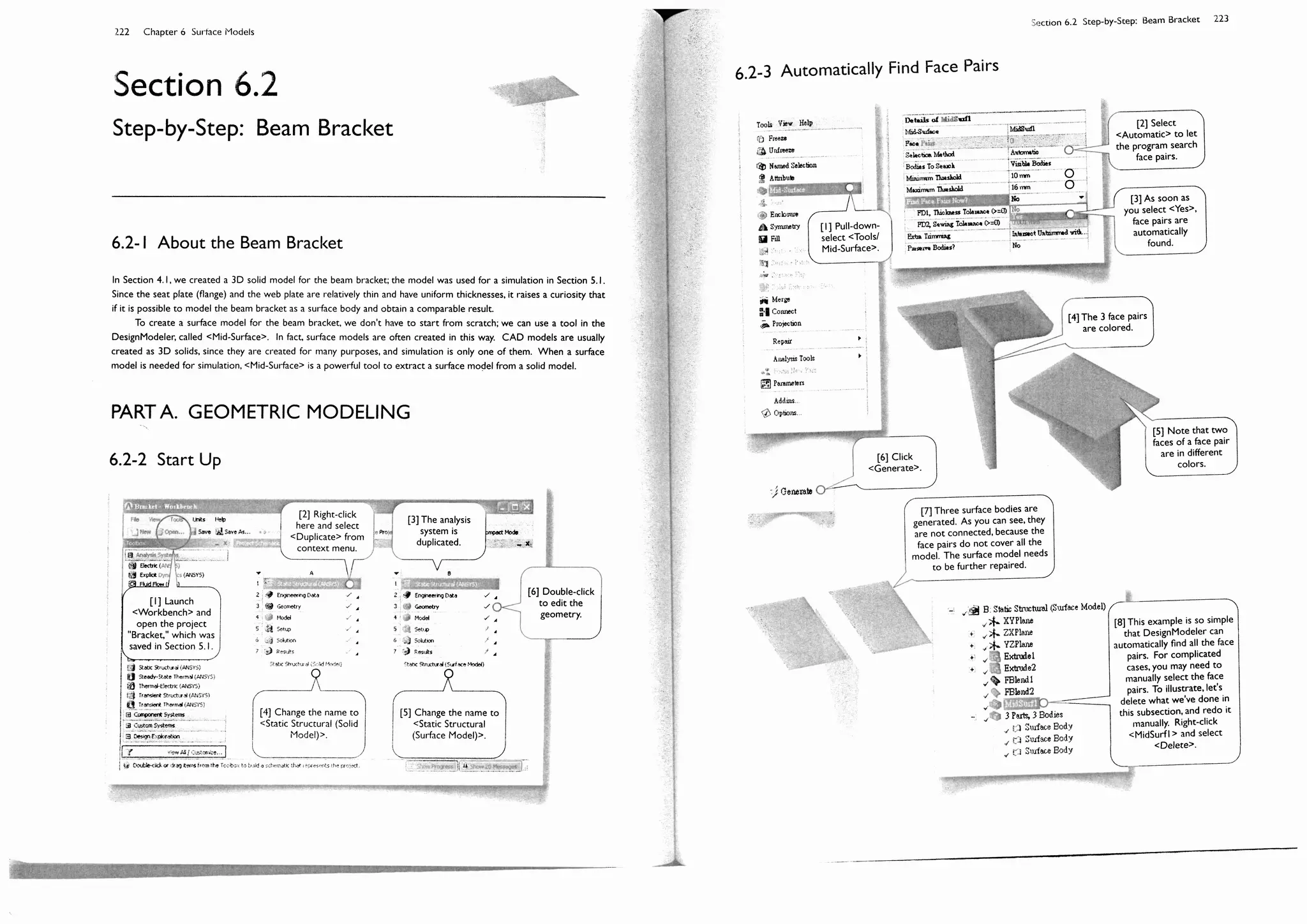
![212 Chapter 6 Surface Models
Section 6.1
Step-by-Step: Bellows Joints
The bellows joints [1-2] are used as expansion joints, which absorb thermal or vibrational movement in a piping
system that transports high pressure gases. As part of the piping system, the bellows joints are designed to sustain
internal pressure as well as external pressure. The external pressure must be considered when the piping system is
used across the ocean. Under the internal pressure, the engineers mostly concern about its radial deformation (due
to an engineering tolerance consideration) and hoop stress (due to the safety consideration). Under the external
pressure, buckling is the main concern (see an exercise in Section 10.4-2).
6.1-1 About Bellows Joints
In this section, we will create a full 3D surface
model for the bellows joint and perform a static
structural simulation under the internal pressure of 0.5
MPa. A buckling simulation under the external pressure
will be left as an exercise in Section 10.4-2.
Note that the problem is axisymmetric both in
geometry and loading. We could take advantage of this
property and model the problem as 2D solid body or 2D
line body (both as axisymmetric models). The latter, 2D
line model, is not supported in the current version of
<Mechanical> (it is supported through APDL). The
former, 2D solid model, usually results a poorer solution
than surface body, for this particular case, because the
bending dominates its structural behavior.
R315
28
R315 28
20
Unit: mm.
[1] The bellows
joints are made of
SU316 steel, which
has aYoung's
modulus of 180
GPa and Poisson's
ratio of 0.28.
[2] All arcs have radii
of 7 mm. The
thickness is 0.8 mm.](https://image.slidesharecdn.com/huei-huanglee-finiteelementsimulationswithansysworkbench12-2010-151020015452-lva1-app6892/75/Finite-Element-Simulations-with-ANSYS-Workbench-2012-142-2048.jpg)


![Section 11.4 Exercise: Guitar String 395
Section 11.4
Exercise: Guitar String
The guitar string in our case is made of steel, which has a mass density of 7850 kg/m3, a Young's modulus of 200 GPa,
and a Poisson's ratio of 0.3. It has a circular cross section of diameter 0.28 mm and a length of 1.0 m. The string is
stretched with a tension T, and is in tune with a standard A note (la), which has been defined to be exactly 440 Hz in
the modern music. In the next subsection (11.4-2), we will perform a modal analysis to find the required tension T.
Before the simulation, let's make some simple calculation. According to the basic physics, the wave traveling on a
string has a speed of
v =
T
μ
Where μ is the linear density (kg/m) of the string. The standing wave corresponding to the lowest frequency is called
the first harmonic mode, which has a wavelength of twice the string length (2L). According to the relation between the
velocity, the frequency, and the wavelength
f =
v
=
v
2L
we can estimate the required tension
T = μ 2fL( )
2
= 7850
(0.00028)2
4
2 440 1.0( )
2
= 374.32 N
11.4-1 About the Guitar String
Meanings of sound quality may be different from the points of view between engineers and musicians. This section
tries to build a bridge for the engineers to the territory of music. When designing or improving a musical instrument,
an engineer must know the physics of music. On the other hand, to fully appreciate the theory of music, a musician
needs to know the physics behind the music.
We will use a guitar string to demonstrate some of the physics of music in this section and Section 12.5. For
those students who are not interested in music theory at all, you can read only the first two subsections (11.4-1 and
11.4-2) and skip the rest of this section. On the other hand, if you want to introduce this article to a friend who does
not have enough background in modal analyses, he can skip the first two subsections and jump to 11.4-3 directly.
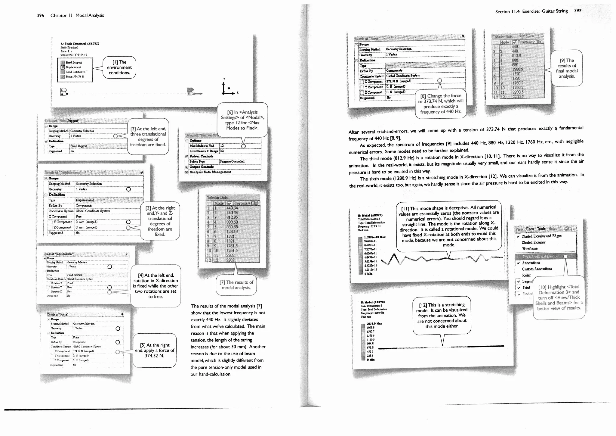
11.4-2 Perform Modal Analysis
Launch the Workbench. Create a <Static Structural> System. Save the project as "String." Drag-and-drop a <Modal>
analysis system to the <Solution> cell of the <Static Structural> system. In the <Engineering Data>, make sure the
material properties for the <Structural Steel> are consistent with those of the guitar string.
Enter the DesignModeler (using <Millimeter> as length unit), create a sketch and use the sketch to create a line
body of 1.0 m. Create a circular cross section of radius 0.14 mm, and associate the line body with the cross section.
Before starting up <Mechanical>, don't forget to turn on <Line Bodies> in the <Properties> (7.1-7[2]). In the
<Mechanical>, specify environment conditions under the <Static Structural> [1]: a <Fixed Support> [2], a
<Displacement> [3], a <Fixed Rotation> [4], and a <Force> [5]. Note that we suppressed all rigid body modes.](https://image.slidesharecdn.com/huei-huanglee-finiteelementsimulationswithansysworkbench12-2010-151020015452-lva1-app6892/75/Finite-Element-Simulations-with-ANSYS-Workbench-2012-241-2048.jpg)
![Section 11.4 Exercise: Guitar String 399
11.4-4 Just Tuning System1
Why do some notes sound pleasing to our ears when played together, while others do not? We know from the
experience that when two notes have a simple frequency ratio, they sound harmonious with each other. The simpler
the ratio, the more harmonious it sounds. The details will be explained in Section 11.4-6. For now, we simply believe it.
In Western music, an 8-tone musical scale has traditionally been used. When learning to sing, we identify the eight
tones in the scale by the syllables do, re, mi, fa, sol, la, ti, do. For a C-major scale in a piano, there are 8 white keys from a
C to the higher pitch of C [1]. The two C's has a frequency ratio of 2:1, and are said to be an octave apart. If we play
two notes an octave apart, they sound very similar. In fact, we often have difficulty telling the difference between two
notes having an octave apart. This is because that, except the fundamental harmonic of the lower note, two notes have
most of the same higher harmonics.
For the following discussion, let's arbitrarily assume the frequency of the lower pitch C as 1. (In a modern piano,
the middle C has a frequency of 261.63 Hz; see the table in Section 11.4-5.) Then the frequency of the higher pitch C is
2. Before being replaced by the "equal temperament" (Section 11.4-5) in the early 20th century, the "just tuning"
systems prevail in the music world. In a just tuning music system, the frequencies of the notes between the 2 C's are
chosen according to the "simple ratio" rule, in order to be harmonious to each other. The result is as shown [2]. Note
that we didn't show the frequency ratios for the black keys (the semitones) to simplify our discussion.
Now, you can appreciate that if we play the notes do and sol together, the sound is pleasing to our ears, since they
have the simplest frequency ratio between 1 and 2. You also can appreciate that the major cord C consists of the notes
do, me, sol, do, the simplest frequency ratios (but not too "close," to avoid beats; see Section 11.4-6) between 1 and 2.
The problem of the just tuning system is that it is almost impossible to play in another key. For example, when
we play in D key, then the frequency ratio between D and its fifth (A) is no longer 3/2. Instead, the frequency ratio is an
awkward 40/27; the two notes are not harmonious enough any more.
C D E F G A B C
do re mi fa sol la ti do
C#
D#
F#
G#
A#
C#
Db
Eb
Gb
Ab
Bb
Db
1
9
8
5
4
4
3
3
2
5
3
15
8
2
11.4-5 Twelve-Tone Equally Tempered Tuning System2
Modern Western music is dominated by a 12-tone equally tempered tuning system, or simply equal temperament. The idea
is to compromise on the frequency ratios between the notes, so that they can be played in different keys. In this
system, an octave is equally divided into 12 tones (including semitones) in logarithmic scale. In other words, the
adjacent tones has a frequency ratio of 2112
, or 1.05946. For example, the frequency ratio between the C#
and the C
is 2112
; the frequency ratio between the A and the lower C is 25 12
. According to this idea, frequencies of the notes can
be calculated and listed in the table below. For comparison, we also list the frequencies of the notes in the just tuning
system. The data in the table are plotted into a chart as shown [1, 2]. The compromised frequencies are close enough
to the just tuning system that most of musicians are satisfied with this system for centreis.
[1] There are 8
notes across an
octave.
[2] The frequency
ratios in a "just
tuning" system.](https://image.slidesharecdn.com/huei-huanglee-finiteelementsimulationswithansysworkbench12-2010-151020015452-lva1-app6892/75/Finite-Element-Simulations-with-ANSYS-Workbench-2012-244-2048.jpg)
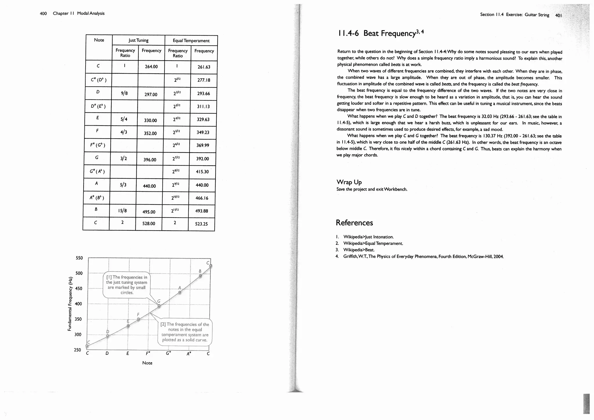
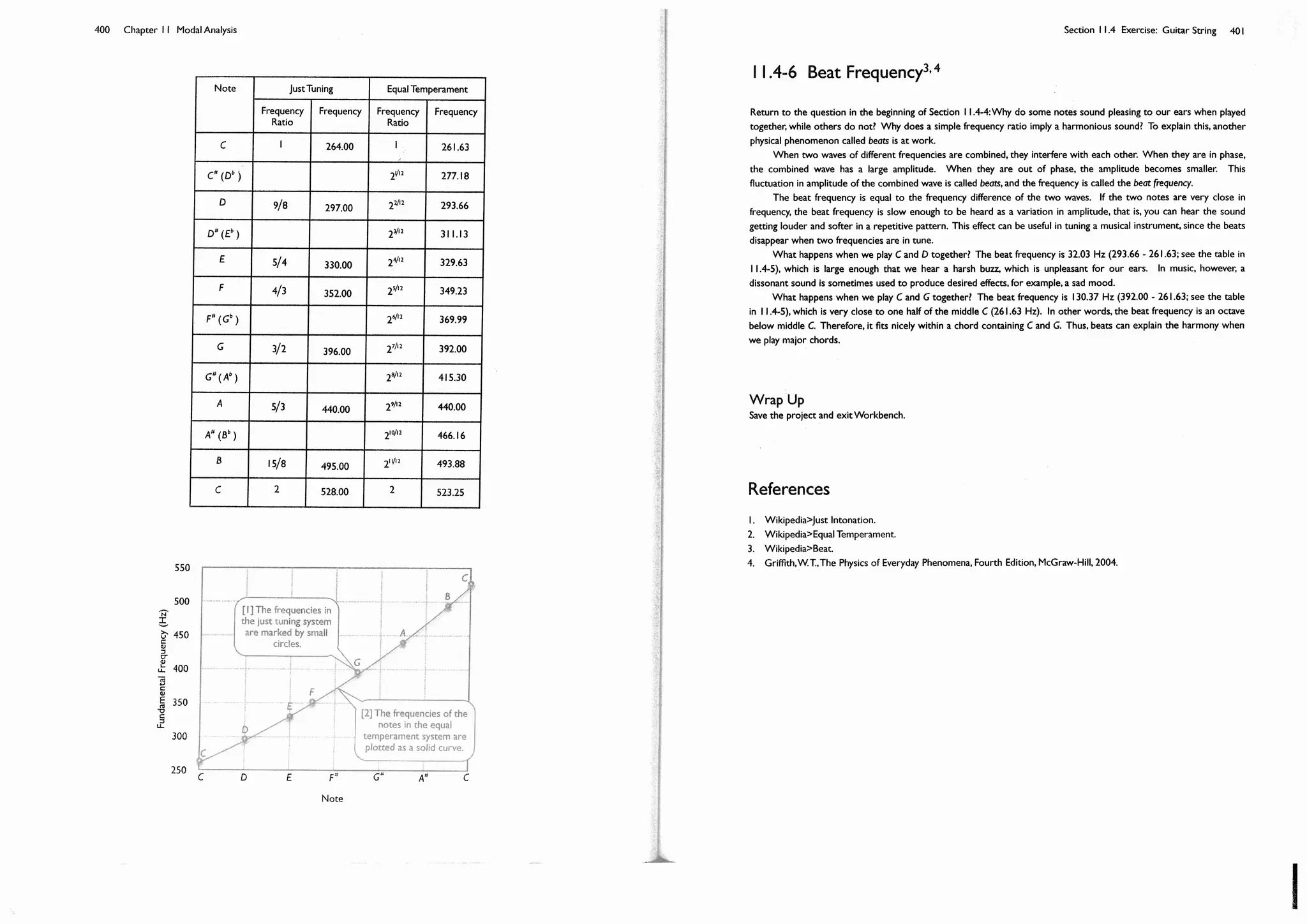
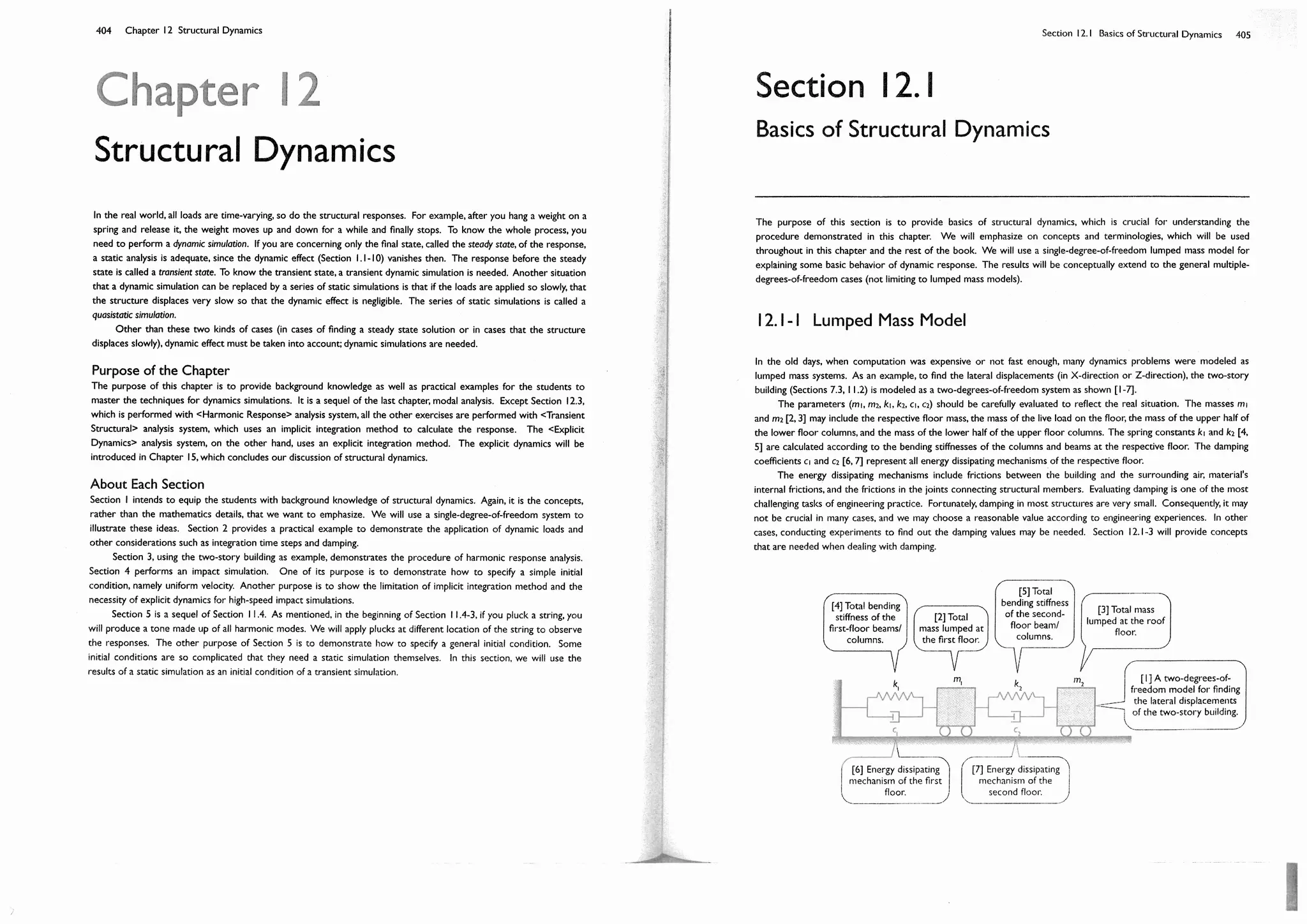
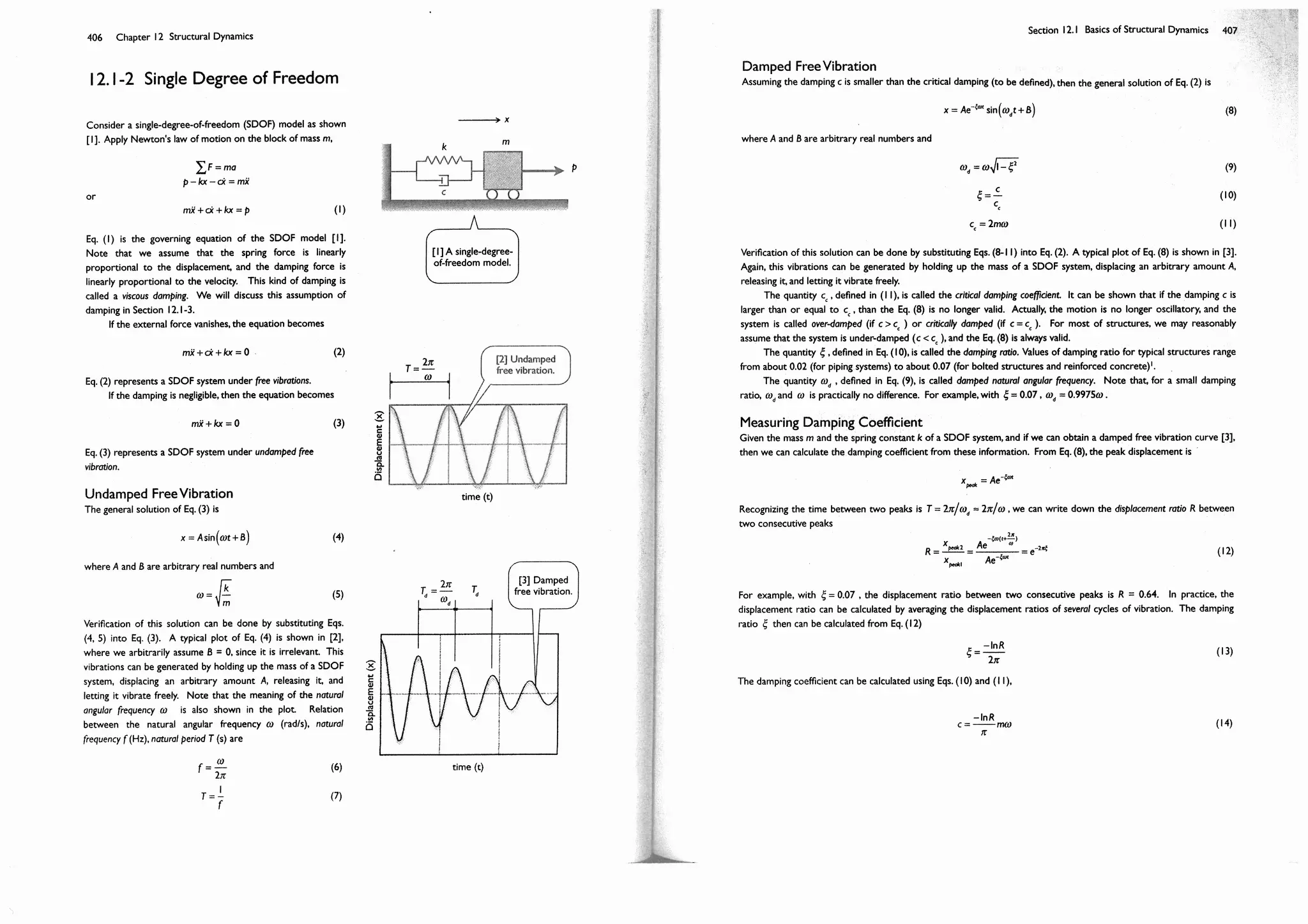
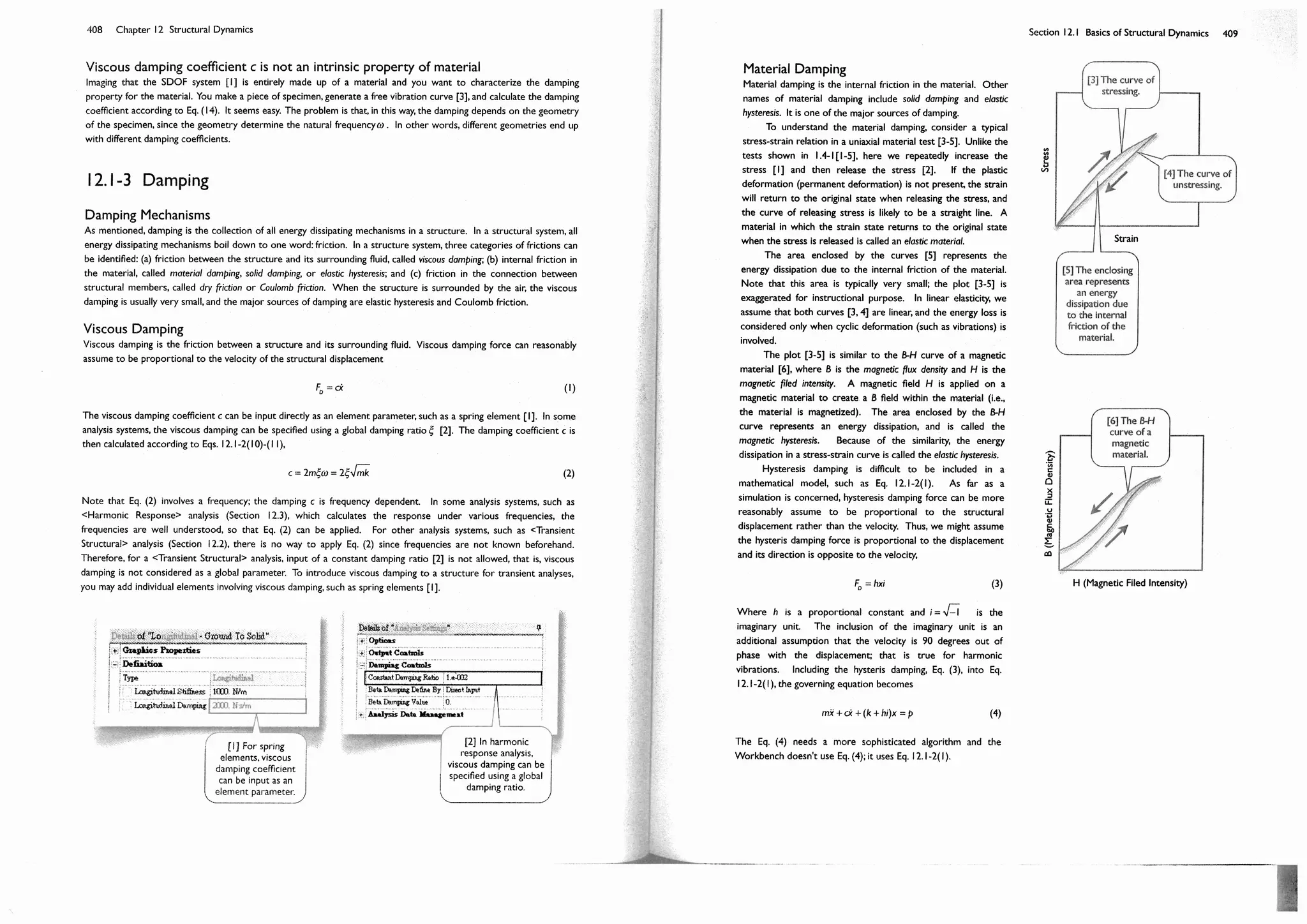
![410 Chapter 12 Structural Dynamics
Recognizing that the damping is small for a structure and the global behavior is similar regardless of the sources
of damping, the Workbench assumes that the hysteris damping force is proportional to the velocity of the structural
displacement, the same as the viscous damping,
FD
= cx (5)
However, we cannot characterize a material using a damping coefficient c. As mentioned in the end of Section 12.1-2,
the damping coefficient c is not an intrinsic property of a material. To filter out other factors, such as geometry, we
need more elaboration. Eq. (2) shows how the coefficient c relates to the mass m and stiffness k for the case of single
degree of freedom; for cases of multiple degrees of freedom, the relation is not so simple. In engineering practice, an
efficient way to characterize a material is proposing a mathematics form with parameters and then determining the
parameters using data fitting. We assume that the coefficient c is a linear combination of the mass m and the stiffness
k, that is,
c = m + k (6)
Now, the parameters and are used to characterize the damping property of a material. The students may
wonder why don't we just assume c = mk , which would be closer to the form of Eq. (2), and characterize the
material by a single parameter . The reason is that, in general, we are dealing with multiple degrees of freedom
system, where m and k are matrices, and the simple relation of Eq. (2) doesn't exist.
Using c = 2m in Eq. (2) and k = m 2
in Eq. 12.1-2(5), Eq. (6) can be rewritten in terms of frequency and
damping ratio,
2 = + 2
(7)
If we can make a single material specimen and measure the damping ratios i
under different excitation frequencies
i
, or make several material specimens of different sizes, and measure the damping ratios i
under their respective
fundamental frequencies i
, or a combination of the above ideas, then we can evaluate the material parameters and
by a standard data fitting procedure.
In the core of ANSYS, it does implement the idea of Eq. (6). Using the APDL commands2, you can input a global
value (using ALPHAD command) and a global value (using BETAD command). You also can input value for
each material as its property (using MP, DAMP).
In the current version of Workbench, you cannot input a global value (it assumes = 0 ), but it allows you to
input a global value [7]. It also allows you to input a value for each material as a material property [8, 9].
[7] A global beta
value can be input
here.
[8] Beta value as a
material property
can be included.
[9] When included,
the beta value of the
material can be input
here.](https://image.slidesharecdn.com/huei-huanglee-finiteelementsimulationswithansysworkbench12-2010-151020015452-lva1-app6892/75/Finite-Element-Simulations-with-ANSYS-Workbench-2012-251-2048.jpg)
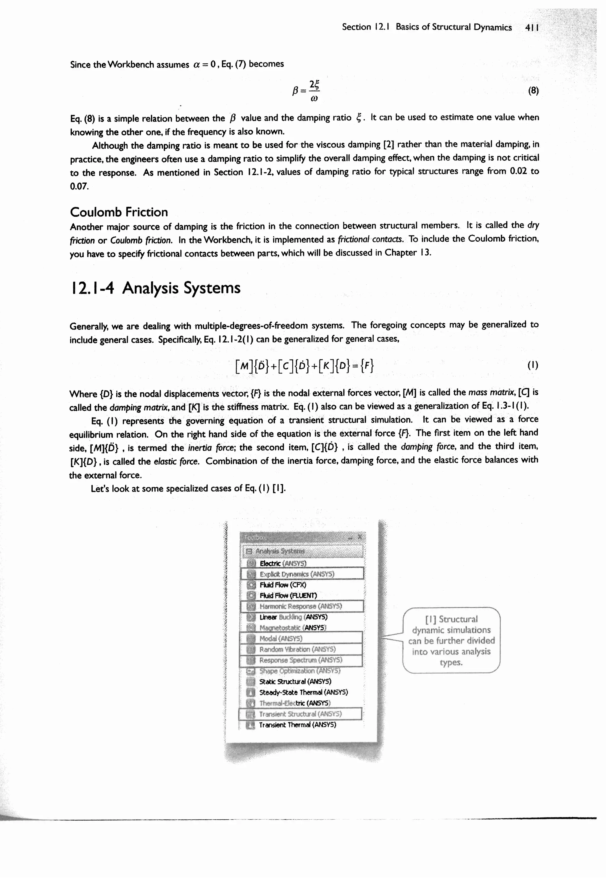
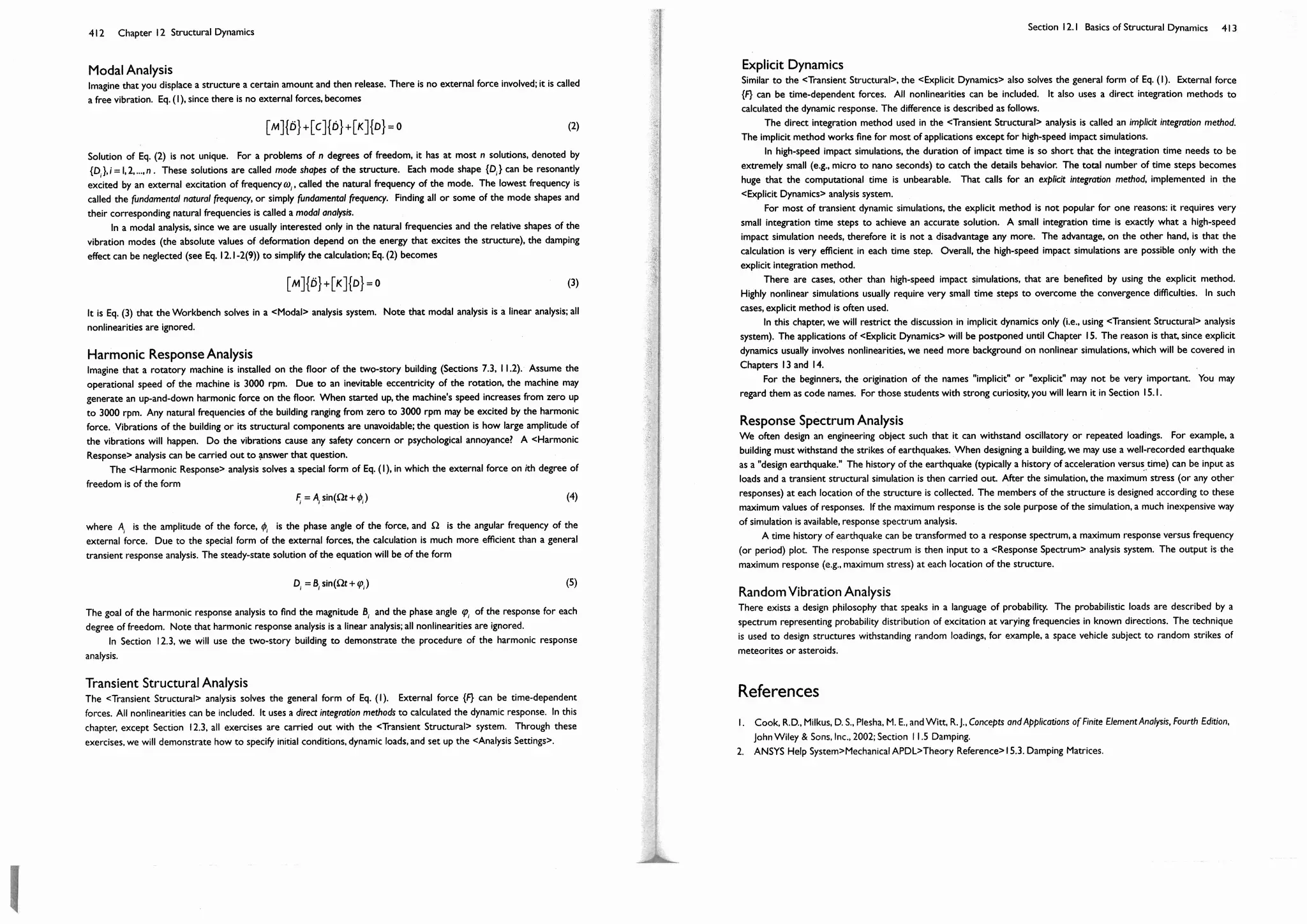
![414 Chapter 12 Structural Dynamics
Section 12.2
Step-by-Step: Lifting Fork
In Section 4.3, we built a model for a lifting fork and glass. The lifting fork [1] is used in an LCD factory to handle the
glass panel [2]. The fork is modeled as solid body and the glass as surface body. The glass panel is so unprecedentedly
large that the engineers concern about its vertical deflections during the dynamic handling.
The fork is made of steel with a density of 7850 kg/m3,Young's modulus of 200 GPa, and Poisson's ratio of 0.3.
The glass has a density of 2370 kg/m3,Young's modulus of 70 GPa, and Poisson's ratio of 0.22.
In this section we will perform a static structural simulation first, to evaluate the vertical deflection of the glass
panel under the gravitational force. This is a critical when determining the clearance of the processing machine [3].
During the dynamic handling, the fork accelerates upward to 6 m/s in 0.3 second and then decelerates to stop in
another 0.3 second, causing the glass panel vibrate [4]. We want to know the time duration when the vibration is
settled to a certain amount so that the glass can be pushed into the processing machine [3]. We also want to know
the maximum stress during the handling. Before the simulation of the dynamic handling, we will perform a modal
analysis to obtain the vibration frequency of the system. This frequency will help us estimate the initial integration
time step.
12.2-1 About the Lifting Fork
12.2-2 Resume the Project "Fork"
Launch <Workbench>. Open the project
"Fork," saved in Section 4.3.
[1] The lifting
fork.
[2] The glass
panel.
[3] Schematic
of the
processing
machine.
[1] Double-click to
start up
<Engineering Data>.
[4] During the
handling, the fork
accelerates upward
to a velocity of 6 m/s
in 0.3 second, and
then decelerates to
a stop in another 0.3
second, causing the
glass panel vibrate.](https://image.slidesharecdn.com/huei-huanglee-finiteelementsimulationswithansysworkbench12-2010-151020015452-lva1-app6892/75/Finite-Element-Simulations-with-ANSYS-Workbench-2012-254-2048.jpg)
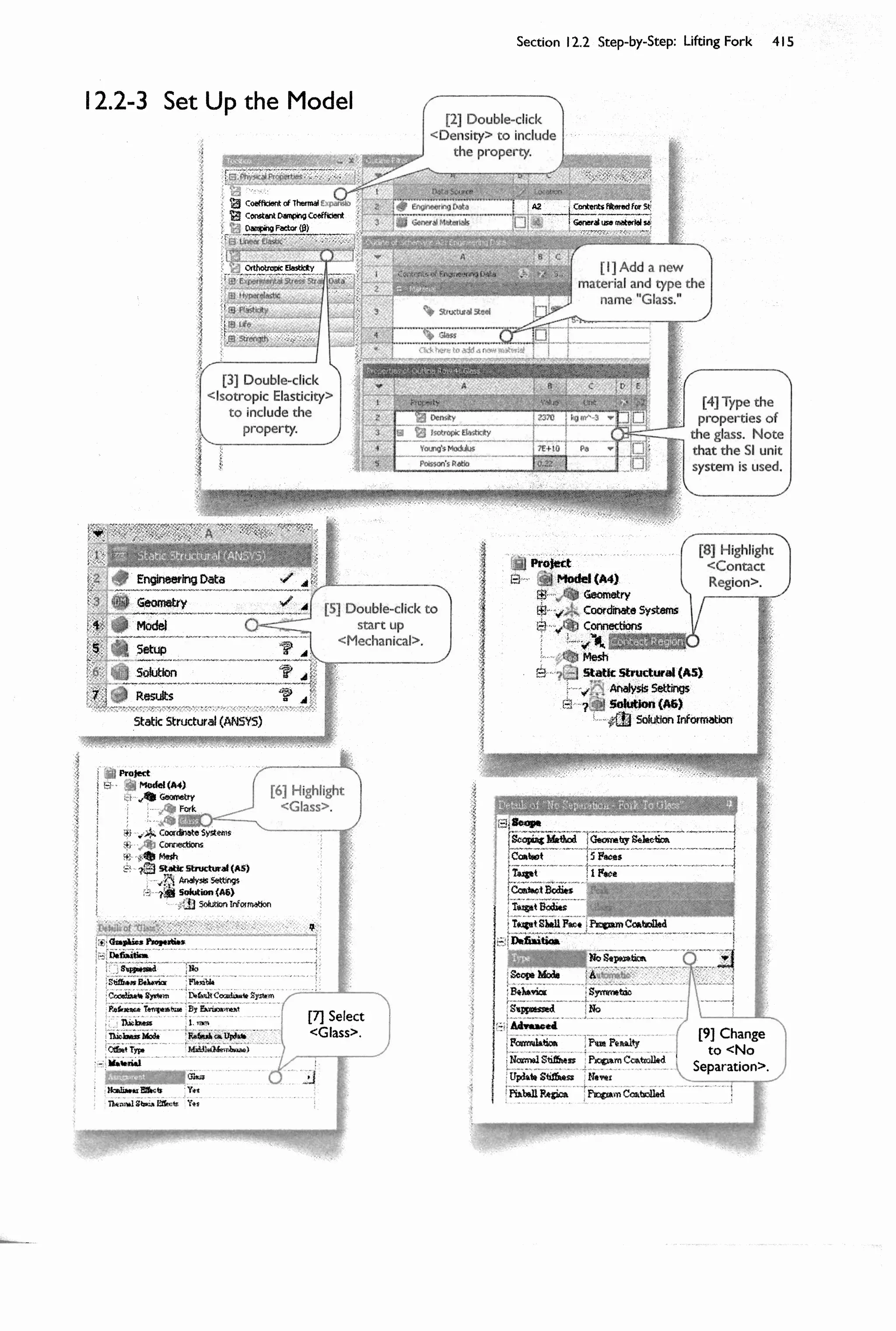
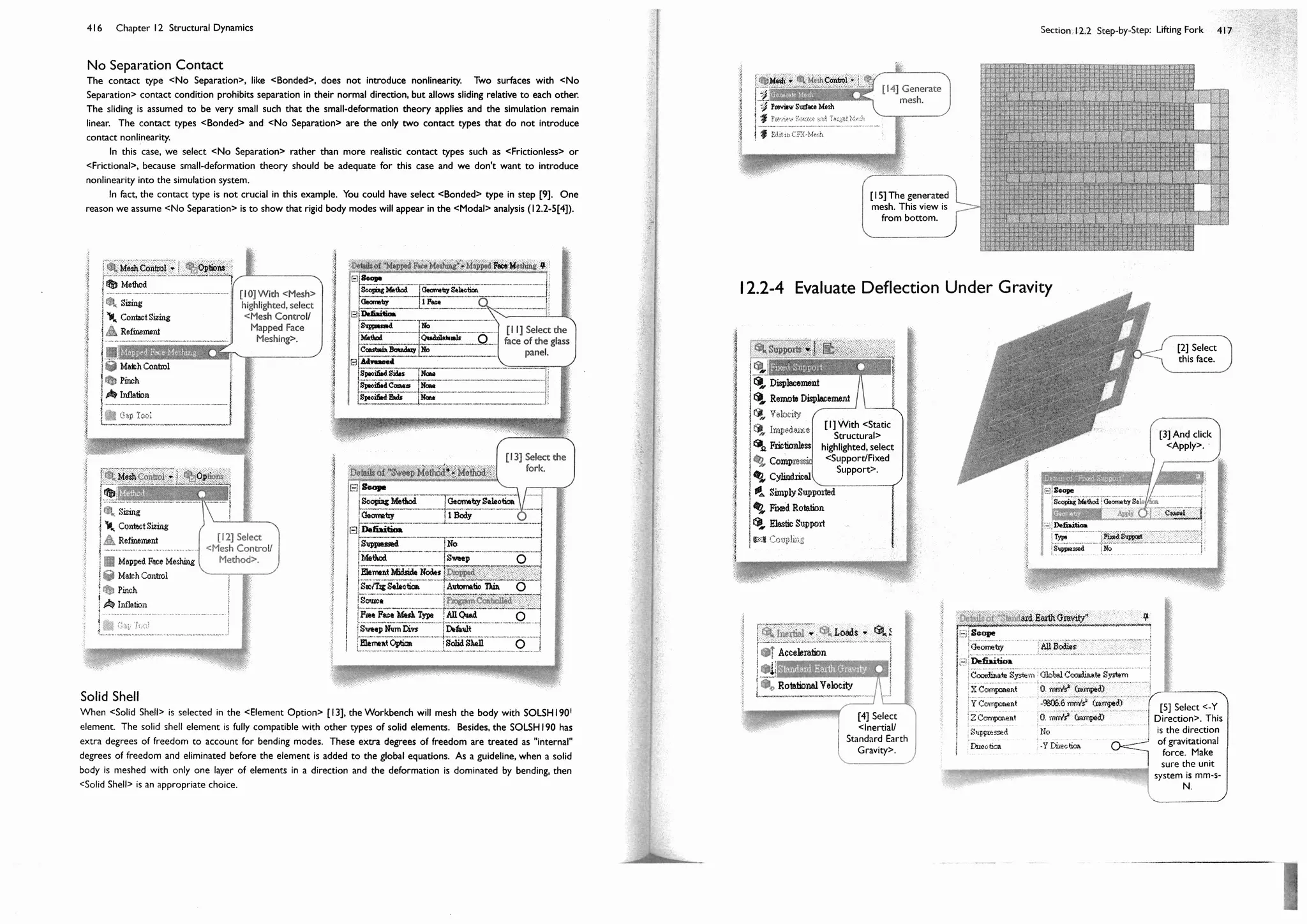
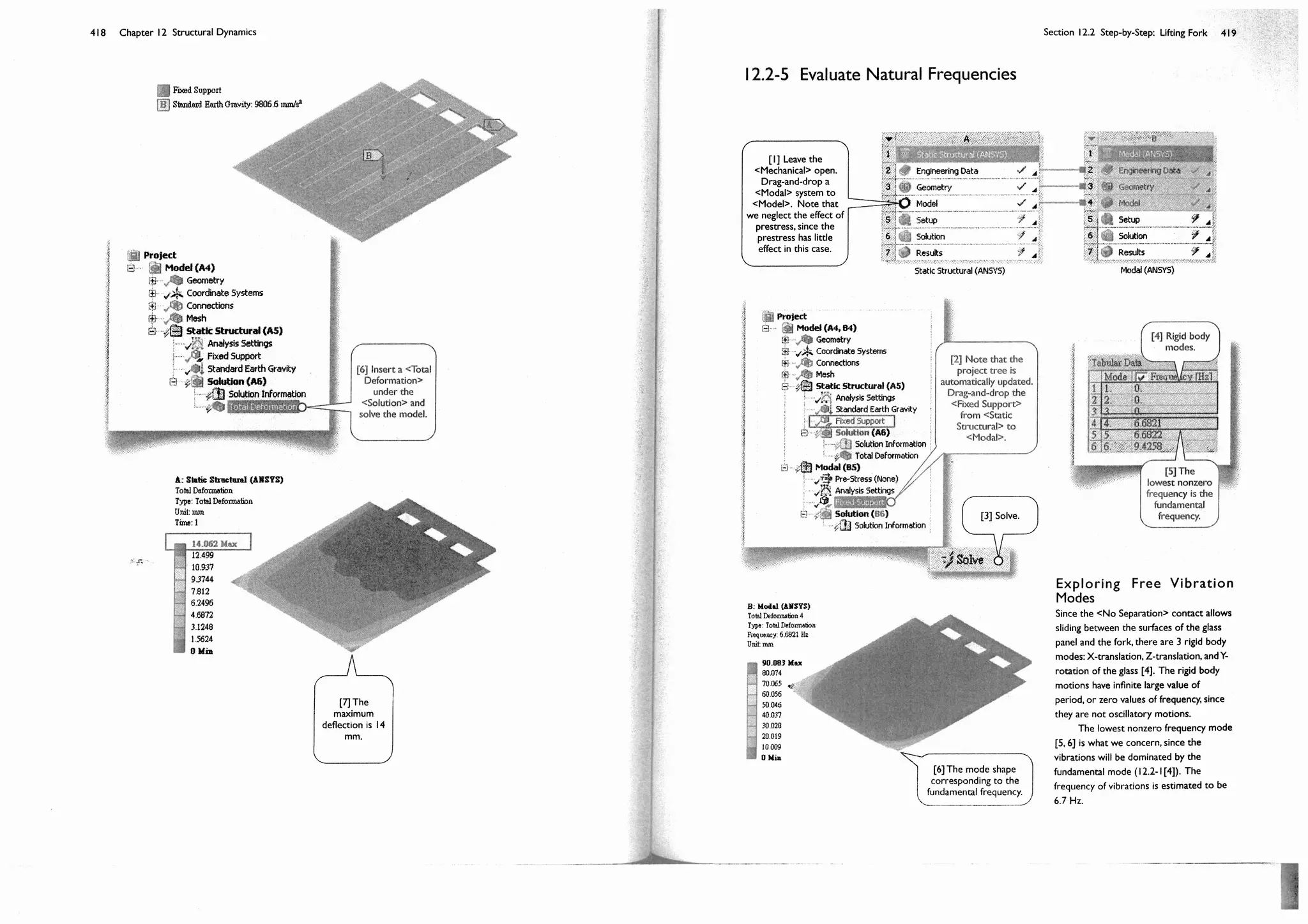
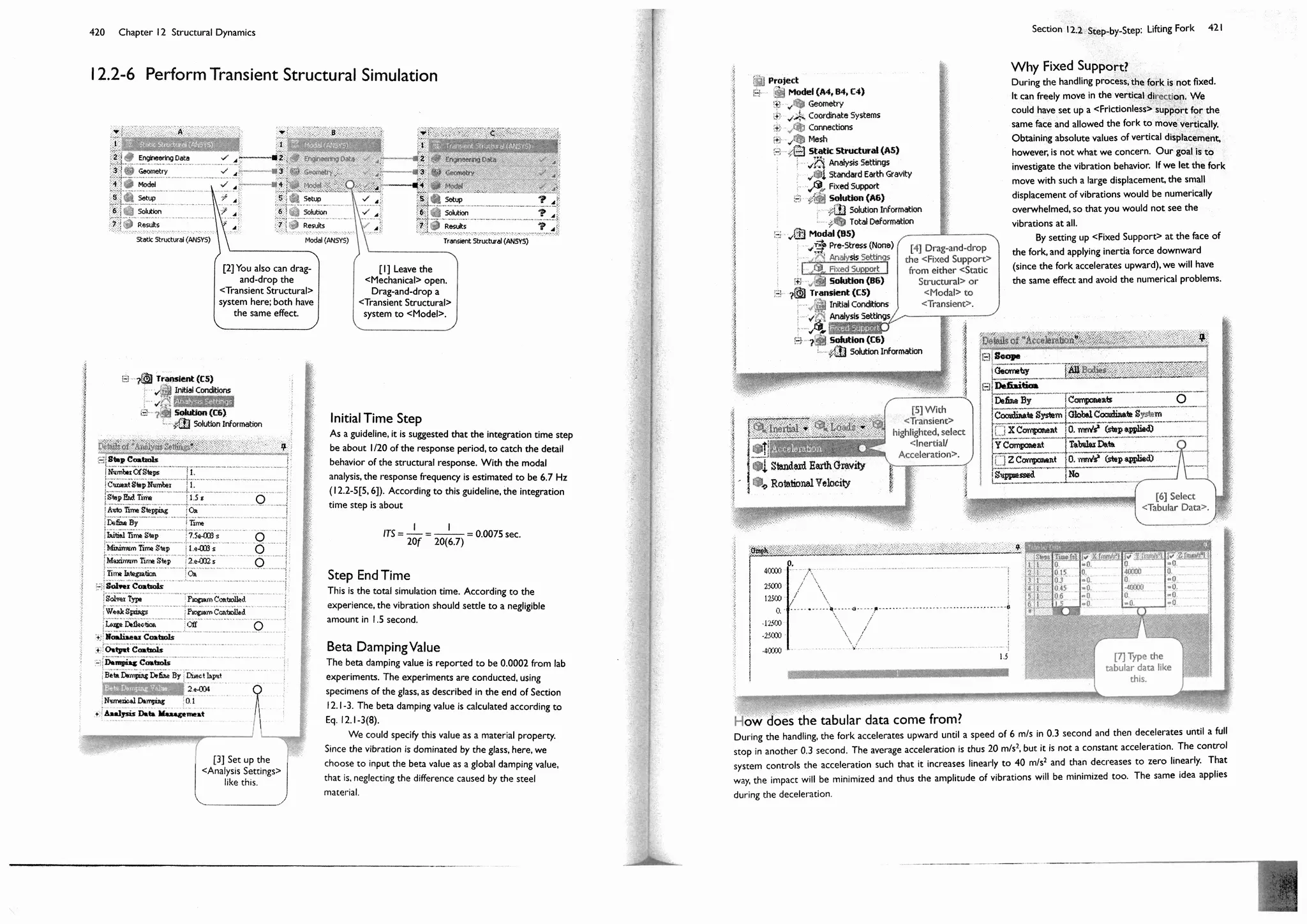
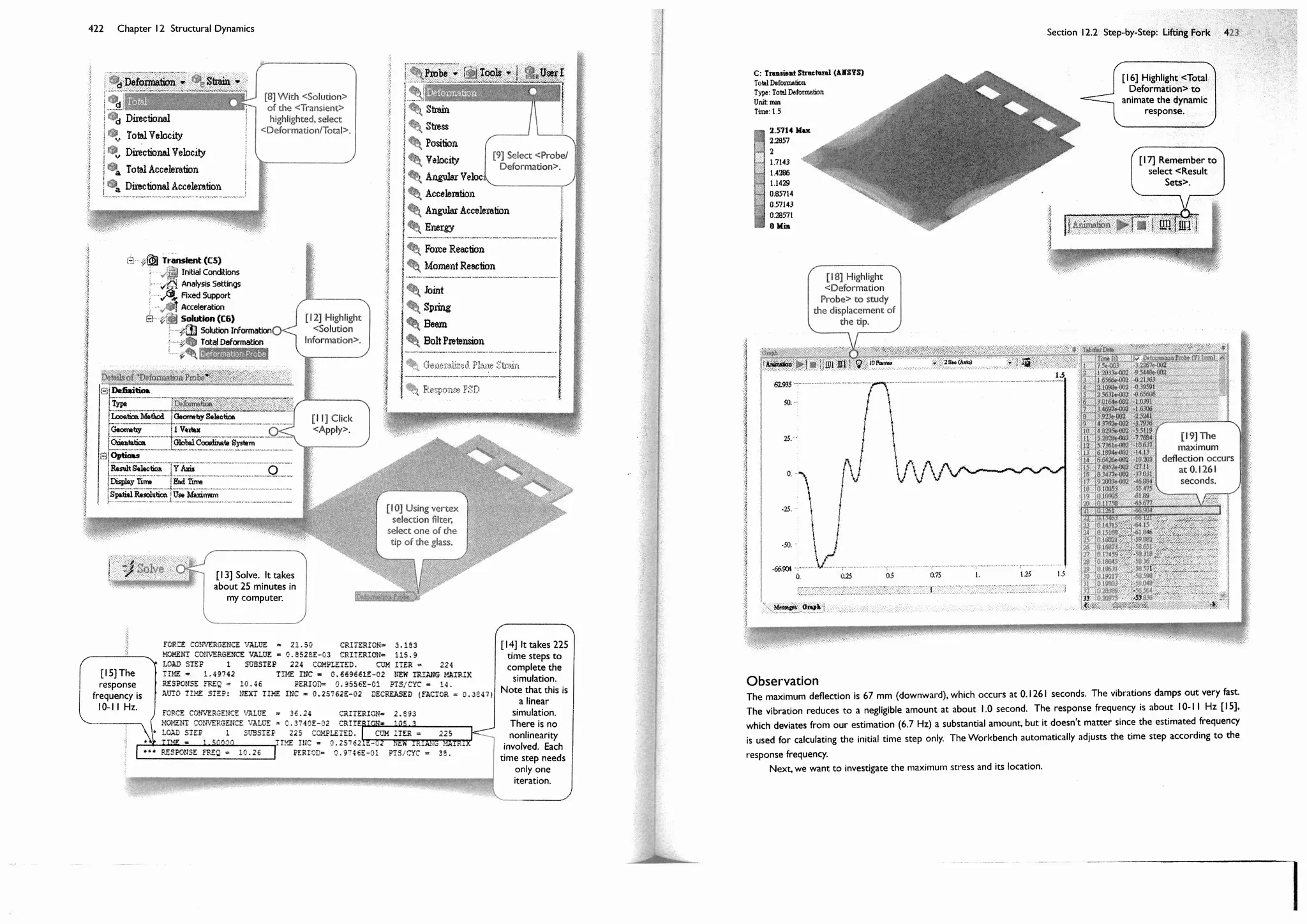
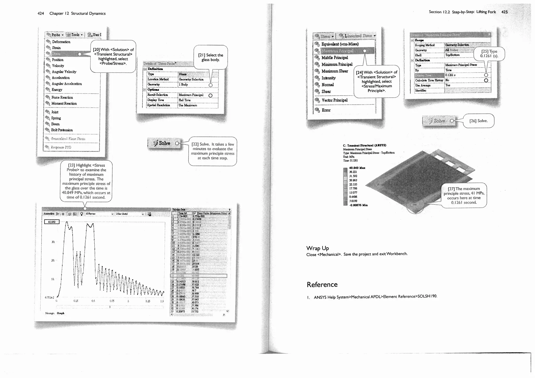
![426 Chapter 12 Structural Dynamics
Section 12.3
Step-by-Step: Two-Story Building
In this section, we will demonstrate the procedure of a harmonic response analysis. The two-story building (Sections
7.3, 11.2) will be used to demonstrate the procedures.
Harmonic Response Analysis
At the end of Section 11.2-3, we mentioned that the rhythmic loading on the floor may cause a safety issue. Is
"dancing on the floor" really an issue? Since the building is designed to withstand a live load of 50 psf (lb/ft2), we will
assume that a group of young people of 50 psf is dancing on a side-span floor deck [1] to simulate an asymmetric
loading that will cause the building side sway. The dancing is so hard that the young people generate a vertical
harmonic force of 10 psf, that is, the loading fluctuates from 40 psf to 60 psf.
Engineers usually don't consider "dancing" as a serious issue. Let's look at a more realistic engineering
consideration. Imagine that an electric motor or any rotatory machine is installed on the floor deck [1]. The
operational speed of the machine is 3000 rpm. When started up, the machine's speed increases from zero up to 3000
rpm. Are the vibrations caused by the rotatory machine an issue? In this section, we will perform a harmonic
response analysis to answer the above questions.
12.3-1 About the Two-Story Building
12.3-2 Perform an Unprestressed Modal Analysis
Launch <Workbench>. Open the project "Building," saved in Section 11.2.
[1] Harmonic
loading will apply
on this floor
deck.
[1] In this section,
we want to reuse this
system. Remember
the model in this
system has no diagonal
members.](https://image.slidesharecdn.com/huei-huanglee-finiteelementsimulationswithansysworkbench12-2010-151020015452-lva1-app6892/75/Finite-Element-Simulations-with-ANSYS-Workbench-2012-261-2048.jpg)
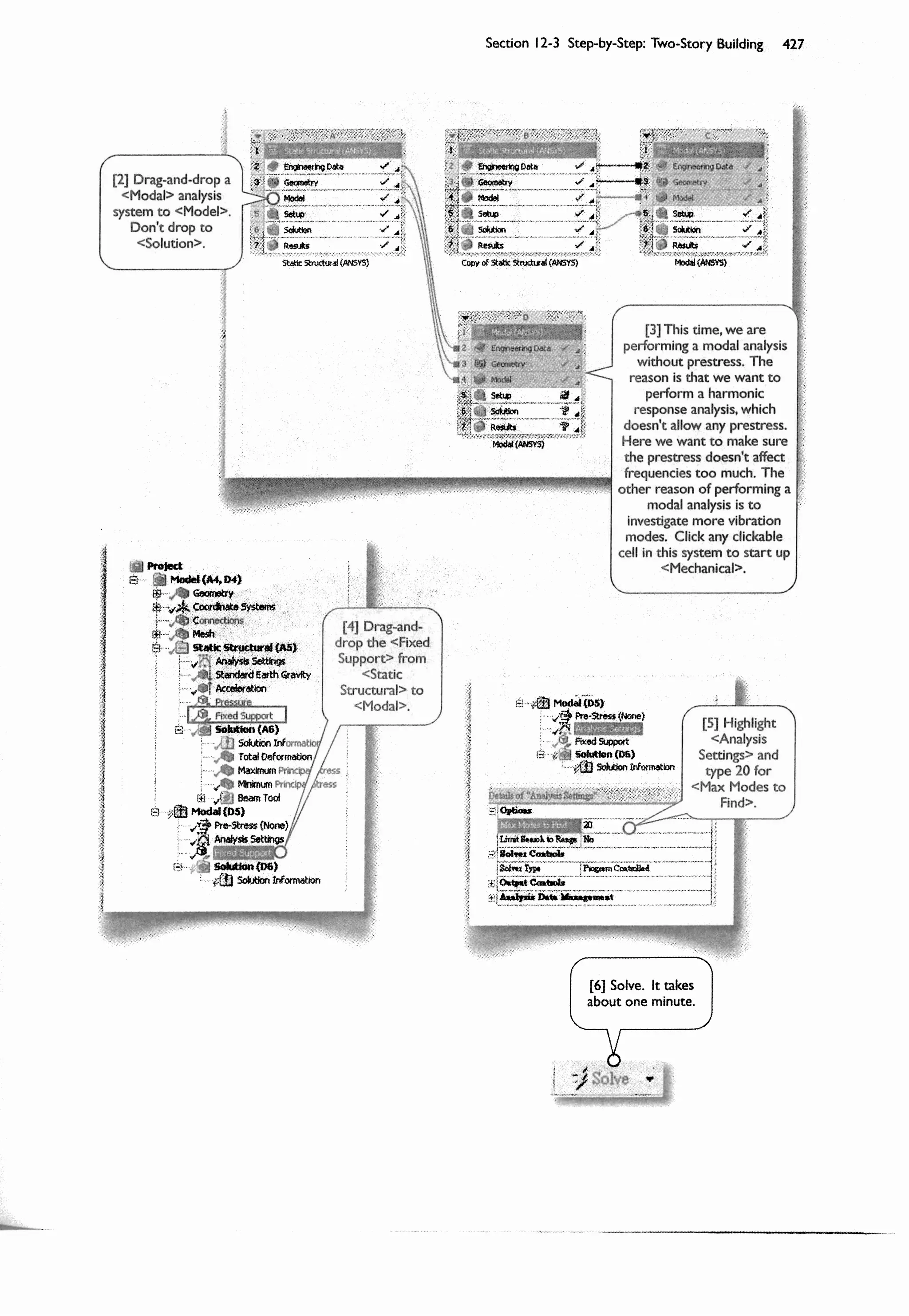
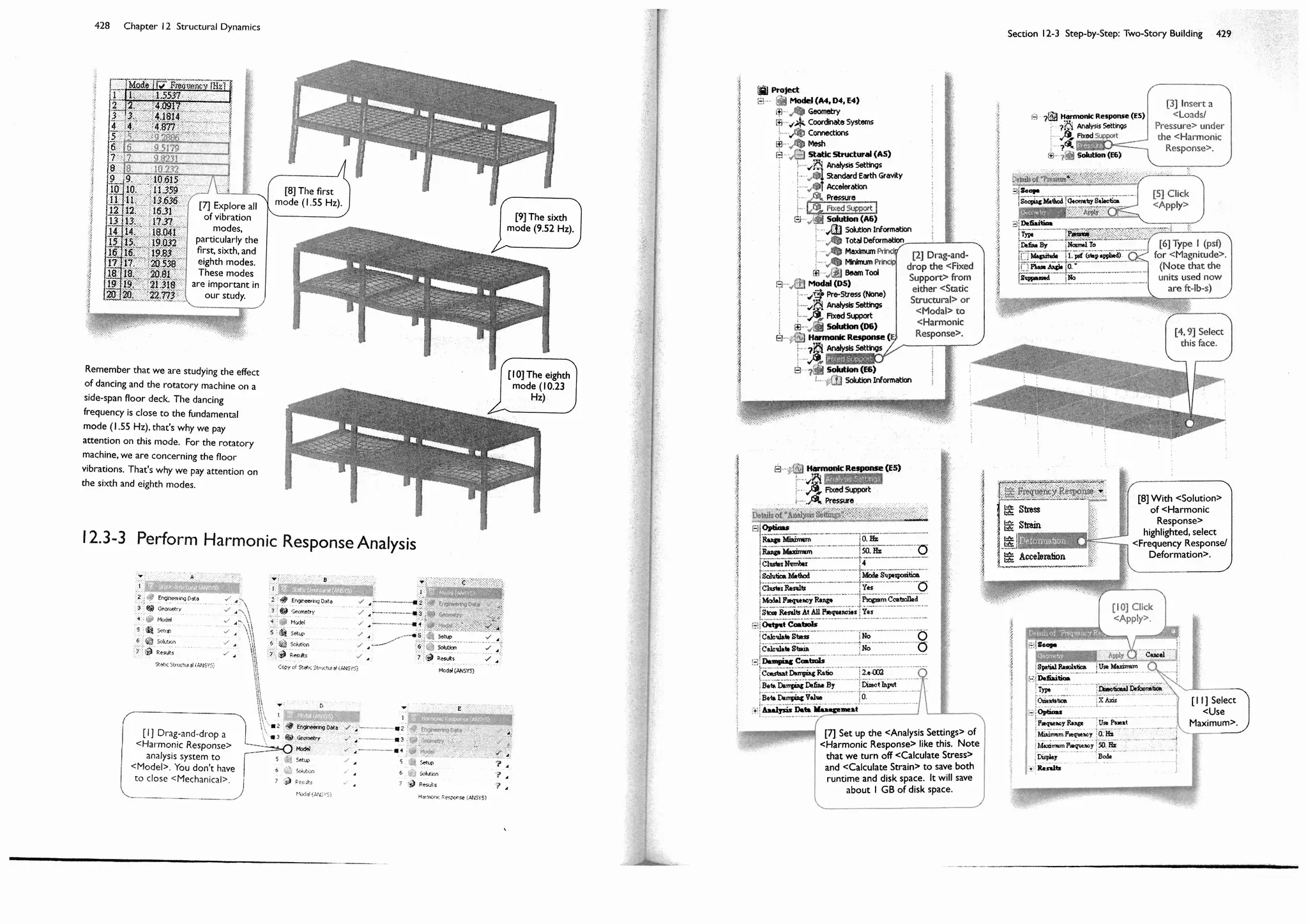
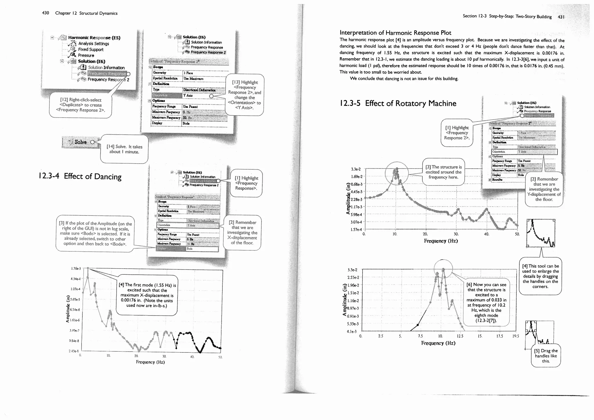
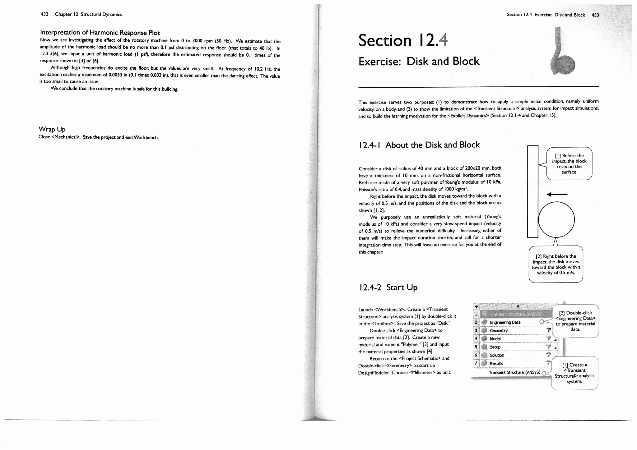
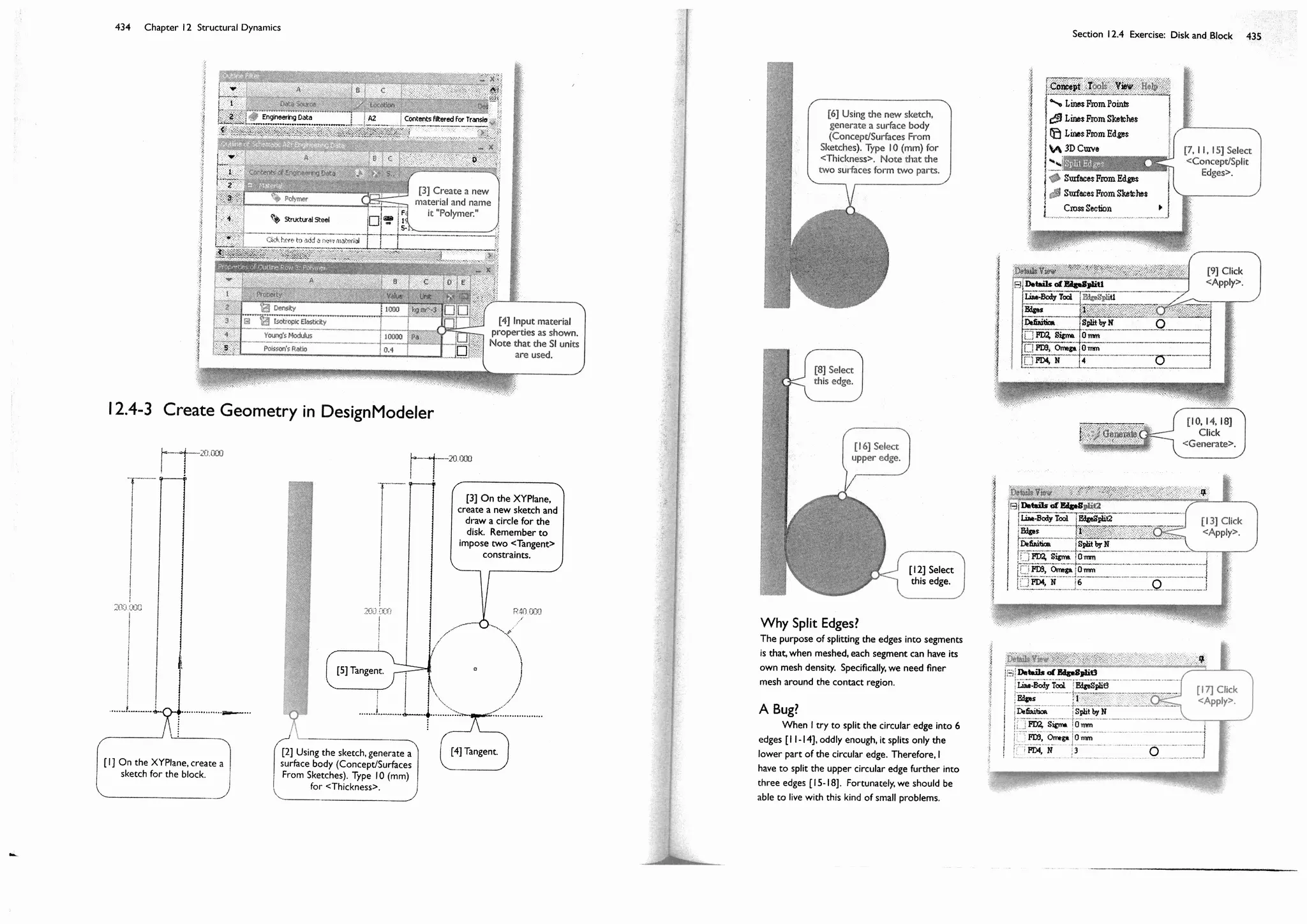
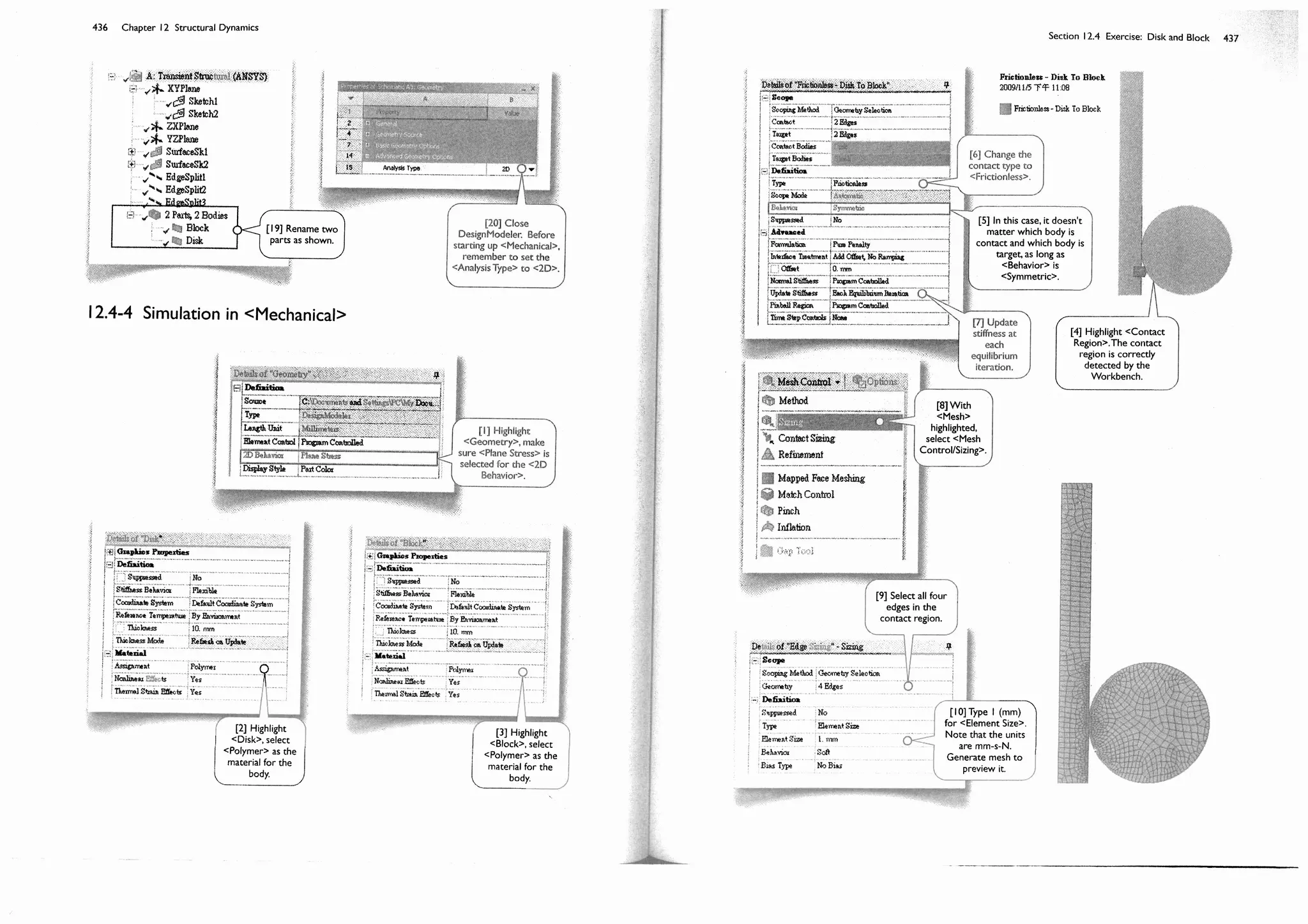
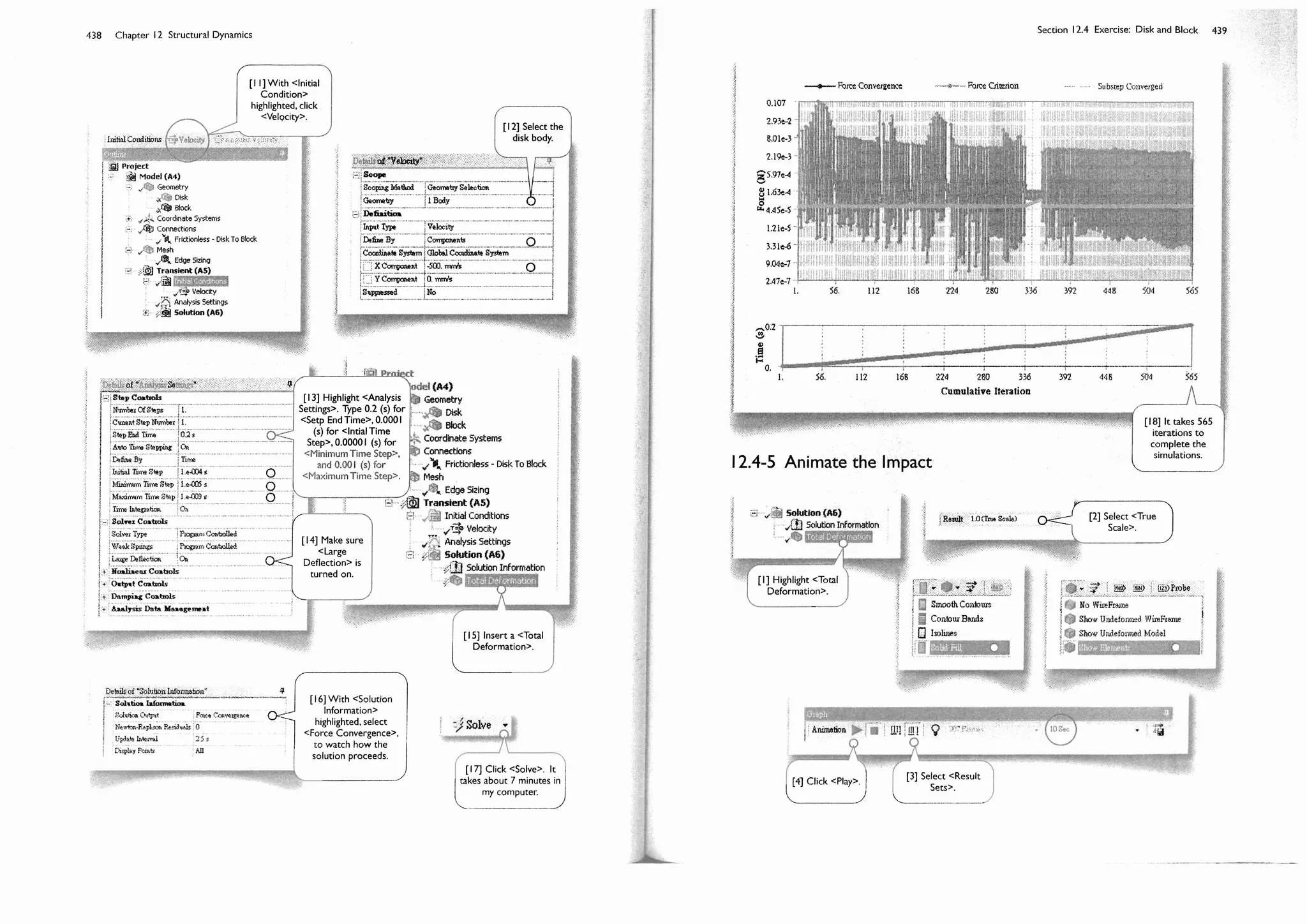
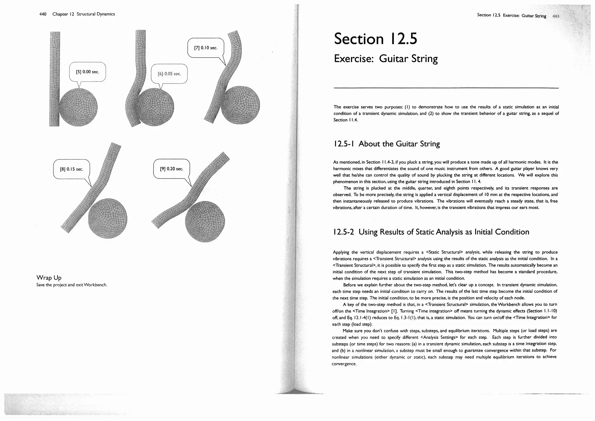
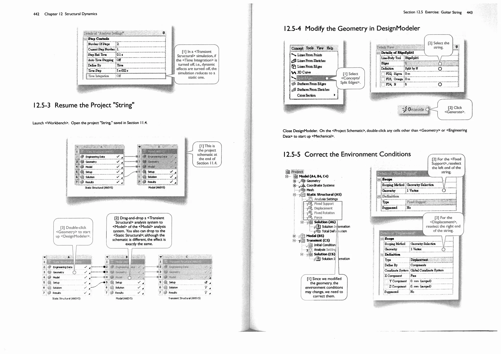
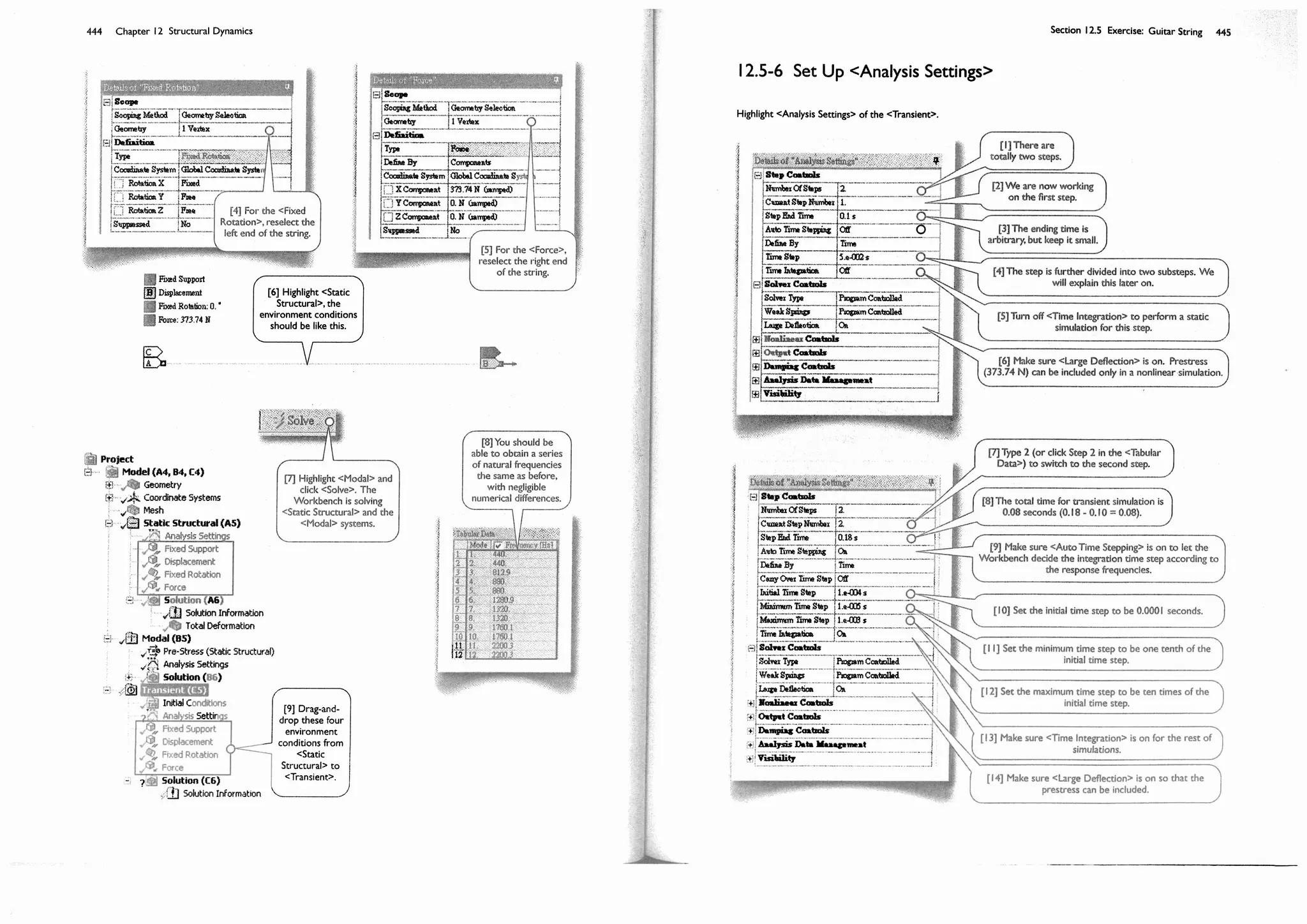
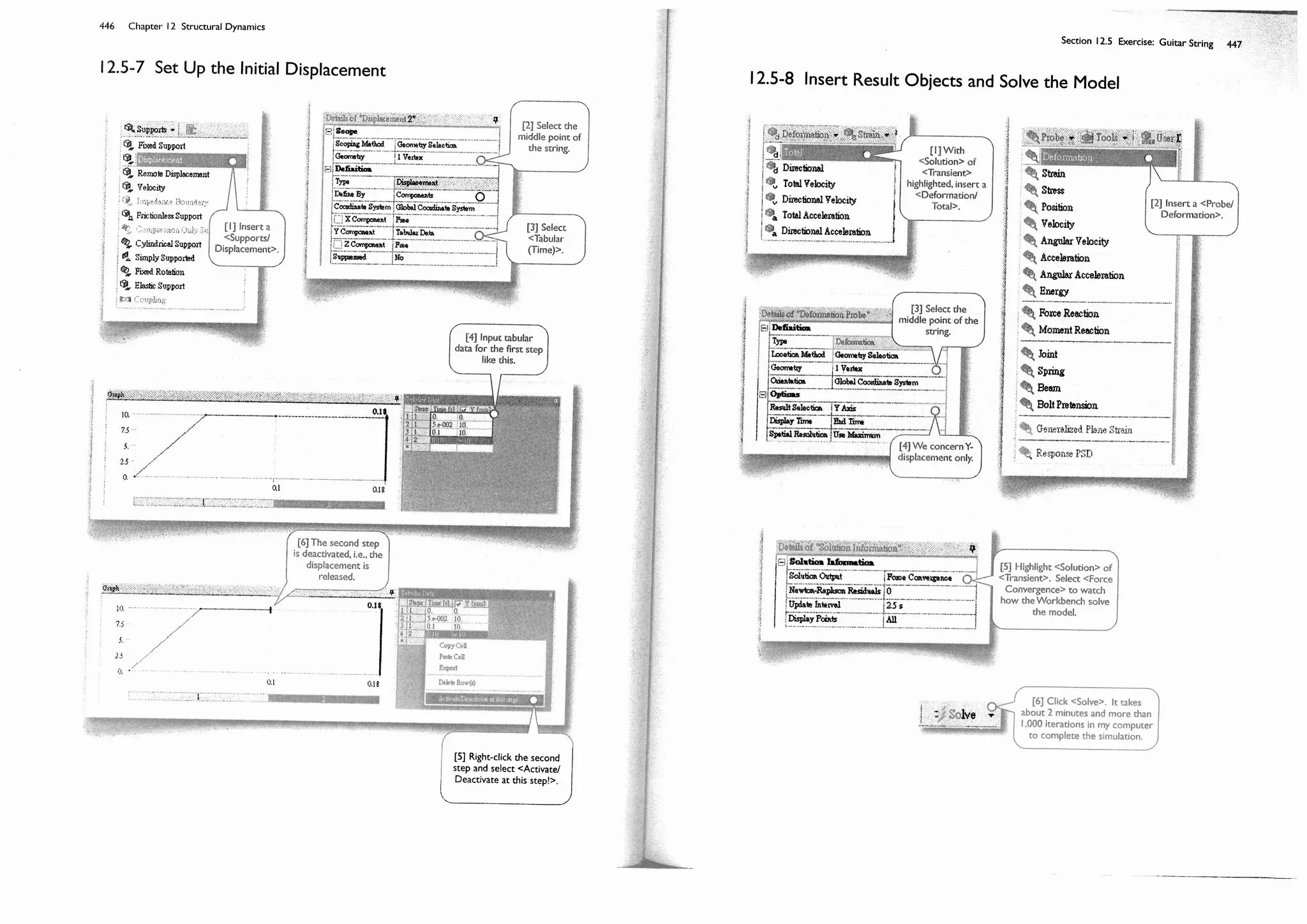
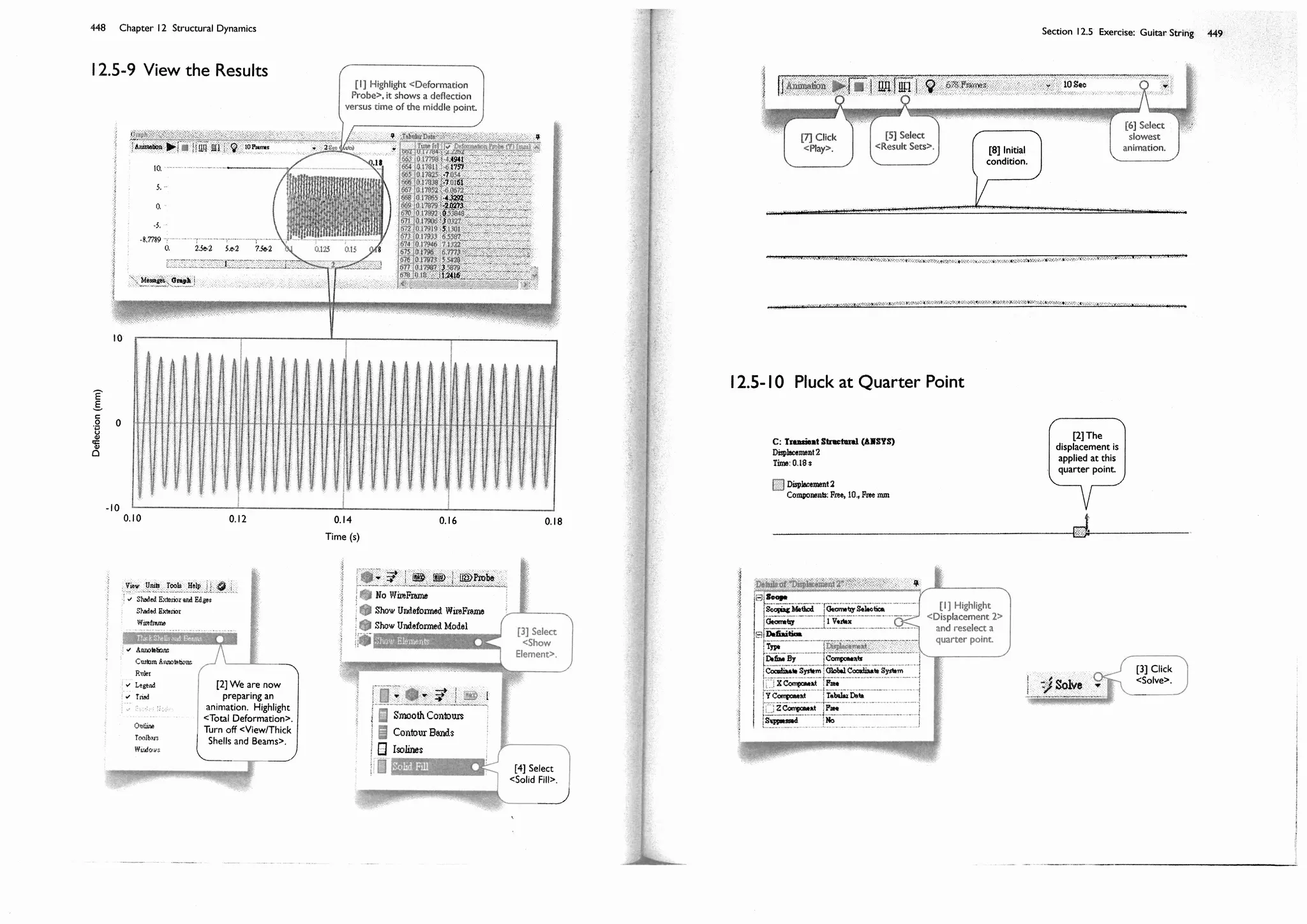
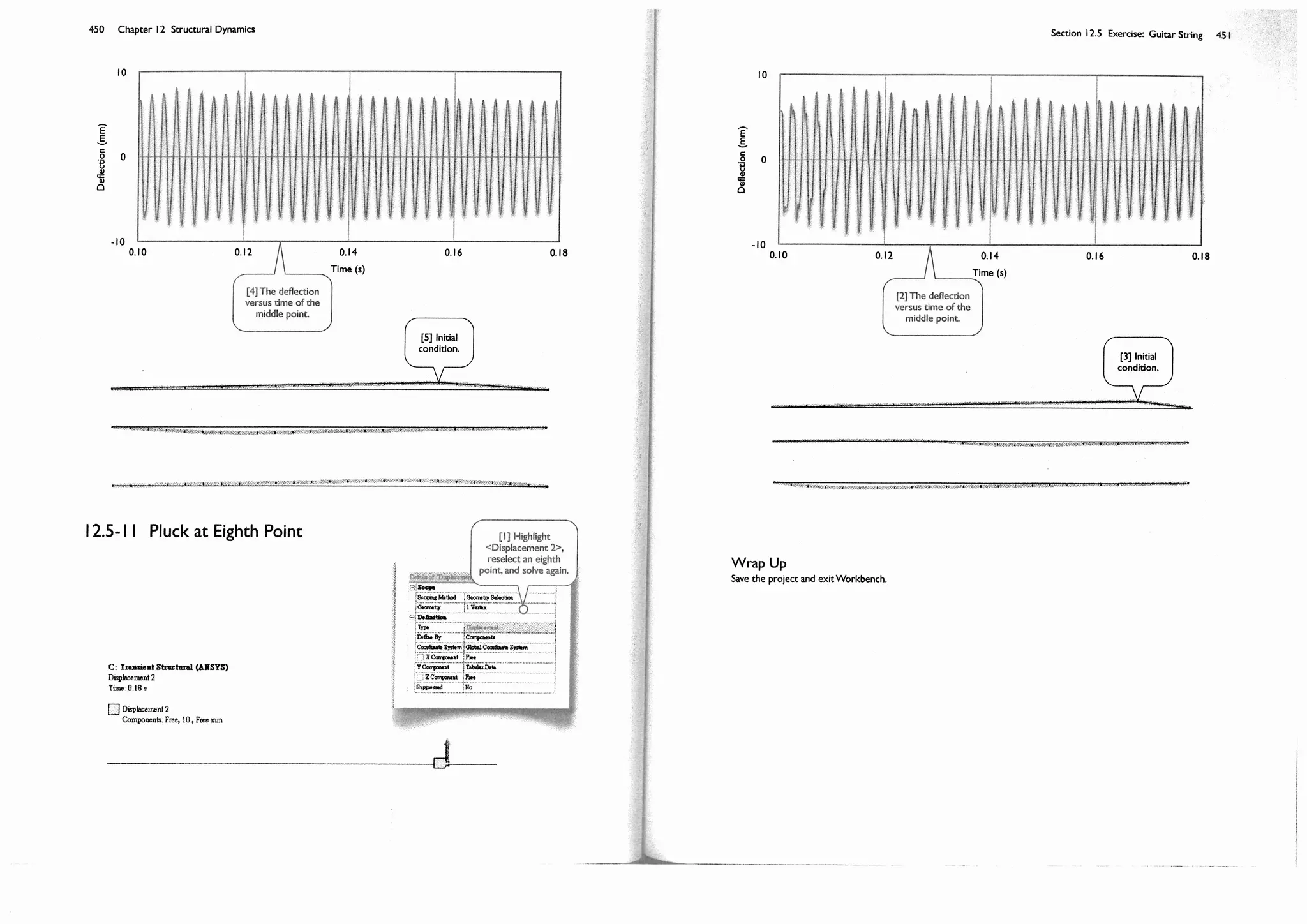
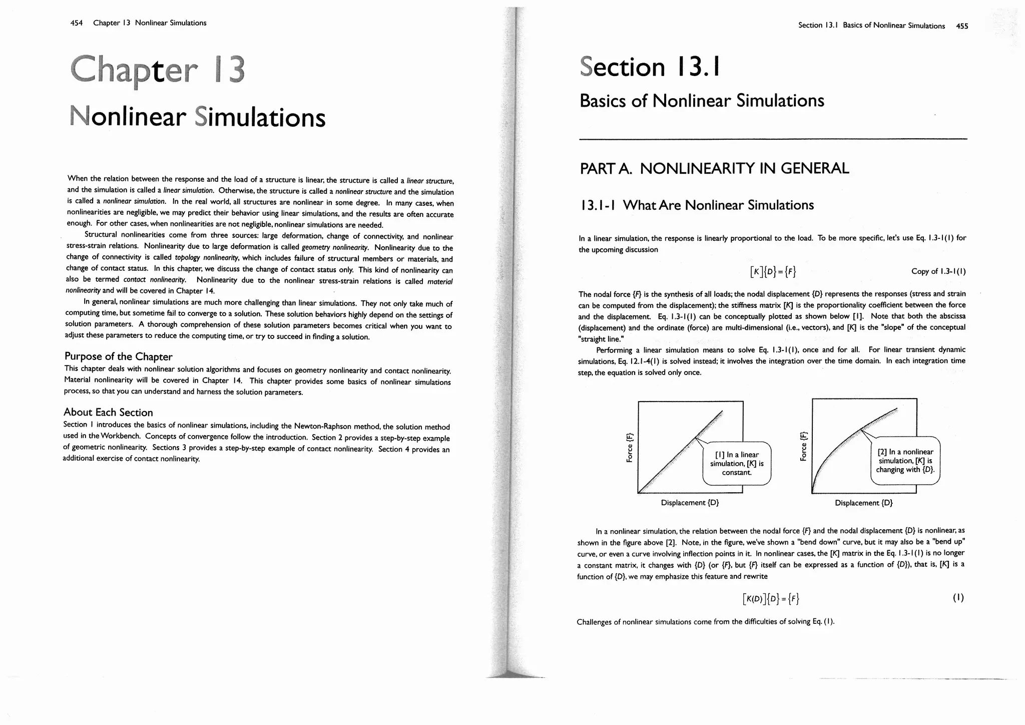
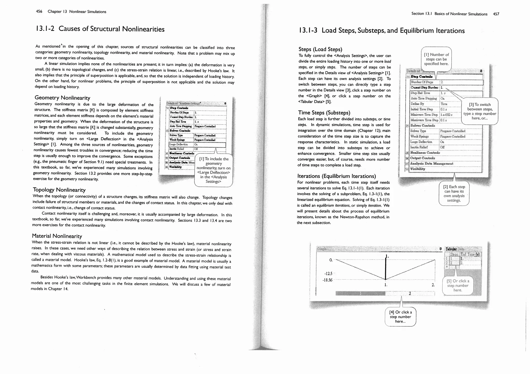
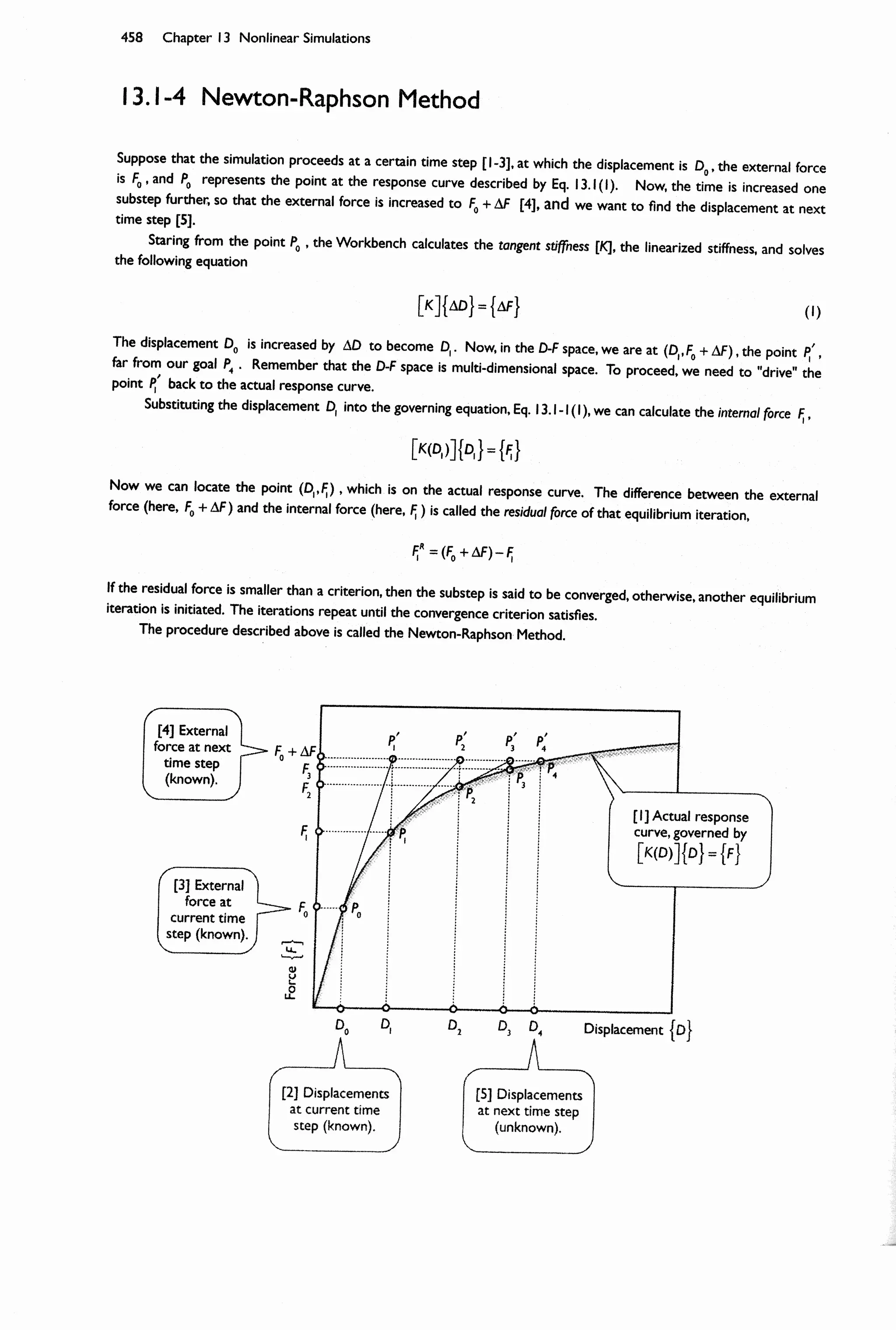
![Section 13.1 Basics of Nonlinear Simulations 459
13.1-5 Force Convergence and Displacement Convergence
In the last subsection, we stated that when the residual force FR
is smaller than a criterion, then the substep is said to
be converged. This statement is not strictly correct. There are at most four convergence criteria that can be activated
under your control, namely, force convergence [1], displacement convergence [2], moment convergence [3], and
rotation convergence [4]. The moment convergence and rotation convergence can be activated only when shell
elements or beam elements are used in the model. These convergence monitoring methods are all default to
<Program Controlled>, that is, the Workbench automatically turns on any of them when it is appropriate. You may
manually turn off or turn on any of them.
When you turn on any of them, you may specify a <Value>, a <Tolerance>, and a <Minimum Reference>. The
criterion is then
Criterion = maximum(Tolerance Value, Minimum Reference)
The force (or moment) convergence satisfies when
FR
< Criterion (1)
The displacement (or rotation) convergence satisfies when
D < Criterion (2)
Where denotes the norm of the underlying vector, and is called a convergence value. The <Value> defaults to
<ANSYS Calculated>, which usually means the current maximum value. For example, in the example of Section
13.1-4, the current maximum force value is F0
, and the current maximum displacement value is D0
. The
<Tolerance> defaults to 0.5%. Note that setting up a <Minimum Reference> is to avoid a never-convergent situation
when <Value> is near zero.
[1]You can turn
on <Force
Convergence> and
set the criterion.
[2]You can turn
on <Displacement
Convergence> and
set the criterion.
[3] When shell
elements or beam
elements are used,
<Moment
Convergence> can be
activated.
[4] When shell
elements or beam
elements are used,
<Rotation
Convergence> can be
activated.](https://image.slidesharecdn.com/huei-huanglee-finiteelementsimulationswithansysworkbench12-2010-151020015452-lva1-app6892/75/Finite-Element-Simulations-with-ANSYS-Workbench-2012-279-2048.jpg)
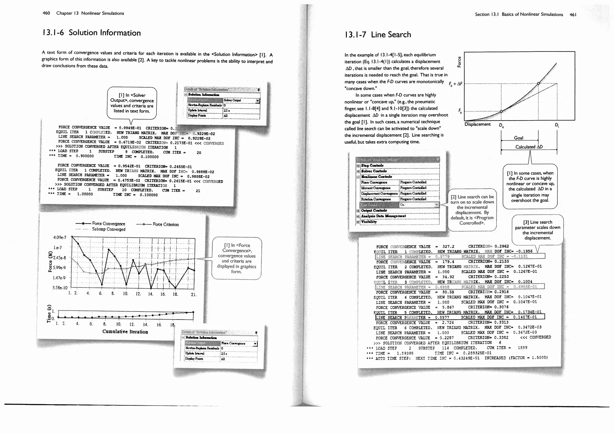
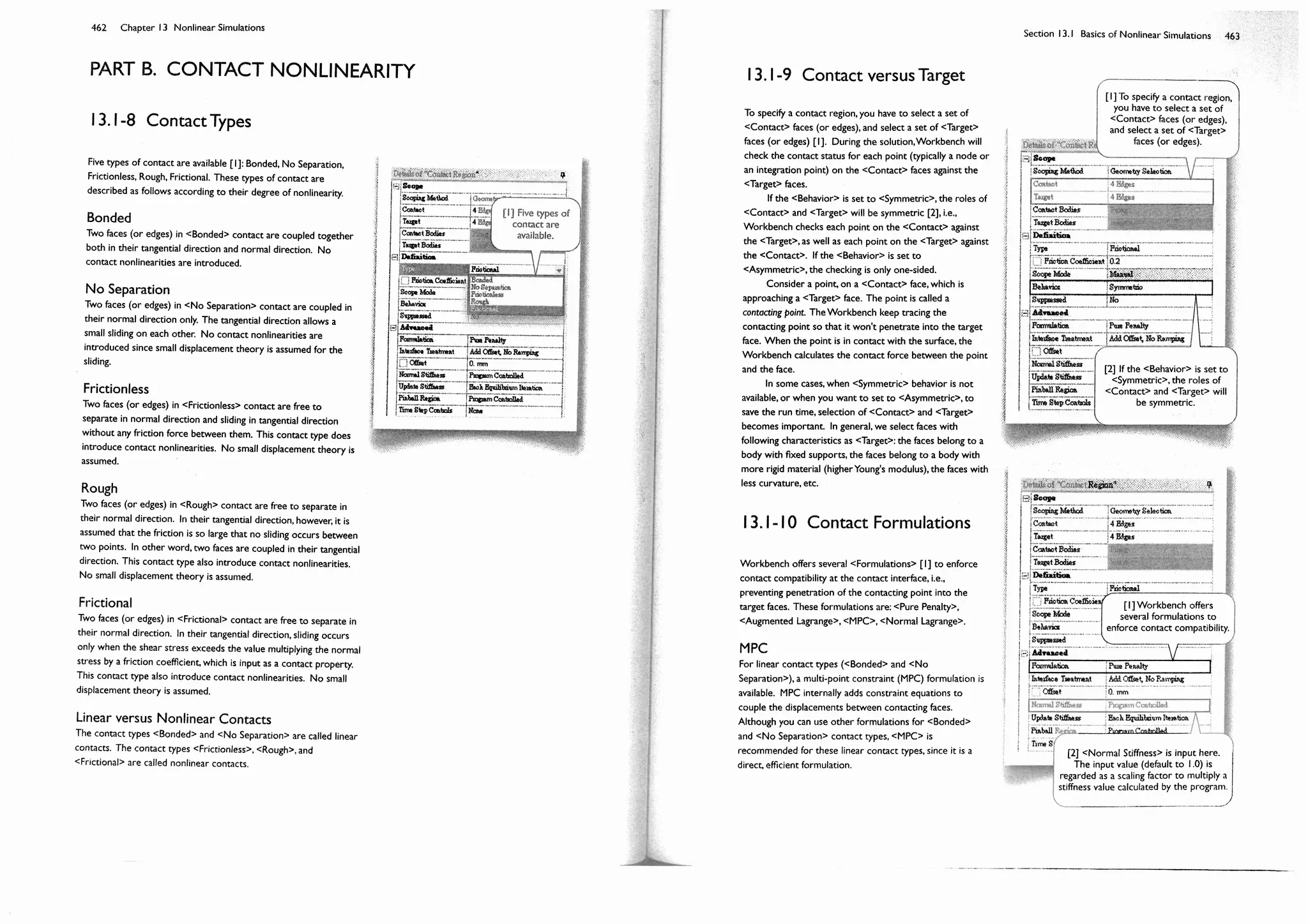
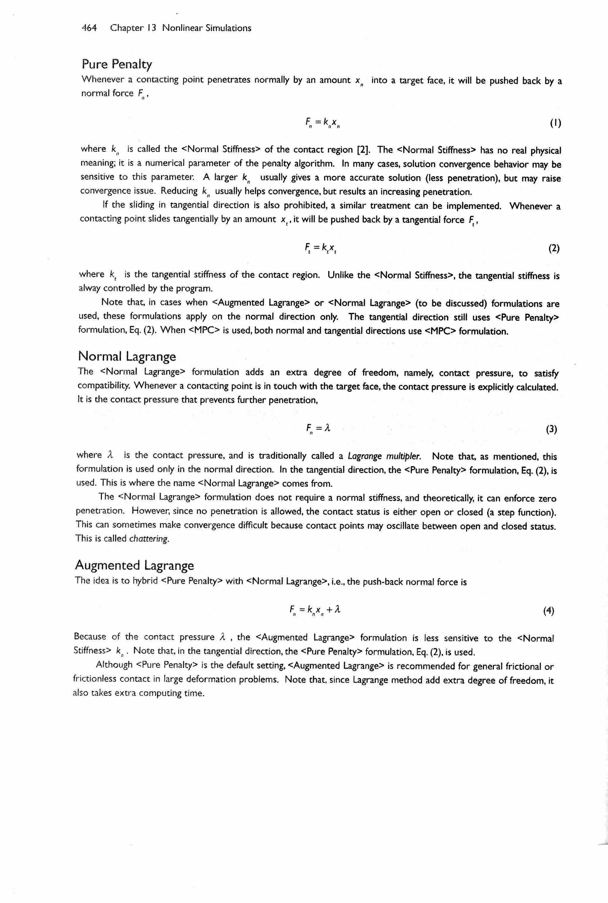
![Section 13.1 Basics of Nonlinear Simulations 465
13.1-11 Other Advanced Contact Settings
Pinball Region
The pinball is a sphere region, its radius can be defined in
<Pinball Region>. Consider again that a contacting point
approaches a target face. Using the contacting point as
the center of a pinball, for the nodes on the target face
that are within the pinball region, they are considered to
be in "near" contact and will be monitored. Nodes
outside of the pinball region will not be monitored.
If the <Bonded> type is specified, surfaces that have
gap smaller than the pinball radius is treated as bonded.
Interface Treatment
For <Bonded> contact type, a large enough pinball radius
may allow any gap between contacting faces to be ignore.
For <Frictional> or <Frictionless> contact types, an
initial gap is not automatically ignored, no matter how
large the pinball is used, since the gap may represents the
geometry.
If an initial gap is present [1] and a force is applied,
one part may "fly away" relative to another part [2] if the
initial contact is not established right at the end of the
time step.
To alleviate situations where a gap (clearance) is
modeled but needs to be ignored to establish initial
contact for <Frictional> or <Frictionless> contact types,
the <Interface Treatment> can internally offset the
contact surfaces by a specified amount. Note that this
treatment is intended for small gaps. Don't apply it in a
large gap.
Time Step Controls
<Time Step Controls> tries to enhance convergence by
allowing adjustments of time step size based on changes
in contact behavior.
By default, contact behavior does not affect auto
time stepping, since adjustment of time step based on
contact behavior may increase computing time too much.
When turning on <Time Step Controls>,
Workbench will adjust the time step size based on
contact behavior.
Update Stiffness
By default, structural stiffness is not updated upon the
change of contact behavior, to save the computing time.
Turning on <Update Stiffness> enhance convergence,
with the cost of computing time.
Force
[1] An
initial gap is
present.
[2] This part may
"fly away" relative
to another part.](https://image.slidesharecdn.com/huei-huanglee-finiteelementsimulationswithansysworkbench12-2010-151020015452-lva1-app6892/75/Finite-Element-Simulations-with-ANSYS-Workbench-2012-283-2048.jpg)
![466 Chapter 13 Nonlinear Simulations
60
20
20
40
Section 13.2
Step-by-Step: Translational Joint1
A translational joint is used to connect two machine components, so that the relative motion of two components is
restricted to translate in a specific direction. Conventionally, translational joints are designed as mechanisms,
composed by parts, between which the clearance or interference are inevitable; they either decrease precision or
increase friction. The translational joint discussed in this section is not a mechanism; it is a unitary flexible structure, in
which no clearance or interference exist.
The translational joint [1-4] is made of POM (polyoxymethylene, a plastic polymer), which has a Young's modulus
of 2 GPa and a Poisson's ratio of 0.35. The most important design consideration is that the rigidity of translational
direction should be much less than all other directions, so that the motion can be restricted in that direction only.
Here, we want to explore the geometric nonlinearity of the structure: how the applied force increases
nonlinearly with the translational displacement. For this purpose, we will model the structure using line bodies
entirely. The goal of the simulation is to plot a force-versus-displacement chart. The unit system used in the simulation
is mm-s-N.
13.2-1 About the Translational Joint
[3] All connectors
have a cross section
of 10x10 mm.
[1] The
translational joint
is used to connect
two machine
components, so
that the relative
motion of the
components is
restricted in this
direction.
[4] A prototype of
translational joint. Note
that this prototype has no
horizontal "wings" on it.
[2] All leaf springs
have a cross
section of 1x10
mm.](https://image.slidesharecdn.com/huei-huanglee-finiteelementsimulationswithansysworkbench12-2010-151020015452-lva1-app6892/75/Finite-Element-Simulations-with-ANSYS-Workbench-2012-284-2048.jpg)
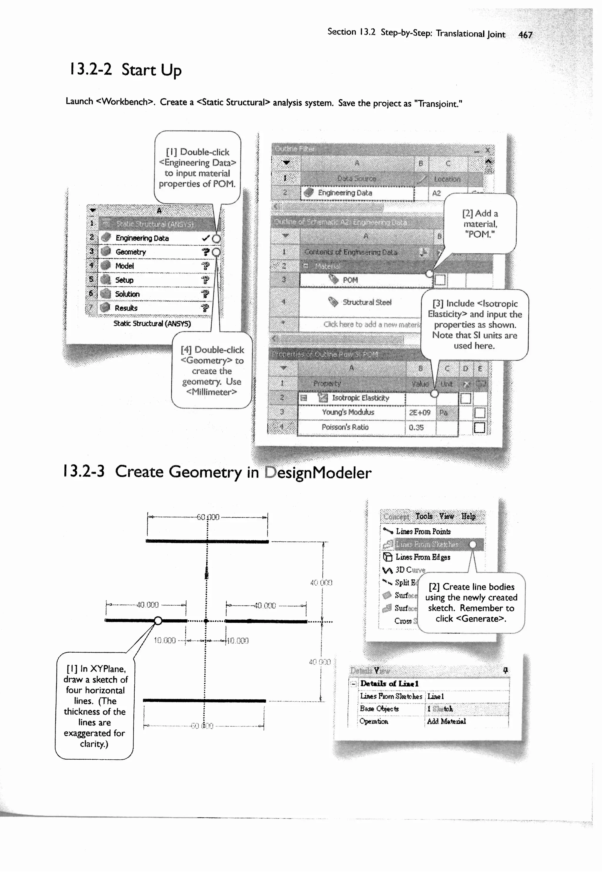
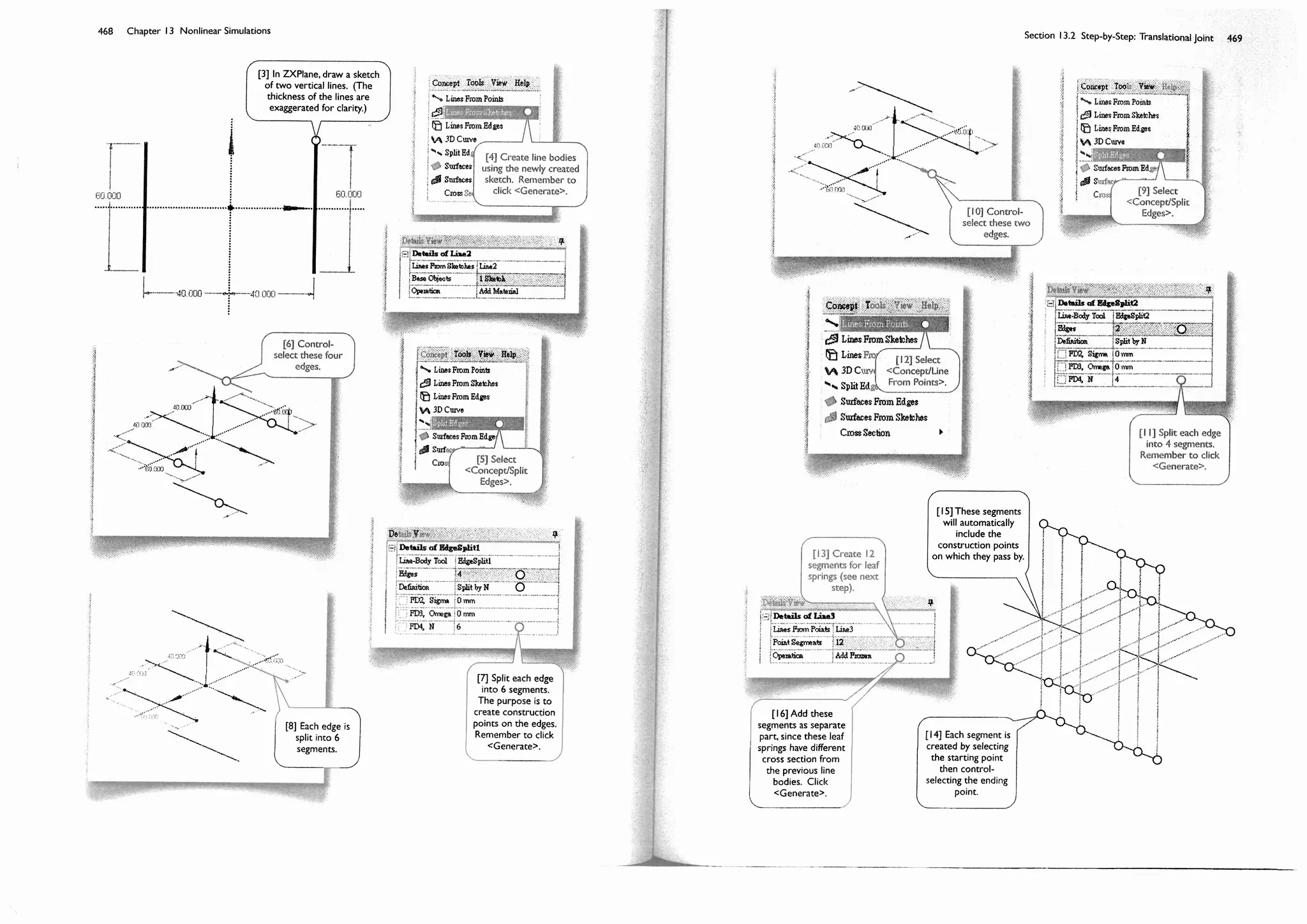
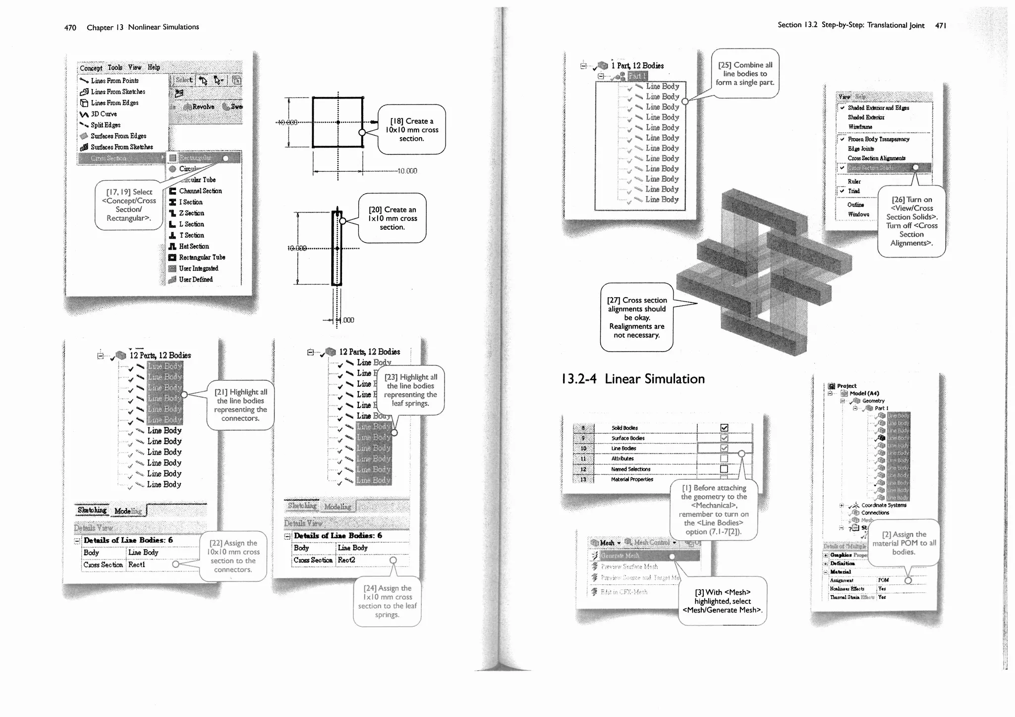
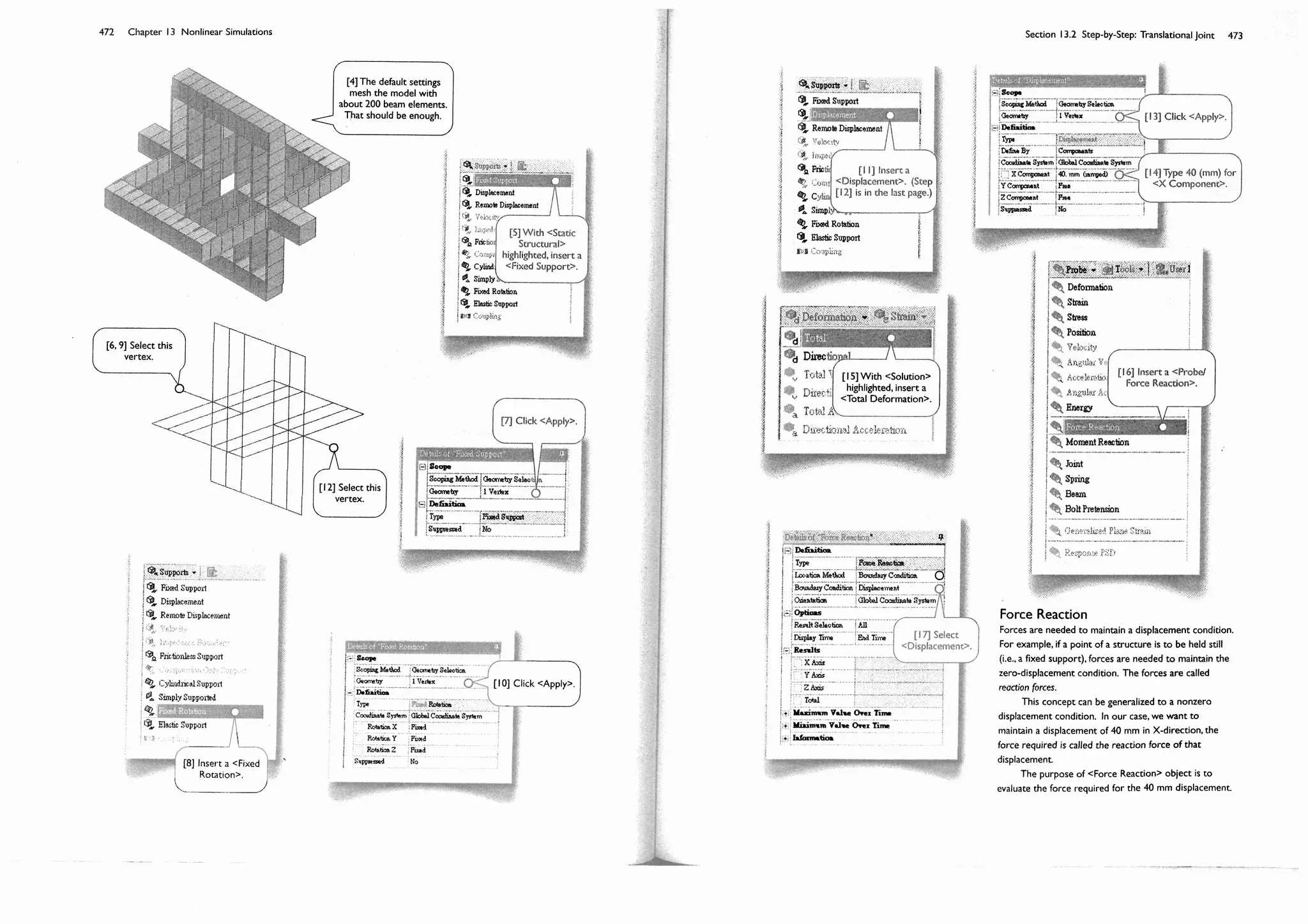
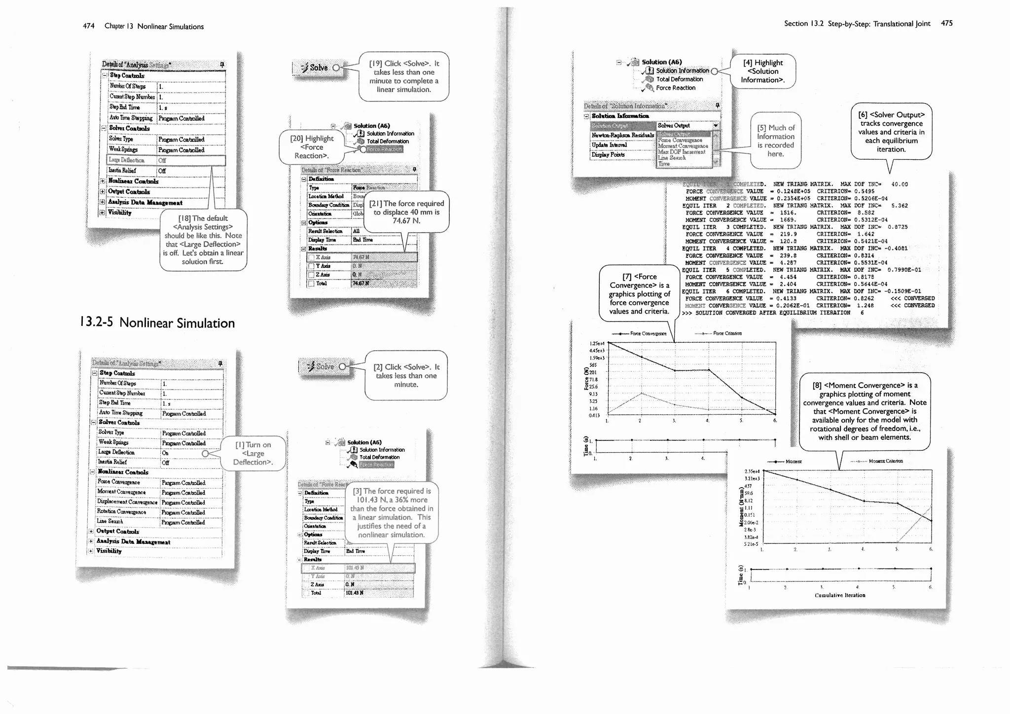
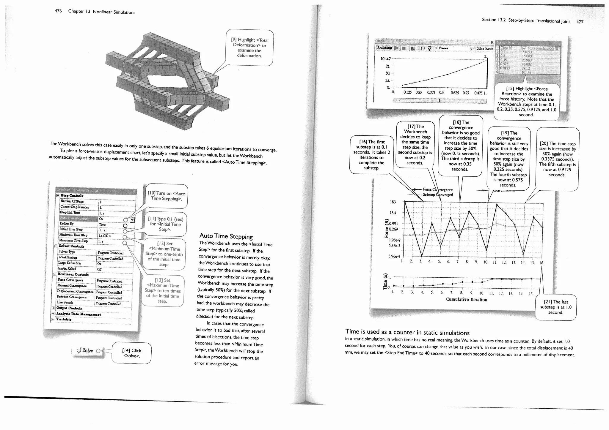
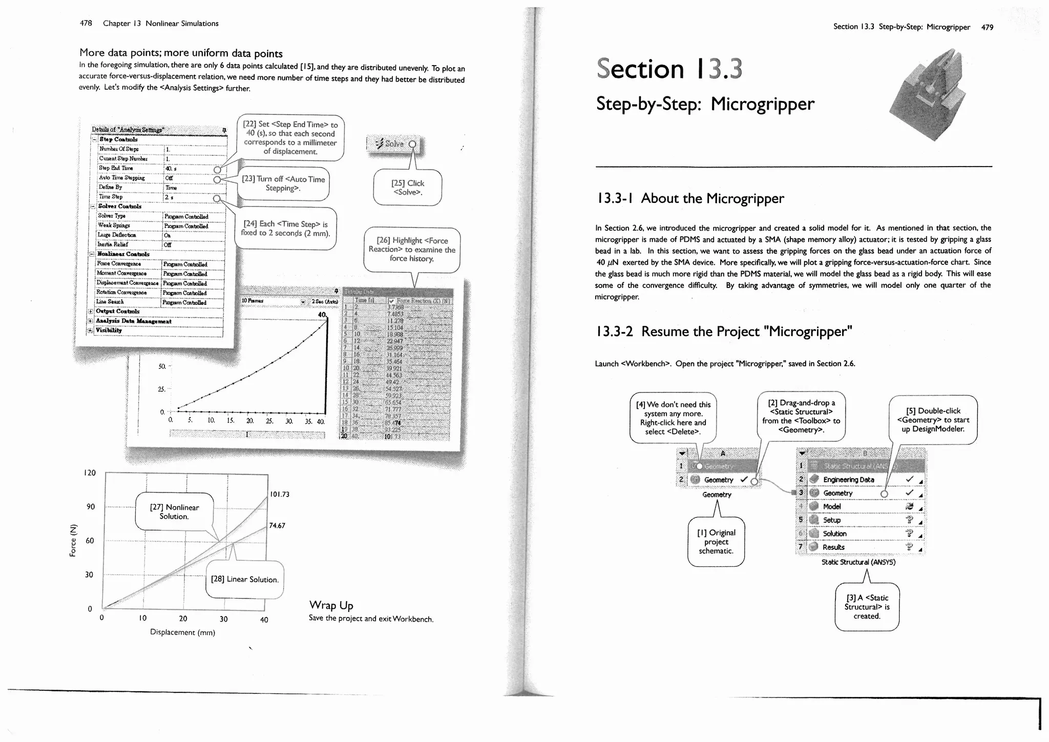
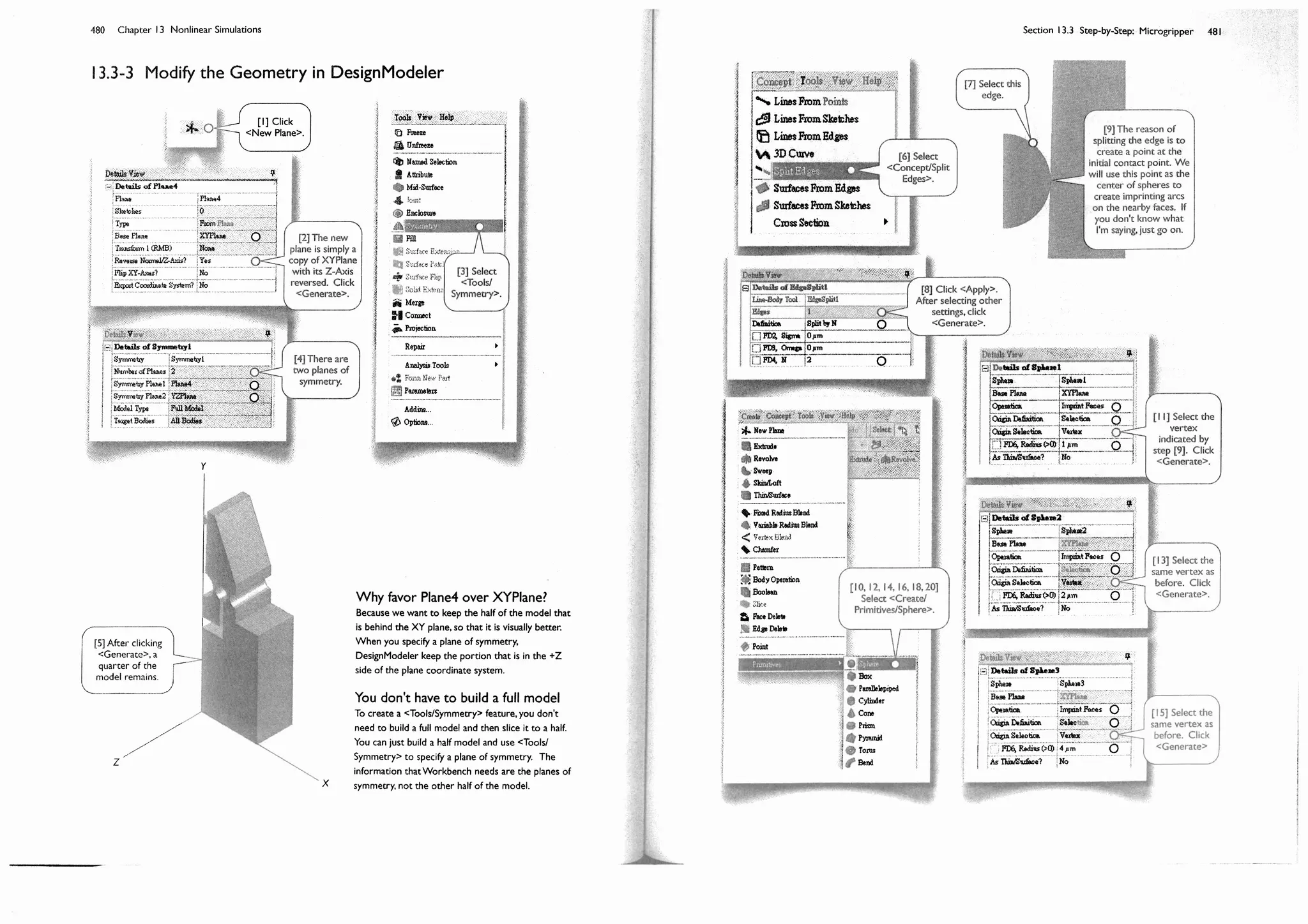
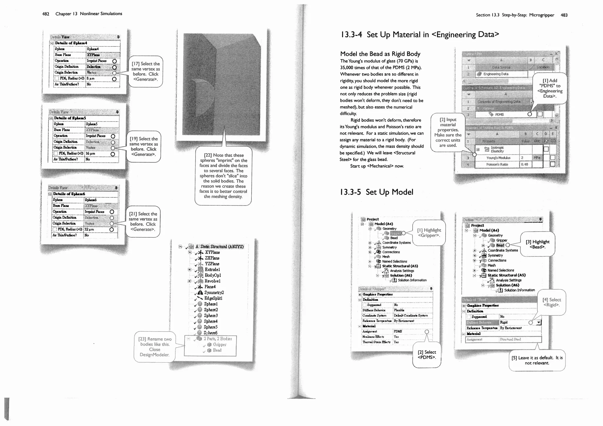
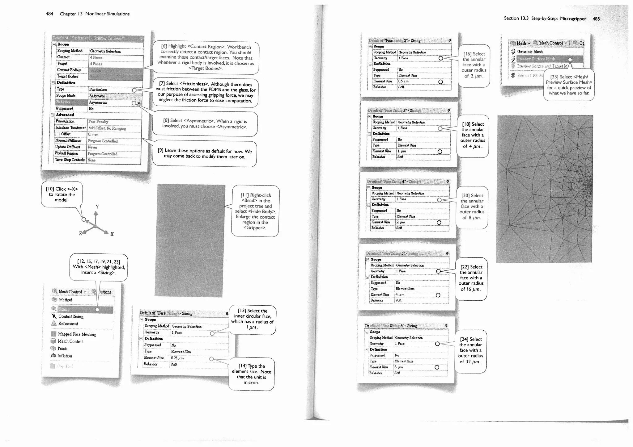
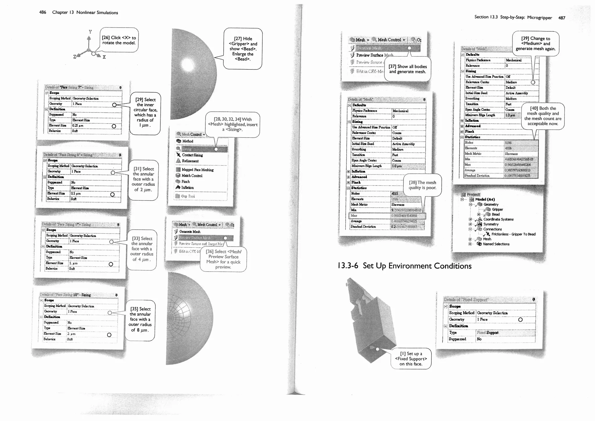
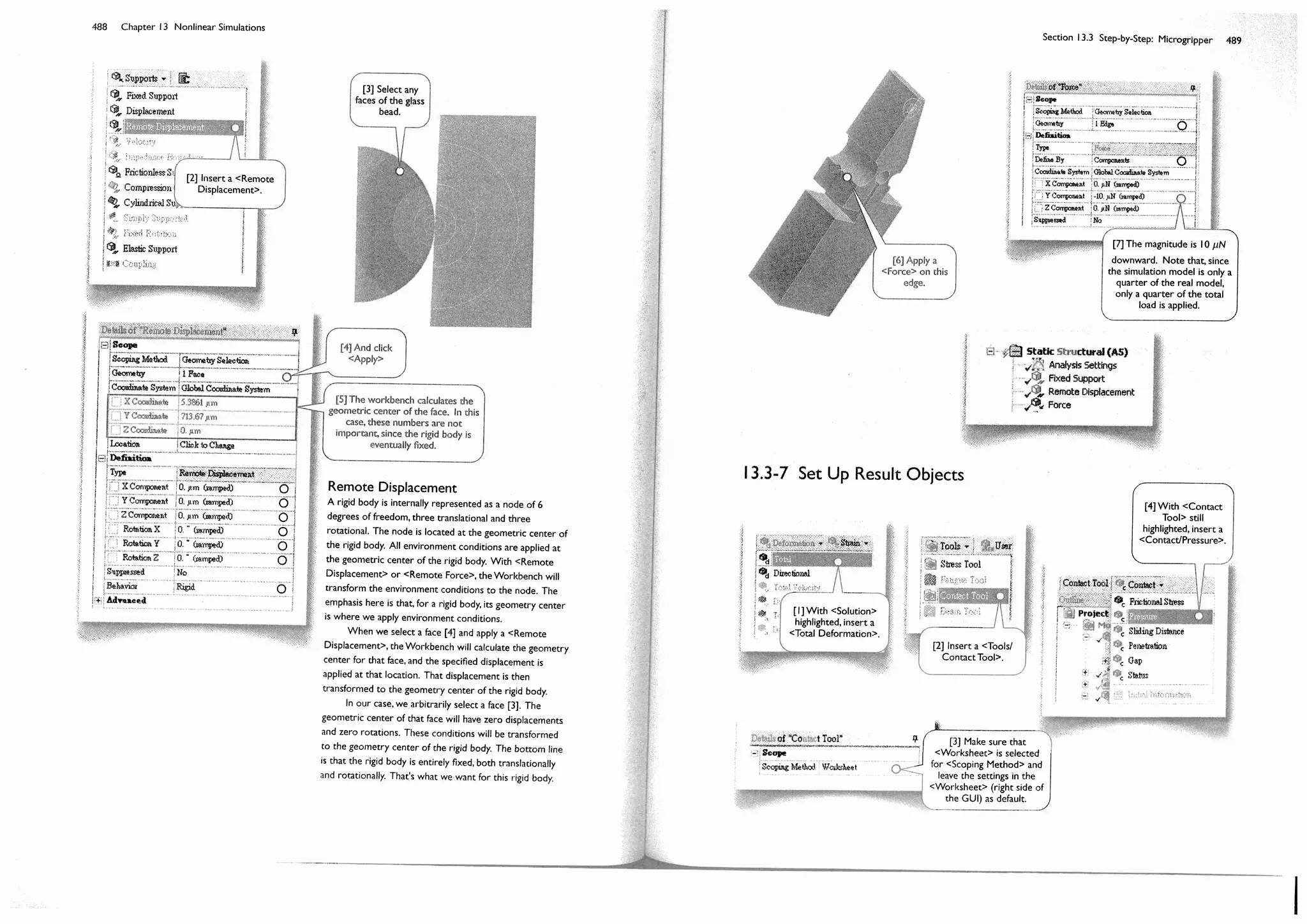
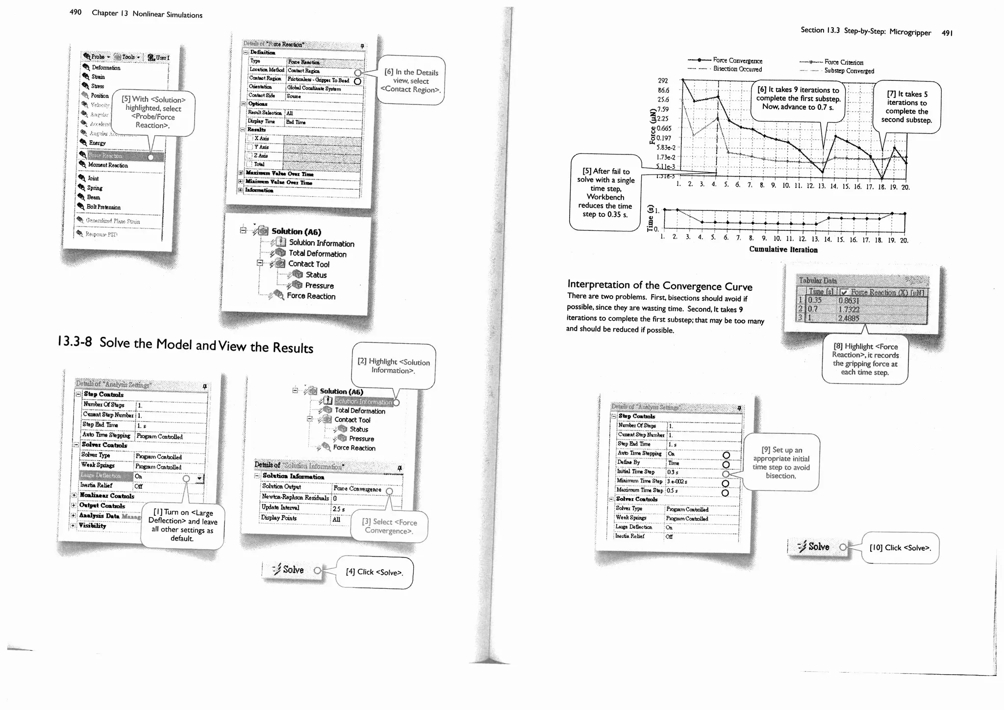
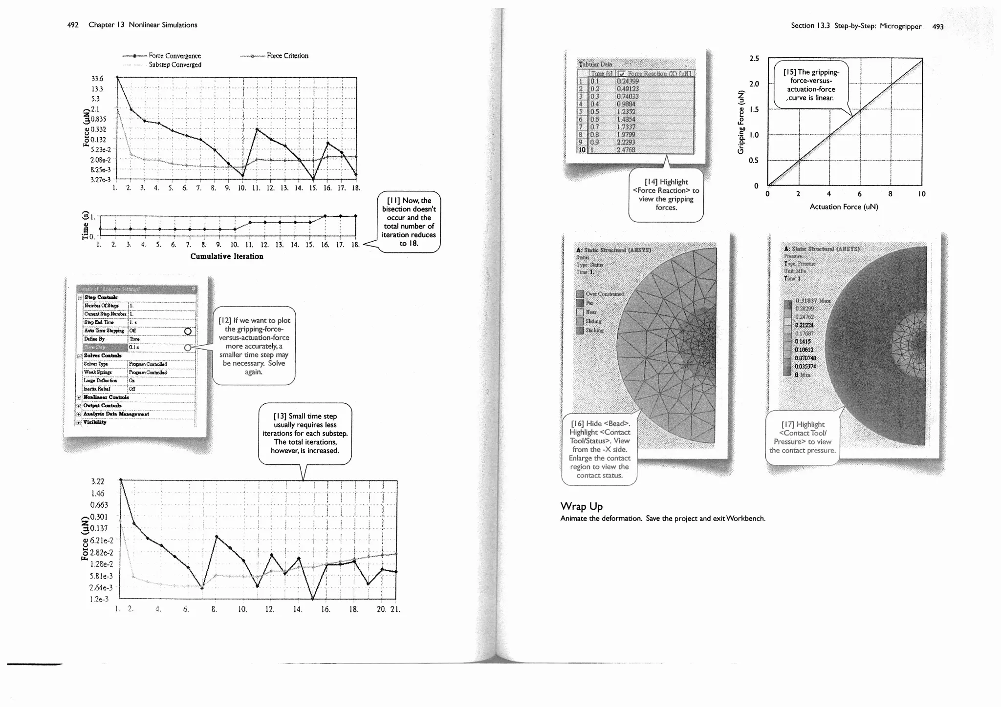
![494 Chapter 13 Nonlinear Simulations
Section 13.4
Exercise: Snap Lock
The snap lock consists of two parts: the insert [1] and the prongs [2]; it is fastened when pushed into position [3]. The
snap lock has a thickness of 5 mm and is made of a plastic material with a Young's modulus of 2.8 GPa and a Poisson's
ratio of 0.35. The coefficient of friction between the materials is 0.2. The purpose of the simulation is to find out the
force required to push the insert into the position and the force required to pull it out.
We will model the problem as a plane stress problem. Due to the symmetry, only one half of the model is used
in the simulation.
13.4-1 About the Snap Lock
7
20
20
7
10
30
17
7
5
10
5
8
Unit: mm.
All fillets has radius of 2 mm.
[3] After
snapping in.
[1] The insert.
[2] The prongs.](https://image.slidesharecdn.com/huei-huanglee-finiteelementsimulationswithansysworkbench12-2010-151020015452-lva1-app6892/75/Finite-Element-Simulations-with-ANSYS-Workbench-2012-299-2048.jpg)
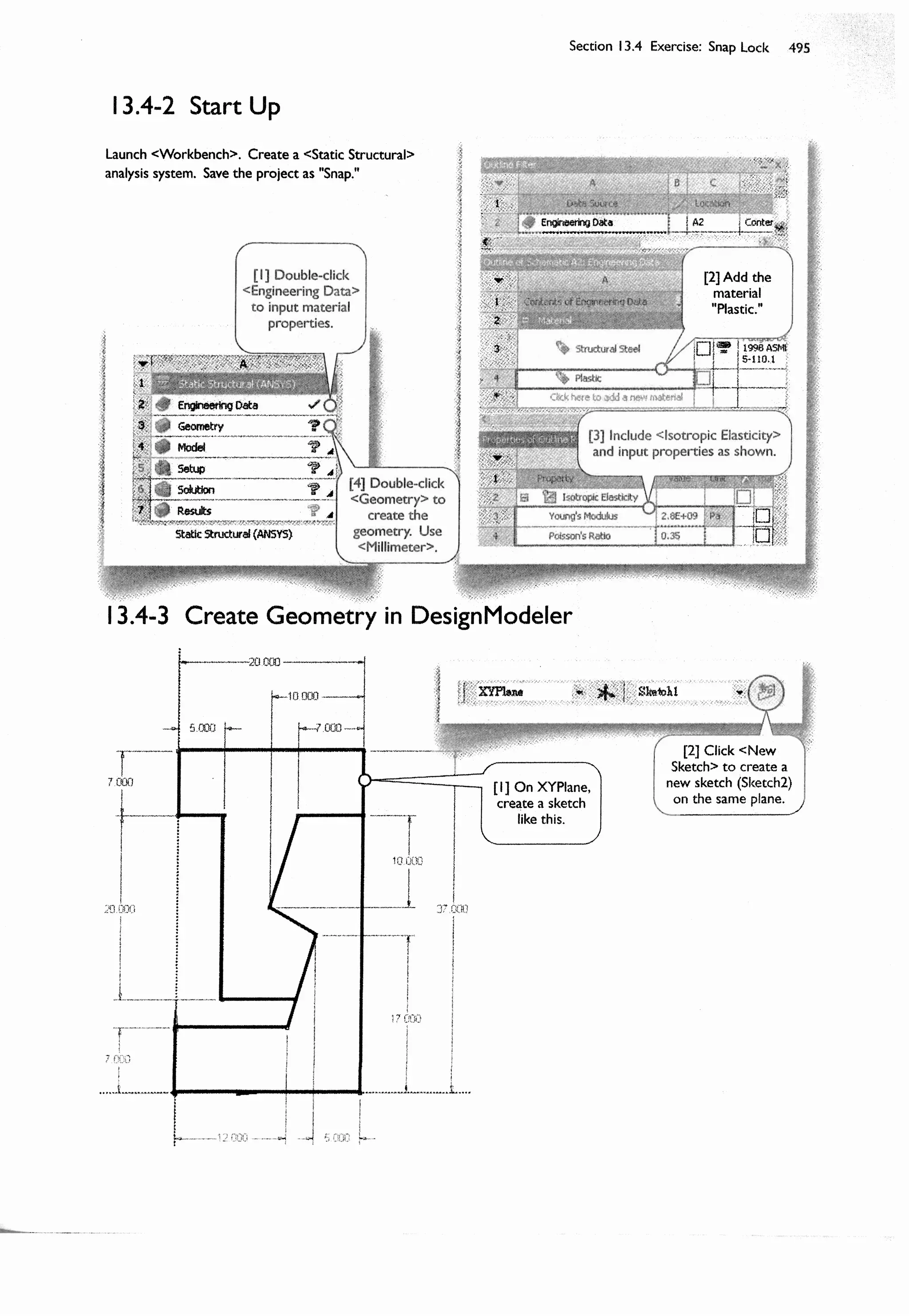
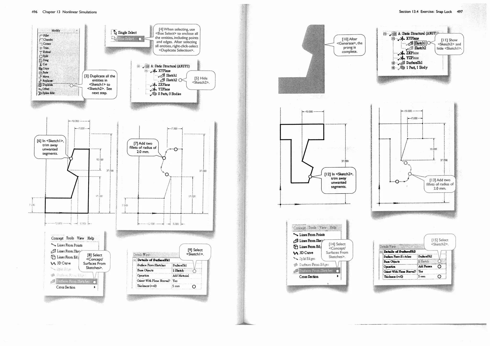
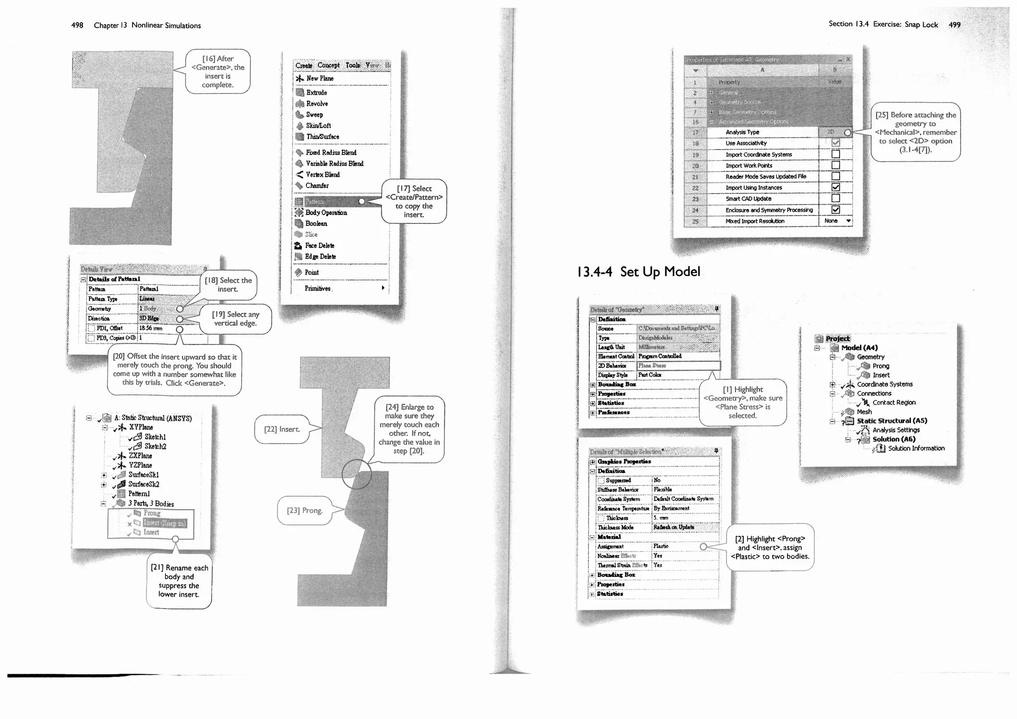
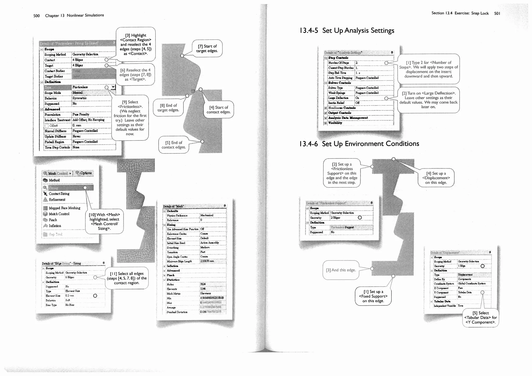
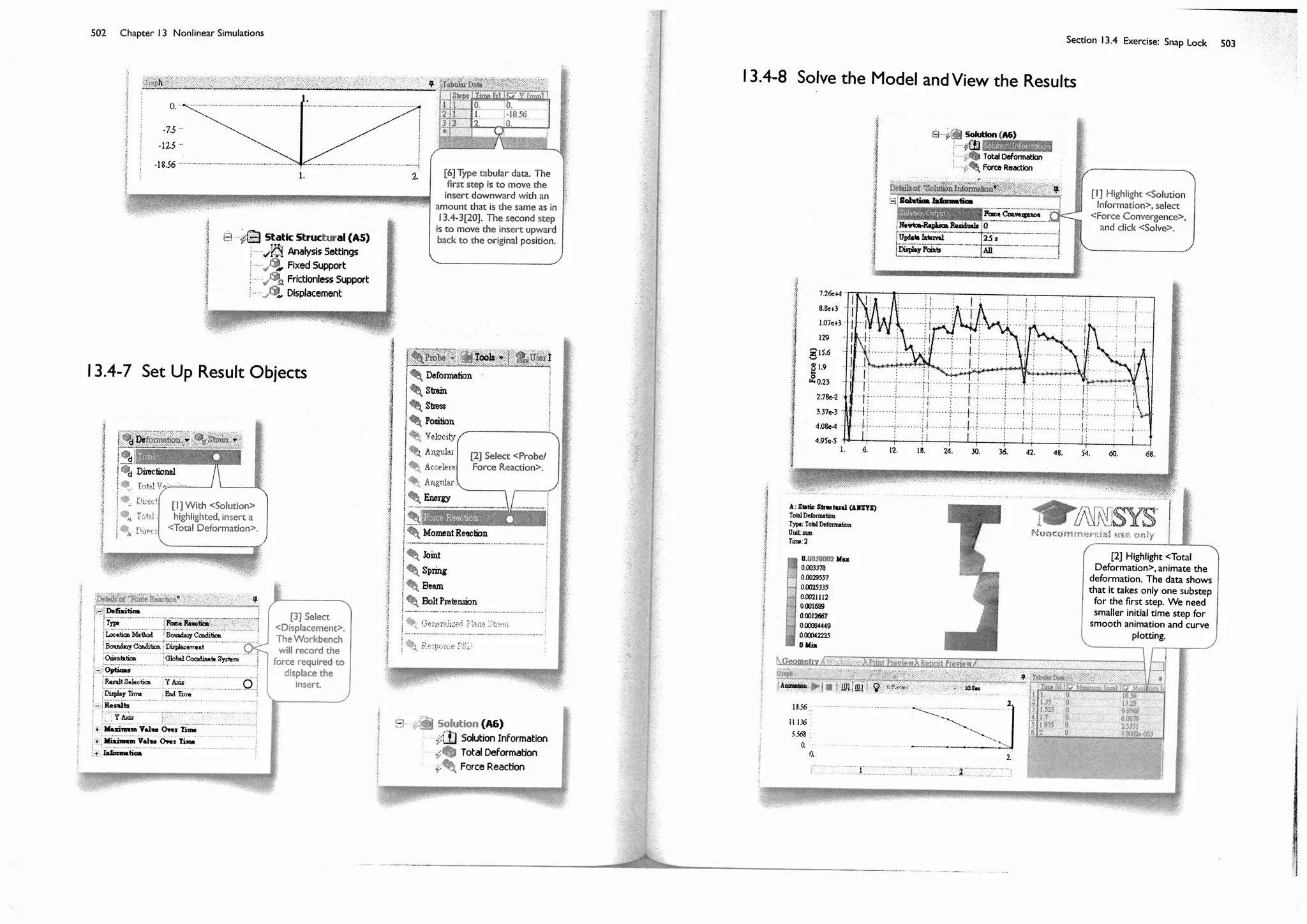
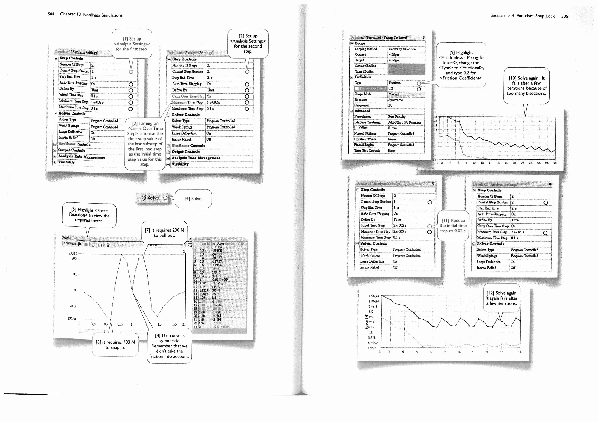
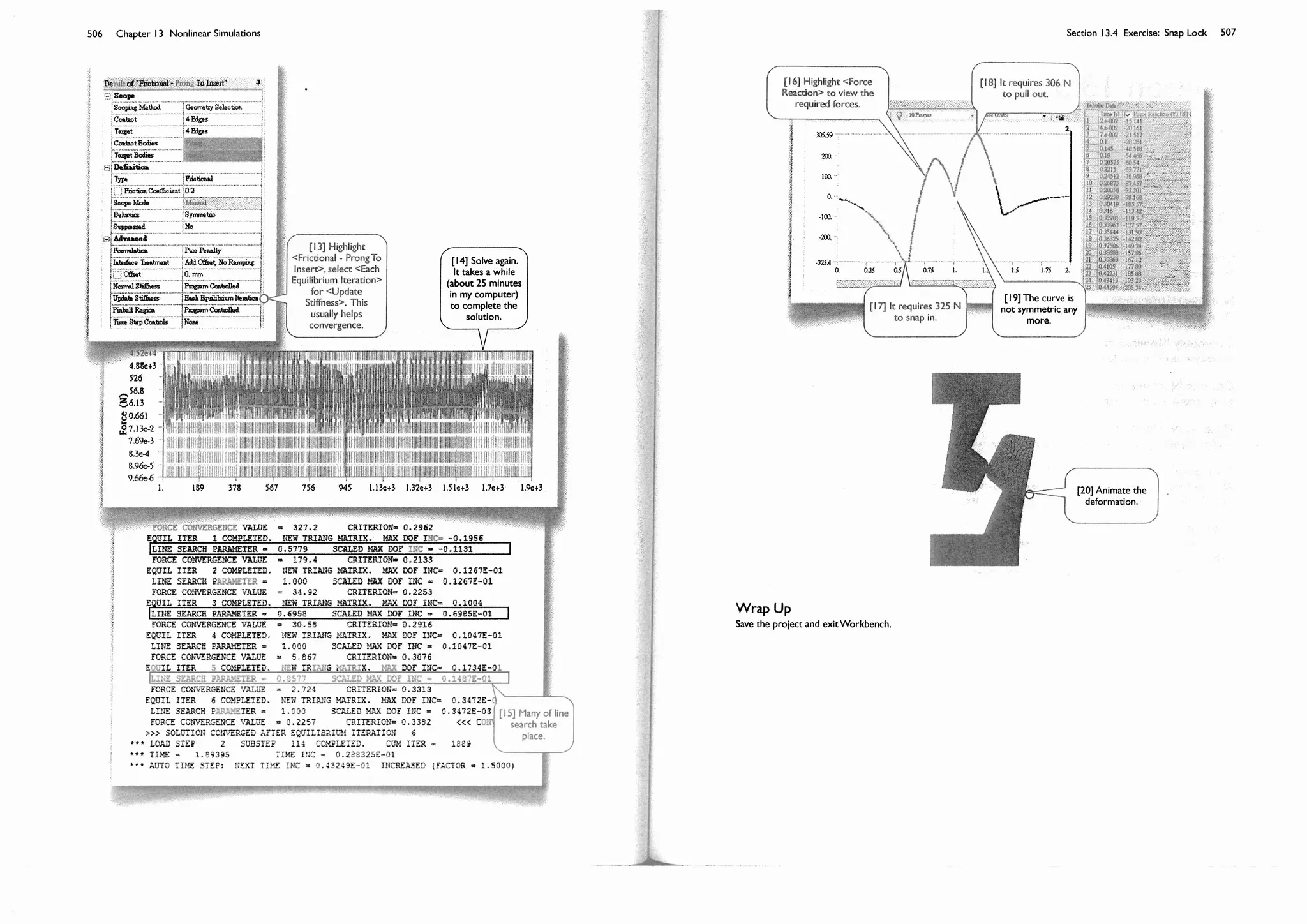
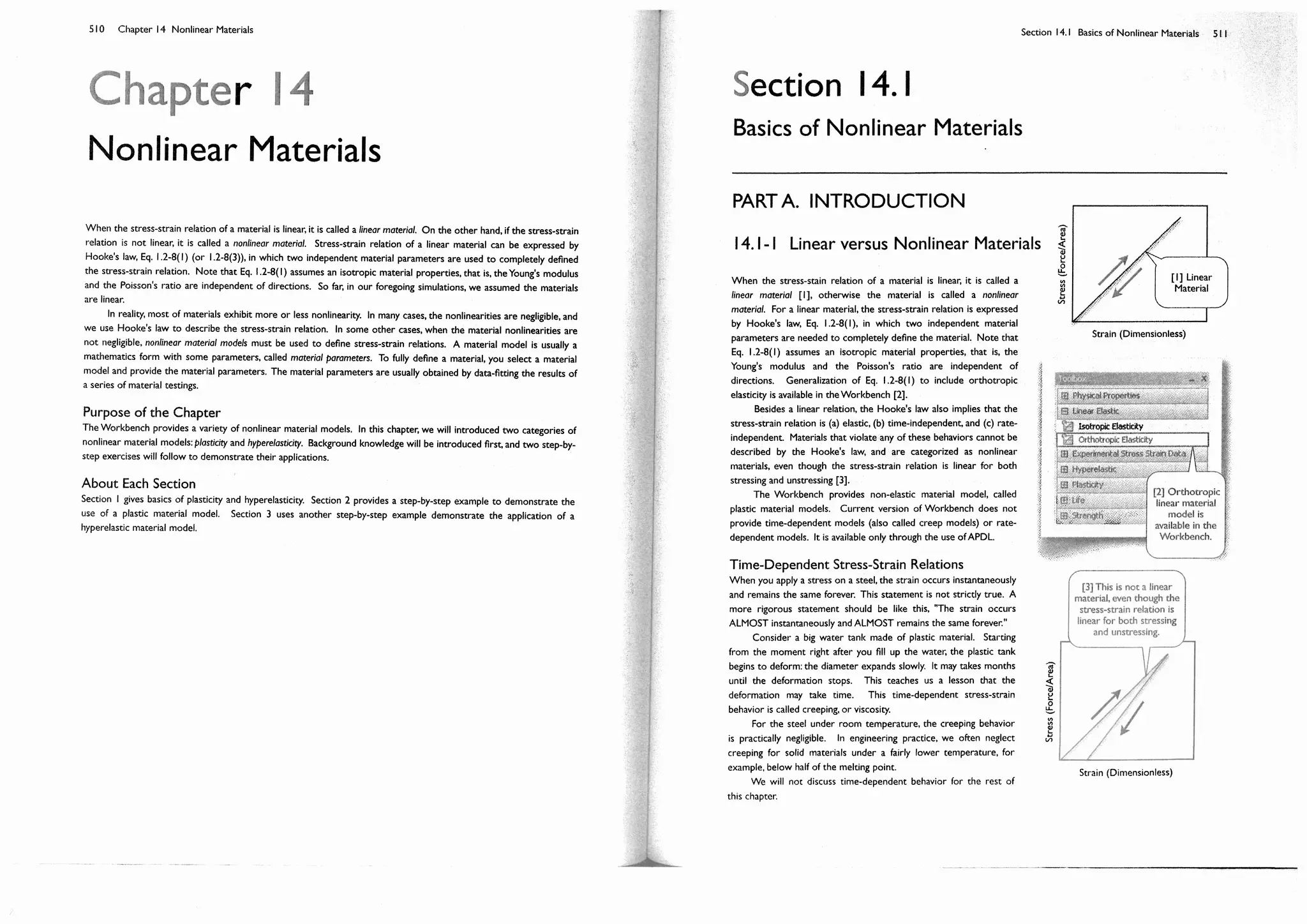
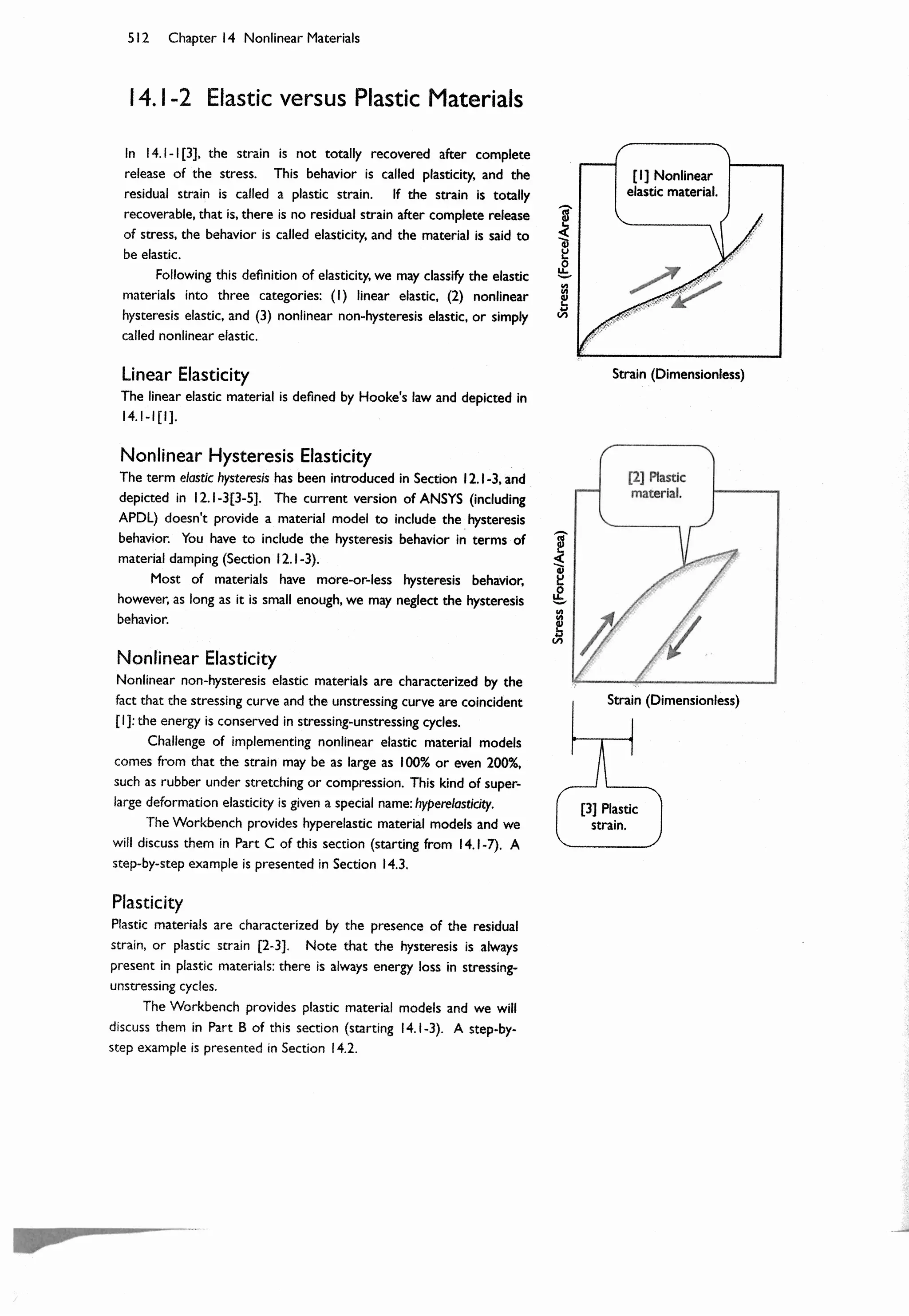
![Section 14.1 Basics of Nonlinear Materials 513
PART B. PLASTICITY
Stress(Force/Area)
Strain (Dimensionless)
Plasticity behavior typically occurs in ductile metals subject to large
deformation. Plastic strain results from slip between planes of atoms
due to shear stresses. This dislocation deformation is a
rearrangement of atoms in the crystal structure.
In the Workbench, a typical stress-strain relation, such as
14.1-2[2], is idealized to the one as shown [1-4]. The stress-strain
curve is composed of several straight segments. The slope of the
first segment is the Young's modulus [3]. When the stress is
released, the strain decreases with a slope equal to the Young's
modulus [4]. This implies that if the stress/strain state is on the first
segment, the behavior is elastic: no plastic strain remains after
releasing the stress. The point at the end of the first segment is
called elastic limit, or initial yield point. All points higher than the initial
yield point are called subsequent yield points, since they all represent
yielding state.
A stress-strain relation such as [1-4] is not sufficient to fully
define a plasticity behavior. There are other questions that must be
answered: (a) What is the yield criterion? (b) What is the hardening
rule?
14.1-3 Idealized Stress-Strain Curve for Plasticity
14.1-4 Yield Criteria
A stress-strain curve such as 14.1-3[1-4] is usually obtained by a uniaxial tensile test. It provides an initial yield
strength y
of uniaxial tensile test. In three-dimensional cases, the stress state is multiaxial. According to what
criteria can we say that a stress state reaches a yield state? The Workbench uses von Mises criterion (Section 1.4-5) as
the yield criterion, that is, a stress state reaches yield state when the von Mises stress e
is equal to the current
uniaxial yield strength y
, or
1
2 1 2( )
2
+ 2 3( )
2
+ 3 1( )
2
= y
(1)
The yielding initially occurs when y
= y
, and the "current" uniaxial yield strength y
may change subsequently. As
mentioned at the end of Section 1.4-5, when plotted in the 1 2 3
space, Eq. (1) is a cylindrical surface aligned
with the axis 1
= 2
= 3
and with a radius of 2 y
. It is called a von Mises yield surface [1]. If the stress state is
inside the cylinder, no yielding occurs. If the stress state is on the surface, yielding occurs. No stress state can exist
outside the yield surface. If the stress state is on the surface and the stress state continue to "push" the yield surface
outward, the size (radius) or the location of the yield surface will change. The rule that describes how the yield surface
changes its size or location is called a hardening rule.
The concept of yield surface is worth emphasis again. In a uniaxial test, we are talking about "yield points" in
stress axis. In a biaxial case, the yielding state form a "yield line," while in a 3D cases, the yielding state is a "yield
surface."
[1] Idealized
stress-strain
curve.[2] Initial
yield point.
[3] The stress-
strain relation is
assumed linear
beforeYield
point, and the
slope is the
Young's modulus.
[4] When the
stress is released,
the strain
decreases with a
slope equal to the
Young's modulus.](https://image.slidesharecdn.com/huei-huanglee-finiteelementsimulationswithansysworkbench12-2010-151020015452-lva1-app6892/75/Finite-Element-Simulations-with-ANSYS-Workbench-2012-310-2048.jpg)
![514 Chapter 14 Nonlinear Materials
1
2
3
1
= 2
= 3
14.1-5 Hardening Rules
Two hardening rules are implemented in the Workbench: (a) kinematic hardening, and (b) isotropic hardening. It should
be noted that, in metal plasticity, hardening behavior is often a mix-up of kinematic and isotropic. Since the Workbench
implements only two extremities, you have to choose either one that is suitable to describe your application.
Kinematic Hardening
The kinematic hardening assumes that, when a stress state continues to "push" a yield surface outward, the yield
surface will change its location, according to the "push direction," but preserve the size of the yield surface. In a
uniaxial test, It is equivalent to say that the difference between the tensile yield strength and the compressive yield
strength remains a constant of 2 y
[1].
Kinematic hardening is generally used for small strain, cyclic loading applications.
Stress
Strain
y
2 y
[1] This is a von Mises yield surface,
which is a cylindrical surface aligned
with the axis 1
= 2
= 3
and with a
radius of 2 y
, where y
is the
current yield strength.
[1] The kinematic
hardening assumes
that the difference
between tensile yield
strength and the
compressive yield
strength remains a
constant of 2 y
.](https://image.slidesharecdn.com/huei-huanglee-finiteelementsimulationswithansysworkbench12-2010-151020015452-lva1-app6892/75/Finite-Element-Simulations-with-ANSYS-Workbench-2012-311-2048.jpg)
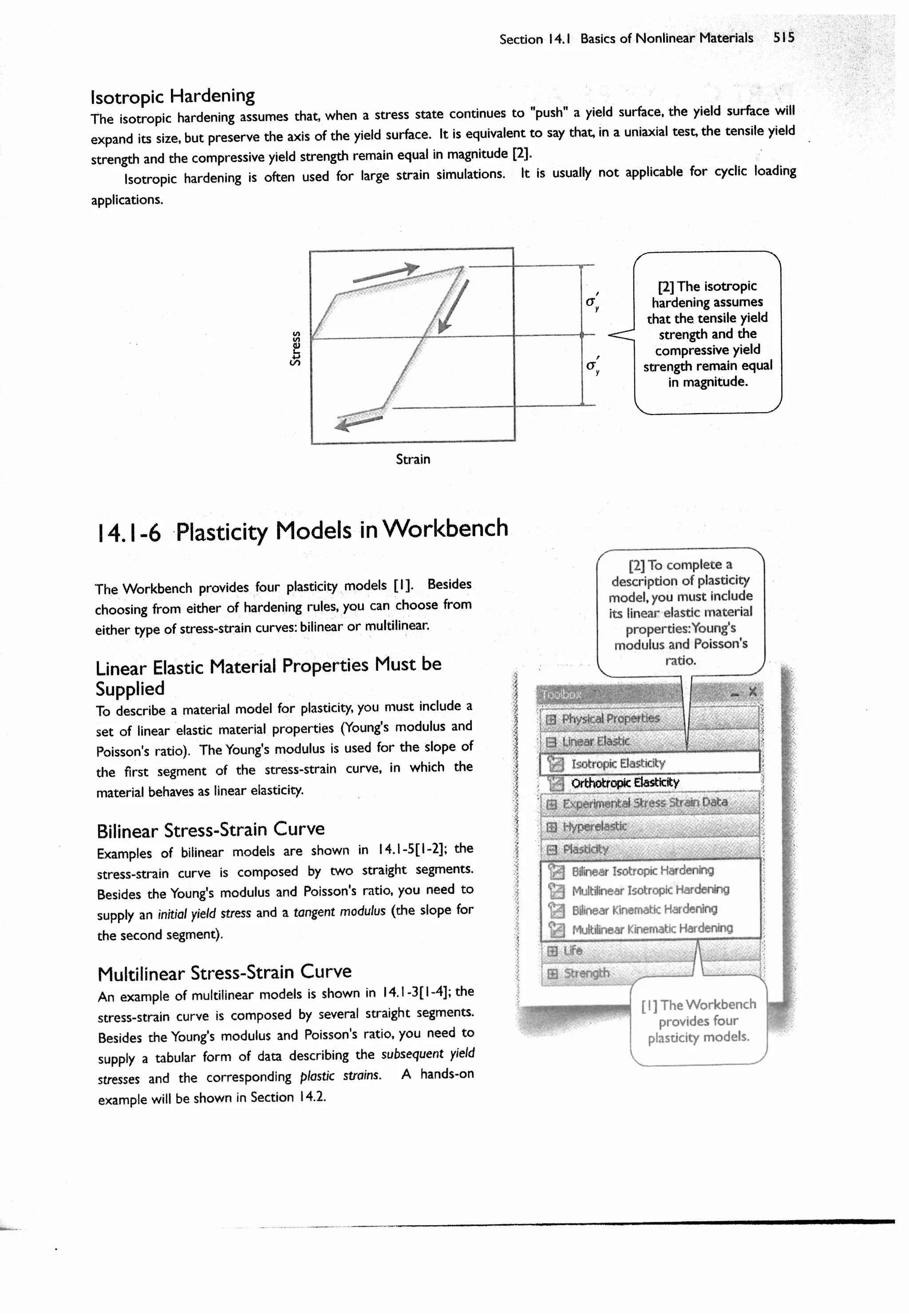
![516 Chapter 14 Nonlinear Materials
PART C. HYPERELASTICITY
14.1-7 Test Data Needed for Hyperelasticity
As mentioned in Section 14.1-2, challenge of implementing nonlinear elastic models comes from that the strain may be
as large as 100% or even 200%, such as rubber under stretching.
In plasticity or linear elasticity, we use a stress-strain curve to describe its behavior, and the stress-strain curve is
usually obtained by a tensile test. Since only tension behavior is investigated, other behaviors (compression, shearing)
must be drawn from the tensile test data. In plasticity or linear elasticity, we implicitly made some assumptions: (a) The
compressive behavior is symmetric to the tension behavior in the sense that they have the same Young's modulus, and
the same Poisson's ratio. The symmetry may not be true when the strain is large. We may need to conduct a
compressive test to assess the Young's modulus and the Poisson's ratio for the compressive behavior. (b) The shear
modulus G is related to theYoung's modulus and the Poisson's ratio by Eq. 1.2-8(2). Again, this assumption may not be
true when the strain is large. We may need to conduct a shear test to assess the shear modulus for describing the
shearing behavior. (c) We also assume that the bulk modulus B is related to the Young's modulus and the Poisson's
ratio by
B =
E
3(1 2 )
(1)
Again, this assumption may not be true when the strain is large. We may need to conduct a volumetric test to assess
the bulk modulus for describing the volumetric behavior. Note that, in many cases, the bulk modulus is almost
infinitely large (i.e., the material is incompressible). For these cases, we usually assume incompressibility without
conducting a volumetric test.
Further, when the strain is large, all the moduli (tensile, compressive, shear, and bulk) are no longer constant; they
change along stress-strain curves. Nonlinear elasticity with large strain is also called hyperelasticity.
As a summary, to describe hyperelasticity behavior, we need following test data: (a) a set of uniaxial tensile test
data, (b) a set of uniaxial compressive test data, (c) a set of shear test data, and (d) a set of volumetric test data if the
material is compressible.
Note that it is possible that a set of test data is obtained by superposing two sets of other test data. For
example, the set of uniaxial compressive test data can be obtained by adding a set of hydrostatic compressive test data
to a set of equibiaxial tensile test data [1-3]. Reasons of doing this are as follows. (a) Biaxial tesile test may be easier
to conduct than compressive test in some testing devices; (b) For incompressible materials, hydrostatic compressive
test data are trivial: all strains have zero values.
An example of test data for hyperelasticity is shown below [4-6], which will be used in of Section 14.3.
= +
[1] Uniaxial
compressive test.
[2] Equibiaxial
tensile test.
[3] Hydrostatic
compressive test.](https://image.slidesharecdn.com/huei-huanglee-finiteelementsimulationswithansysworkbench12-2010-151020015452-lva1-app6892/75/Finite-Element-Simulations-with-ANSYS-Workbench-2012-313-2048.jpg)
![Section 14.1 Basics of Nonlinear Materials 517
0
60
120
180
240
300
0 0.2 0.5 0.7
Stress(psi)
Strain (Dimensionless)
14.1-8 Strain Energy Function
Raw test data such as 14.1-7[4-6] are not convenient for internal calculations in the Workbench. It is usually preferable
to use mathematical forms to describe material behavior (such as Eq. 1.2-8(1)). The idea is to propose mathematical
forms with parameters, and determine the parameters that best-fit the test data.
Since there are three sets of test data, a rudimentary idea is to propose a mathematical form for each set of data.
This idea is not workable since, as discussed in Section 1.2, components of a stress state or a strain state are not
arbitrary values; they must satisfy some relations, such as Eq. 1.2-6(2). For example, given a strain state, it is possible to
look up the mathematical forms and obtain components of a "stress state," which is, however, not necessarily satisfy
the equilibrium relation (Eqs. 1.2-6(2) or 1.2-6(3)); the components may not be a "legal" stress state.
We need better ideas.
As mentioned in Section 14.1-2, hyperelasticity is characterized by the fact that the stressing curve and the
unstressing curve are coincident (14.1-2[1]): during the stressing and unstressing, the energy is conserved, or,
equivalently, the stressing and unstressing are path independent. The stress state depends only on the strain state, and
vice versa. They are independent of the stressing/unstressing history. This implies that there exists a potential energy
function that depends on the state of the stress or strain. It reminds us the strain energy density function W, which
does depend only on the state of stress or strain. We may propose a mathematical form for the strain energy
W = W( ij
) (1)
And the stress can be calculated from the strain energy using
ij
=
W
ij
(2)
The strain state ij
consists of 6 strain components (Eq. 1.2-4(4)). To further simply the strain energy function and
develop a coordinate-independent expression, we may replace the 6 strain components (which are coordinate-
dependent) with 3 strain invariants (which are coordinate-independent). To go further, we need more background.
Let's refresh some terms in solid mechanics.
[4] Uniaxial
test data.
[6] Shear test
data.
[5]
Equibiaxial test
data.](https://image.slidesharecdn.com/huei-huanglee-finiteelementsimulationswithansysworkbench12-2010-151020015452-lva1-app6892/75/Finite-Element-Simulations-with-ANSYS-Workbench-2012-314-2048.jpg)
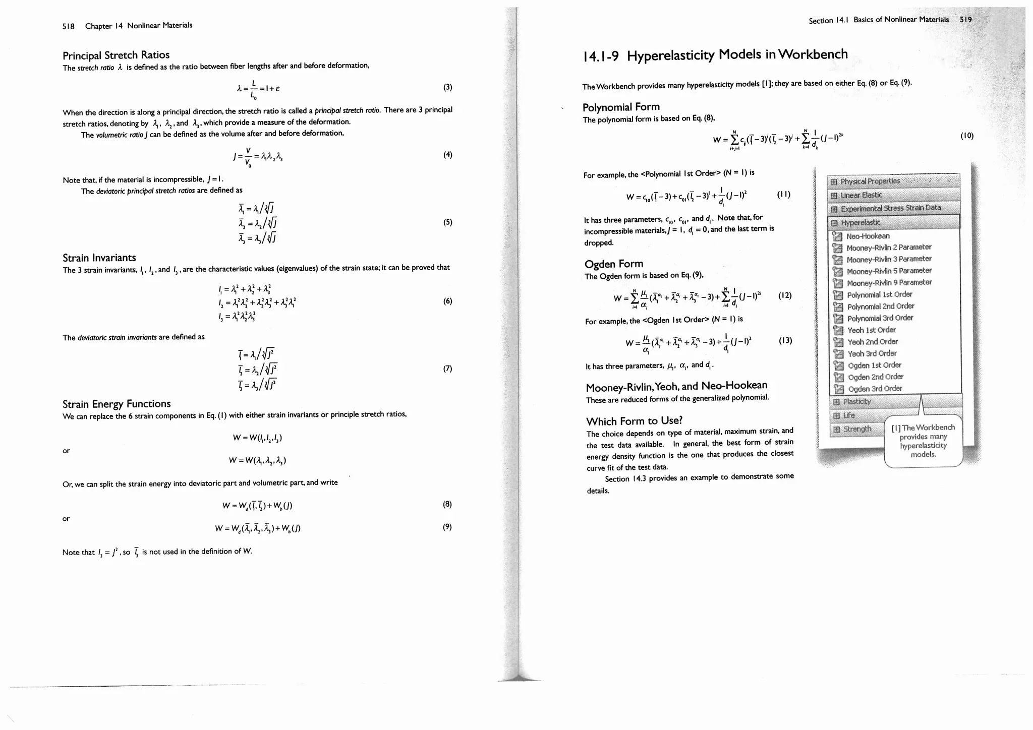
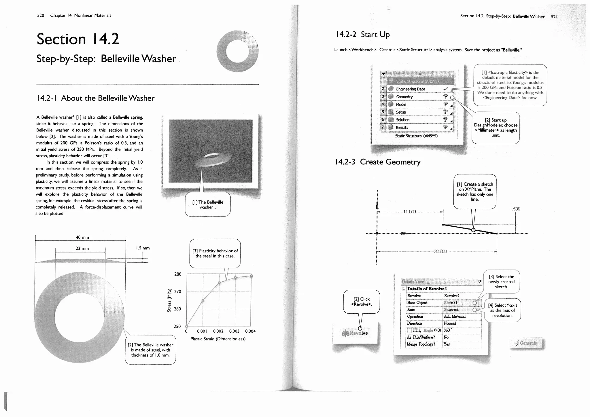
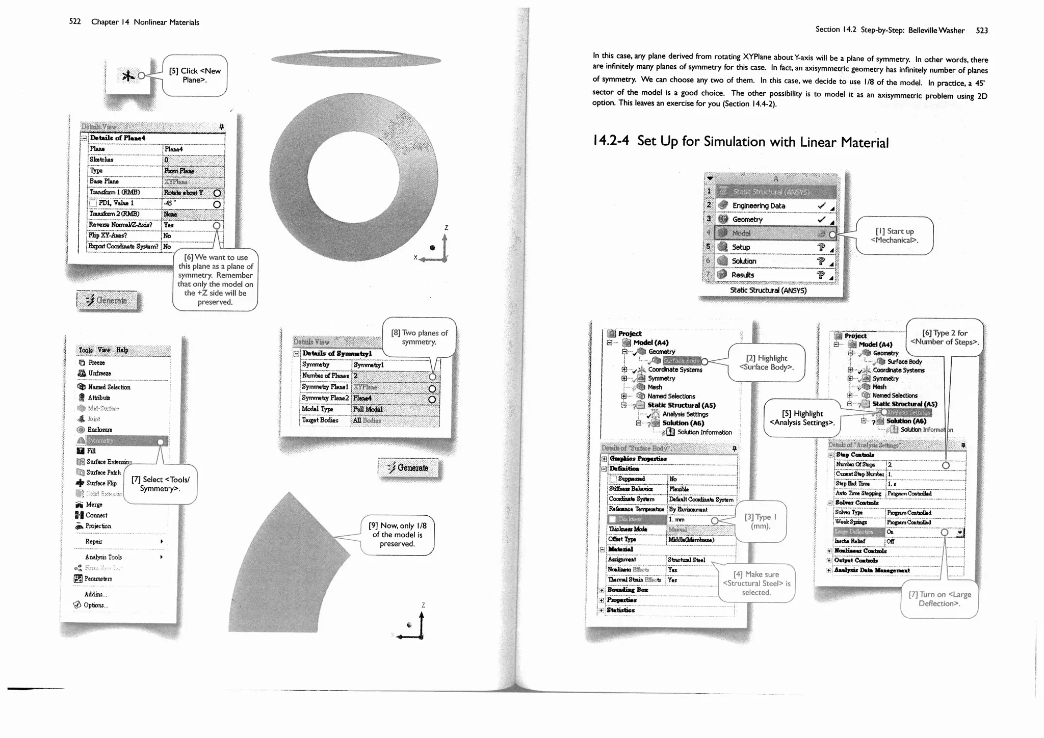
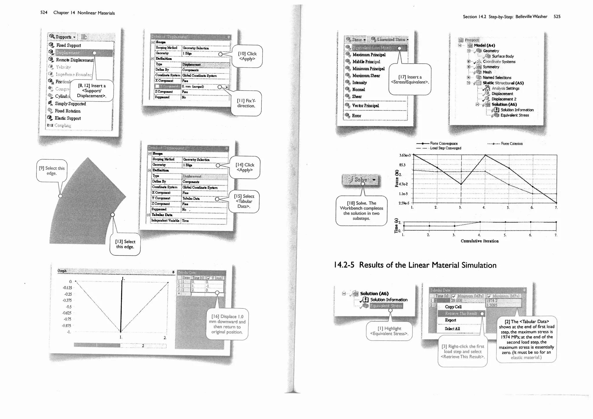
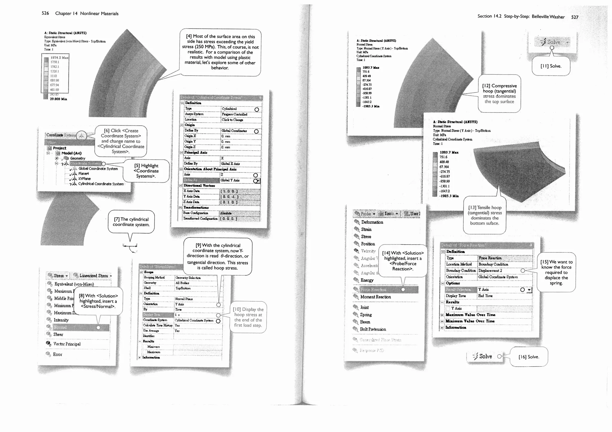
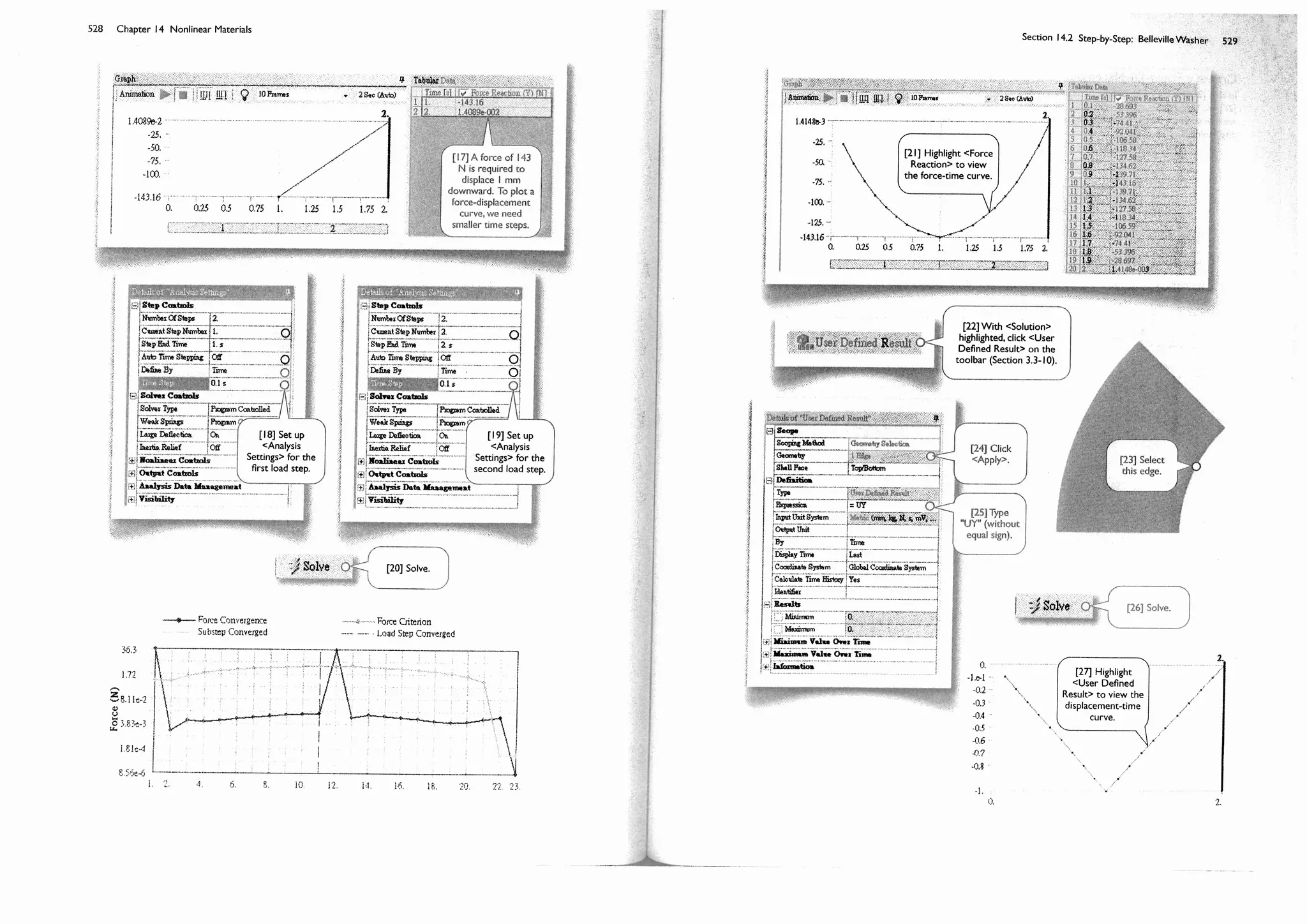
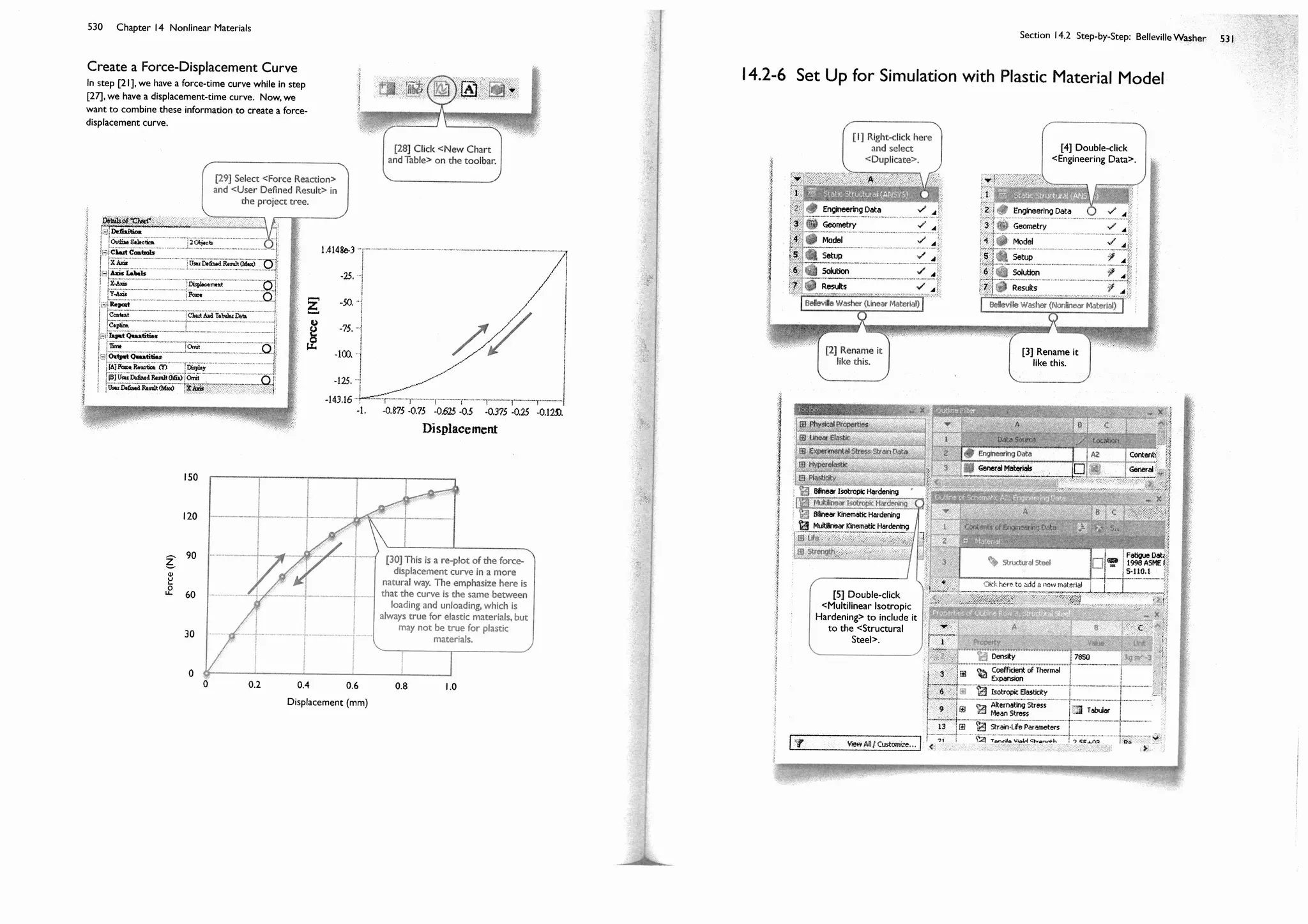
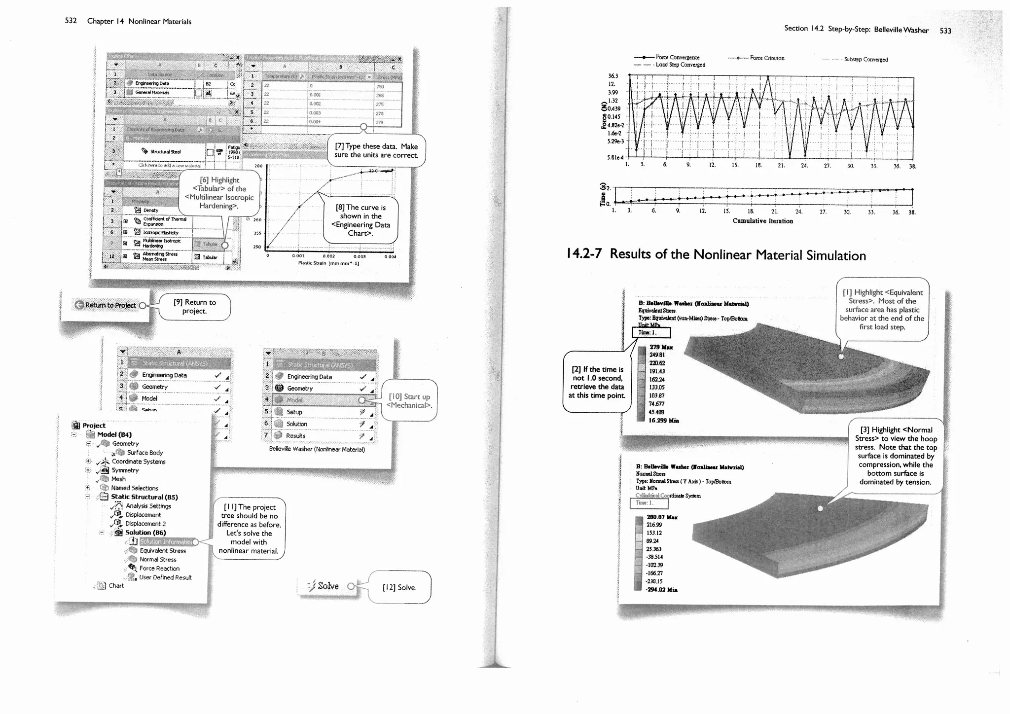
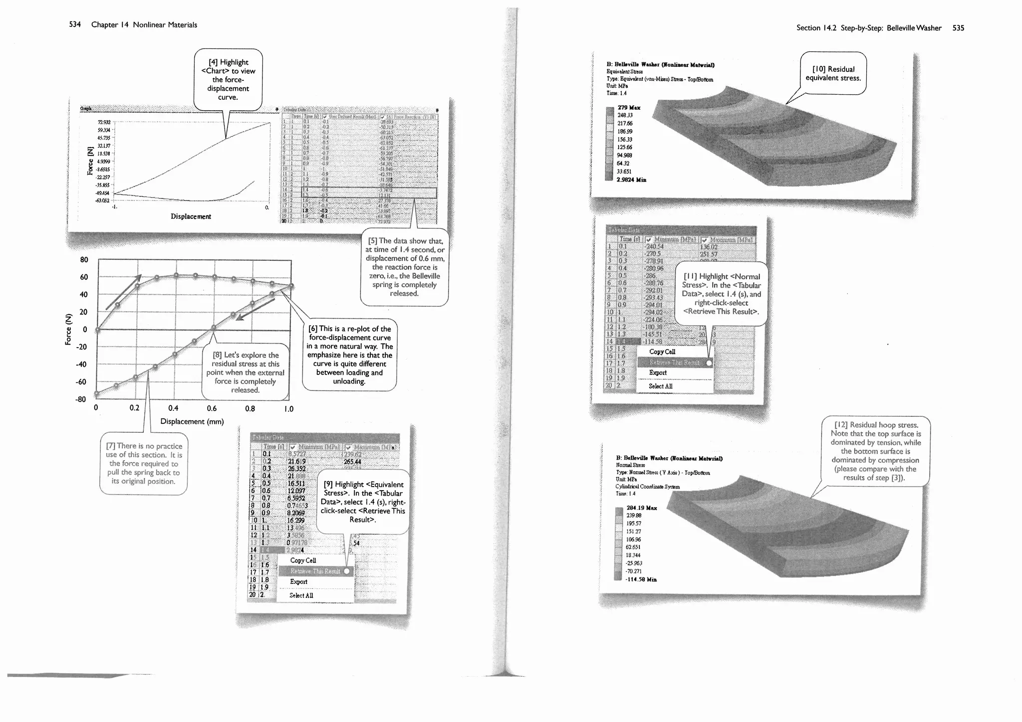
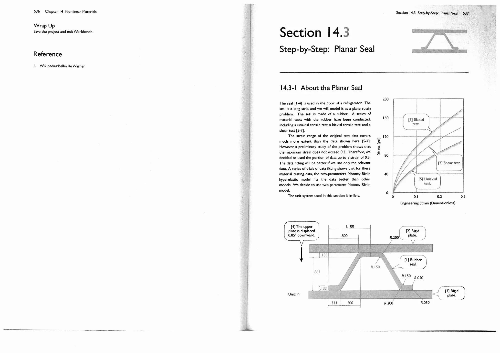
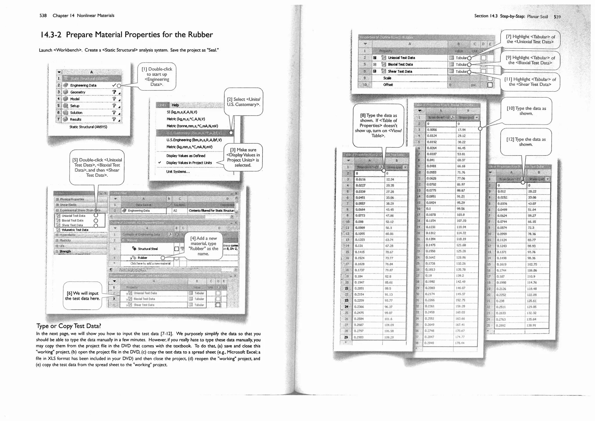
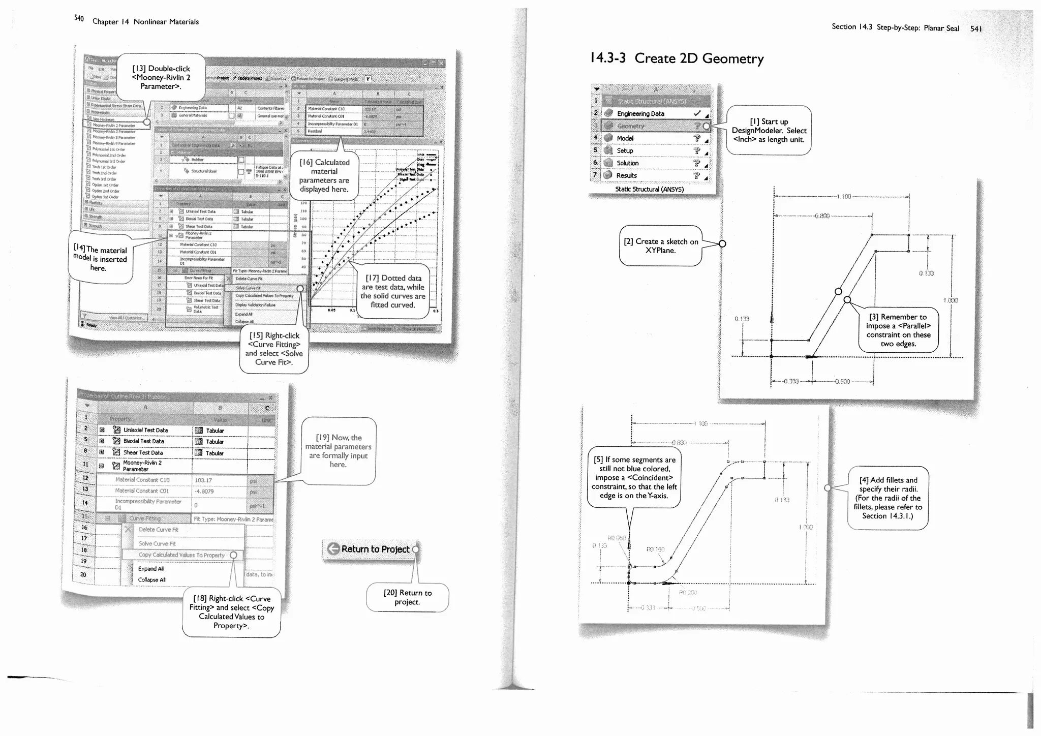
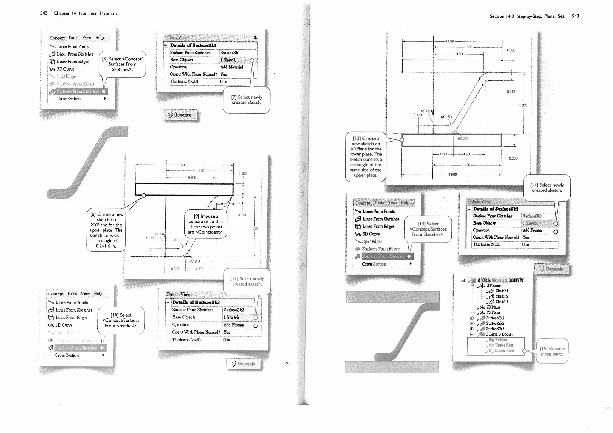

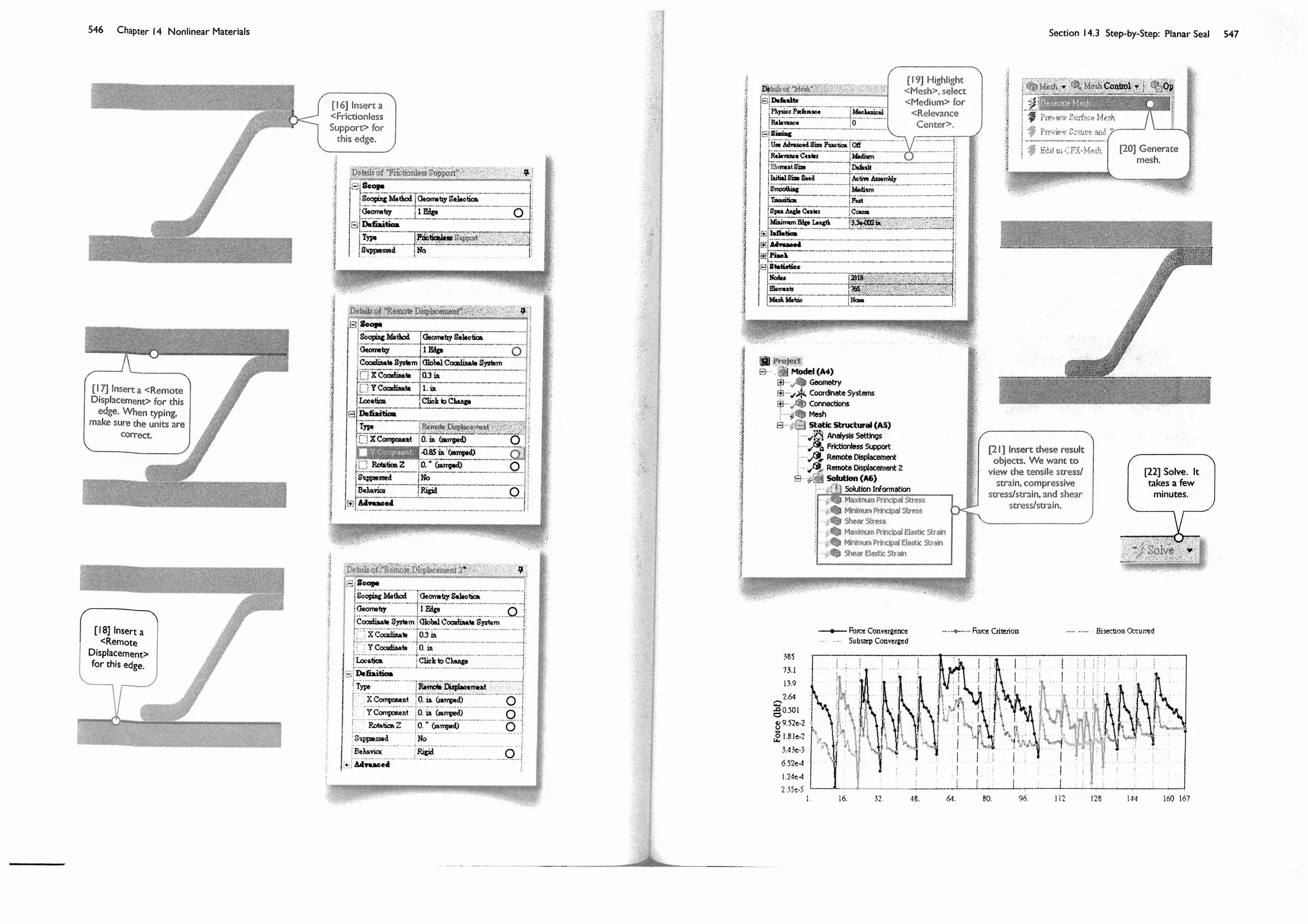
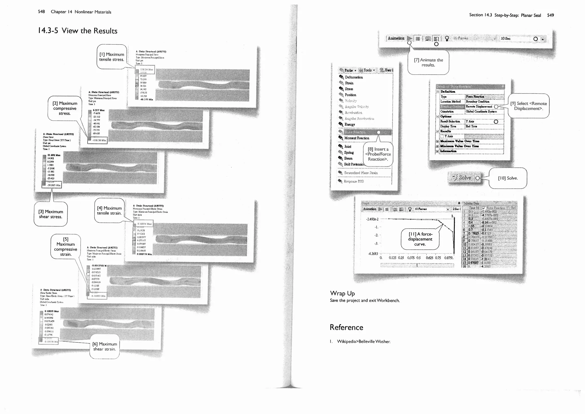
![Section 15.1 Basics of Explicit Dynamics 553
Section 15.1
Basics of Explicit Dynamics
15.1-1 Implicit Integration Methods
Consider solving Eq. 12.1-4(1) again,
M D{ }+ C D{ }+ K D{ }= F{ } Copy of 12.1-4(1)
Consider a typical time step t = tn+1
tn
. Let Dn
, Dn
, and Dn
be the displacement, velocity, and acceleration at tn
,
and Dn+1
, Dn+1
, and Dn+1
be those at tn+1
. Consider a special case that the acceleration is linear over the time step (i.e.,
Dn
= Dn+1
= 0 ), then, by Taylor series expansions at tn
,
Dn+1
= Dn
+ tDn
+
t2
2
Dn
(1)
Dn+1
= Dn
+ tDn
+
t2
2
Dn
+
t3
6
Dn
(2)
The quantity Dn
can be approached by
Dn
=
Dn+1
Dn
t
(3)
Substitution of Eq. (3) into Eqs. (1) and (2) respectively yields
Dn+1
= Dn
+
t
2
Dn+1
+ Dn( ) (4)
Dn+1
= Dn
+ tDn
+ t2 1
6
Dn+1
+
1
3
Dn
(5)
Eqs. (4) and (5) can be regarded as a special case of the Newmark method,
Dn+1
= Dn
+ t Dn+1
+ (1 )Dn
(6)
Dn+1
= Dn
+ tDn
+
1
2
t2
2 Dn+1
+ (1 2 )Dn
(7)
If you substitute =1 2 and =1 6 into Eqs. (6) and (7) respectively, you will obtain Eqs. (4) and (5).
Eqs. (6) and (7) are used in <Transient Structural> analysis system. The parameters and are chosen to
control characteristics of the algorithm such as accuracy, numerical stability, etc. It is called an implicit method because
the calculation of Dn+1
and Dn+1
requires knowledge of Dn+1
. That is, the response at the current time step depends on
not only the historical information but also the current information; iterations are needed to solve Eqs. (6) and (7).
Calculation of the response at time tn+1
is conceptually depicted in [1-6]. In the beginning [1], the displacement
Dn
, velocity Dn
, and acceleration Dn
of the last step are already known (For n = 0, we may assume D0
= 0 ). Since
Dn+1
is needed in Eqs. (6) and (7), we use Dn
as an initial gauss of Dn+1
. Knowing Dn
, Dn
, and Dn+1
, the quantities Dn+1
and Dn+1
can be calculated according to Eqs. (6) and (7) [2]. The next step [3] is to substitute Dn+1
, Dn+1
, and Dn+1
into
Eq. 12.1-4(1). If Eq. 12.1-4(1) is satisfied, then the calculation of the response at time tn+1
is complete [5], otherwise,
Dn+1
is updated and another iteration is initiated [6]. Update of Dn+1
[6] is similar to the Newton-Raphson method
described in Section 13.1-4.](https://image.slidesharecdn.com/huei-huanglee-finiteelementsimulationswithansysworkbench12-2010-151020015452-lva1-app6892/75/Finite-Element-Simulations-with-ANSYS-Workbench-2012-333-2048.jpg)
![554 Chapter 15 Explicit Dynamics
Yes
No
[1] Given the response of the
last step, Dn
, Dn
, and Dn
. Use
Dn
as an initial gauss of Dn+1
.
[2] Calculate Dn+1
and Dn+1
,
according to Eqs. (6) and (7).
[3] Substitute Dn+1
, Dn+1
, and
Dn+1
into Eq. 12.1-4(1).
[4] Eq.
12.1-4(1)
satisfied?
[5] Response of the "current"
step becomes that of the "last
step."
[6] Update Dn+1
.
15.1-2 Explicit Integration Methods
The explicit method used in <Explicit Dynamics> analysis system is based on half-step central differences
Dn
=
Dn+1
2
Dn 1
2
t
, or Dn+1
2
= Dn 1
2
+ Dn
t (1)
Dn+1
2
=
Dn+1
Dn
t
, or Dn+1
= Dn
+ Dn+1
2
t (2)
Eqs. (1) and (2) are called explicit methods because the calculation of Dn+1
2
and Dn+1
requires knowledge of historical
information only. That is, the response at the current time can be calculated explicitly; no iterations within a time step
is needed. Therefore, it is very efficient to complete a time step, also called a cycle. One of the distinct characteristics
of the explicit method is that its integration time step needs to be very small in order to achieve an accurate solution.
With implicit methods, a typical integration time step is about 0.0001 to 0.01 seconds; a typical simulation time is
about 0.1 to 10 seconds, which involves hundreds or thousands of integration time steps.
Implicit methods can be used for most of transient structural simulations. However, for highly nonlinear
problems, it often fails due to convergence issues; for high-speed impact problems, the integration time is so small that
the computing time becomes intolerable. In such cases, explicit methods are more applicable.](https://image.slidesharecdn.com/huei-huanglee-finiteelementsimulationswithansysworkbench12-2010-151020015452-lva1-app6892/75/Finite-Element-Simulations-with-ANSYS-Workbench-2012-334-2048.jpg)
![Section 15.1 Basics of Explicit Dynamics 555
[1] Given the initial
conditions, D0
and D0
.
Set n = 0.
[3] Calculate element
strains and strain rates.
[5] Calculate element
stresses.
[6] Calculate nodal
forces.
[7] Calculate nodal
accelerations Dn
.
[8] Calculate nodal
velocity Dn+1
2
.
[9] Calculate nodal
displacements Dn+1
.
This completes a cycle.
Set n = n + 1.
[2] Given Dn
and Dn
.
[4] Calculate element
volume changes and
update their mass
density.
The procedure used in the <Explicit Dynamics> analysis system is illustrated in [1-9]. In the beginning of a cycle
[2], the displacement Dn
and velocity Dn
of the last cycle are already known. With these information, we can calculate
the strain and strain rate for each element [3], using the relations such as Eqs. 1.3-2(2) and 1.2-7(1). The volume
change for each element is then calculated, according to the equations of state, and the mass density is updated [4].
The volumetric information is needed for the calculation of stresses. With these information, the element stresses can
be calculated [5] according to a constitutive model, relation between stresses and strains/strain rates, such as Eq.
1.2-8(1). The stresses are integrated over the elements, and the external loads are added to form the nodal forces Fn
[6]. The nodal accelerations are then calculated [7] according to
Dn
=
Fn
m
+
b
(3)
where b is the body force (see Eq. 1.2-6(2)), m is the nodal mass, and is the mass density. The nodal velocities at
tn+1
2
are calculated [8] according to Eq. (1) and the nodal displacements at tn+1
are calculated [9] according to Eq. (2).
With explicit methods, a typical integration time step is about 1 nanosecond to 1 microsecond; a typical
simulation time is about 1 millisecond to 1 second, which will need many thousands or millions of cycles.
Explicit methods is useful for high-speed impact problems and highly nonlinear problems. For low-speed
problems, using explicit methods becomes impractical due to an enormous computing time, since it requires very small
integration time steps.](https://image.slidesharecdn.com/huei-huanglee-finiteelementsimulationswithansysworkbench12-2010-151020015452-lva1-app6892/75/Finite-Element-Simulations-with-ANSYS-Workbench-2012-335-2048.jpg)
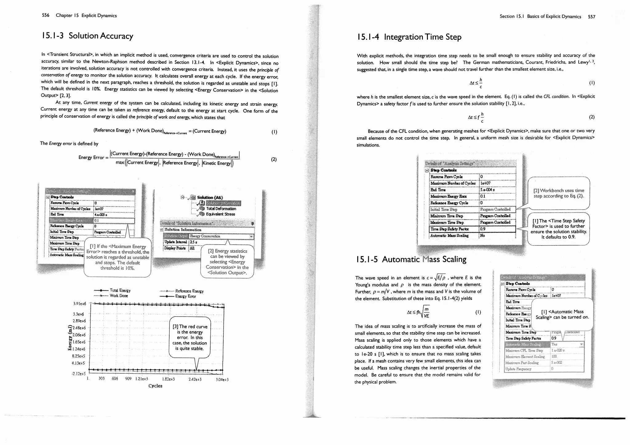
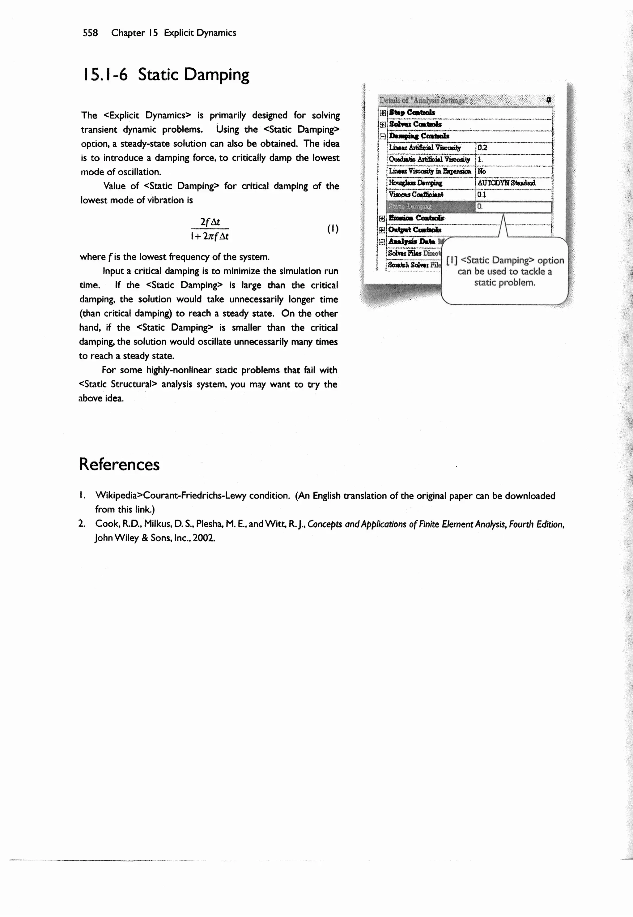
![Section 15.2 Step-by-Step: High-Speed Impact 559
Section 15.2
Step-by-Step: High-Speed Impact
Imagine, during an explosion, an aluminum pipe that was blasted away under the explosive pressure. The pipe hit a
steel solid column, deformed, and finally torn to fragments due to excessive strain [1-6]. In this section, we will
demonstrate the simulation of this scenario. We will use the default settings as much as possible to demonstrate that
a complicated simulation like this can be done in <Explicit Dynamic> analysis system with just a few input data.
Both the aluminum pipe and the steel solid column have a diameter of 50 mm and a length of 200 mm. The steel
column is modeled as a rigid body and fixed in the space. The aluminum pipe has a thickness of 1 mm and, when
hitting the pipe, has a speed of 300 m/s (about the speed of sound). The aluminum is modeled as a bilinear isotropic
plasticity material (Section 14.1) using the material parameters stored in the <Engineering Data> with a modification
that the tangent modulus is set to zero, i.e., the aluminum is modeled as a perfectly elastic-plastic material. To simulate
the fragmentation, it is assumed that the aluminum will be torn apart (failed) when the plastic strain is larger than 75%.
The millimeter will be used to create the geometry and the MKS or SI unit systems will be used in the
simulation.
15.2-1 About the High-Speed Impact Simulation
[1] Time = 0. [2] Time = 0.0001 s.
[3] Time = 0.0002 s.
[4] Time =
0.0003 s.
[5] Time =
0.0004 s.
[6] Time = 0.0005 s.](https://image.slidesharecdn.com/huei-huanglee-finiteelementsimulationswithansysworkbench12-2010-151020015452-lva1-app6892/75/Finite-Element-Simulations-with-ANSYS-Workbench-2012-338-2048.jpg)
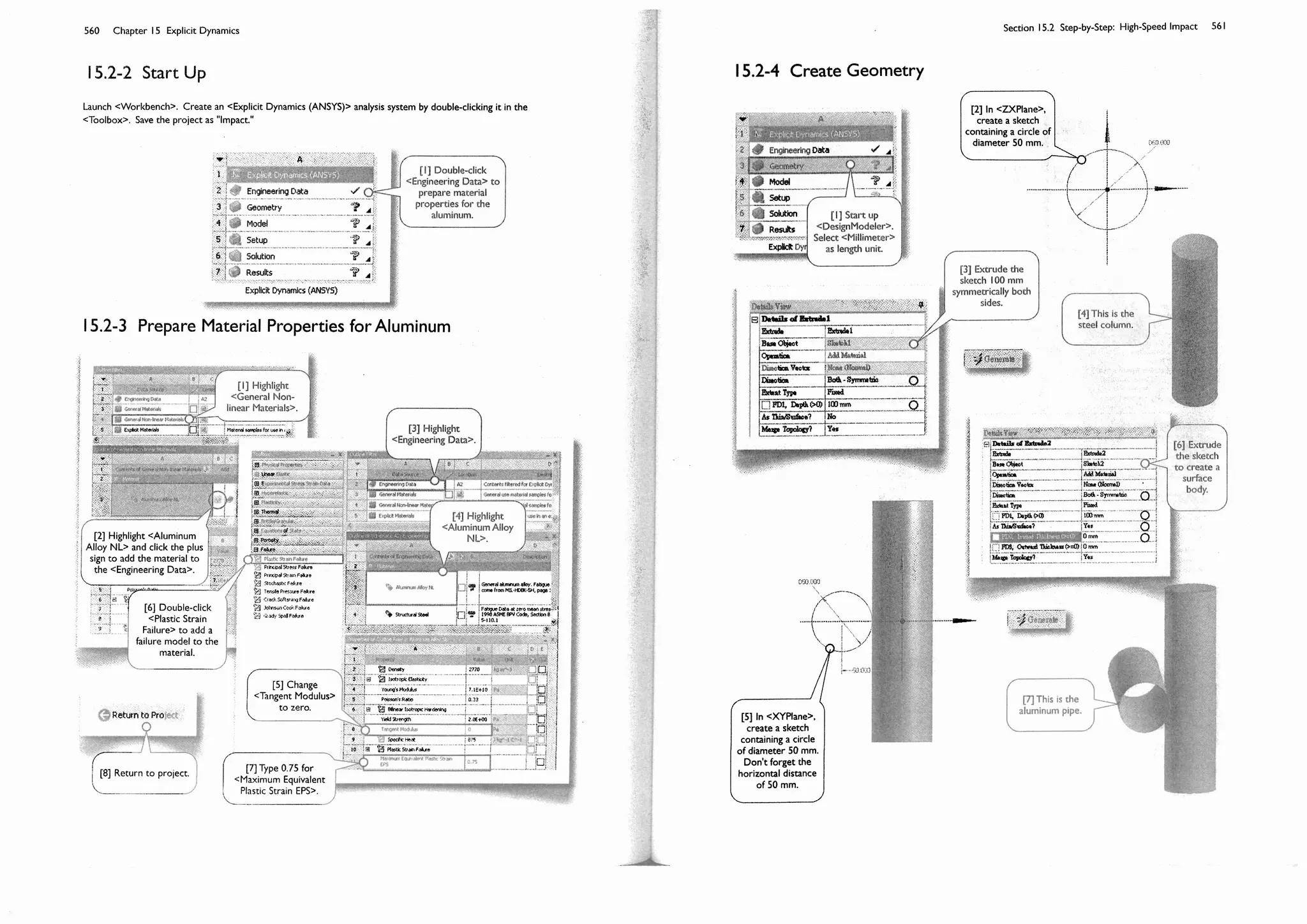
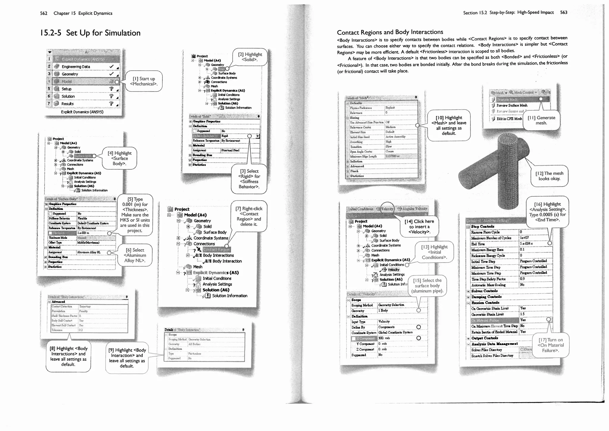
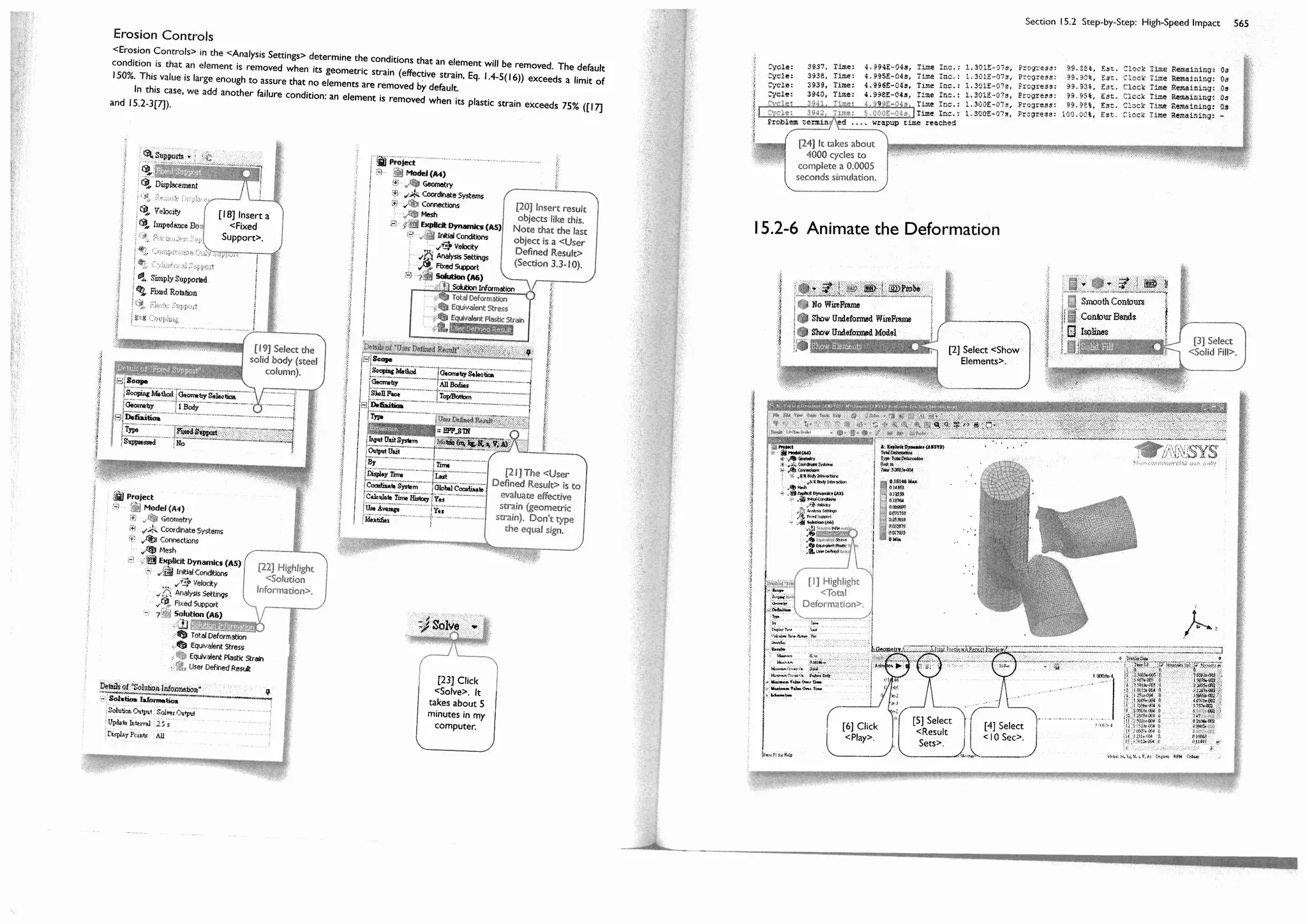
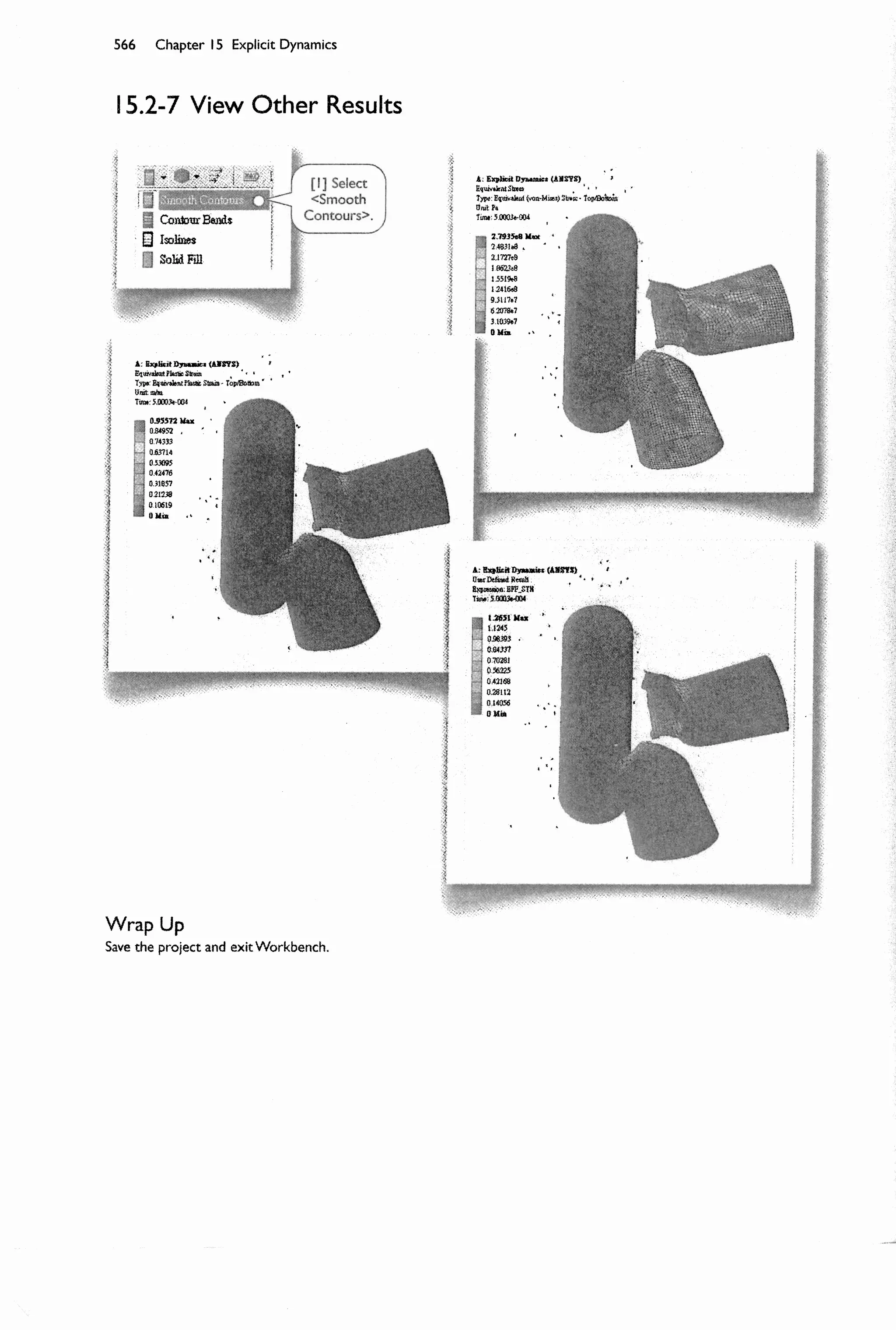
![Section 15.3 Step-by-Step: Drop Test 567
10
R3
20
5 m/s
60
120
R20
Section 15.3
Step-by-Step: Drop Test
Drop test simulation is a special case of impact simulation, in which one of the impacting objects is a stationary floor,
typically made of concrete, steel, or stone. In this section, we will simulate a scenario that a mobile phone falls off
from your pocket and drops on a concrete floor. This kind of simulations typically take hours of computing time.
From the experience of Section 15.2, a typical integration time step in <Explicit Dynamics> is 10 7
to 10 8
seconds. It
would take about 100,000 to 1000,000 cycles to complete a 0.01 seconds of drop test. In this section, we will simplify
the model to shorten the run time. A more realistic model will be suggested and leave for the students as an exercise
(Section 15.4-2).
The phone body is a shell of thickness 0.5 mm and made of an aluminum alloy [1]. The concrete floor is
modeled as an 160x40x10 (mm) block [2]. When the phone hits the floor, its velocity is 5 m/s, which is equivalent to a
free fall from a height of 1.25 m. We will assume that the phone body forms an angle of 20 with the horizon when it
hits the floor.
We will use the kg-mm-s-N unit system in both <DesignModeler> and <Mechanical>.
15.3-1 About the Drop Test Simulation
Unit: mm.
[1] The phone
body is made of an
aluminum alloy.
[2] The concrete floor can be
modeled with arbitrary sizes,
we will use 160x80x10 (mm).](https://image.slidesharecdn.com/huei-huanglee-finiteelementsimulationswithansysworkbench12-2010-151020015452-lva1-app6892/75/Finite-Element-Simulations-with-ANSYS-Workbench-2012-343-2048.jpg)
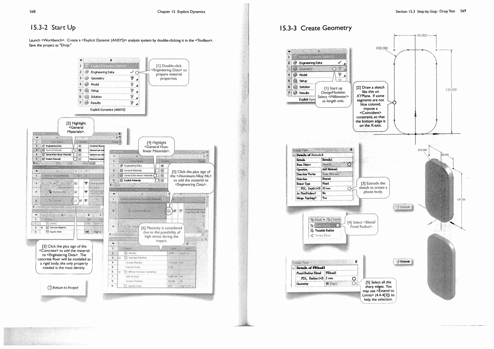
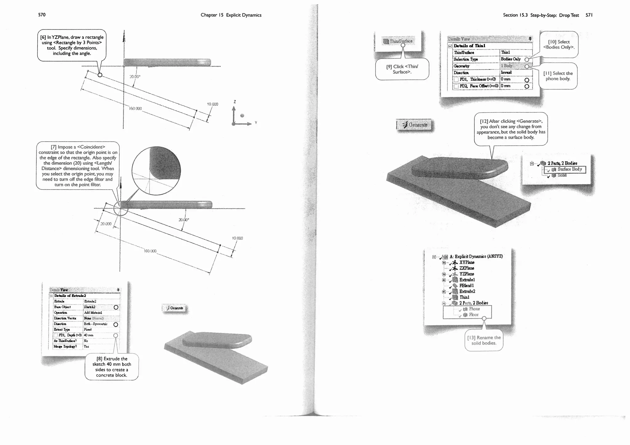
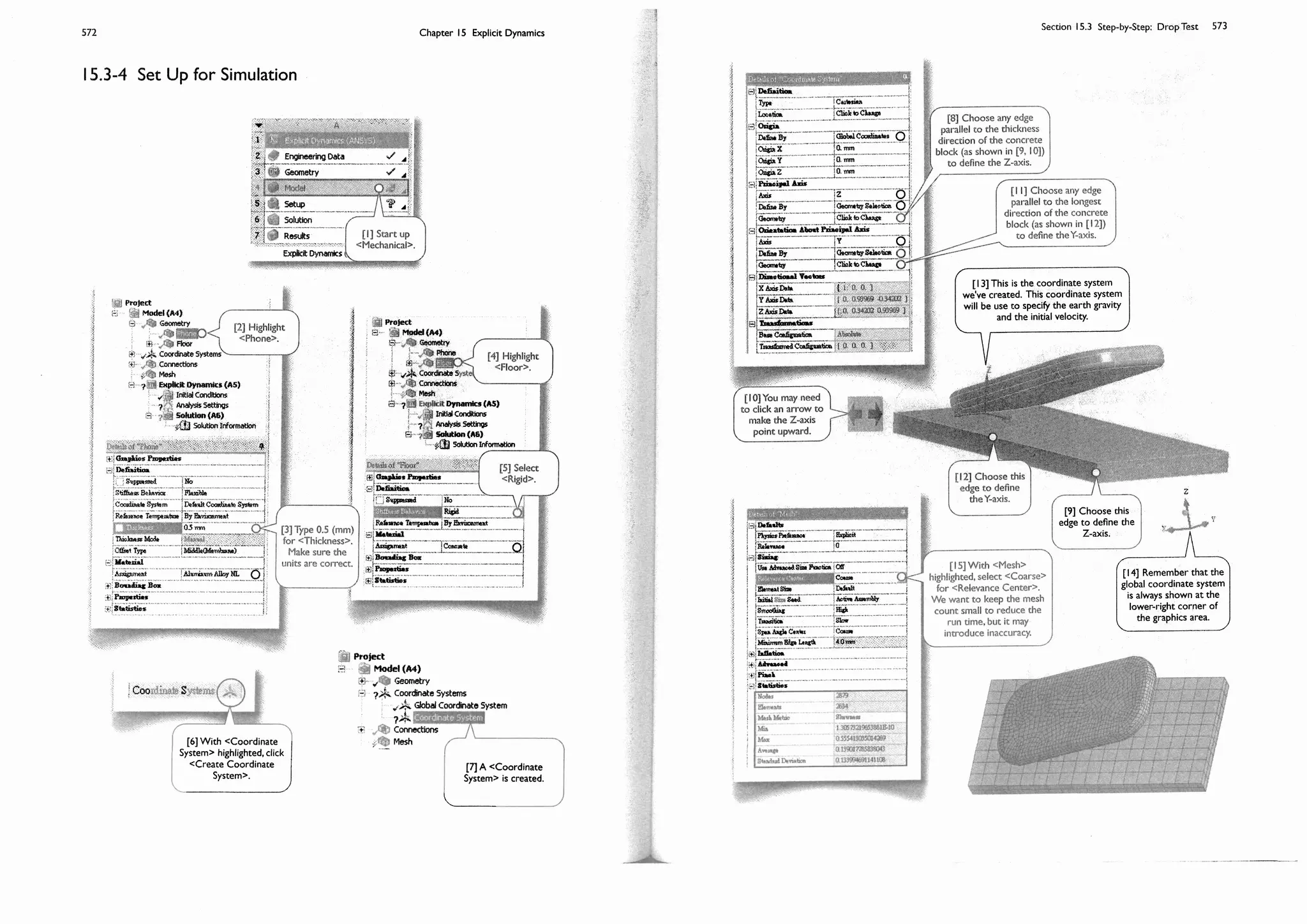
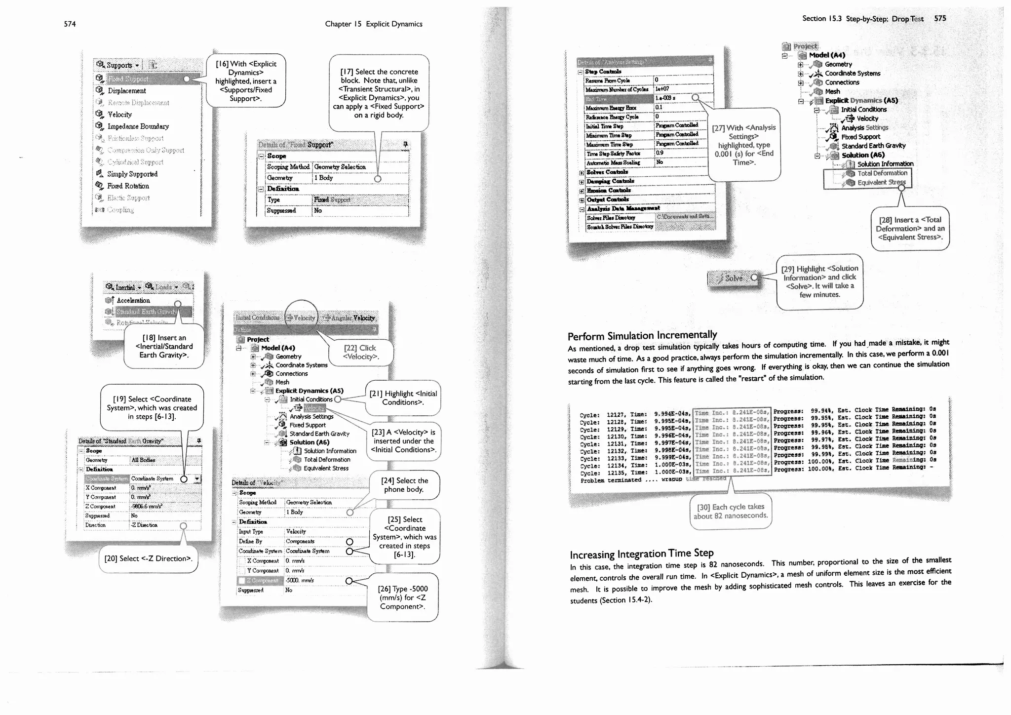
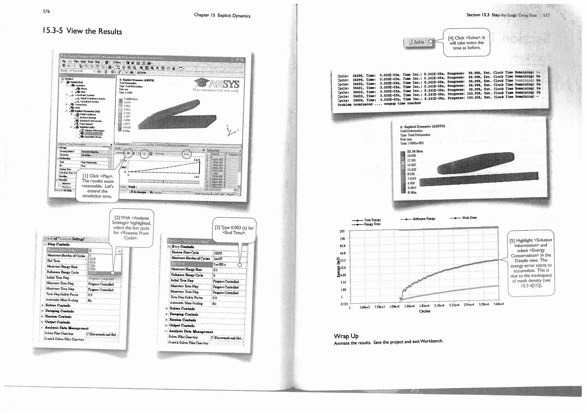


This document provides an overview and table of contents for a textbook on finite element simulations using ANSYS Workbench 12. The textbook is intended for graduate students and senior undergraduates. It uses real-world case studies and step-by-step exercises to teach various finite element analysis techniques, including linear static analysis, optimization, buckling, dynamics, nonlinear analysis, and explicit dynamics. Each chapter builds upon the previous chapters and introduces new simulation capabilities or analysis types. The goal is to provide students with a comprehensive yet accessible introduction to finite element analysis using ANSYS Workbench.