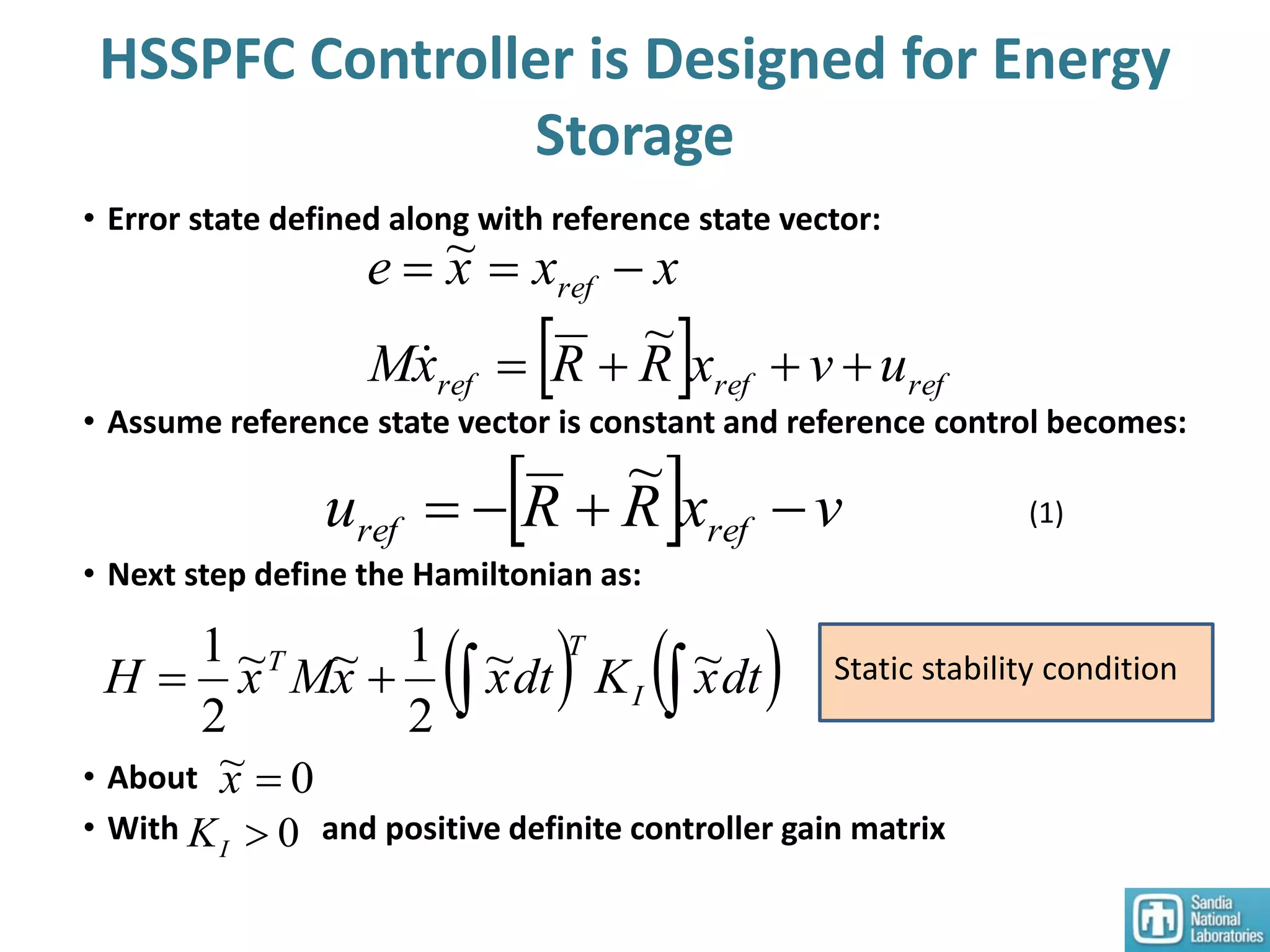
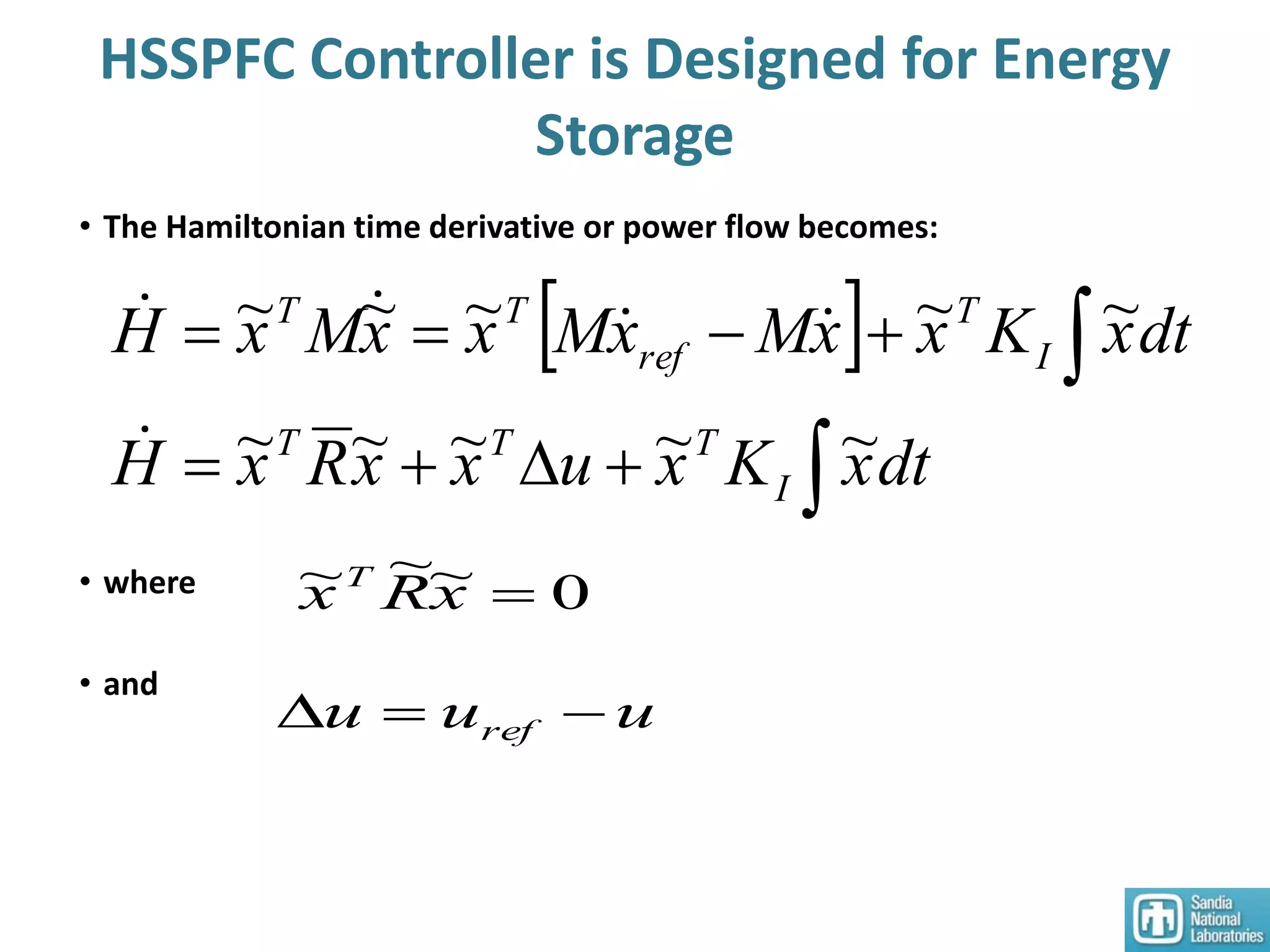
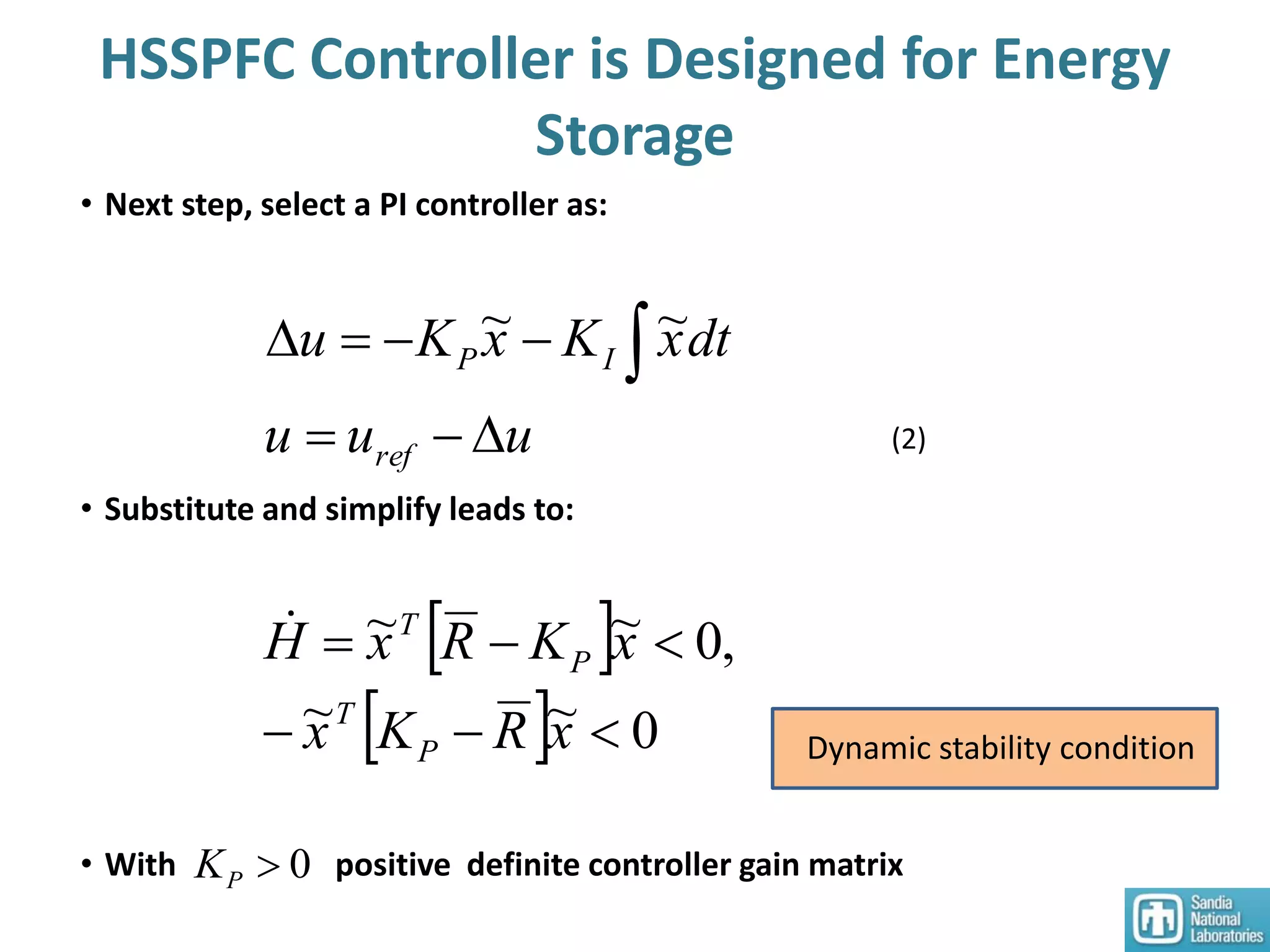
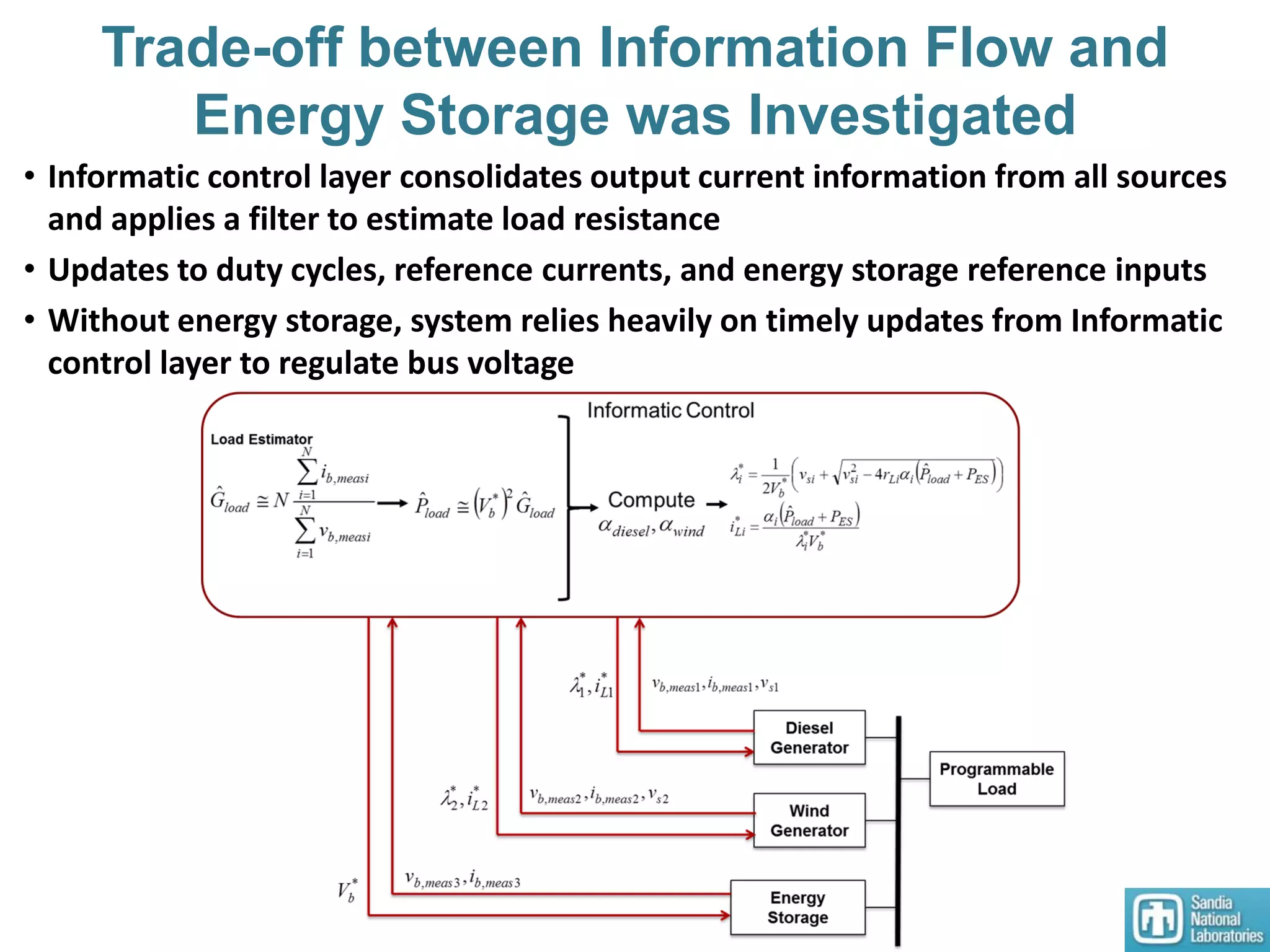
Download as PDF, PPTX

![A Path From Today’s Grid To The
Future (Smart) Grid
• Large spinning machines → Large inertia (matrix); dispatchable
supply with storage
• Constant operating conditions → well-ordered state
• Well-known load profiles → excellent forecasting
[I]ẋ=f(x,u,t) ; [I]-1 ~ [0] → ẋ=[I]-1 f(x,u,t) ~ 0 ; x(t)=x0
G-L>0 vt
Today’s Grid
Retain Today’s Grid: Replace lost storage with
serial or parallel additional energy storage](https://image.slidesharecdn.com/rt155davidwilsonsandia-150529190043-lva1-app6892/75/RT15-Berkeley-Optimized-Power-Flow-Control-in-Microgrids-Sandia-Laboratory-33-2048.jpg)
![A Path From Today’s Grid To The
Future (Smart) Grid (cont.)
Future Grid:
1. High penetration of renewables: loss of storage
Loss of large spinning machines
Loss of dispatchable supplies
2. Variable operating conditions → variable state x(t)=?
3. Stochastic load profiles → renewables as negative loads
[IF] ẋ = fF(x,u,t) → ẋF(t) = [IF]-1 fF(x,u,t)
G-L<0 much of the time
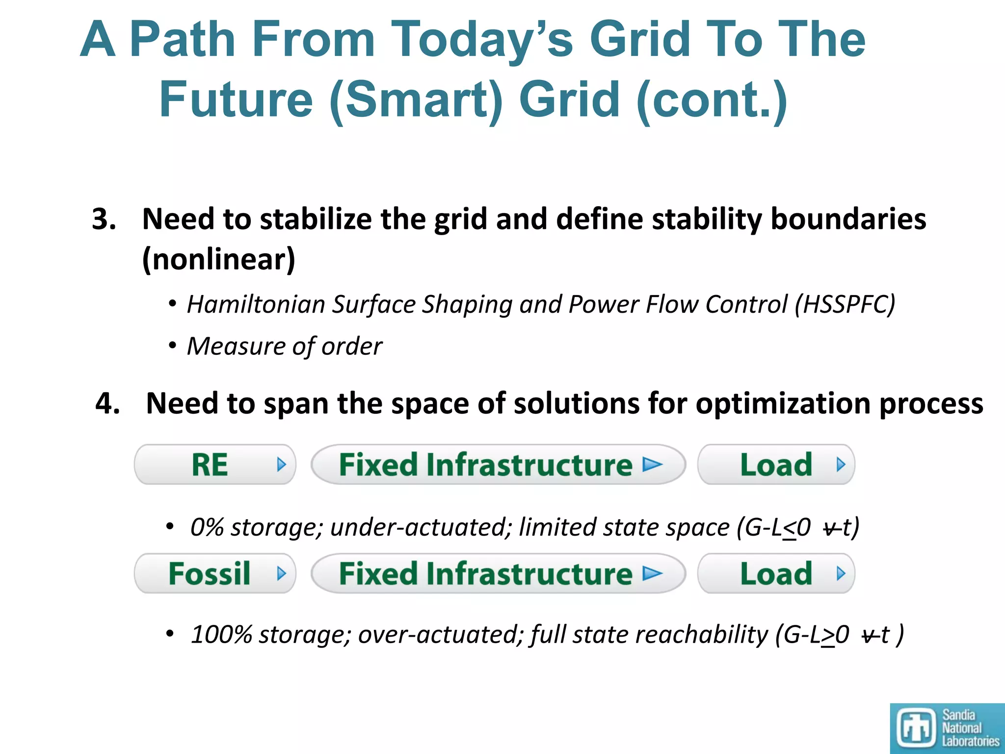
4. Problem Restated: How do we regain
a) Well-ordered state → x(t) ?
b) Well-known load profiles?
c) Dispatchable supply with energy storage?
d) Stability and performance?
e) An optimal grid?](https://image.slidesharecdn.com/rt155davidwilsonsandia-150529190043-lva1-app6892/75/RT15-Berkeley-Optimized-Power-Flow-Control-in-Microgrids-Sandia-Laboratory-34-2048.jpg)
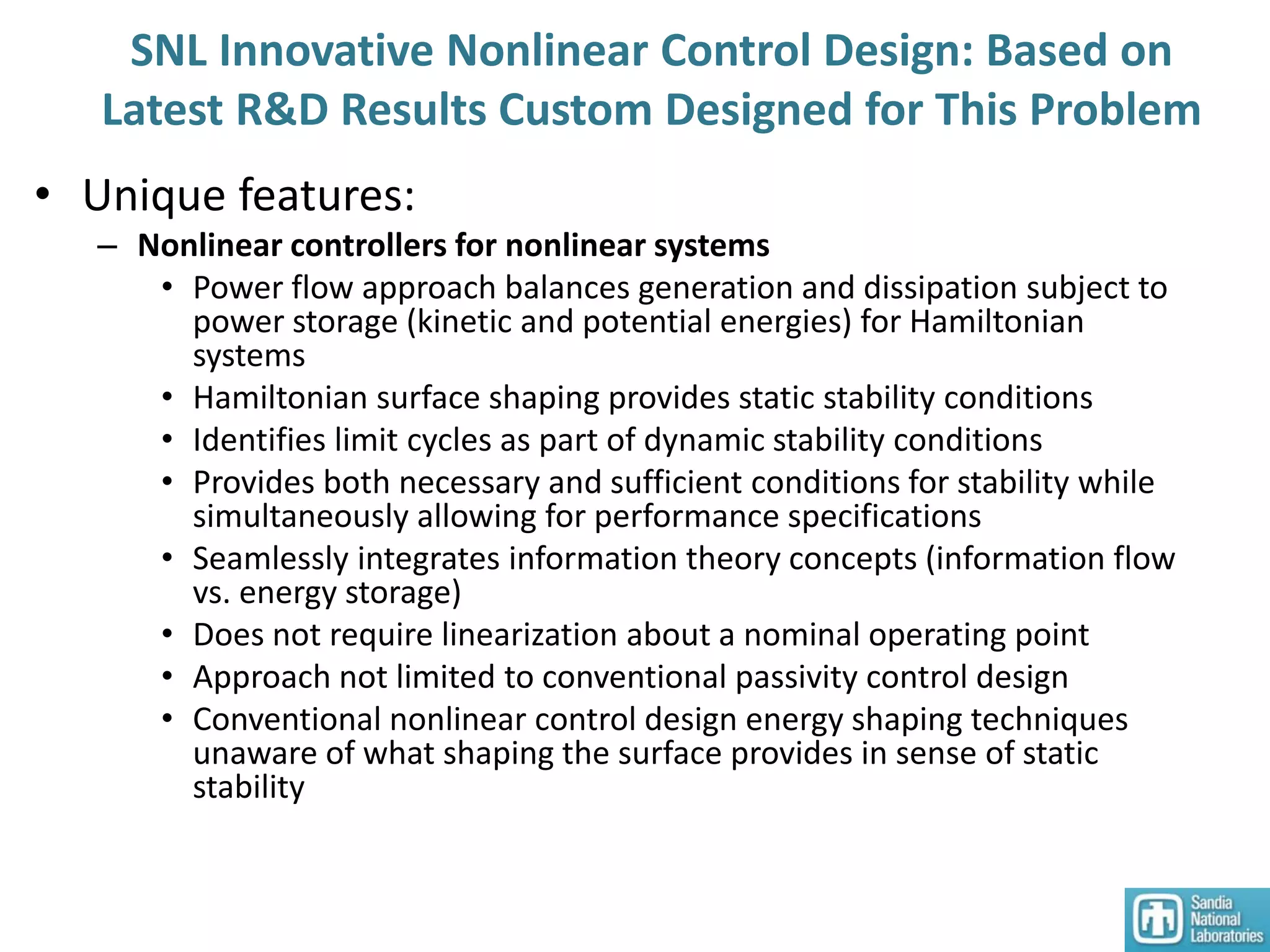
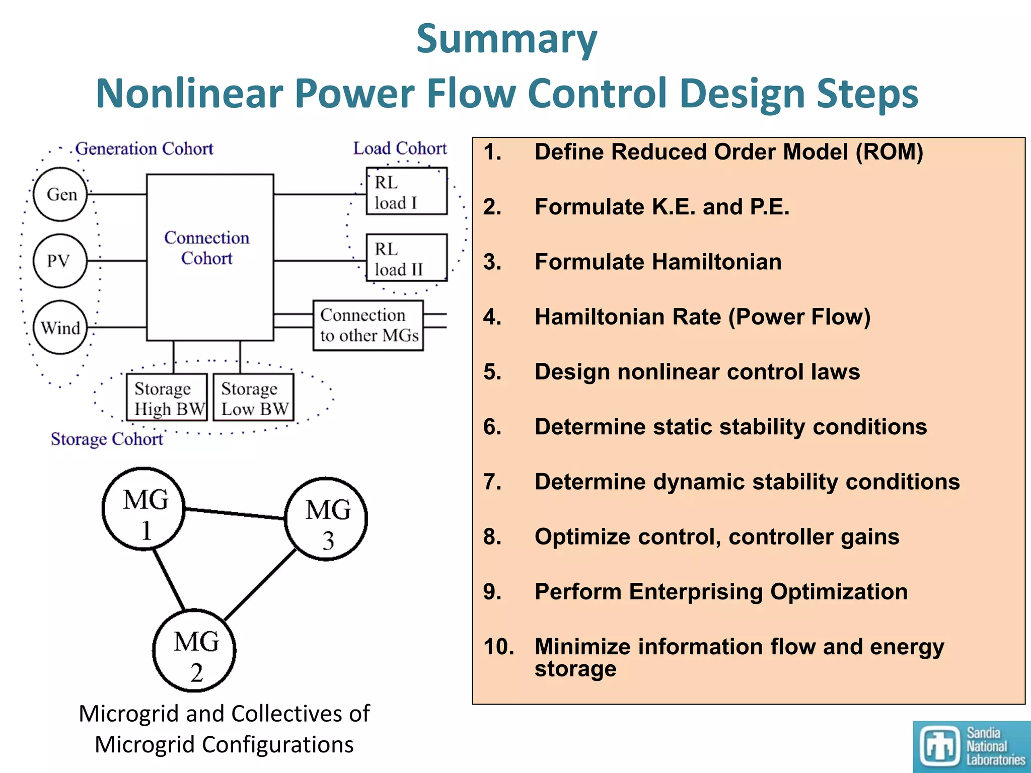
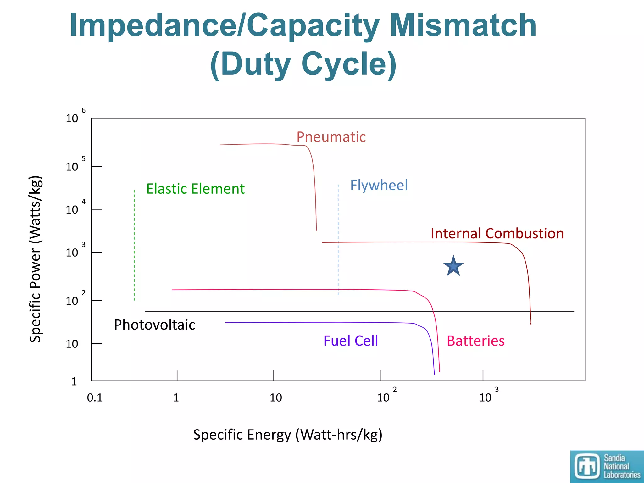

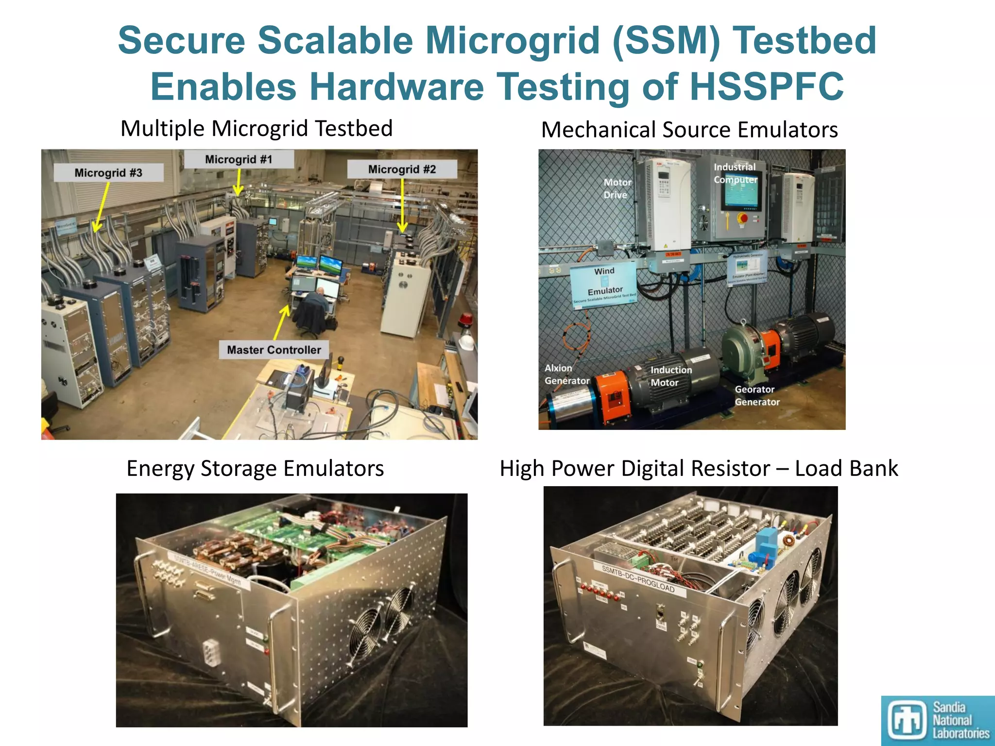
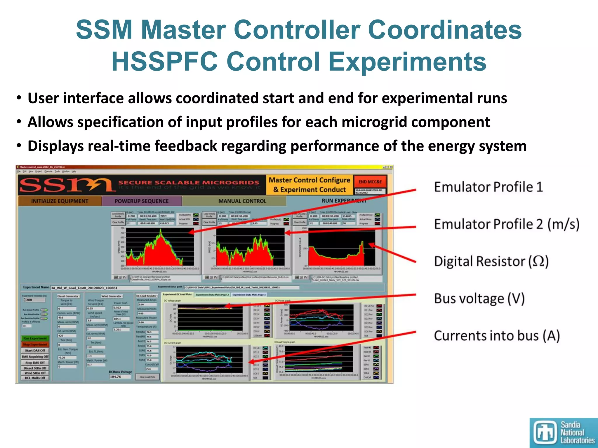
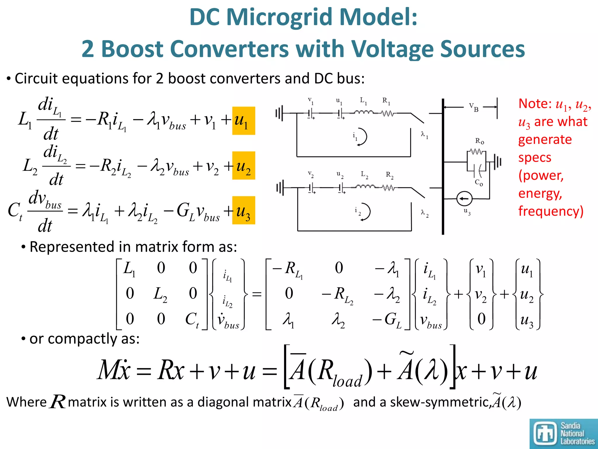
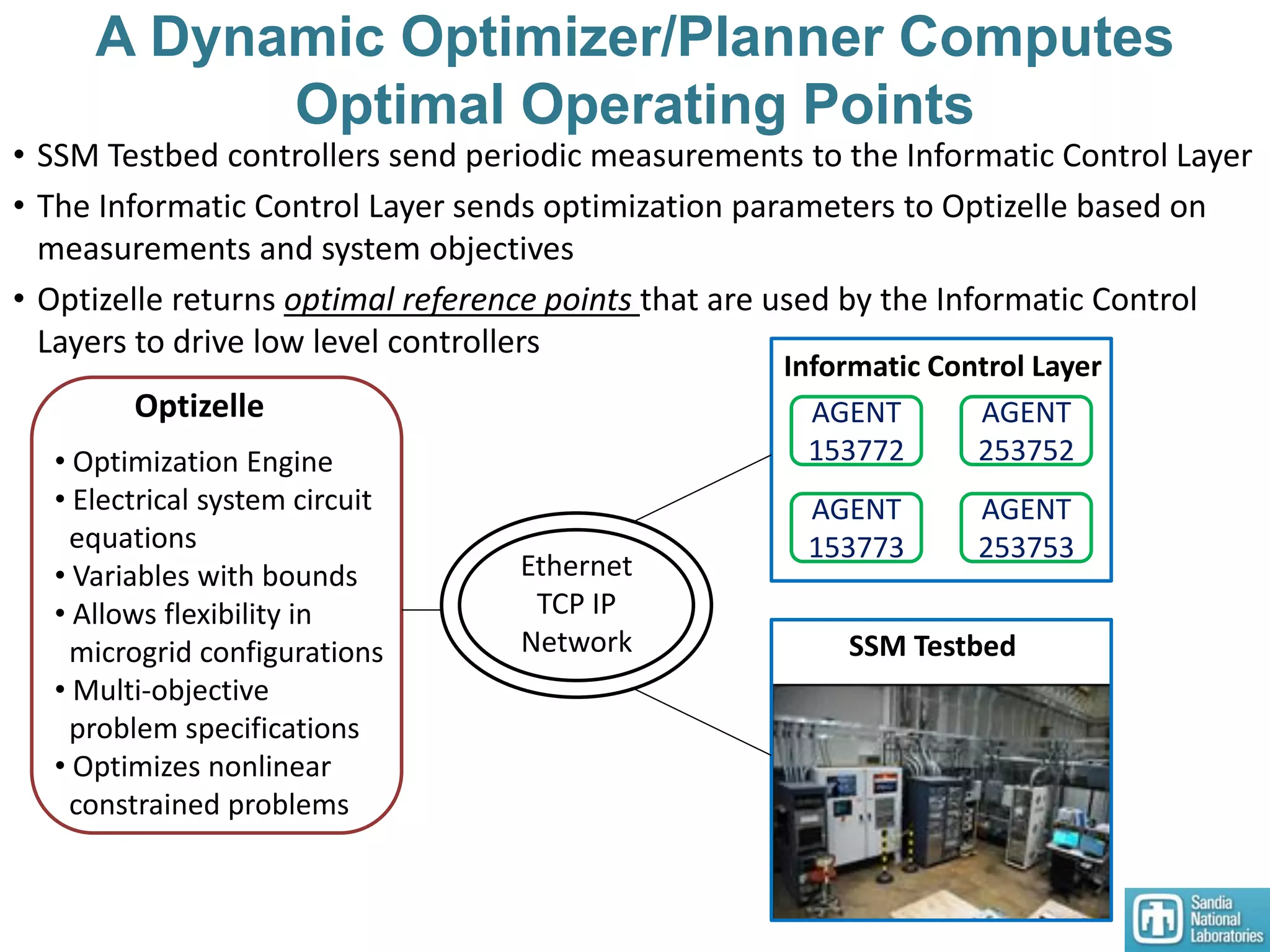
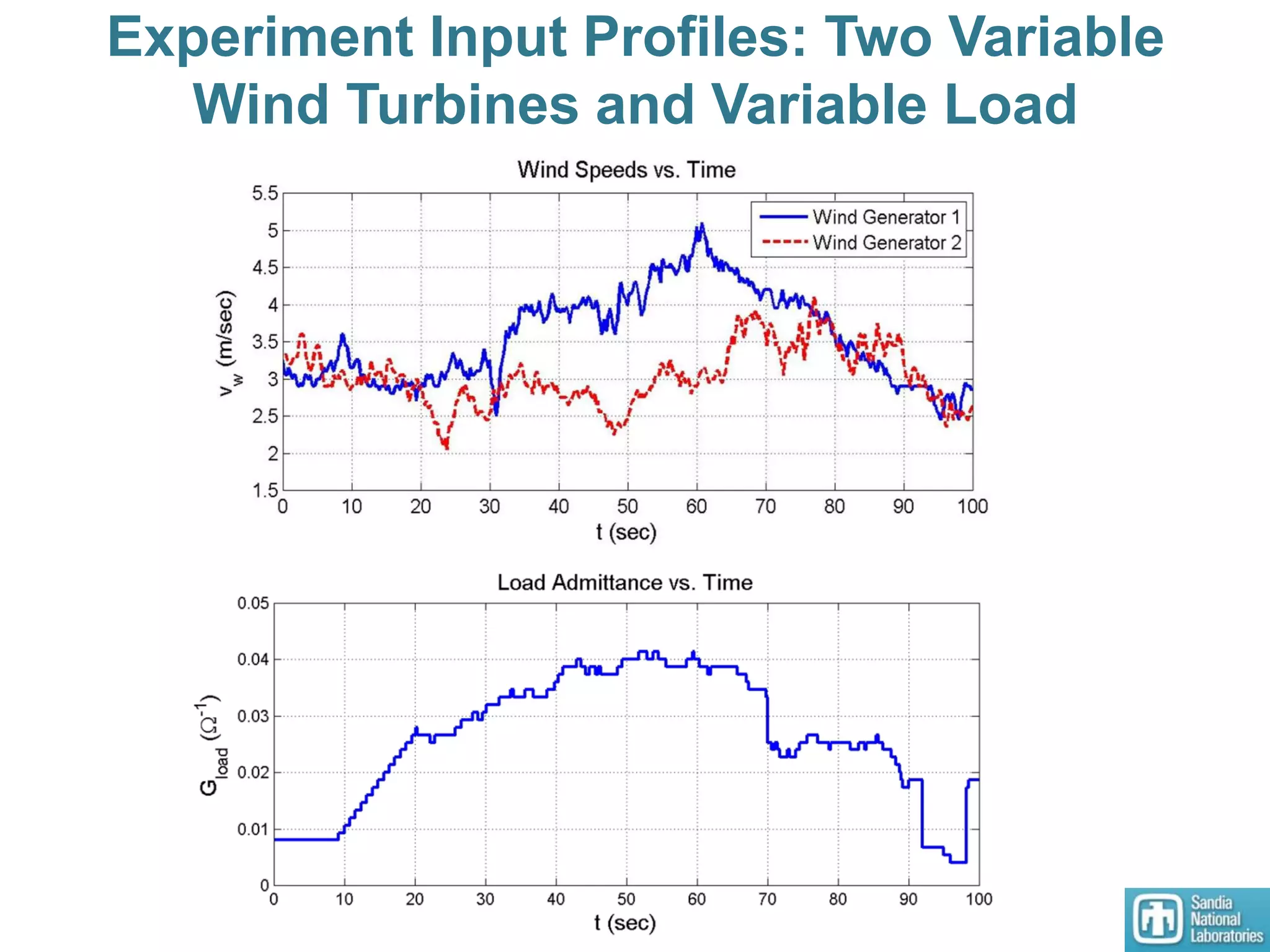
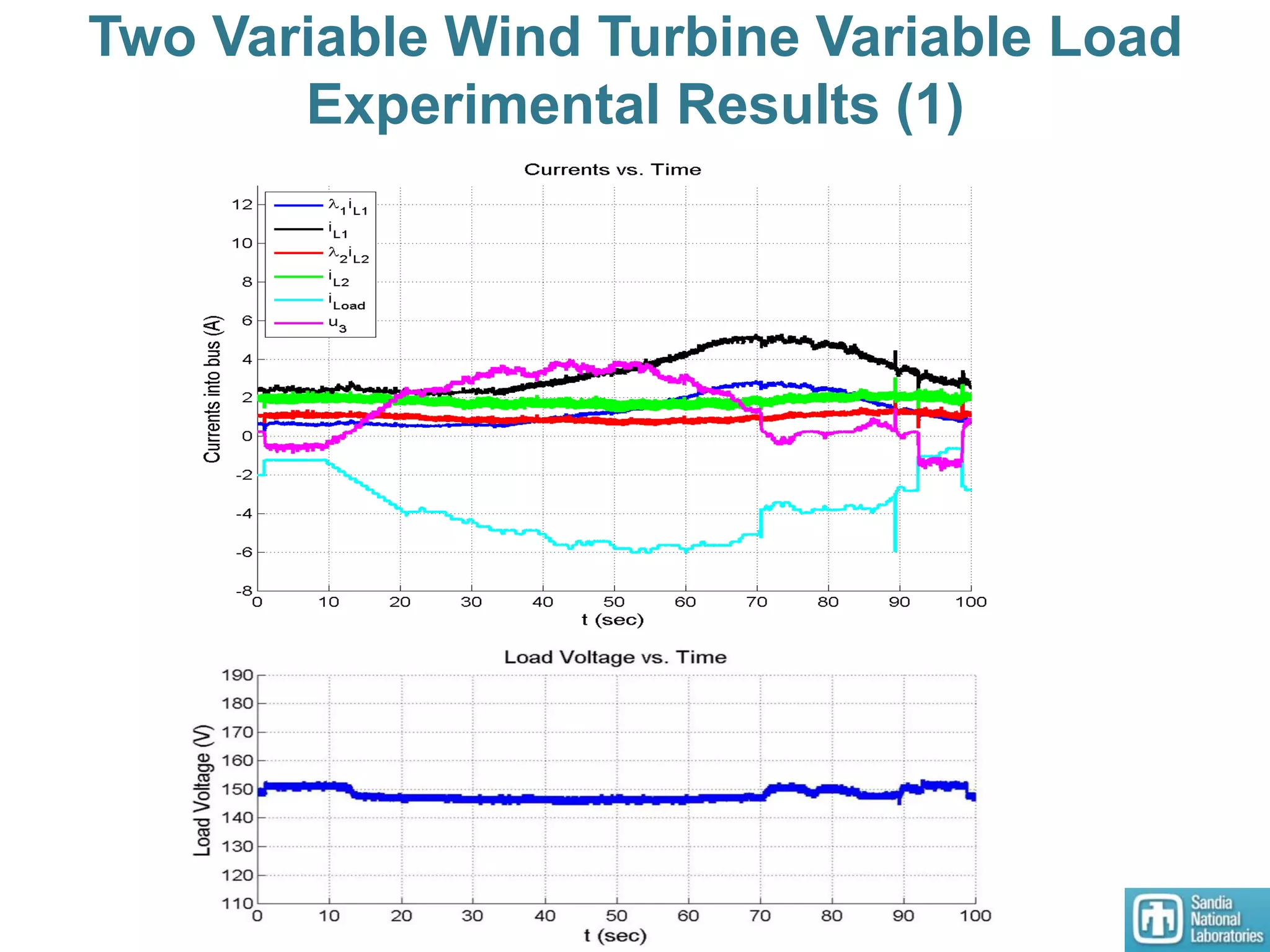
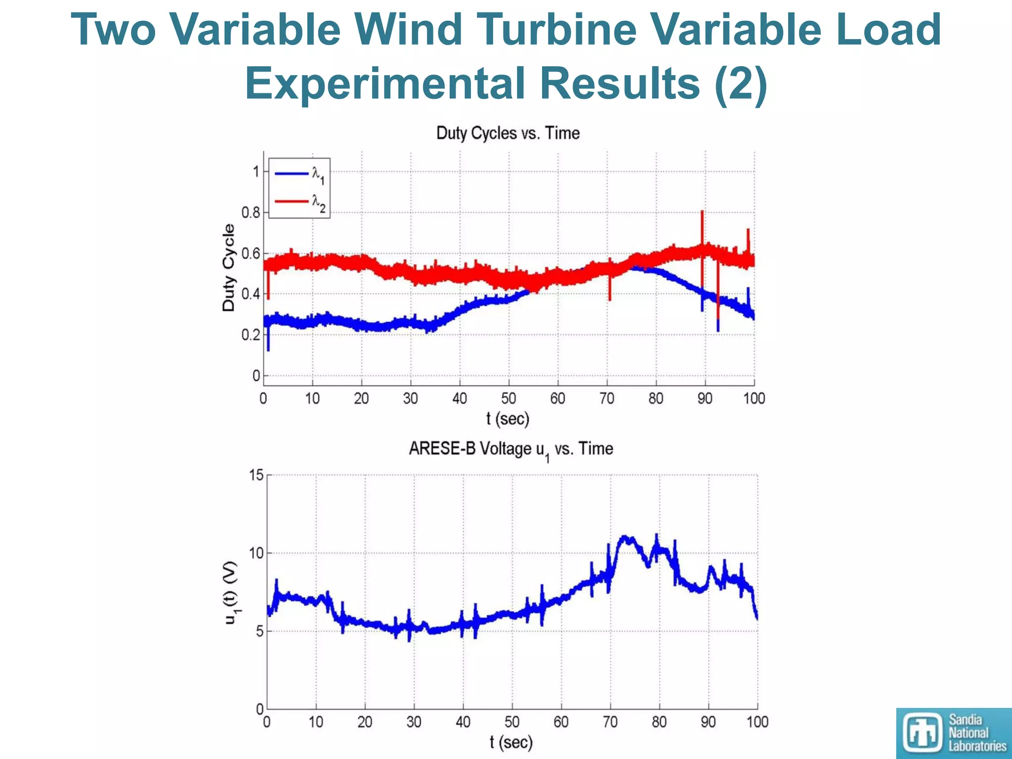
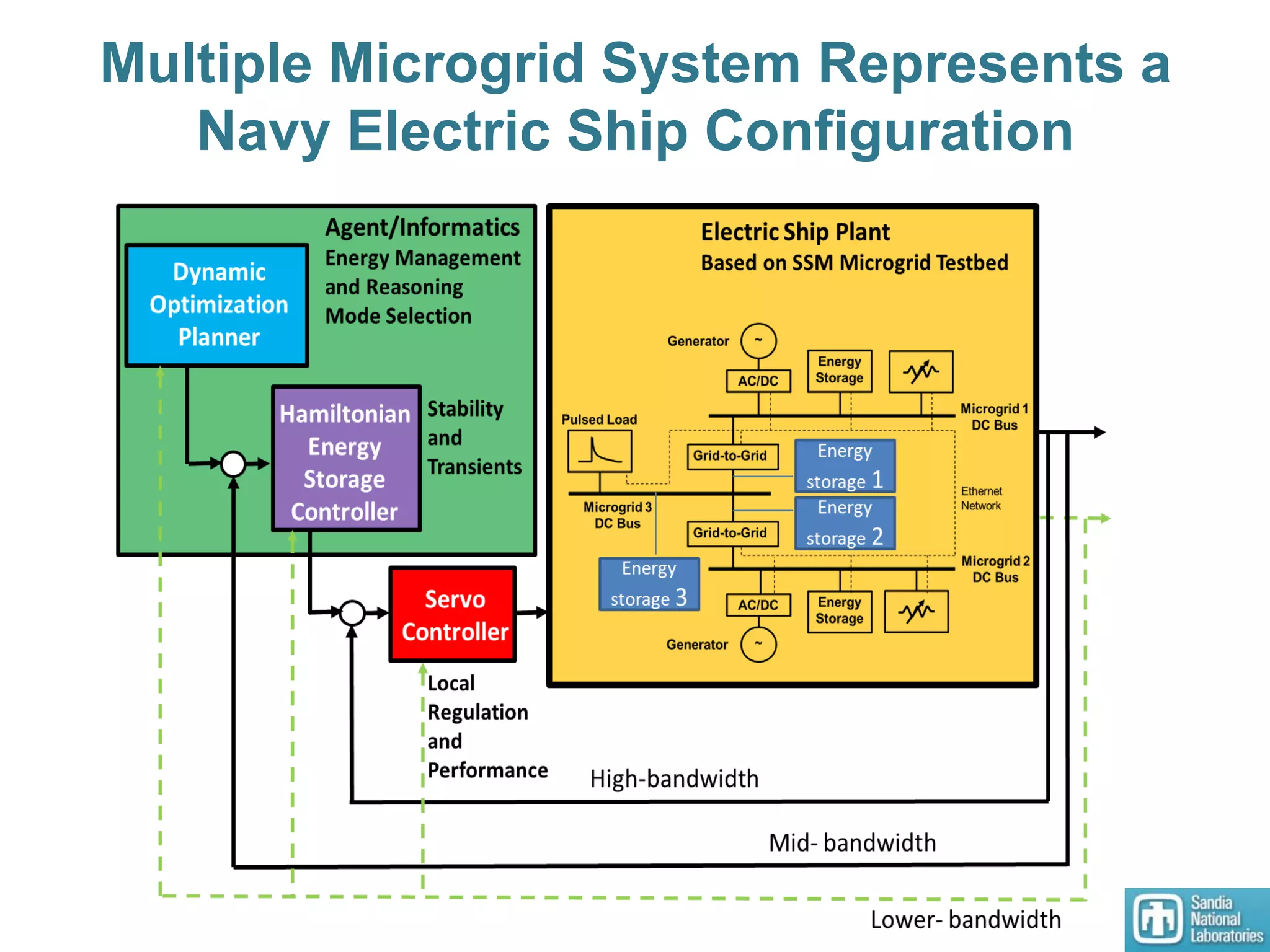
The document summarizes research on designing nonlinear controllers for microgrid systems with stochastic sources and loads. Key points include: 1) A secure scalable microgrid testbed was developed to experimentally test Hamiltonian surface shaping power flow controllers (HSSPFC). 2) Models of single and multiple DC microgrids were formulated to develop optimal operating points using a dynamic optimizer. 3) An HSSPFC nonlinear distributed controller was designed and experimentally validated on a single DC microgrid testbed with variable sources and loads, demonstrating stable voltage regulation.