This document describes 4 laboratories related to radar and remote sensing: 1. Evaluation of SNR and EIRP from the radar range equation for different frequencies and target cross-sections. 2. Calculation of refractive index and obstacle diffraction, including orographic profile download and computation of distance from line of sight. 3. Detection of echo returns through signal integration, including generation of transmitted signals and identification of convolutional signals. 4. Application of radar meteorology, including hourly cumulative rain maps, comparison to terrestrial gauge data, radar accuracy analysis, and spatial averaging of radar data.

1. Radar and Remote Sensing
Laboratories
Ferro Demetrio 207872
Minetto Alex 211419

2. Radar and Remote Sensing Laboratories
Contents
Laboratory 1 - Evaluation of SNR and EIRP from Radar Range Equation 1
Task 1 - SNR Evaluation . . . . . . . . . . . . . . . . . . . . . . . . . . . . . . . . . . . . . . . . . 1
Task 2 - EIRP Evaluation . . . . . . . . . . . . . . . . . . . . . . . . . . . . . . . . . . . . . . . . . 4
Laboratory 2 - Refractive Index and Obstacle Diffraction 7
Task 1 - Orography Acquisition . . . . . . . . . . . . . . . . . . . . . . . . . . . . . . . . . . . . . . 7
Task 2 - Orographic profiles Download . . . . . . . . . . . . . . . . . . . . . . . . . . . . . . . . . . 8
Task 3 - Refractivity Index Computation . . . . . . . . . . . . . . . . . . . . . . . . . . . . . . . . 8
Task 4 - Distance from LOS . . . . . . . . . . . . . . . . . . . . . . . . . . . . . . . . . . . . . . . . 9
Task 5 - Modified Earth Profiles . . . . . . . . . . . . . . . . . . . . . . . . . . . . . . . . . . . . . 9
Task 6 - Modified Earth Distance from LOS . . . . . . . . . . . . . . . . . . . . . . . . . . . . . . . 12
Task 7 - First Fresnel Radius Computation . . . . . . . . . . . . . . . . . . . . . . . . . . . . . . . 14
Laboratory 3 - Detection of echo return by Signal Integration 16
Task 1 - Generation of Transmitted Signal . . . . . . . . . . . . . . . . . . . . . . . . . . . . . . . . 16
Task 2 - Convolutional Signal Identification . . . . . . . . . . . . . . . . . . . . . . . . . . . . . . . 18
Task 3 - Data Integration . . . . . . . . . . . . . . . . . . . . . . . . . . . . . . . . . . . . . . . . . 19
Task 4 - Change of Parameters . . . . . . . . . . . . . . . . . . . . . . . . . . . . . . . . . . . . . . 20
Laboratory 4 - Radar Meteorology Application 22
Task 1 - Hourly Cumulative Rain Map . . . . . . . . . . . . . . . . . . . . . . . . . . . . . . . . . . 22
Task 2 - Hourly Cumulative Behaviour from Terrestrial Gauges . . . . . . . . . . . . . . . . . . . . 23
Task 3 - Radar Accuracy Analysis . . . . . . . . . . . . . . . . . . . . . . . . . . . . . . . . . . . . 24
Task 4 - Spatial Average on Radar Data . . . . . . . . . . . . . . . . . . . . . . . . . . . . . . . . . 25
Ferro Demetrio, Minetto Alex

3. Radar and Remote Sensing Laboratories
Lab 1 - Evaluation of SNR and EIRP from Radar Range Equation
Task 1 - SNR Evaluation
A radar system is characterized by the following parameters: Peak power Pt = 1.5 MW, antenna
gain G = 45 dB, radar losses L = 6 dB, noise figure F = 3 dB, radar bandwidth B = 5 MHz.
The radar minimum and maximum detection ranges are Rmin = 25 Km and Rmax = 165 Km.
Using MATLAB, plot the minimum signal to noise ratio versus detection range in the following
conditions (in two different figures):
1. f0 = 5 GHz and f0 = 10 GHz with σ = 0.1 m2;
2. f0 = 5 GHz assuming three different radar cross section: σ = 0.1 m2, σ = 1 m2, σ = 10 m2;
% Radar Parameters for SNR evaluation from Radar Ranging Equation
2
Rmin=25e3; % Minimum Distance for detection
4 Rmax=165e3; % Maximum Distance for detection
6 % noise is expressed as KbFTB
8 R=Rmin:100:Rmax; % Variable for x-axes to varying distance from radar’s antenna
Pt =1.5e6; % Transmitting Power
10 G=10ˆ(45/10); % Transmitting antenna Gain
L=10ˆ(6/10); % System Loss
12 F=10ˆ(3/10); % Noise Figure
B=5e6; % Bandwidth of pulse
14 Kb=1.38e-23; % Boltzman Constant
16 % Case 1
18 c=299792458; % Speed of Light
freq = 5e9; % Frequency of transmission [first]
20 freq2= 10e9; % Frequency of transmission [second]
lambda = c/freq;
22 lambda2= c/freq2;
24 s=0.1; % Target cross section
n=1; % Number of pulses
26 T0=16+273; % Kelvin Temperature of system
From the radar ranging equation for the computation of received power we can evaluate SNR as
follows:
Pr =
PtG2λ2σn
(4π)3R4Ls
(1)
Pn = KbFTB (2)
SNR =
Pr
Pn
=
Pr
KbFTB
=
PtG2λ2σn
(4π)3R4LsKbFTB
(3)
Ferro Demetrio, Minetto Alex Page 1 of 27

4. Radar and Remote Sensing Laboratories
We reported the formulas in MATLAB and then plotted the behaviour of SNR with respect to the
distance between radar and target.
% Double SNR evaluation for f1 and f2
2
SNR=(Pt*Gˆ2*lambdaˆ2*s*n)./(((4*pi)ˆ3)*(Kb*T0*B*F)*L*(R.ˆ4));
4 SNR2=(Pt*Gˆ2*lambda2ˆ2*s*n)./(((4*pi)ˆ3)*(Kb*T0*B*F)*L*(R.ˆ4));
6 figure(’Name’,’SNR related to distance’);
plot(R,10*log10(SNR),’b’,R,10*log10(SNR2),’r’)
8 hold on;
grid on;
10 title(’SNR of Radar’);
ylabel(’SNR’)
12 xlabel(’Distance R’)
legend(’frequency = 5 Ghz’,’frequency = 10 Ghz’);
As we expected the value of SNR decreases along the distance, basically because free space attenu-
ation degrades the output signal proportionally to the fourth power of distance R. This is a simple
simulation which shows how geometrical distance can affect propagation phenomena, any other
kind of attenuation is not taken in account except for the system loss that is moreover constant
along the link because is a proper property of the system.
Distance R ×10 5
0.2 0.4 0.6 0.8 1 1.2 1.4 1.6 1.8
SNR
-5
0
5
10
15
20
25
30
35
40
SNR of Radar
frequency = 5 Ghz
frequency = 10 Ghz
As we can notice in the plot reported above, higher frequencies suffer noise in a stronger way re-
spect with the lower ones. This is immediate from the equation point of view because frequency
is invertially proportional to λ, so, if we adopt an higher frequency we reduce the wavelength and
the respective SNR value.
The second part of the exercise proposes us to evaluate the same quantity for three different cross
section values. We simply report the MATLAB code that is almost the same as before. We have
to precise that cross section σ is a quantity that represents the capacity of target to reflect the
incoming signal, it is linked to the surface and to the volume of the object but does not represent
Ferro Demetrio, Minetto Alex Page 2 of 27

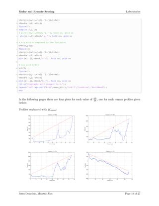
5. Radar and Remote Sensing Laboratories
strictly this geometrical feature.
sig1=[0.1 1 10]; % Vector of different cross sections
2 color=[1 0 0.5 1 0.5];
4 figure(’Name’,’SNR with different Cross Section’);
for i=1:3
6 SNR=(Pt*Gˆ2*lambdaˆ2*sig1(i)*n)./(((4*pi)ˆ3)*Kb*T0*B*F*L*(R.ˆ4));
plot(R,10*log10(SNR),’color’,[color(i+1),color(i+2),color(i)])
8 grid on;
hold on;
10 end
title(’SNR of Radar with different cross section’);
12 ylabel(’SNR’)
xlabel(’Distance R’)
14 legend(’cross sec. = 0.1 mˆ2’,’cross sec. = 1 mˆ2’,’cross sec. = 10 mˆ2’);
Distance R ×10 5
0.2 0.4 0.6 0.8 1 1.2 1.4 1.6 1.8
SNR
0
10
20
30
40
50
60
SNR of Radar with different cross section
cross sec. = 0.1 m
2
cross sec. = 1 m
2
cross sec. = 10 m 2
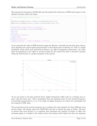
As we can see in the plot, radar cross section that is in some way the ”equivalent reflective surface”
of the target, has a strong impact on the SNR evaluation, signals that meet target with bigger cross
section are less sensitive with respect to the noise power.
For the target with the smallest cross-section, the SNR falls under 10 dB, so it could be more
difficult to individuate original transmitted pulse without some other solution to make it stronger
than the noise (like for example data integration or some modulation methods). Even in this
simulation, equations confirm our data behaviour, received power Pr is proportional to the target
cross section, it is the effective equivalent area that reaches the power density emitted by radar’s
antenna.
Ferro Demetrio, Minetto Alex Page 3 of 27

6. Radar and Remote Sensing Laboratories
Task 2 - EIRP Evaluation
A surveillance radar is characterized by the following parameters: minimum SNR = 15 dB, radar
losses L = 6dB and noise figure F = 3 dB. The radar scan time is Tsc = 2.5 s. The solid angle
extent of the atmospheric volume to be surveilled is Θ = 3 srad.
The minimum and maximum detection ranges are Rmin = 25 Km and Rmax = 165 Km.
Using MATLAB plot the EIRP versus detection range in the following conditions:
1. f0 = 5 GHz and f0 = 10 GHz with σ = 0.1 m2;
2. f0 = 5 GHz assuming three different radar cross section: σ = 0.1 m2, σ = 1 m2, σ = 10 m2;
Remembering that EIRP (Equivalent Isotropic Radiated Power) is defined as the product Pavg · G
where Pavg is the averaged power characterizing the transmitted waveform (pulsed waveform with
pulse length τ and Pulse Repetition Interval Ti) and G is the radar antenna gain which, in turn,
can be defined in terms of the antennas half power beam-widths θ3dB and φ3dB, as it follows using
Top-Hat Approximation:
G =
4π
θ3dB · φ3dB
(4)
For the radar’s characterization, we use almost the same code as before. In order to implement
the same expression of radar equation we have to convert quantities expressed in dB in linear values.
%% Radar Specifics for SNR evaluation
2
Rmin=25e3; %Minimum Distance for detection
4 Rmax=165e3; %Maximum Distance for detection
6 % noise is expressed as KbFTB
8 R=Rmin:100:Rmax; %Variable for x-axes to varying distance from radar
Pt =1.5e6; %Transmission Power
10 G=10ˆ(45/10); %Transmitting antenna Gain
L=10ˆ(6/10); %System Loss
12 F=10ˆ(3/10); %Noise Figure
B=5e6; %Bandwidth of pulse
14 Kb=1.38e-23; %Boltzman Costant
16 %%case one
c=299792458; %Speed of Light
18 freq = 5e9; %Frequency of transmission [first]
freq2= 10e9; %Frequency of transmission [second]
20 lambda = c/freq;
lambda2= c/freq2;
22
s=0.1; %Target cross section
24 n=1; %number of pulses
T0=16+273; %Kelvin Temperature of system
Ferro Demetrio, Minetto Alex Page 4 of 27

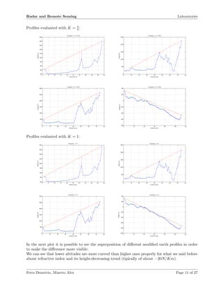
7. Radar and Remote Sensing Laboratories
By using theoretical hints we substitute G of radar ranging equation with the proper one evaluated
in relation of beam-width solid angle. Inverting SNR equation we can solve the problem specification
of maximum SNR.
EIRP = Pavg · G =
Pt4π
Tsσ
(5)
Pt =
(4π)3R4LsKbFTB · (SNR)
G2λ2σn
(6)
EIRP =
(4π)3R4LsKbFTB · (SNR) · 4π
(4π/Ω)2λ2σn
=
(4π)2R4LsKbFTB · (SNR) · Ω
G2λ2σnTs
(7)
We can implement this derivation in MATLAB and then we evaluate the behaviour of EIRP in
relation to distance from the target.
EIRP=(((4*pi)ˆ2)*Kb*T0*F*L*(R.ˆ4)*omega*SNR)./((lambdaˆ2)*s*n*Tscan); % Linear format NO dB
2 EIRP2=(((4*pi)ˆ2)*Kb*T0*F*L*(R.ˆ4)*omega*SNR)./((lambda2ˆ2)*s*n*Tscan);
4 plot(R,10*log10(EIRP),R,10*log10(EIRP2),’r’); %Plot in dB form
grid on;
6 title(’EIRP of Radar with different frequencies’);
ylabel(’EIRP [dB]’)
8 xlabel(’Distance [Km]’)
legend(’frequency = 5 GHz’,’frequency = 10 GHz’,’Location’,’SouthEast’);
Distance [Km] ×10 5
0.2 0.4 0.6 0.8 1 1.2 1.4 1.6 1.8
EIRP[dB]
40
45
50
55
60
65
70
75
80
85
EIRP of Radar with different frequencies
frequency = 5 GHz
frequency = 10 GHz
We can proceed evaluating the distribution of EIRP function related with target cross section.
Data are the same as the first exercise and so we can keep a similar code that is reported below for
completion.
Ferro Demetrio, Minetto Alex Page 5 of 27

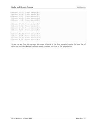
8. Radar and Remote Sensing Laboratories
%% Subplot for different cross section case two
2
sig1=[0.1 1 10];
4 color=[1 0 0.5 1 0.5];
6 figure();
for i=1:3
8 EIRP=(((4*pi)ˆ2)*Kb*T0*F*L*(R.ˆ4)*omega*SNR)./((lambdaˆ2)*sig1(i)*n*Tscan);
plot(R,10*log10(EIRP),’color’,[color(i+1),color(i+2),color(i)])
10 grid on;
hold on;
12 end
title(’EIRP of Radar with different cross section’);
14 ylabel(’EIRP [dB]’)
xlabel(’Distance [Km]’)
16 legend(’cross sec. = 0.1 mˆ2’,’cross sec. = 1 mˆ2’,’cross sec. = 10 mˆ2’,’Location’,’SouthEast
’);
Here it is reported the ouput plot of the previous code section. We can notice that the behaviour
of EIRP with respect to SNR is exactly inverse, that shows us the correct inverse proportionality
between the two quantities.
Distance [Km] ×10 5
0.2 0.4 0.6 0.8 1 1.2 1.4 1.6 1.8
EIRP[dB]
20
30
40
50
60
70
80
EIRP of Radar with different cross section
cross sec. = 0.1 m
2
cross sec. = 1 m 2
cross sec. = 10 m
2
Since smaller object reflect usually a reduced amount of power, EIRP value has to be higher in
order to keep constant the SNR with low value of Cross Scattering Section.
Ferro Demetrio, Minetto Alex Page 6 of 27

9. Radar and Remote Sensing Laboratories
Laboratory 2 - Refractive Index and Obstacle Diffraction
Evaluate the possibility to create a communication link between the two extreme points.
1. Download from the personal web page one of the ASCII files containing the terrain profile
(profx.jpf where x=1, · · · , 4) and plot it. These profiles are extracted from the Piedmont
Numerical Terrain Modelling.
2. Download a radiosounding profile (from Cuneo-Levaldigi if available or Milano-Linate site).
3. Compute the spatial-averaged K value using the refractivity gradient evaluated from ra-
diosounding data in the height layers defined by the orographic profile, (Re = Earths radius
= 6378 Km)
4. Evaluate the distance of the worst obstacle from the line of sight, considering a refractivity
gradient dN/dh = -157 N/km
5. Plot the orographic profile above the modified Earth, taking into account also the two following
cases:
(a) a value K = 4/3
(b) the averaged Kmean value evaluated using radiosounding
6. Evaluate the distance of the worst obstacle from the line of sight considering 5a and 5b cases.
7. Compare these distances with the first Fresnel radius dimension (at the point where the worst
obstacle is), considering a working frequency of 10 GHz and evaluate the attenuation due to
diffraction effects, considering the three cases (dN/dh = -157 N/km, 5a case, 5b case).
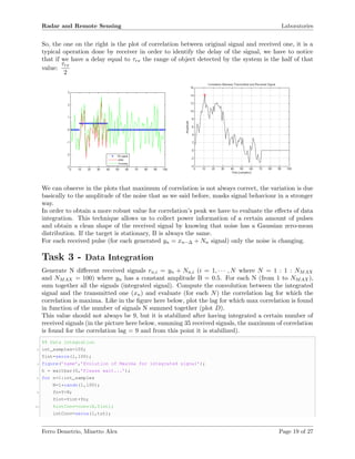
Task 1 - Orography Acquisition
We are just commenting the first two tasks in order to show the MATLAB’s code for the data
processing and the relative plots. We report below the plots of terrain profiles from Piedmont
model.
for i=1:4
2 x=load(strcat(’prof’,int2str(i),’.ipf’)); % data loading from profx.ipf files
figure(1)
4 subplot(2,2,i)
%plot(x), hold on
6 plot(x(:,1),x(:,2),’-b.’), grid on
title(strcat(’Orography ’,int2str(i)));
8 xlabel(’Distance [km]’);
ylabel(’Height [m]’);
10 end
The code before is useful to get geographic profiles from proper files and plot them in order to see
the orographic element’s shape.
Ferro Demetrio, Minetto Alex Page 7 of 27

10. Radar and Remote Sensing Laboratories
Distance [km]
0 10 20 30 40 50
Height[m]
200
400
600
800
1000
1200
1400
1600
1800
2000
prof1.ipf
Distance [km]
0 20 40 60 80
Height[m]
0
500
1000
1500
2000
2500
3000
prof2.ipf
Distance [km]
0 20 40 60 80
Height[m]
0
500
1000
1500
2000
2500
3000
prof3.ipf
Distance [km]
0 20 40 60 80 100
Height[m]
0
100
200
300
400
500
prof4.ipf
Task 2 - Orographic profiles Download
Downloading Radiosound profile for empirical evaluation of refractive index, we have to extract
specific information useful for the Beam and Dutton Formulae. As we can see in the extract of
code we need the atmospheric pressure, relative altitude, temperature and relative humidity, so we
extract this informations from the downloaded file.
Task 3 - Refractivity Index Computation
And then we compute the atmospheric refractivity by using Beem and Dutton Formulae. Through
the following cycle we evaluate the Kmean for each terrain profile loaded before. Kmean represents
an approximation of the gradient of refractive index n with respect to the altitude, once converted
in N units, it will be a multiplicative coefficient useful to modify earth’s radius in our simulation
model.
%% Points 2-3
2
mRSP=load(’cuneo-levaldigi.txt’);
4
vHPA=mRSP(:,1); % Atmospheric Pressure
6 vHGT=mRSP(:,2); % Height
vTEMP=mRSP(:,3); % Temperature
8 vRELH=mRSP(:,5); % Relative Humidity
vWVPP=(vRELH/100*6.122).*(exp((17.67*vTEMP)./(243.5+vTEMP)));
10 % Water Vapour partial pressure e(h)
12 % Atmoshperic Refractivity N(h) with Been and Dutton Formulae
N=77.6*(vHPA./(vTEMP+273.15))-6*(vWVPP./(vTEMP+273.15))+3.73e5*(vWVPP./(vTEMP+273.15).ˆ2);
14
Re=6378e3; % Earth’s radius
16 dNoverdH=0; % Gradient variable for following calculations
mean_k=zeros(1,4); % Vector of k coefficients
18
for j=1:4
20 % Interval where to compute kmean
[vIndStart,nValue1]=find(vHGT > nTxHeight(j));
22 [vIndStop,nValue2]=find(vHGT > nRxHeight(j));
Nlev=vIndStart(1):vIndStop(end)-1;
24
for i=Nlev
26 dNoverdH=dNoverdH+(N(i+1)-N(i))/(vHGT(i+1)-vHGT(i))/length(Nlev);
end
Ferro Demetrio, Minetto Alex Page 8 of 27

11. Radar and Remote Sensing Laboratories
28
mean_k(j)=1/(1+(Re*1e-6*dNoverdH));
30
fprintf(’The mean dN/dH of k-order is: %2.2dn’,mean_k(j));
32 end
The output of this extract of code is the following:
The mean dN/dH of k-order is: 1.07e+00
2 The mean dN/dH of k-order is: 1.14e+00
The mean dN/dH of k-order is: 1.23e+00
4 The mean dN/dH of k-order is: 1.33e+00
As we can notice in the output lines, the mean value of the refractive index gradient decrease with
the altitude. Lower values refer to lower profiles scenario while Kmean = 1.33, which represent
a quite strong modification of earth’s curvature, is relative to near-sea-level profile. This is a
typical trend for the refractive index due to the variations in temperature and humidity through
the atmosphere that usually decreases with the height.
Task 4 - Distance from LOS
Evaluating distances (or better height) considering a refractivity gradient dN/dh = −157N/Km
means to consider the propagation bending with a curvature that is exactly the same of the earth’s
surface (practically we don’t have any modifications on the line of sight height), so it’s the same
issue to compute this amount considering Kmean = 1 .
So we can evaluate the behaviour of bending with the variation of K as it is request at point 6.
We report here the portion of code used to evaluate the 4th point of this assignment, the output
of the code is instead reported below in task 6.
% Refractivity index
2 dNdH=-157;
%ourK=1/(1+Re*1e-6*dNdH);
4 %mean_k=1;
x=load(strcat(’prof’,int2str(j),’.ipf’));
6 [AbsLOS(:,1), nDifferencePrec(:,1)]=Distance_from_obstacle_to_LOS(ourK,1);
Task 5 - Modified Earth Profiles
We need to plot the terrain profiles with the proper bending induced by refractive index. This is a
useful representation that allows us to keep the propagation line horizontal and change curvature
of the ground in order to appreciate the real distance of obstacles from line of sight. We have to
compute the variation in height for each point of the profile and then we can modify the original
orography with the modified earth radius approach.
%% Point 5
2 for i=1:4
x=load(strcat(’prof’,int2str(i),’.ipf’));
4
% try with k=1
6 k=1e0;
Ferro Demetrio, Minetto Alex Page 9 of 27

12. Radar and Remote Sensing Laboratories
vVarh=(x(:,1).*1e3).ˆ2./(2*k*Re);
8 vHmod=x(:,2)-vVarh;
figure(2)
10 subplot(2,2,i);
% plot(x(:,1),vHmod,’g.-’), hold on, grid on
12 plot(x(:,1),vHmod,’g.-’), hold on, grid on
14 % try with k computed in the 3rd point
k=mean_k(i);
16 figure(2)
vVarh=(x(:,1).*1e3).ˆ2./(2*k*Re);
18 vHmod=x(:,2)-vVarh;
plot(x(:,1),vHmod,’r.-’), hold on, grid on
20
% now with k=4/3
22 k=4/3;
figure(2)
24 vVarh=(x(:,1).*1e3).ˆ2./(2*k*Re);
vHmod=x(:,2)-vVarh;
26 plot(x(:,1),vHmod,’b.-’), hold on, grid on
title(’Orography with respect to k.’);
28 legend(’k=1’,sprintf(’k=%d’,mean_k(i)),’k=4/3’,’Location’,’NorthWest’);
end
In the following pages there are four plots for each value of dN
dh , one for each terrain profiles given
before.
Profiles evaluated with Kmean:
Ferro Demetrio, Minetto Alex Page 10 of 27

13. Radar and Remote Sensing Laboratories
Profiles evaluated with K = 4
3:
Profiles evaluated with K = 1:
In the next plot it is possible to see the superposition of different modified earth profiles in order
to make the difference more visible.
We can see that lower altitudes are more curved than higher ones properly for what we said before
about refractive index and its height-decreasing trend (tipically of about −20N/Km).
Ferro Demetrio, Minetto Alex Page 11 of 27

14. Radar and Remote Sensing Laboratories
Distance [Km]
0 10 20 30 40 50
Height[m]
0
500
1000
1500
2000
Orography with respect to k.
k=1
k=1.665479e+00
k=4/3
Distance [Km]
0 10 20 30 40 50 60 70 80
Height[m]
0
500
1000
1500
2000
2500
Orography with respect to k.
k=1
k=1.204258e+00
k=4/3
Distance [Km]
0 10 20 30 40 50 60 70 80
Height[m]
0
500
1000
1500
2000
2500
3000
Orography with respect to k.
k=1
k=1.204258e+00
k=4/3
Distance [Km]
0 20 40 60 80 100 120
Height[m]
-1000
-800
-600
-400
-200
0
200
400
Orography with respect to k.
k=1
k=1.174782e+00
k=4/3
Task 6 - Modified Earth Distance from LOS
Proceeding from Task 4, we evaluate the distance of the worst obstacles from the lines of sight of
each transreceiving system. Here is reported the full matlab code for the accumulation in a vector
of various data collected about this point.
For this Task we have developed a function that evaluates the specific distance of obstacles from
line of sight. The code of the function is reported after the code’s lines of computation. The
function accepts as parameters the index of reference figure (relative to ground’s profile) and the
Kmean coefficient for earth’s curvature.
%% Point 6 evaluate the distance of the worst obstacla from the LOS
2 [AbsLOS(:,2), nDifferencePrec(:,2)]=Distance_from_obstacle_to_LOS(1,3);
[AbsLOS(:,3), nDifferencePrec(:,3)]=Distance_from_obstacle_to_LOS(mean_k,4);
4 [AbsLOS(:,4), nDifferencePrec(:,4)]=Distance_from_obstacle_to_LOS(4/3,5);
6 %% Code for Distance_from_obstacle_to_LOS(n,m)
function [AbsLOS, nDifferencePrec]=Distance_from_obstacle_to_LOS(k,indfigure)
8 Re=6378e3;
AbsLOS=zeros(1,4);
10 nDifferencePrec=zeros(1,4)+1e10;
12 for ii=1:4
14 x=load(strcat(’prof’,int2str(ii),’.ipf’));
16 if(length(k)>1)
Ferro Demetrio, Minetto Alex Page 12 of 27

15. Radar and Remote Sensing Laboratories
vk=k(ii);
18 vVarh=(x(:,1).*1e3).ˆ2./(2*vk*Re);
x(:,2)=x(:,2)-vVarh;
20 elseif(k==0)
vk=k;
22 else
vk=k;
24 vVarh=(x(:,1).*1e3).ˆ2./(2*vk*Re);
x(:,2)=x(:,2)-vVarh;
26 end
28 % Compute LOS
nDTx=x(1,1)*1e3;
30 nDRx=x(end,1)*1e3-nDTx;
nHTx=x(1,2);
32 nHRx=x(end,2);
vHighLOS=linspace(nHTx, nHRx, length(x(:,1)));
34 AbsLOS(ii)=sqrt((nDRx)ˆ2+(nHTx-nHRx)ˆ2);
36
% Find Possible Peaks
38 [vPeaks,vIndexPeaks]=findpeaks(x(:,2));
vDifference=vHighLOS-x(:,2)’;
40
% Find Highest Obstacle
42 nIndPeaks=1;
nIndObst=1;
44
for nInd=2:length(vDifference)-1
46 if nIndPeaks<=length(vIndexPeaks)
if(nInd==vIndexPeaks(nIndPeaks))
48 if(vDifference(nInd)<nDifferencePrec(ii))
nDifferencePrec(ii)=vDifference(nInd);
50 nIndObst=nInd;
end
52 nIndPeaks=nIndPeaks+1;
end
54 end
end
56
% Plot profile
58 figure(indfigure)
subplot(2,2,ii)
60 plot(x(:,1),x(:,2),’-b.’); hold on, grid on
62 % Plot LOS
plot(x(:,1),vHighLOS,’r’); hold on
64
% Plot Peaks
66 for j=1:length(vIndexPeaks)
plot(x(vIndexPeaks(j),1),x(vIndexPeaks(j),2),’g*’);
68 end
Ferro Demetrio, Minetto Alex Page 13 of 27

16. Radar and Remote Sensing Laboratories
70 % Plot Highest Peaks
for kk=1:length(nIndObst)
72 plot(x(nIndObst(kk),1),x(nIndObst(kk),2),’mO’); hold on
plot([x(nIndObst(kk),1) x(nIndObst(kk),1)],[x(nIndObst(kk),2) nDifferencePrec(ii)+x(nIndObst(
kk),2)],’m’), hold on
74 plot([x(nIndObst(kk),1) x(nIndObst(kk),1)],[x(nIndObst(kk),2) nDifferencePrec(ii)+x(nIndObst(
kk),2)],’m’), hold on
end
76
% Titles
78 %if(k>0)
title([’Orography ’ num2str(ii) ’, k=’ num2str(vk)])
80 %else
%title([’Orography ’ num2str(ii)])
82 %end
xlabel(’Distance [km]’);
84 ylabel(’Height [m]’);
end
86 end
This implementation provides also plots of LOS over several modified terrain profiles and in the
overlying plot, it points out the highest peaks of each profile. In order to avoid a very long report,
plots are reported in the previous task as superposition of different requested figures.
Task 7 - First Fresnel Radius Computation
The following code implements the computation of First Fresnel Radius for the different profiles:
%% Point 7 compute the first fresnel radius
2
freq=1e10;
4 c0=physconst(’LightSpeed’);
lambda=c0/freq;
6
Rf=zeros(1,4);
8
for i=1:size(nDifferencePrec,2)
10 for j=1:size(nDifferencePrec,1)
Rf=sqrt(lambda*AbsLOS./4);
12 fprintf(’Distance: %3.2f tFresnel radius:%3.2fn’,nDifferencePrec(j,i),Rf(j,i));
end
14 fprintf(’n’);
end
We report below the final outuput which include the distance of the worst obstacle for each orogra-
phy and the respective fresnel radius in order to evaluate immediately how much the obstacle can
degrade propagation performance.
Distance: 432.97 Fresnel radius:18.76
2 Distance: 87.10 Fresnel radius:23.49
Distance: 248.65 Fresnel radius:23.48
Ferro Demetrio, Minetto Alex Page 14 of 27

17. Radar and Remote Sensing Laboratories
4 Distance: 193.32 Fresnel radius:28.81
Distance: 393.61 Fresnel radius:18.76
6 Distance: 19.02 Fresnel radius:23.49
Distance: 153.81 Fresnel radius:23.48
8 Distance: -20.42 Fresnel radius:28.81
10 Distance: 396.02 Fresnel radius:18.76
Distance: 31.36 Fresnel radius:23.49
12 Distance: 171.26 Fresnel radius:23.48
Distance: 30.36 Fresnel radius:28.81
14
Distance: 403.45 Fresnel radius:18.76
16 Distance: 44.19 Fresnel radius:23.49
Distance: 177.52 Fresnel radius:23.48
18 Distance: 31.45 Fresnel radius:28.81
As we can see from the outputs, the worst obstacle in the first scenario is quite far from line of
sight and since the Fresnel radius is small it cannot interfere in the propagation.
Ferro Demetrio, Minetto Alex Page 15 of 27

18. Radar and Remote Sensing Laboratories
Laboratory 3 - Detection of echo return by Signal Integration
Task 1 - Generation of Transmitted Signal
The transmitted signal xn is a rectangular pulse with amplitude A and fixed length τ. Generate
the transmitted signal in Matlab for A = 1 and τ = 30 (samples). The total length of the signal is
100 samples. Plot it.
% Transmitted signal
2 A=1;
t=30;
4 tot=100;
X=[A*ones(1,t) zeros(1,tot-t)];
6 figure(’name’,’Transmitted Signal’);
plot(X,’--’,’linewidth’,3)
8 grid on;
axis([0 100 0 1.2])
10
%% Received Signal
12 B=0.5;
tr=30;
14 delay=9;
N=randn(1,100);
16
Y=[zeros(1,delay) B*ones(1,tr) zeros(1,tot-delay-tr)];
18 figure(’name’,’Received Theoretical Signal’);
plot(Y,’--r’,’linewidth’,3)
20 title(’Ideal Received Signal’)
xlabel(’Time [samples]’)
22 ylabel(’Amplitude’)
grid on;
24 axis([0 100 0 1.2]);
Time [samples]
0 10 20 30 40 50 60 70 80 90 100
Amplitude
0
0.2
0.4
0.6
0.8
1
1.2
Transmitted Signal
Time [samples]
0 10 20 30 40 50 60 70 80 90 100
Amplitude
0
0.2
0.4
0.6
0.8
1
1.2
Ideal received Signal
We plot both the ideal TX and RX signals in order to evaluate easily what are the shape modifica-
tions due to noise in the second part of this exercise. For the ideal RX signal we have just applied
an attenuation of amplitude that could be modelled as a typical free space loss.
The signal received yn is a rectangular pulse with amplitude B = 0.5, length τ = 30 samples, delay
of ∆ = 9 samples, plus additional noise. Noise signal amplitude Nn should be modeled as Gaussian
Ferro Demetrio, Minetto Alex Page 16 of 27

19. Radar and Remote Sensing Laboratories
distributed random variable with zero mean and a unitary standard deviation.
Check that the noise is correctly generated plotting an histogram showing the distribution of noise
samples. Generate the overall received signal (the total length of the signal is 100 samples). Plot
all together the transmitted signal (xn), the noise (Nn) and the received signal (yn = xn−∆ + Nn).
figure(’name’,’Received Noisy Signal’);
2 plot(Y,’k--’,’linewidth’,2)
hold on
4 title(’Noise vs Ideal Received Signal’)
xlabel(’Time [samples]’)
6 ylabel(’Amplitude’)
plot(N,’r’,’linewidth’,1)
-4 -3 -2 -1 0 1 2 3
0
5
10
15
20
25
30
Simulated Noise Distribution
0 10 20 30 40 50 60 70 80 90 100
-3
-2
-1
0
1
2
3
Additive White Gaussian Noise Samples
Thanks to the plots we can notice that noise amplitude is considerably higher than signal amplitude.
At the receiver, original signal is completely hide by the noise and it seems to be unreachable. On
the right we have verified noise’s samples distribution which appears exactly Gaussian.
0 10 20 30 40 50 60 70 80 90 100
-3
-2
-1
0
1
2
3
RX signal
WGN
Yn+noise
Ferro Demetrio, Minetto Alex Page 17 of 27

20. Radar and Remote Sensing Laboratories
As requested, the following plot shows a superposition of the different elements in signal transmis-
sion. We have to underline that the plot does not correspond to the same previous realizations
because it is the product of a new random instance of WGN.
Task 6 - Convolutional Signal Identification
Generate the Matlab code for evaluating the convolution between the received signal (yn = xn−∆ +
Nn) and the transmitted one (xn). Plot the entire convolution (Cn(x, y)) and identify the correlation
lag for which the convolution shows a maxima. It should be delayed by ∆ = 9 samples. Make
several trials (each time the noise generated must be different), and check that the maximum
correlation lag is not always found for k = 9.
In order to get the suggested result we cant use standard MATLAB function for the convolution,
the convolution techniques from signal theory find the peak of autocorrelation after a whole signal
length plus the relative delay. In this case we are looking for delay identification and so we can
rewrite a proper convolution code which shows us a good result for this application.
%% Correlation of signal
2 figure(’name’,’Correlation between transmitted and received signal’);
Yn=Y+N;
4 %Cxy=xcorr(X,Yn);
Cxy=zeros(1,tot);
6 for s=1:tot-t
for i=1:t
8 Cxy(s)=Cxy(s)+X(i)*Yn(i+(s));
end
10 end
plot(Cxy,’k’)
12 %[pks,locs] = findpeaks(Cxy);
hold on;
14 grid on;
%plot(locs,pks,’ro’)
16 [Ymax,Xmax]=max(Cxy)
plot(Xmax,Ymax,’ro’);
We are speaking about correlation as a convolutions synonym, the original signal and the received
one are different for sure because delay and noise has changed the rectangular shape.
Ferro Demetrio, Minetto Alex Page 18 of 27

21. Radar and Remote Sensing Laboratories
So, the one on the right is the plot of correlation between original signal and received one, it is a
typical operation done by receiver in order to identify the delay of the signal, we have to notice
that if we have a delay equal to τrx the range of object detected by the system is the half of that
value:
τrx
2
We can observe in the plots that maximum of correlation is not always correct, the variation is due
basically to the amplitude of the noise that as we said before, masks signal behaviour in a stronger
way.
In order to obtain a more robust value for correlation’s peak we have to evaluate the effects of data
integration. This technique allows us to collect power information of a certain amount of pulses
and obtain a clean shape of the received signal by knowing that noise has a Gaussian zero-mean
distribution. If the target is stationary, B is always the same.
For each received pulse (for each generated yn = xn−∆ + Nn signal) only the noise is changing.
Task 3 - Data Integration
Generate N different received signals rn,i = yn + Nn,i (i = 1, · · · , N where N = 1 : 1 : NMAX
and NMAX = 100) where yn has a constant amplitude B = 0.5. For each N (from 1 to NMAX),
sum together all the signals (integrated signal). Compute the convolution between the integrated
signal and the transmitted one (xn) and evaluate (for each N) the correlation lag for which the
correlation is maxima. Like in the figure here below, plot the lag for which max correlation is found
in function of the number of signals N summed together (plot D).
This value should not always be 9, but it is stabilized after having integrated a certain number of
received signals (in the picture here below, summing 35 received signals, the maximum of correlation
is found for the correlation lag = 9 and from this point it is stabilized).
%% Data integration
2 int_samples=100;
Yint=zeros(1,100);
4 figure(’name’,’Evolution of Maxima for integrated signal’);
h = waitbar(0,’Please wait...’);
6 for n=1:int_samples
N=1*randn(1,100);
8 Yn=Y+N;
Yint=Yint+Yn;
10 %intConv=conv(X,Yint);
intConv=zeros(1,tot);
Ferro Demetrio, Minetto Alex Page 19 of 27

22. Radar and Remote Sensing Laboratories
12 waitbar(n / int_samples)
for s=1:tot-t
14 for i=1:t
intConv(s)=intConv(s)+X(i)*Yint(i+(s));
16 end
end
18 [Ymax,Xmax]=max(intConv);
plot(n,Xmax,’r.’)
20 title(’Maximum of Correlation in Integration Process’)
xlabel(’Integration Step’)
22 ylabel(’Delay’)
axis([0 int_samples 5 12]);
24 grid on
hold on;
26 end
close(h)
At the end of the simulation and of the signal integration process, we can plot the equivalent ex-
tracted signal and notice that thanks to the elaboration we have reach correctly the original signal
in bad noise condition.
figure(’name’,’Integrated signal and theretical received signal’);
2 plot(Yint/int_samples)
hold on
4 title(’Reconstructed Signal after Integration Process’)
xlabel(’Time [samples]’)
6 ylabel(’Amplitude’)
grid on
8 plot(Y,’--r’);
Integration Step
0 10 20 30 40 50 60 70 80 90 100
Delay
1
2
3
4
5
6
7
8
9
10
11
12
13
Maximum of Correlation in Integration Process
Time [samples]
0 10 20 30 40 50 60 70 80 90 100
Amplitude
-0.3
-0.2
-0.1
0
0.1
0.2
0.3
0.4
0.5
0.6
0.7
Reconstructed Signal after Integration Process
Integration process represent a good way to find signal typically correlated through different mea-
surements, reducing the noise disturb over the samples thanks to its own distribution.
We have to remind that different noise distributions do not behave as for the Gaussian one.
Ferro Demetrio, Minetto Alex Page 20 of 27

23. Radar and Remote Sensing Laboratories
Task 4 - Change of Parameters
Repeat Task 3 changing the following parameters:
B = 0.5 and noise (Gaussian distribution) with E[n] = 0 and σ = 2 (plot E)
B = 0.1 and noise (Gaussian distribution) with E[n] = 0 and σ = 1 (plot F)
B = 0.1 and noise (Gaussian distribution) with E[n] = 0 and σ = 2 (plot G)
If the lag of the correlation peak is not set, it is possible to increment the number of signals to be
integrated (sum over more NMAX signals).
Ferro Demetrio, Minetto Alex Page 21 of 27

24. Radar and Remote Sensing Laboratories
Laboratory 4 - Radar Meteorology Application
Task 1 - Hourly Cumulative Rain Map
Starting from the raw radar maps (which represent received power [in DN] evaluated on a time
interval of 1 minute), compute the hourly cumulated rain maps (containing R in [mm]). In the
report plot only one of that (the most representative in terms of rain quantity), using the matlab
command imagesc. Pay attention that, from each DN contained inside each radar map, you should
extract ZdbZ and its corresponding R value, which is the rainfall rate for that minute in [mm/h].
Then you should compute the cumulated rain during the overall hour.
In the following code we have computed the hourly cumulated rain maps from the radar data:
%% Cumulative Hourly Rain Map
2
rdpath=’C:/Users/Alex/Desktop/radar_data/’;
4 filelist=dir(rdpath);
R_mat=zeros(1024,1024);
6 t=3;
h = waitbar(0,’Wait please’);
8 for hour=1:23
waitbar(hour/24)
10 R=0;
R_mat=zeros(1024,1024);
12 for i=t+60*(hour-1):(60*hour)+t-1
DN=imread(strcat(rdpath,filelist(i).name),’png’);
14 ZdBz=((double(DN)./2.55)-100)+91.4;
Zmm_m=10.ˆ(ZdBz./10);
16 R_mat=R_mat+(double(Zmm_m)./316).ˆ(2/3);
end
18 subplot(4,6,hour);
%figure(’Name’,’Cumulated Map’,’NumberTitle’,’off’);
20 %imagesc((R_mat./60));
%figure(’Name’,’Cumulated Map [Log]’,’NumberTitle’,’off’);
22 imagesc(log(R_mat/60));
end
24 close(h);
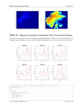
As we can notice in the code, the value of each pixel is converted following the proper equation
in order to get, at the end of the process, the Rainfall Rate R. By summing each sample we must
take in account that each value converted in R is evaluated in mm/h so after the sum and the
linear conversion we need to divide by 60 (minutes in a hour).Here we report the most significant
Cumulative Rain map with standard linear visualization and the equivalent log scale plot that is
more comprehensible (low difference between values of R are badly represented in colour gradient
so we need to compress image’s dynamic with logarithmic scale).
Ferro Demetrio, Minetto Alex Page 22 of 27

25. Radar and Remote Sensing Laboratories
Task 2 - Hourly Cumulative Behaviour from Terrestrial Gauges
Choose the rain gauges from the /gaugedata/raingauges-2012-11-28.txt, extract and plot (in two
different matlab figures) the time series of hourly cumulated rain data (mm) for the overall day.
T = readtable(’raingauges_28-11-2012.txt’,’HeaderLines’,1,’Delimiter’,’t’);
2 G_mat=zeros(7,24);
t=1;
4 for g=1:6
G_Mat(g,:)=T.Var5(t:t+23);
6 subplot(2,3,g)
plot(G_Mat(g,:),’r’)
8 grid on;
Ferro Demetrio, Minetto Alex Page 23 of 27

26. Radar and Remote Sensing Laboratories
title(gauge(g).name,’FontWeight’,’bold’,’FontSize’,11,’FontName’,’Arial’)
10 xlabel(’Hour’,’FontName’,’Arial’)
ylabel(’Rain [mm]’,’FontName’,’Arial’)
12 t=t+24;
end
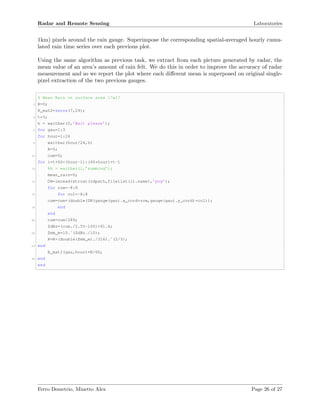
In order to visualize an exhaustive number of realizations of the process, weve reported above the
value collected by six different gauges. We can observe there is some correlation in our graphs,
for sure because the observed area is not so wide to return much uncorrelated profiles of water
precipitation.
Task 3 - Radar Accuracy Analysis
Superimpose in the same plot the hourly cumulated rain observations taken processing radar data
in the pixel where the rain gauge is.
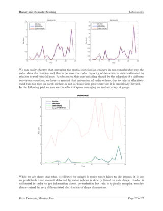
We report below, the map of gauges locations in order to evaluate their position in relation to
meteorological conditions and using the code reported we evaluate the cumulated rain for specific
point of gauges location checking how much precise the radar sensing is.
R=0;
2 R_mat=zeros(7,24);
t=3;
4 h = waitbar(0,’Wait please’);
for gau=1:2
6 for hour=1:24
waitbar(hour/24,h)
8 R=0;
for i=t+60*(hour-1):(60*hour)+t-1
Ferro Demetrio, Minetto Alex Page 24 of 27

27. Radar and Remote Sensing Laboratories
10 %h = waitbar(i,’summing’);
DN=imread(strcat(rdpath,filelist(i).name),’png’);
12 ZdBz=(double(DN(gauge(gau).x_cord,gauge(gau).y_cord))./2.55-100)+91.4;
Zmm_m=10.ˆ(ZdBz./10);
14 R=R+(double(Zmm_m)./316).ˆ(2/3);
end
16 R_mat(gau,hour)=R/60;
end
18
end
20 close(h);
figure(’Name’,’Rain by Gauges’)
22 for i=1:2
24 %subplot(3,3,i)
figure(’Name’,gauge(i).name)
26 plot((R_mat(i,:)),’k’)
hold on;
28 plot(G_Mat(i,:),’r’)
grid on;
30 title(gauge(i).name)
xlabel(’Hour’)
32 ylabel(’Rain [mm]’)
end
As we can see, the result is not very precise. There are several reason for the consistent difference
from radar values and the gauges ones and one of this is proper of precipitation nature. Not all the
water falling at 1 km of altitude falls exactly in the same position it has seen before and above all
most of that water doesn’t fall at all because it can evaporate until to touch the ground.
Task 4 - Spatial Average on Radar Data
Evaluate the effects of spatial-averaging the radar data considering, for each point where each rain
gauge is, the hourly cumulated rain averaged on an area of 9x9 (500m x 500m) and 17x17 (1km x
Ferro Demetrio, Minetto Alex Page 25 of 27

28. Radar and Remote Sensing Laboratories
1km) pixels around the rain gauge. Superimpose the corresponding spatial-averaged hourly cumu-
lated rain time series over each previous plot.
Using the same algorithm as previous task, we extract from each picture generated by radar, the
mean value of an area’s amount of rain felt. We do this in order to improve the accuracy of radar
measurement and so we report the plot where each different mean is superposed on original single-
pixel extraction of the two previous gauges.
% Mean Rain on surface area 17x17
2 R=0;
R_mat2=zeros(7,24);
4 t=3;
h = waitbar(0,’Wait please’);
6 for gau=1:3
for hour=1:24
8 waitbar(hour/24,h)
R=0;
10 cum=0;
for i=t+60*(hour-1):(60*hour)+t-1
12 %h = waitbar(i,’summing’);
mean_rain=0;
14 DN=imread(strcat(rdpath,filelist(i).name),’png’);
for row=-8:8
16 for col=-8:8
cum=cum+(double(DN(gauge(gau).x_cord+row,gauge(gau).y_cord)+col));
18 end
end
20 cum=cum/289;
ZdBz=(cum./2.55-100)+91.4;
22 Zmm_m=10.ˆ(ZdBz./10);
R=R+(double(Zmm_m)./316).ˆ(2/3);
24 end
R_mat2(gau,hour)=R/60;
26 end
end
Ferro Demetrio, Minetto Alex Page 26 of 27

29. Radar and Remote Sensing Laboratories
We can easily observe that averaging the spatial distribution changes in non-considerable way the
radar data distribution and this is because the radar capacity of detection is under-estimated in
relation to real rain-fall rate. A solution on this non-matching should be the adoption of a different
conversion equation; we have to remind that conversion of radar echoes, due to rain in effectively
valid rain fall rate on earth surface, is not a closed form procedure but it is empirically derived.
In the following plot we can see the effect of space averaging on real accuracy of gauge.
While we are shure that what is collected by gauges is really water fallen to the ground, it is not
so predictable that amount detected by radar echoes is strictly linked to rain drops. Radar is
calibrated in order to get information about perturbation but rain is typically complex weather
characterized by very differentiated distribution of drops dimensions.
Ferro Demetrio, Minetto Alex Page 27 of 27