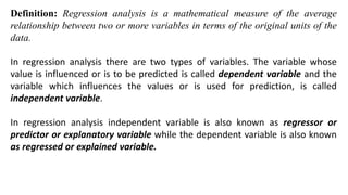
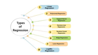
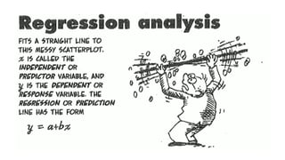
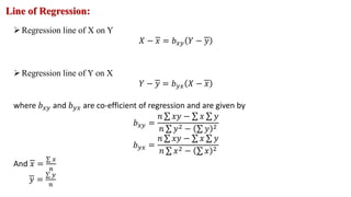
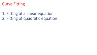
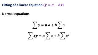
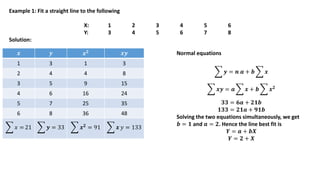
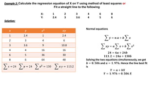
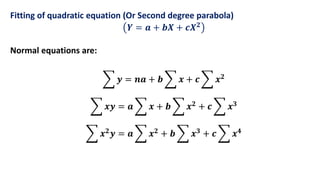
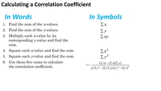
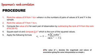
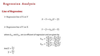
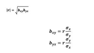
The document provides an overview of regression analysis, detailing its definition, the types of variables involved, and the regression equations used to predict relationships between dependent and independent variables. It includes multiple examples illustrating how to compute regression coefficients, estimate values based on given data, and fit both linear and quadratic equations. Additionally, it discusses correlation coefficients and methods for calculating them, emphasizing the statistical relationship between two variables.

1. Regression Analysis

2. Sir Francis Galton (1822 – 1911)
Sir Francis Galton was an English Victoria
era statistician, polymath, sociologist, psychologist, anthropologist,
eugenicist, tropical explorer, geographer, inventor, meteorologist,
proto-geneticist, and psychometrician. He was knighted in 1909

3. Definition: Regression analysis is a mathematical measure of the average
relationship between two or more variables in terms of the original units of the
data.
In regression analysis there are two types of variables. The variable whose
value is influenced or is to be predicted is called dependent variable and the
variable which influences the values or is used for prediction, is called
independent variable.
In regression analysis independent variable is also known as regressor or
predictor or explanatory variable while the dependent variable is also known
as regressed or explained variable.

7. Line of Regression:
Regression line of X on Y
𝑋 − 𝑥 = 𝑏𝑥𝑦 𝑌 − 𝑦
Regression line of Y on X
𝑌 − 𝑦 = 𝑏𝑦𝑥 𝑋 − 𝑥
where 𝑏𝑥𝑦 and 𝑏𝑦𝑥 are co-efficient of regression and are given by
𝑏𝑥𝑦 =
𝑛 𝑥𝑦 − 𝑥 𝑦
𝑛 𝑦2 − 𝑦 2
𝑏𝑦𝑥 =
𝑛 𝑥𝑦 − 𝑥 𝑦
𝑛 𝑥2 − 𝑥 2
And 𝑥 =
𝑥
𝑛
𝑦 =
𝑦
𝑛

8. Note: The geometric mean of the two regression co-
efficients is numerically equal to correlation co-efficient
I.e., 𝒃𝒙𝒚𝒃𝒚𝒙 = 𝒓

9. Problems on
Regression Analysis

10. Example 1: The following table gives the age of cars of a certain make and annual maintenance costs
(i) Obtain the two regression equation
(ii) What would be the cost maintenance given that the car is 5 years old
Age of cars (in years): 2 4 6 8
Maintenance cost (in hundreds of Rs.): 10 20 25 30
Solution:
Let X: age of cars in years and, Y: maintenance cost
𝒙 𝒚 𝒙𝟐 𝒚𝟐 𝒙𝒚
2 10 4 100 20
4 20 16 400 80
6 25 36 625 150
8 30 64 900 240
𝒙 = 𝟐𝟎 𝒚 = 𝟖𝟓 𝒙𝟐 = 𝟏𝟐𝟎 𝒚𝟐 = 𝟐𝟎𝟐𝟓 𝒙𝒚 = 𝟒𝟗𝟎

11. (i) 𝒙 =
𝒙
𝒏
=
20
4
= 5 years
𝒚 =
𝒚
𝒏
=
85
4
= 21.25 (hundred Rs.)
co-efficient of regression,
𝒃𝒙𝒚 =
𝒏 𝒙𝒚 − 𝒙 𝒚
𝒏 𝒚𝟐 − 𝒚 𝟐
4 490 − 20 85
4 2025 − 85 2 = 0.297
𝒃𝒚𝒙 =
𝒏 𝒙𝒚− 𝒙 𝒚
𝒏 𝒙𝟐− 𝒙 𝟐
=
4 490 − 20 85
4 120 − 20 2 = 3.25
 Regression line of X on Y
𝑿 − 𝒙 = 𝒃𝒙𝒚 𝒀 − 𝒚
𝑋 − 5 = 0.297 + 𝑌 − 21.25
𝑋 = 0.297 𝑌 − 1.31
 Regression line of Y on X
𝒀 − 𝒚 = 𝒃𝒚𝒙 𝑿 − 𝒙
𝑌 − 21.25 = 3.25 𝑋 − 5
𝑌 = 3.25 𝑋 + 5
(ii) To calculate the cost of maintenance when the age of case is 5 years (i.e., given X=5, Y= ? ). We use the
Regression line of Y on X
𝒀 = 𝟑. 𝟐𝟓 𝑿 + 𝟓 = 3.25 5 + 5 = 21.25 (𝑖𝑛 ℎ𝑢𝑛𝑑𝑟𝑒𝑑 𝑅𝑠. )

12. Example 1: Find the lines of regression using the following. Hence estimate the value of Y when X=30 and X when Y=16
x: 21 23 24 28 29 31 34
y: 11 12 14 15 17 18 19
Solution:
Let X: age of cars in years and, Y: maintenance cost
𝒙 𝒚 𝒙𝟐 𝒚𝟐 𝒙𝒚
21 11
23 12
24 14
28 15
29 17
31 18
34 19
𝒙 = 𝒚 = 𝒙𝟐 = 𝒚𝟐 = 𝒙𝒚 =

13. 𝒙 =
𝒙
𝒏
=
𝒚 =
𝒚
𝒏
=
co-efficient of regression,
𝒃𝒙𝒚 =
𝒏 𝒙𝒚 − 𝒙 𝒚
𝒏 𝒚𝟐 − 𝒚 𝟐
𝒃𝒚𝒙 =
𝒏 𝒙𝒚− 𝒙 𝒚
𝒏 𝒙𝟐− 𝒙 𝟐
 Regression line of X on Y
𝑿 − 𝒙 = 𝒃𝒙𝒚 𝒀 − 𝒚
 Regression line of Y on X
𝒀 − 𝒚 = 𝒃𝒚𝒙 𝑿 − 𝒙
To estimate the value of Y when X=30, we use the regression of Y on X
𝒀 =
To estimate the value of X when Y=16, we use the regression of X on Y
𝑿 =

14. Example 3:
In a bivariate data, the regression co-efficients are -
0.333 and -0.75. Find the co-efficient of correlation
𝒓 = 𝒃𝒙𝒚𝒃𝒚𝒙 = −𝟎. 𝟑𝟑𝟑 −𝟎. 𝟕𝟓 = 𝟎. 𝟓
Since the regression co-efficients are negative, the
correlation co-efficient also has to be negative.
Hence 𝑟 = −.05

15. Example 4: In a bivariate data, 𝑥 = 20, 𝑦 = 15, 𝜎𝑥 = 4, 𝜎𝑦 = 3
and 𝑟 = 0.7. Obtain the two regression lines and estimate 𝑌
when 𝑋 = 24
Solution: The regression co-efficients
𝒃𝒙𝒚 = 𝒓
𝝈𝒙
𝝈𝒚
=
𝟎. 𝟕(𝟒)
𝟑
= 𝟎. 𝟗𝟑𝟑
𝒃𝒚𝒙 = 𝒓
𝝈𝒚
𝝈𝒙
=
𝟎. 𝟕(𝟑)
𝟒
= 𝟎. 𝟓𝟐𝟓

16.  Regression line of X on Y
𝑿 − 𝒙 = 𝒃𝒙𝒚 𝒀 − 𝒚
𝑿 − 𝟐𝟎 = 𝟎. 𝟗𝟑𝟑 𝒀 − 𝟏𝟓
𝑿 = 𝟎. 𝟗𝟑𝟑 𝒀 + 𝟔. 𝟎𝟎𝟓
 Regression line of Y on X
𝒀 − 𝒚 = 𝒃𝒚𝒙 𝑿 − 𝒙
𝒀 − 𝟏𝟓 = 𝟎. 𝟓𝟐𝟓 𝑿 − 𝟐𝟎
𝒀 = 𝟎. 𝟓𝟐𝟓 𝑿 + 𝟒. 𝟓
To estimate the value of Y when X=24, we use the regression of Y on X
𝒀 = 𝟎. 𝟓𝟐𝟓 𝑿 + 𝟒. 𝟓
= 0.525 24 + 4.5 = 17.1

17. Curve Fitting
1. Fitting of a linear equation
2. Fitting of quadratic equation

18. Fitting of a linear equation (𝒚 = 𝒂 + 𝒃𝒙)
Normal equations
𝒚 = 𝒏 𝒂 + 𝒃 𝒙
𝒙𝒚 = 𝒂 𝒙 + 𝒃 𝒙𝟐

19. Example 1: Fit a straight line to the following
X: 1 2 3 4 5 6
Y: 3 4 5 6 7 8
Solution:
𝒙 𝒚 𝒙𝟐 𝒙𝒚
1 3 1 3
2 4 4 8
3 5 9 15
4 6 16 24
5 7 25 35
6 8 36 48
𝑥 = 21 𝒚 = 33 𝒙𝟐
= 91 𝒙 𝑦 = 133
Normal equations
𝒚 = 𝒏 𝒂 + 𝒃 𝒙
𝒙𝒚 = 𝒂 𝒙 + 𝒃 𝒙𝟐
𝟑𝟑 = 𝟔𝒂 + 𝟐𝟏𝒃
𝟏𝟑𝟑 = 𝟐𝟏𝒂 + 𝟗𝟏𝒃
Solving the two equations simultaneously, we get
𝒃 = 𝟏 and 𝒂 = 𝟐. Hence the line best fit is
𝒀 = 𝒂 + 𝒃𝑿
𝒀 = 𝟐 + 𝑿

20. Example 2: Calculate the regression equation of X on Y using method of least squares or
Fit a straight line to the following
X: 1 2 3 4 6 8
Y: 2.4 3 3.6 4 5 6
Solution:
𝒙 𝒚 𝒙𝟐 𝒙𝒚
1 2.4 1 2.4
2 3 4 6
3 3.6 9 10.8
4 4 16 16
6 5 36 30
8 6 64 48
𝑥 = 24 𝒚 = 24 𝒙𝟐
= 130 𝒙 𝑦 = 113.2
Normal equations
𝒚 = 𝒏 𝒂 + 𝒃 𝒙
𝒙𝒚 = 𝒂 𝒙 + 𝒃 𝒙𝟐
𝟐𝟒 = 𝟔𝒂 + 𝟐𝟒𝒃
𝟏𝟏𝟑. 𝟐 = 𝟐𝟒𝒂 + 𝟏𝟑𝟎𝒃
Solving the two equations simultaneously, we get
𝒃 = 𝟎. 𝟓𝟎𝟔 and 𝒂 = 𝟏. 𝟗𝟕𝟔. Hence the line best fit
is
𝒀 = 𝒂 + 𝒃𝑿
𝒀 = 𝟏. 𝟗𝟕𝟔 + 𝟎. 𝟓𝟎𝟔 𝑿

22. Fitting of quadratic equation

23. Fitting of quadratic equation (Or Second degree parabola)
𝒀 = 𝒂 + 𝒃𝑿 + 𝒄𝑿𝟐
Normal equations are:
𝒚 = 𝒏𝒂 + 𝒃 𝒙 + 𝒄 𝒙𝟐
𝒙𝒚 = 𝒂 𝒙 + 𝒃 𝒙𝟐 + 𝒄 𝒙𝟑
𝒙𝟐
𝒚 = 𝒂 𝒙𝟐
+ 𝒃 𝒙𝟑
+ 𝒄 𝒙𝟒

24. Example 3: Fit a second degree parabola to the following data:
X: 1 2 3 4 5 6 7 8 9
Y: 2 6 7 8 10 11 11 10 9
Solution:
Let the parabola of best fit be 𝒀 = 𝒂 + 𝒃𝑿 + 𝒄𝑿𝟐.
Let 𝑼 = 𝑿 − 𝟓 and 𝑽 = 𝒀 − 𝟖
Now the parabola of best fit is 𝑽 = 𝒂 + 𝒃𝑼 + 𝒄𝑼𝟐
𝐱 𝐲 𝐮 𝐯 𝒖𝒗 𝒖𝟐
𝒖𝟐
𝒗 𝒖𝟑 𝒖𝟒

25. 𝒙 𝒚 𝒖 𝒗 𝒖𝒗 𝒖𝟐
𝒖𝟐
𝒗 𝒖𝟑 𝒖𝟒
1 2 -4 -6 21 16 -96 -64 256
2 6 -3 -2 6 9 -18 -27 81
3 7 -2 -1 2 4 -4 -8 16
4 8 -1 0 0 1 0 -1 1
5 10 0 2 0 0 0 0 0
6 11 1 3 3 1 3 1 1
7 11 2 3 6 4 12 8 16
8 10 3 2 6 9 18 27 81
9 9 4 1 4 16 16 64 256
0 2 51 60 -69 0 708
Normal equations are:
𝒗 = 𝒏𝒂 + 𝒃 𝒖 + 𝒄 𝒖𝟐
𝒖𝒗 = 𝒂 𝒖 + 𝒃 𝒖𝟐
+ 𝒄 𝒖𝟑
𝒖𝟐
𝒗 = 𝒂 𝒖𝟐
+ 𝒃 𝒖𝟑
+ 𝒄 𝒖𝟒
𝟐 = 𝟗𝒂 + 𝟎 + 𝟔𝟎𝒄
𝟓𝟏 = 𝟎 + 𝟔𝟎𝒃 + 𝟎
−𝟔𝟗 = 𝟔𝟎𝒂 + 𝟎 + 𝟕𝟎𝟖𝒄
Solving the equations simultaneously, we get 𝒂 =
− 𝟏. 𝟓𝟓, 𝒃 = 𝟎. 𝟖𝟓 and 𝒄 = −𝟎. 𝟏𝟒
𝑽 = −𝟏. 𝟓𝟓 + 𝟎. 𝟖𝟓𝑼 − 𝟎. 𝟐𝟔𝟓𝑼𝟐
𝒀 − 𝟖 = −𝟏. 𝟓𝟓 + 𝟎. 𝟖𝟓 𝒙 − 𝟓 − 𝟎. 𝟏𝟒 𝑿 − 𝟓 𝟐

27. CORRELATION
Correlation coefficient: statistical index of the degree to which two variables are associated, or related

28. Karl Pearson’s Coefficient Correlation
The formula for computing Pearson Coefficient Correlation (r) is:
  
   
2 2
2 2
.
n xy x y
r
n x x n y y
   

     
Calculating a Correlation Coefficient
In Words In Symbols
x

y

xy

2
x

2
y

  
   
2 2
2 2
.
n xy x y
r
n x x n y y
   

     
1. Find the sum of the x-values.
2. Find the sum of the y-values.
3. Multiply each x-value by its
corresponding y-value and find the
sum.
4. Square each x-value and find the sum.
5. Square each y-value and find the sum.
6. Use these five sums to calculate
the correlation coefficient.

29. Calculating a Correlation Coefficient
In Words In Symbols
x

y

xy

2
x

2
y

  
   
2 2
2 2
.
n xy x y
r
n x x n y y
   

     
1. Find the sum of the x-values.
2. Find the sum of the y-values.
3. Multiply each x-value by its
corresponding y-value and find the
sum.
4. Square each x-value and find the sum.
5. Square each y-value and find the sum.
6. Use these five sums to calculate
the correlation coefficient.

30. Spearman’s rank correlation
PROCEDURE
1. Rank the values of X from 1 to n where n is the numbers of pairs of values of X and Y in the
sample.
2. Rank the values of Y from 1 to n.
3. Compute the value of di for each pair of observation by subtracting the rank of Yi from the rank
of Xi (Xi-Yi)
4. Square each di and compute 𝑑𝑖2 which is the sum of the squared values.
5. Apply the following formula
1)
n(n
(di)
6
1
r 2
2
s




The value of rs denotes the magnitude and nature of
association giving the same interpretation as simple r.

31. Line of Regression:
 Regression line of X on Y
𝑋 − 𝑥 = 𝑏𝑥𝑦 𝑌 − 𝑦
 Regression line of Y on X
𝑌 − 𝑦 = 𝑏𝑦𝑥 𝑋 − 𝑥
where 𝑏𝑥𝑦 and 𝑏𝑦𝑥 are co-efficient of regression and are given by
𝑏𝑥𝑦 =
𝑛 𝑥𝑦 − 𝑥 𝑦
𝑛 𝑦2 − 𝑦 2
𝑏𝑦𝑥 =
𝑛 𝑥𝑦 − 𝑥 𝑦
𝑛 𝑥2 − 𝑥 2
And 𝑥 =
𝑥
𝑛
𝑦 =
𝑦
𝑛
R e g r e s s i o n A n a l y s i s

32. 𝒓 = 𝒃𝒙𝒚𝒃𝒚𝒙
𝒃𝒙𝒚 = 𝒓
𝝈𝒙
𝝈𝒚
𝒃𝒚𝒙 = 𝒓
𝝈𝒚
𝝈𝒙

33. Fitting of a linear equation (𝒚 = 𝒂 + 𝒃𝒙)
Normal equations
𝒚 = 𝒏 𝒂 + 𝒃 𝒙
𝒙𝒚 = 𝒂 𝒙 + 𝒃 𝒙𝟐

34. Fitting of quadratic equation (Or Second degree parabola)
𝒀 = 𝒂 + 𝒃𝑿 + 𝒄𝑿𝟐
Normal equations are:
𝒚 = 𝒏𝒂 + 𝒃 𝒙 + 𝒄 𝒙𝟐
𝒙𝒚 = 𝒂 𝒙 + 𝒃 𝒙𝟐 + 𝒄 𝒙𝟑
𝒙𝟐
𝒚 = 𝒂 𝒙𝟐
+ 𝒃 𝒙𝟑
+ 𝒄 𝒙𝟒