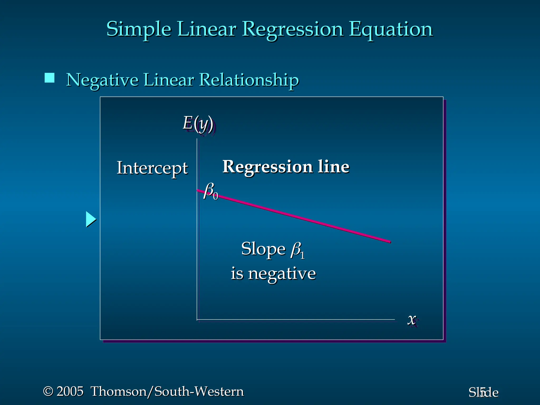
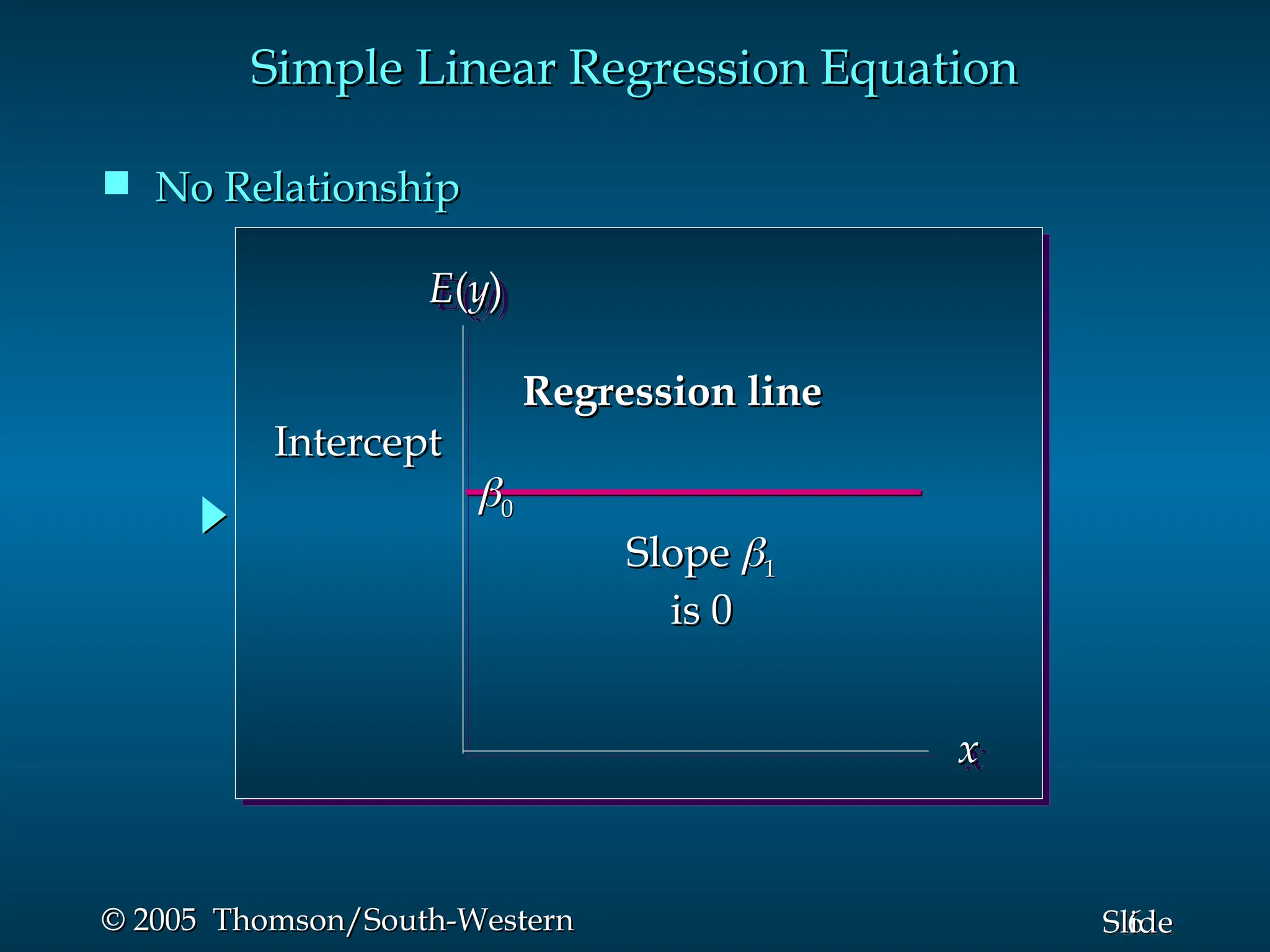
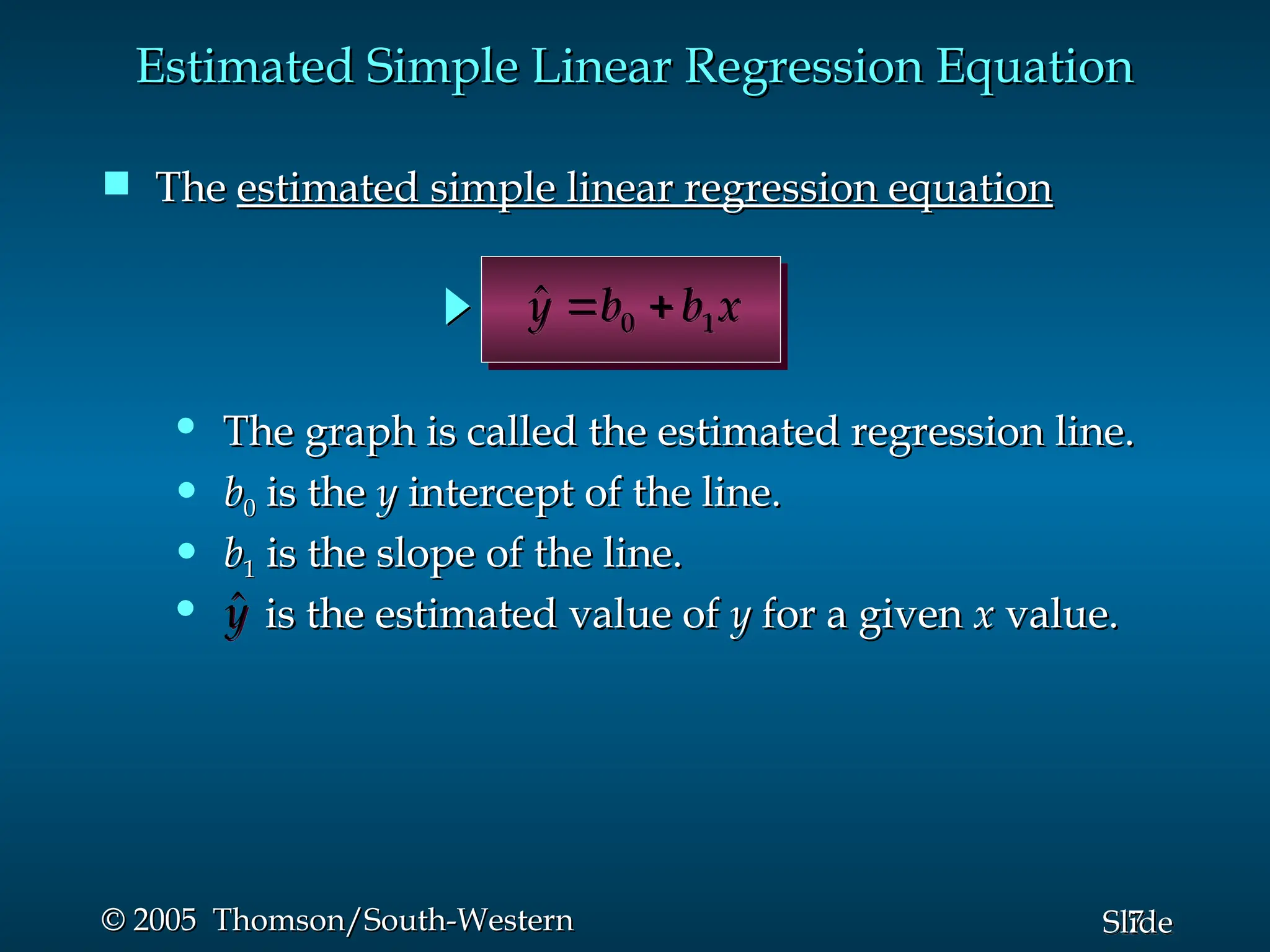
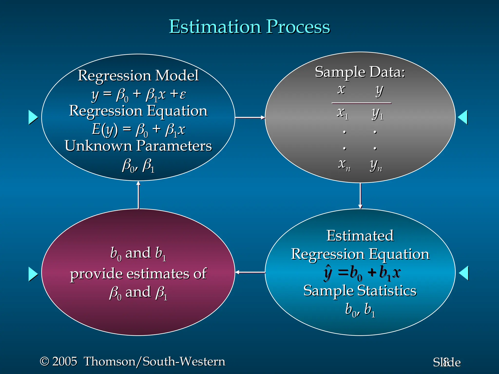
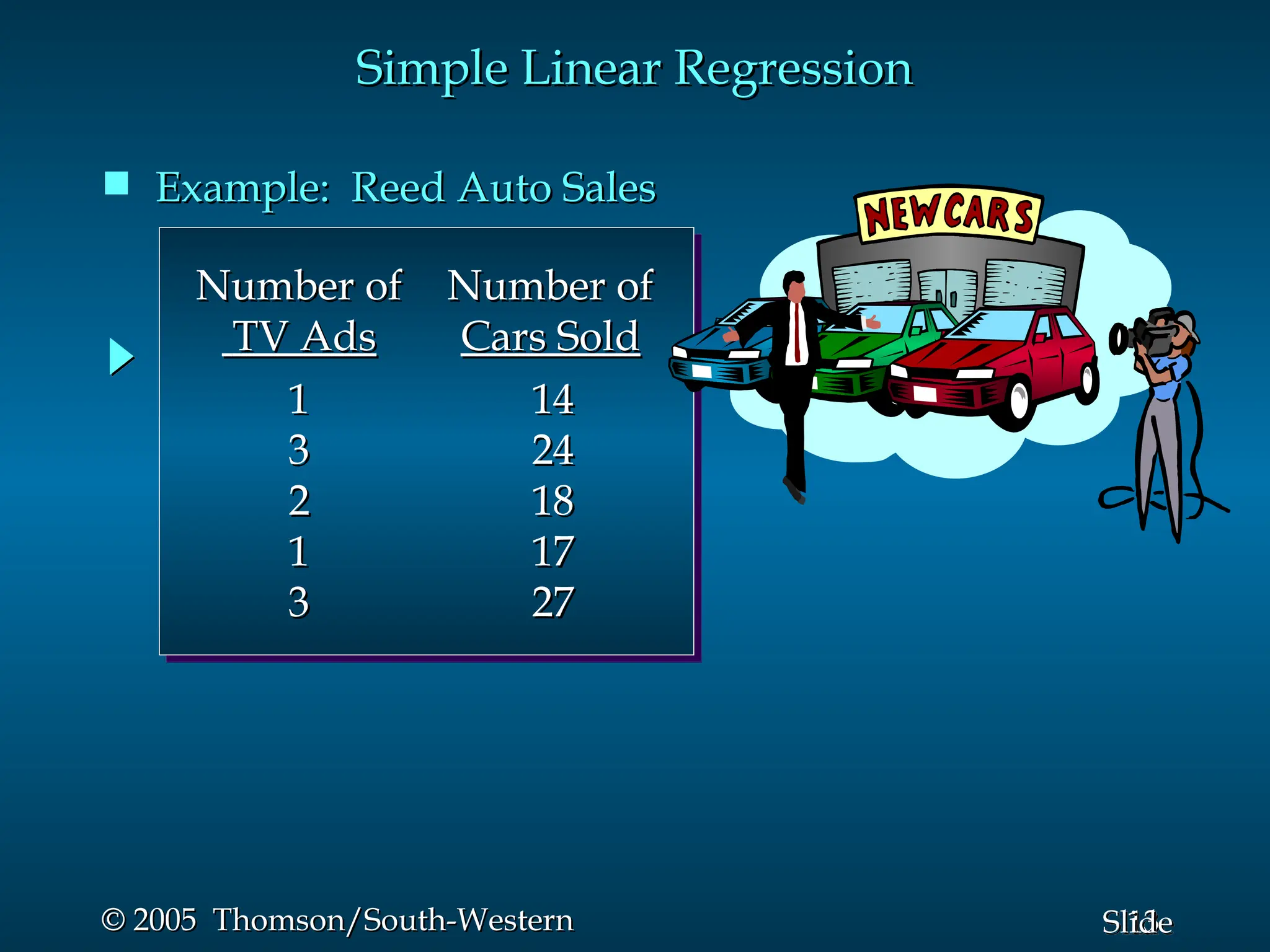
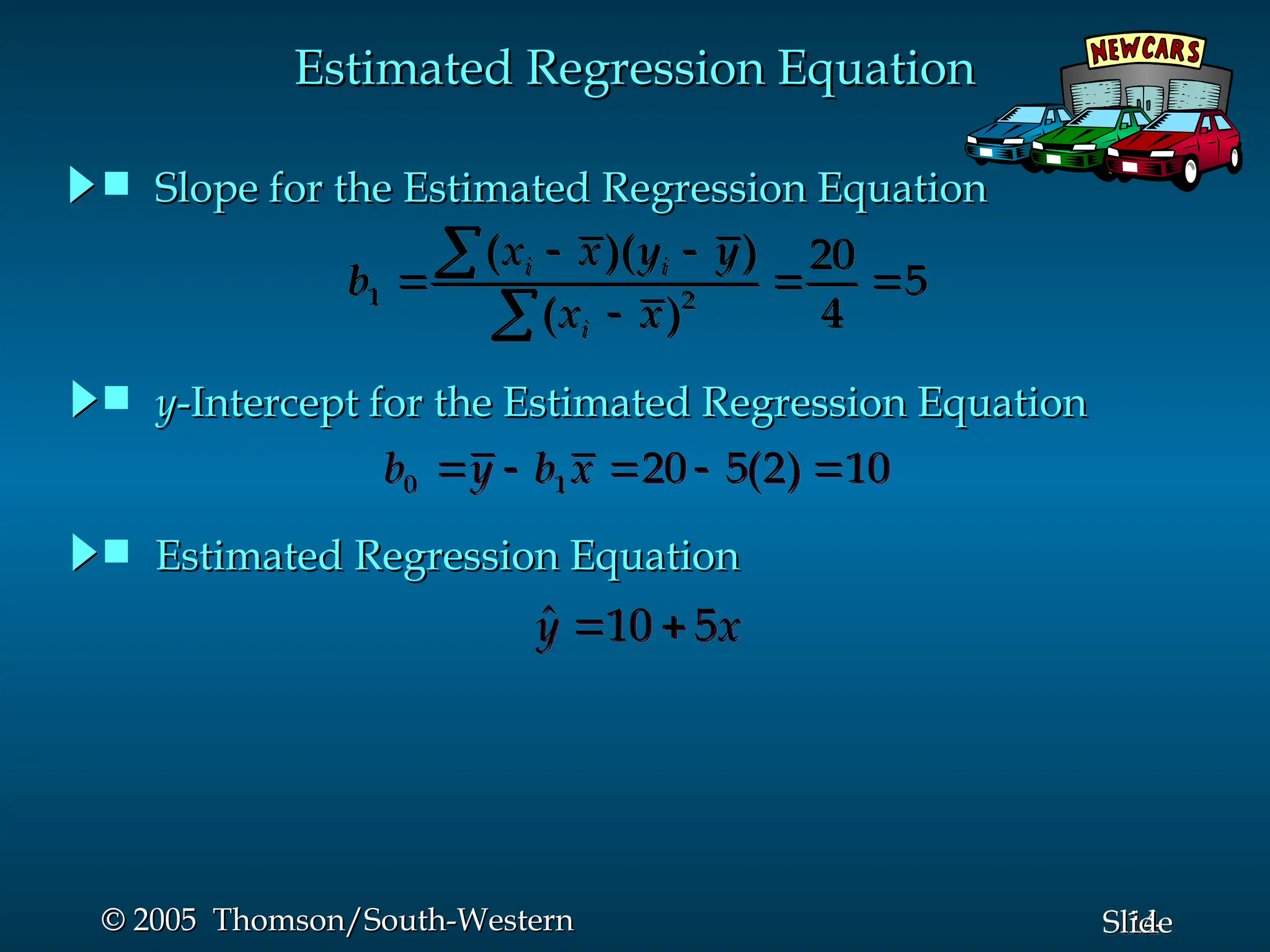
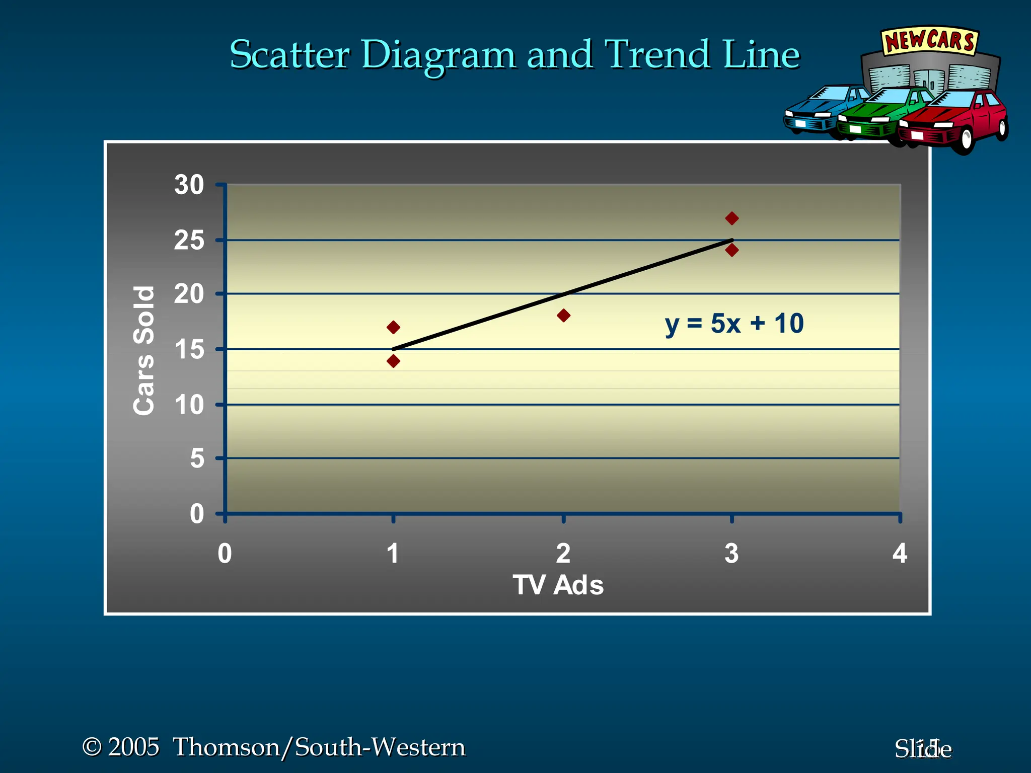
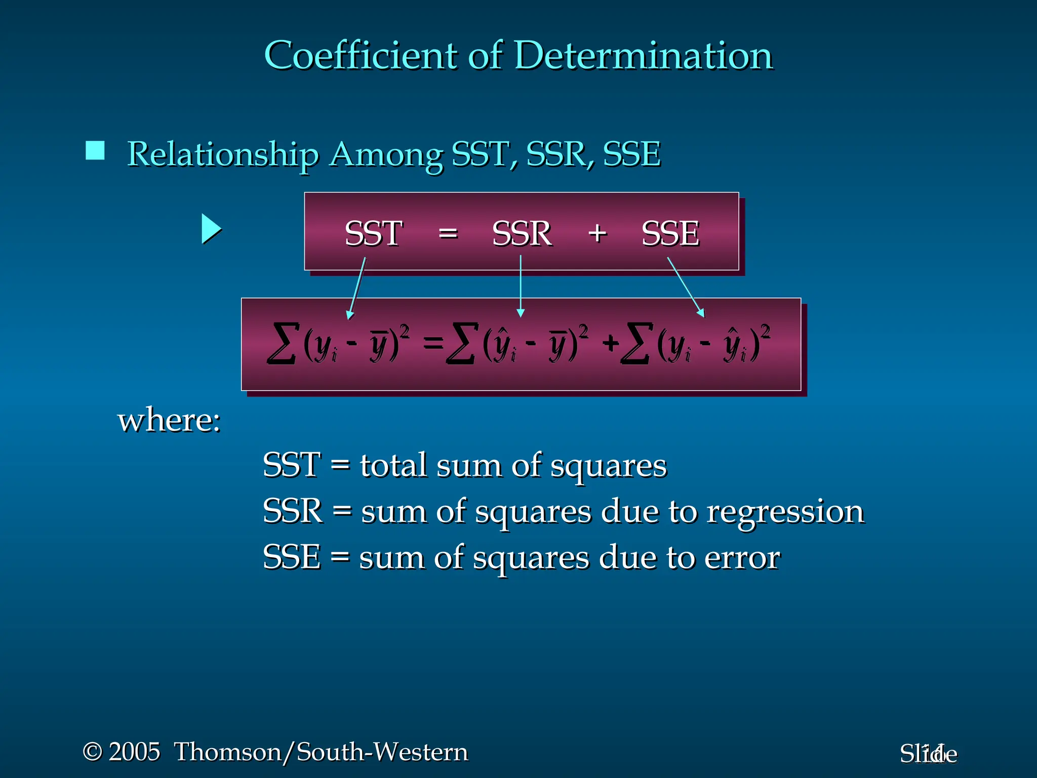
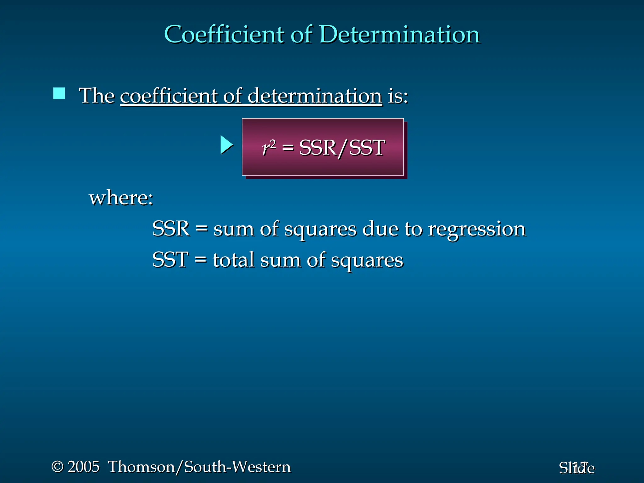
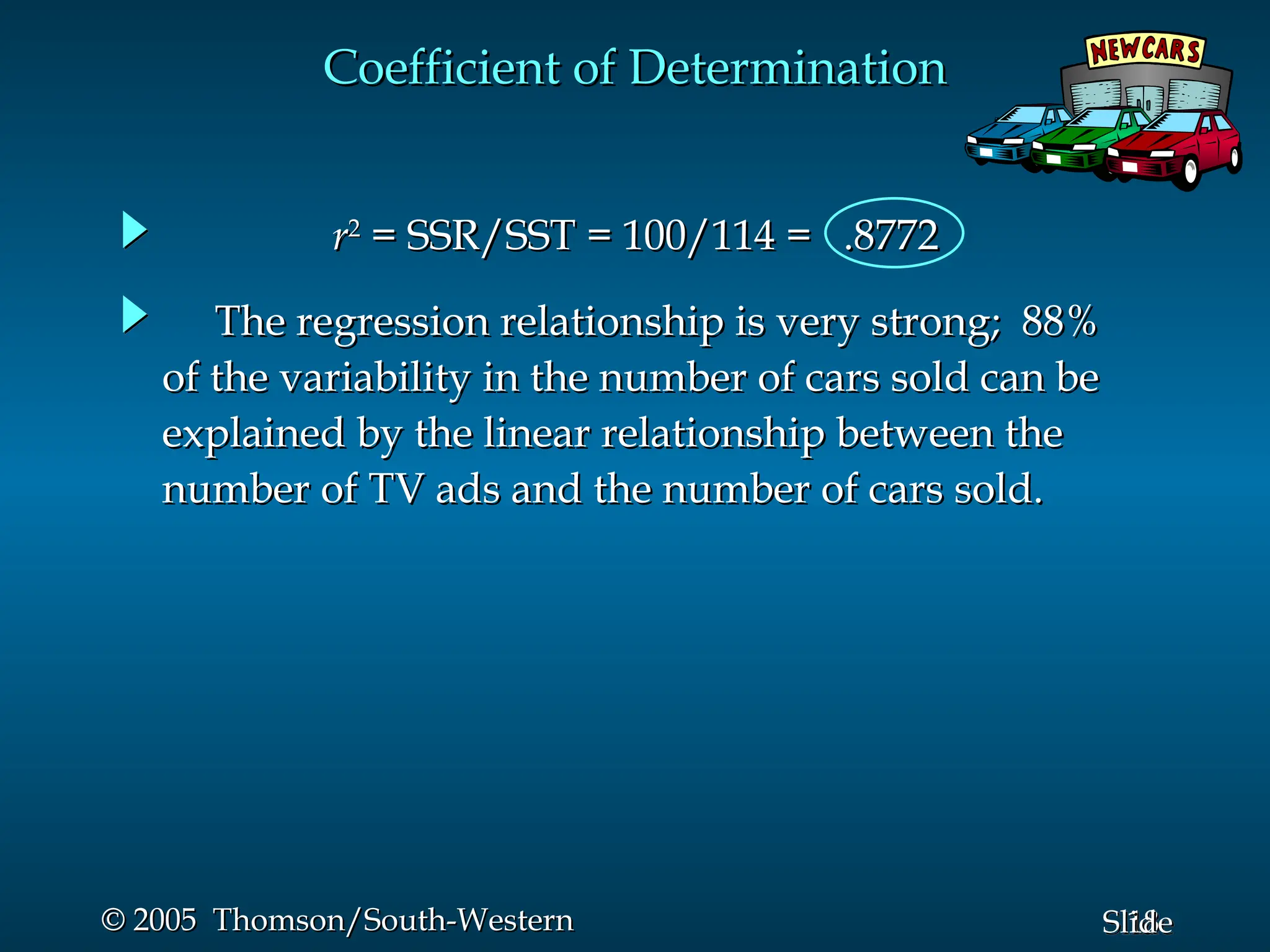
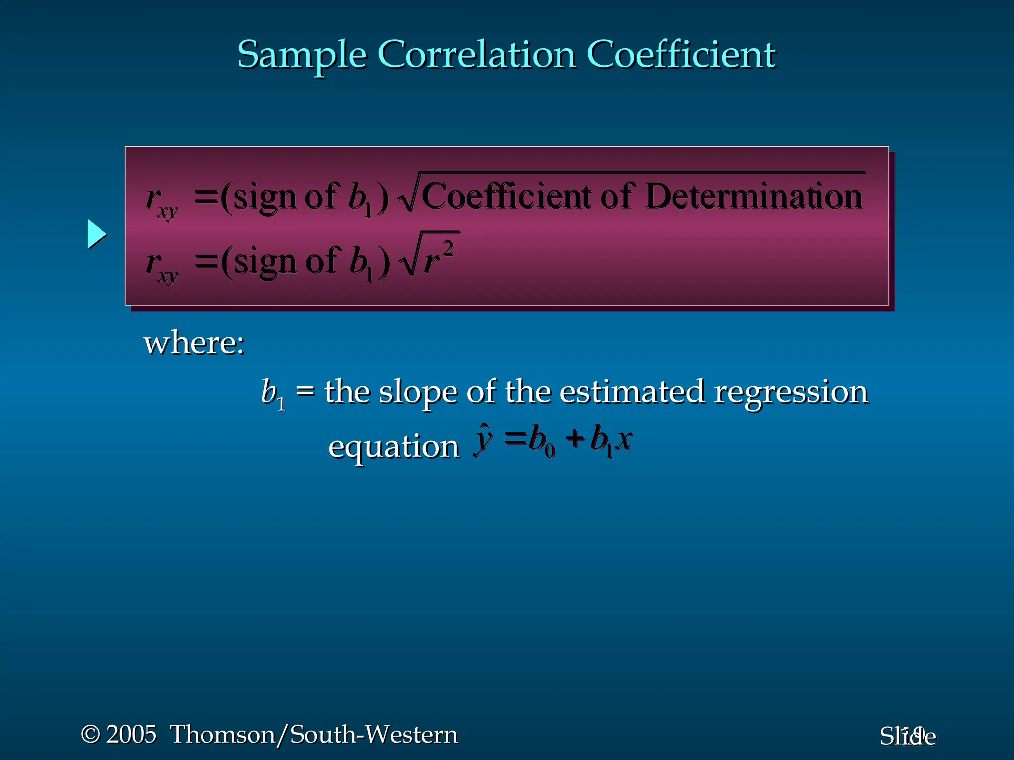
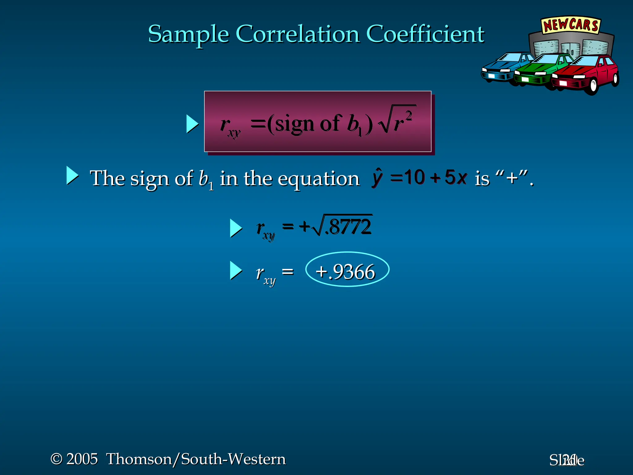
wwwwwwwwwwwwwwwwwwwwW7_Simple_linear_regression_PPT.ppt

1
Slide
© 2005 Thomson/South-Western
Chapter 14
Chapter 14
Simple Linear Regression
 Simple Linear Regression Model
Simple Linear Regression Model
 Least Squares Method
Least Squares Method
 Coefficient of Determination
Coefficient of Determination
 Model Assumptions
Model Assumptions
 Testing for Significance
Testing for Significance
 Using the Estimated Regression Equation
Using the Estimated Regression Equation
for Estimation and Prediction
for Estimation and Prediction
 Computer Solution
Computer Solution
 Residual Analysis: Validating Model Assumptions
Residual Analysis: Validating Model Assumptions

2
Slide
y
y =
= 
0
0 +
+ 
1
1x
x +
+

where:
where:

0
0 and
and 
1
1 are called
are called parameters of the model
parameters of the model,
,

 is a random variable called the
is a random variable called the error term
error term.
.
 The
The simple linear regression model
simple linear regression model is:
is:
 The equation that describes how
The equation that describes how y
y is related to
is related to x
x and
and
an error term is called the
an error term is called the regression model
regression model.
.

3
Slide
Simple Linear Regression Equation
 The
The simple linear regression equation
simple linear regression equation is:
is:
• E
E(
(y
y) is the expected value of
) is the expected value of y
y for a given
for a given x
x value.
value.
• 
1
1 is the slope of the regression line.
is the slope of the regression line.
• 
0
0 is the
is the y
y intercept of the regression line.
intercept of the regression line.
• Graph of the regression equation is a straight line.
Graph of the regression equation is a straight line.
E
E(
(y
y) =
) = 
0
0 +
+ 
1
1x
x

4
Slide
 Positive Linear Relationship
Positive Linear Relationship
E
E(
(y
y)
)
x
x
Slope
Slope 
1
1
is positive
is positive
Regression line
Regression line
Intercept
Intercept

0
0

5
Slide
 Negative Linear Relationship
Negative Linear Relationship
E
E(
(y
y)
)
x
x
Slope
Slope 
1
1
is negative
is negative
Regression line
Regression line
Intercept
Intercept

0
0

6
Slide
 No Relationship
No Relationship
E
E(
(y
y)
)
x
x
Slope
Slope 
1
1
is 0
is 0
Regression line
Regression line
Intercept
Intercept

0
0

7
Slide
Estimated Simple Linear Regression Equation
Estimated Simple Linear Regression Equation
 The
The estimated simple linear regression equation
estimated simple linear regression equation
0 1
ŷ b b x
 
• is the estimated value of
is the estimated value of y
y for a given
for a given x
x value.
value.
ŷ
• b
b1
1 is the slope of the line.
is the slope of the line.
• b
b0
0 is the
is the y
y intercept of the line.
intercept of the line.
• The graph is called the estimated regression line.
The graph is called the estimated regression line.

8
Slide
Estimation Process
Estimation Process
Regression Model
Regression Model
y
y =
= 
0
0 +
+ 
1
1x
x +
+

Regression Equation
Regression Equation
E
E(
(y
y) =
) = 
0
0 +
+ 
1
1x
x
Unknown Parameters
Unknown Parameters

0
0,
, 
1
1
Sample Data:
Sample Data:
x y
x y
x
x1
1 y
y1
1
. .
. .
. .
. .
x
xn
n y
yn
n
b
b0
0 and
and b
b1
1
provide estimates of
provide estimates of

0
0 and
and 
1
1
Estimated
Estimated
Regression Equation
Regression Equation
Sample Statistics
Sample Statistics
b
b0
0,
, b
b1
1
0 1
ŷ b b x
 

9
Slide
 Least Squares Criterion
Least Squares Criterion
min (y y
i i

  )2
where:
where:
y
yi
i =
= observed
observed value of the dependent variable
value of the dependent variable
for the
for the i
ith observation
th observation
^
^
y
yi
i =
= estimated
estimated value of the dependent variable
value of the dependent variable
for the
for the i
ith observation
th observation

10
Slide
 Slope for the Estimated Regression Equation
Slope for the Estimated Regression Equation
1 2
( )( )
( )
i i
i
x x y y
b
x x
 





11
Slide
 y
y-Intercept for the Estimated Regression Equation
-Intercept for the Estimated Regression Equation
0 1
b y b x
 
where:
where:
x
xi
i = value of independent variable for
= value of independent variable for i
ith
th
observation
observation
n
n = total number of observations
= total number of observations
_
_
y
y = mean value for dependent variable
= mean value for dependent variable
_
_
x
x = mean value for independent variable
= mean value for independent variable
y
yi
i = value of dependent variable for
= value of dependent variable for i
ith
th
observation
observation

12
Slide
Reed Auto periodically has
Reed Auto periodically has
a special week-long sale.
a special week-long sale.
As part of the advertising
As part of the advertising
campaign Reed runs one or
campaign Reed runs one or
more television commercials
more television commercials
during the weekend preceding the sale. Data from a
during the weekend preceding the sale. Data from a
sample of 5 previous sales are shown on the next slide.
sample of 5 previous sales are shown on the next slide.
 Example: Reed Auto Sales
Example: Reed Auto Sales

13
Slide
 Example: Reed Auto Sales
Example: Reed Auto Sales
Number of
Number of
TV Ads
TV Ads
Number of
Number of
Cars Sold
Cars Sold
1
1
3
3
2
2
1
1
3
3
14
14
24
24
18
18
17
17
27
27

14
Slide
Estimated Regression Equation
ˆ 10 5
y x
 
1 2
( )( ) 20
5
( ) 4
i i
i
x x y y
b
x x
 
  



0 1 20 5(2) 10
b y b x
    
 Slope for the Estimated Regression Equation
Slope for the Estimated Regression Equation
 y
y-Intercept for the Estimated Regression Equation
-Intercept for the Estimated Regression Equation
 Estimated Regression Equation

15
Slide
Scatter Diagram and Trend Line
Scatter Diagram and Trend Line
y = 5x + 10
0
5
10
15
20
25
30
0 1 2 3 4
TV Ads
Cars
Sold

16
Slide
 Relationship Among SST, SSR, SSE
Relationship Among SST, SSR, SSE
where:
where:
SST = total sum of squares
SSR = sum of squares due to regression
SSE = sum of squares due to error
SSE = sum of squares due to error
SST = SSR + SSE
SST = SSR + SSE
2
( )
i
y y

 2
ˆ
( )
i
y y
 
 2
ˆ
( )
i i
y y
 


17
Slide
 The
The coefficient of determination
coefficient of determination is:
is:
where:
where:
r
r2
2
= SSR/SST
= SSR/SST

18
Slide
r
r2
2
= SSR/SST = 100/114 = .8772
= SSR/SST = 100/114 = .8772
The regression relationship is very strong; 88%
The regression relationship is very strong; 88%
of the variability in the number of cars sold can be
of the variability in the number of cars sold can be
explained by the linear relationship between the
explained by the linear relationship between the
number of TV ads and the number of cars sold.
number of TV ads and the number of cars sold.

19
Slide
Sample Correlation Coefficient
2
1)
of
(sign r
b
rxy 
ion
Determinat
of
t
Coefficien
)
of
(sign 1
b
rxy 
where:
where:
b
b1
1 = the slope of the estimated regression
= the slope of the estimated regression
equation
equation x
b
b
y 1
0
ˆ 


20
Slide
2
1)
of
(sign r
b
rxy 
The sign of
The sign of b
b1
1 in the equation
in the equation is “+”.
is “+”.
ˆ 10 5
y x
 
= + .8772
xy
r
r
rxy
xy = +.9366
= +.9366

21
Slide
Assumptions About the Error Term
Assumptions About the Error Term 

1. The error
1. The error 
 is a random variable with mean of zero.
is a random variable with mean of zero.
2. The variance of
2. The variance of 
 , denoted by
, denoted by 
2
2
, is the same for
, is the same for
all values of the independent variable.
all values of the independent variable.
3. The values of
3. The values of 
 are independent.
are independent.
4. The error
4. The error 
 is a normally distributed random
is a normally distributed random
variable.
variable.

22
Slide
To test for a significant regression relationship, we
To test for a significant regression relationship, we
must conduct a hypothesis test to determine whether
must conduct a hypothesis test to determine whether
the value of
the value of 
1
1 is zero.
is zero.
Two tests are commonly used:
Two tests are commonly used:
t
t Test
Test and
and F
F Test
Test
Both the
Both the t
t test and
test and F
F test require an estimate of
test require an estimate of 

2
2
,
,
the variance of
the variance of 

 in the regression model.
in the regression model.

23
Slide
 An Estimate of
An Estimate of 


 



 2
1
0
2
)
(
)
ˆ
(
SSE i
i
i
i x
b
b
y
y
y
where:
where:
s
s2
2
= MSE = SSE/(
= MSE = SSE/(n
n 
 2)
2)
The mean square error (MSE) provides the estimate
The mean square error (MSE) provides the estimate
of
of 
 2
2
, and the notation
, and the notation s
s2
2
is also used.
is also used.

24
Slide
 An Estimate of
An Estimate of 

2
SSE
MSE



n
s
• To estimate
To estimate 
 we take the square root of
we take the square root of 
2
2
.
.
• The resulting
The resulting s
s is called the
is called the standard error of
standard error of
the estimate
the estimate.
.

25
Slide
 Hypotheses
Hypotheses
 Test Statistic
Test Statistic
Testing for Significance:
Testing for Significance: t
t Test
Test
0 1
: 0
H  
1
: 0
a
H  
1
1
b
b
t
s


26
Slide
 Rejection Rule
Rejection Rule
t Test
Test
where:
where:
t
t

 is based on a
is based on a t
t distribution
distribution
with
with n
n - 2 degrees of freedom
- 2 degrees of freedom
Reject
Reject H
H0
0 if
if p
p-value
-value <
< 

or
or t
t <
< -
-t
t

or
or t
t >
> t
t



27
Slide
1. Determine the hypotheses.
2. Specify the level of significance.
3. Select the test statistic.

 = .05
= .05
4. State the rejection rule.
4. State the rejection rule. Reject
Reject H
H0
0 if
if p
p-value
-value <
< .05
.05
or |
or |t|
t| > 3.182 (with
> 3.182 (with
3 degrees of freedom)
3 degrees of freedom)
t Test
Test
0 1
: 0
H  
1
: 0
a
H  
1
1
b
b
t
s


28
Slide
t Test
Test
5. Compute the value of the test statistic.
6. Determine whether to reject
6. Determine whether to reject H
H0
0.
.
t
t = 4.541 provides an area of .01 in the upper
= 4.541 provides an area of .01 in the upper
tail. Hence, the
tail. Hence, the p
p-value is less than .02. (Also,
-value is less than .02. (Also,
t
t = 4.63 > 3.182.) We can reject
= 4.63 > 3.182.) We can reject H
H0
0.
.
1
1 5
4.63
1.08
b
b
t
s
  

29
Slide
Confidence Interval for
Confidence Interval for 
1
1
 H
H0
0 is rejected if the hypothesized value of
is rejected if the hypothesized value of 
1
1 is not
is not
included in the confidence interval for
included in the confidence interval for 
1
1.
.
 We can use a 95% confidence interval for
We can use a 95% confidence interval for 
1
1 to test
to test
the hypotheses just used in the
the hypotheses just used in the t
t test.
test.

30
Slide
 The form of a confidence interval for
The form of a confidence interval for 
1
1 is:
is:
1
1
1
1 /2 b
b t s


where
where is the
is the t
t value providing an area
value providing an area
of
of 
/2 in the upper tail of a
/2 in the upper tail of a t
t distribution
distribution
with
with n
n - 2 degrees of freedom
- 2 degrees of freedom
2
/

t
b
b1
1 is the
is the
point
point
estimator
estimator
is the
is the
margin
margin
of error
of error
1
/2 b
t s


31
Slide
1
1
Reject
Reject H
H0
0 if 0 is not included in
if 0 is not included in
the confidence interval for
the confidence interval for 
1
1.
.
0 is not included in the confidence interval.
0 is not included in the confidence interval.
Reject
Reject H
H0
0
= 5 +/- 3.182(1.08) = 5 +/- 3.44
= 5 +/- 3.182(1.08) = 5 +/- 3.44
1
2
/
1 b
s
t
b 

or 1.56 to 8.44
or 1.56 to 8.44
 Rejection Rule
Rejection Rule
 95% Confidence Interval for
95% Confidence Interval for 
1
1
 Conclusion
Conclusion

32
Slide
 Hypotheses
Hypotheses
 Test Statistic
Test Statistic
Testing for Significance: F
F Test
Test
F
F = MSR/MSE
= MSR/MSE
0 1
: 0
H  
1
: 0
a
H  

33
Slide
 Rejection Rule
Rejection Rule
F Test
Test
where:
where:
F
F
 is based on an
is based on an F
F distribution with
distribution with
1 degree of freedom in the numerator and
1 degree of freedom in the numerator and
n
n - 2 degrees of freedom in the denominator
- 2 degrees of freedom in the denominator
Reject
Reject H
H0
0 if
if
p
p-value
-value <
< 

or
or F
F >
> F
F


34
Slide

 = .05
= .05
4. State the rejection rule.
4. State the rejection rule. Reject
Reject H
H0
0 if
if p
p-value
-value <
< .05
.05
or
or F
F >
> 10.13 (with
10.13 (with 1 d.f.
1 d.f.
in numerator and
in numerator and
3 d.f. in denominator)
3 d.f. in denominator)
F Test
Test
0 1
: 0
H  
1
: 0
a
H  
F
F = MSR/MSE
= MSR/MSE

35
Slide
F Test
Test
6. Determine whether to reject
6. Determine whether to reject H
H0
0.
.
F
F = 17.44 provides an area of .025 in the upper
= 17.44 provides an area of .025 in the upper
tail. Thus, the
tail. Thus, the p
p-value corresponding to
-value corresponding to F
F = 21.43
= 21.43
is less than 2(.025) = .05. Hence, we reject
is less than 2(.025) = .05. Hence, we reject H
H0
0.
.
F
F = MSR/MSE = 100/4.667 = 21.43
= MSR/MSE = 100/4.667 = 21.43
The statistical evidence is sufficient to conclude
The statistical evidence is sufficient to conclude
that we have a significant relationship between the
that we have a significant relationship between the
number of TV ads aired and the number of cars sold.
number of TV ads aired and the number of cars sold.

36
Slide
Some Cautions about the
Some Cautions about the
Interpretation of Significance Tests
Interpretation of Significance Tests
 Just because we are able to reject
Just because we are able to reject H
H0
0:
: 
1
1 = 0 and
= 0 and
demonstrate statistical significance does not enable
demonstrate statistical significance does not enable
us to conclude that there is a
us to conclude that there is a linear relationship
linear relationship
between
between x
x and
and y
y.
.
 Rejecting
Rejecting H
H0
0:
: 
1
1 = 0 and concluding that the
= 0 and concluding that the
relationship between
relationship between x
x and
and y
y is significant does
is significant does
not enable us to conclude that a
not enable us to conclude that a cause-and-effect
cause-and-effect
relationship
relationship is present between
is present between x
x and
and y
y.
.

37
Slide
End of Chapter 14
End of Chapter 14

wwwwwwwwwwwwwwwwwwwwW7_Simple_linear_regression_PPT.ppt

More Related Content

Similar to wwwwwwwwwwwwwwwwwwwwW7_Simple_linear_regression_PPT.ppt

Recently uploaded

wwwwwwwwwwwwwwwwwwwwW7_Simple_linear_regression_PPT.ppt