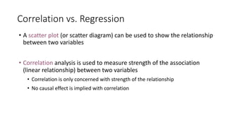
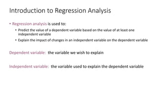
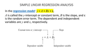
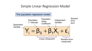
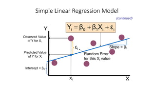
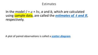
probability distribution term 1 IMI New Delhi.pdf

Business Statistics
PGDM (2023-24)
Term-II (Oct-Jan, 2023-24)
Ruchika Lochab
Assistant Professor, Operations
IMI, Delhi

Correlation and regression analysis
• Estimation using regression line
• Standard errors of estimate
• Correlation Analysis
• Coefficient of determination
• Coefficient of correlation

Correlation vs. Regression
• A scatter plot (or scatter diagram) can be used to show the relationship
between two variables
• Correlation analysis is used to measure strength of the association
(linear relationship) between two variables
• Correlation is only concerned with strength of the relationship
• No causal effect is implied with correlation

Introduction to Regression Analysis
• Regression analysis is used to:
• Predict the value of a dependent variable based on the value of at least one
independent variable
• Explain the impact of changes in an independent variable on the dependent variable
Dependent variable: the variable we wish to explain
Independent variable: the variable used to explain the dependent variable

• Regression and correlation analysis tell us how to determine both
the nature and the strength of a relationship between two
variables.
• Regression and correlation analysis are based on the relationship or
association between two or more variables.
• The known variable is called independent, and the unknown
variable we are trying to predict is the dependent variable.

Correlation Analysis
• Correlation analysis is a tool to describe the degree to which one variable is
linearly related to other.
• There are two measures for describing the correlation between two
variables—coefficient of determination and coefficient of correlation.
• The coefficient of determination is the primary way with which we can
measure the extent or strength of the association that exists between two
variables.
• Correlation value between -1 and 1 indicating the strength of the association
of the observed data for the two variables.

Simple Regression
A regression model is a mathematical equation that describes the
relationship between two or more variables.
A simple regression model includes only two variables:
one independent and one dependent.
The dependent variable is the one being explained, and the independent
variable is the one used to explain the variation in the dependent variable.

Linear Regression
A (simple) regression model that gives a straight-line relationship
between two variables is called a linear regression model.

SIMPLE LINEAR REGRESSION ANALYSIS
In the regression model y = A + Bx + ε,
A is called the y-intercept or constant term, B is the slope, and ε
is the random error term. The dependent and independent
variables are y and x, respectively.

i
i
1
0
i ε
X
β
β
Y +
+
=
Linear component
Simple Linear Regression Model
The population regression model:
Population
Y intercept
Population
Slope
Coefficient
Random
Error
term
Dependent
Variable
Independent
Variable
Random Error
component

(continued)
Random Error
for this Xi value
Y
X
Observed Value
of Y for Xi
Predicted Value
of Y for Xi
i
i
1
0
i ε
X
β
β
Y +
+
=
Xi
Slope = β1
Intercept = β0
εi

Estimates
In the model ŷ = a + bx, a and b, which are calculated
using sample data, are called the estimates of A and B,
respectively.
A plot of paired observations is called a scatter diagram.

i
1
0
i X
b
b
Ŷ +
=
The simple linear regression equation provides an estimate of the
population regression line
Simple Linear Regression Equation
Estimate of
the regression
intercept
Estimate of the
regression slope
Estimated
(or predicted)
Y value for
observation i
Value of X for
observation i
The individual random error terms ei have a mean of zero

Figure: The Estimation Process in Simple Linear Regression

Figure: Possible Regression Lines in Simple Linear Regression

• b0 is the estimated average value of Y when the value of
X is zero
• b1 is the estimated change in the average value of Y as a
result of a one-unit change in X
Interpretation of the Slope and the Intercept

Least Squares Method
• Least squares method: A procedure for using sample data to find
the estimated regression equation.
• Determine the values of 0 1
and .
b b
• Interpretation of 0 1
and :
b b
• The slope 1
b is the estimated change in the mean of the dependent
variable y that is associated with a one unit increase in the
independent variable x.
• The y-intercept 0
b is the estimated value of the dependent variable y
when the independent variable x is equal to 0.

• th
i residual: The error made using the regression model to estimate the
mean value of the dependent variable for the th
i observation.
• Denoted as ˆ .
i i i
e y y
= -
• Hence,
( )
2 2
1 1
ˆ
min min
n n
i i i
i i
y y e
= =
- =
å å
• We are finding the regression that minimizes the sum of squared
errors.

Error Sum of Squares (SSE)
The error sum of squares, denoted SSE, is
The values of a and b that give the minimum SSE are called the least
square estimates of A and B, and the regression line obtained with these
estimates is called the least squares line.
2 2
ˆ
SSE ( )
e y y
= = -
å å

The Least Squares Line
For the least squares regression line ŷ = a + bx,
SS
and
SS
xy
xx
b a y bx
= = -
where
and SS stands for “sum of squares.” The least squares
regression line ŷ = a + bx is also called the regression of y on
x.
( )( ) ( )
2
2
SS and SS
xy xx
x y x
xy x
n n
= - = -
å å å
å å

Example
Draw scatter plot, find the least squares regression line for the data on incomes
and food expenditure on the seven households given in the Table on next page.
Use income as an independent variable and food expenditure as a dependent
variable.
Table: Incomes (in
hundreds of
dollars) and Food
Expenditures of
Seven
Households

Solution 386 108
/ 386/7 55.1429
/ 108/7 15.4286
x y
x x n
y y n
= =
= = =
= = =
å å
å
å
( )( )
( )
2
2
2
(386)(108)
SS 6403 447.5714
7
(386)
SS 23,058 1772.8571
7
xy
xx
x y
xy
n
x
x
n
= - = - =
= - = - =
å å
å
å
å

Solution cntd.:
447.5714
.2525
1772.8571
15.4286 (.2525)(55.1429) 1.5050
xy
xx
SS
b
SS
a y bx
= = =
= - = - =
Thus, our estimated regression model is
ŷ = 1.5050 + .2525 x

Figure: Regression Line and random errors (General)

Interpretation of a
• Consider a household with zero income. Using the estimated
regression line obtained in Example,
ŷ = 1.5050 + .2525(0) = $1.5050 hundred.
• Thus, we can state that a household with no income is expected
to spend $150.50 per month on food.
• The regression line is valid only for the values of x between 33
and 83.

Interpretation of b
• The value of b in the regression model gives the
change in y (dependent variable) due to a change of
one unit in x (independent variable).
• We can state that, on average, a $100 (or $1) increase
in income of a household will increase the food
expenditure by $25.25 (or $.2525).

Calculate SSE for this example!!

Example: Least Squares Method
Table: Miles Traveled and
Travel Time for 10
Trucking Company Driving
Assignments
Driving Assignment i x = Miles Traveled
y = Travel Time
(hours)
1 100 9.3
2 50 4.8
3 50 8.9
4 100 6.5
5 50 4.2
6 80 6.2
7 75 7.4
8 65 6.0
9 90 7.6
10 90 6.1

Figure: Scatter
Chart of Miles
Traveled and Travel
Time for Sample of
10 Trucking
Company Driving
Assignments

Least Squares Estimates of the Regression Parameters:
• For the Trucking Company data in Table:
• Estimated slope of 1 0.0678.
b =
• y-intercept of 0 1.2739.
b =
• The estimated simple linear regression model:
1
ˆ 1.2739 0.0678
y x
= +

• Interpretation of 1:
b If the length of a driving assignment were 1 unit
(1 mile) longer, the mean travel time for that driving assignment
would be 0.0678 units (0.0678 hours, or approximately 4 minutes)
longer.
• Interpretation of 0:
b If the driving distance for a driving assignment
was 0 units (0 miles), the mean travel time would be 1.2739 units
(1.2739 hours, or approximately 76 minutes).

• Trucking Company example: Use the estimated model and the known
values for miles traveled for a driving assignment (x) to estimate mean
travel time in hours.
• For example, the first driving assignment in the Table has a value for miles
traveled of 100.
x =
• The mean travel time in hours for this driving assignment is estimated to be:
( )
1
ˆ 1.2739 0.0678 100 8.0539
y = + =
• The resulting residual of the estimate is:
1 1 1
ˆ 9.3 8.0539 1.2461
e y y
= - = - =

Table: Predicted Travel Time and Residuals for Butler Trucking Company
Driving Assignments

Figure: Scatter Chart of
Miles Traveled and Travel
Time for Trucking Company
Driving Assignments with
Regression Line
Superimposed

Figure: Scatter
Chart and
Estimated
Regression Line
for Trucking
Company

Least Squares Method (alternate formula)
Slope Equation
( )( )
( )
1
1
2
1
n
i i
i
n
i
i
x x y y
b
x x
=
=
- -
=
-
å
å
y-Intercept Equation
0 1
b y b x
= -
value of the independent variable for the th observation.
value of the dependent variable for the th observation.
mean value for the independent variable.
mean value for the dependent var
i
i
x i
y i
x
y
=
=
=
= iable.
total number of observations.
n =

STANDARD DEVIATION OF ERRORS AND COEFFICIENT OF DETERMINATION
Degrees of Freedom for a Simple Linear Regression
Model
The degrees of freedom for a simple linear regression
model are
df = n – 2

STANDARD DEVIATION OF ERRORS AND COEFFICIENT OF DETERMINATION
The standard deviation of errors is calculated as
where
2
yy xy
e
SS bSS
s
n
-
=
-
2
2
( )
yy
y
SS y
n
= -
å
å

Example
Compute the standard deviation of errors se for the data on monthly incomes and food expenditures of
the seven households given in Table.

Solution
( )
2
2
2 (108)
1792 125.7143
7
125.7143 .2525(447.5714)
1.5939
2 7 2
yy
yy xy
e
y
SS y
n
SS bSS
s
n
= - = - =
- -
= =
- -
å
å

Total Sum of Squares (SST)
The total sum of squares, denoted by SST, is calculated
as
Note that this is the same formula that we used to
calculate SSyy.
( )
2
2
y
SST y
n
= -
å
å

Figure: Errors of prediction when regression model is used.

Standard Error of Estimate
• The standard deviation of the variation of
observations around the regression line is estimated
by
2
n
)
Ŷ
Y
(
2
n
SSE
S
n
1
i
2
i
i
YX
-
-
=
-
=
å
=
Where
SSE = error sum of squares
n = sample size

Comparing Standard Errors
Y
Y
X X
YX
s
small YX
s
large
SYX is a measure of the variation of observed
Y values from the regression line
The magnitude of SYX should always be judged relative to the
size of the Y values in the sample data

Assumptions of Regression
• Normality of Error
• Error values (ε) are normally distributed for any given
value of X
• Homoscedasticity
• The probability distribution of the errors has constant
variance
• Independence of Errors
• Error values are statistically independent

Coefficient of Determination
The coefficient of determination, denoted by r2, represents the
proportion of SST that is explained by the use of the regression model.
The computational formula for r2 is
and 0 ≤ r2 ≤ 1
2 xy
yy
b SS
r
SS
=

Goodness of Fit of estimated model
YY X Y X
r2 = 0
r2 between 0 to 1
r2 represent the overlapping portion above.
r2 lies between 0 and 1. The higher the r2, the better the
estimated model.
Y Y= X
Y X
r2 = 1
r2 close to 1

Measures of Variation
• Total variation is made up of two parts:
SSE
SSR
SST +
=
Total Sum of
Squares
Regression Sum
of Squares
Error Sum of
Squares
å -
= 2
i )
Y
Y
(
SST å -
= 2
i
i )
Ŷ
Y
(
SSE
å -
= 2
i )
Y
Ŷ
(
SSR
where:
= Average value of the dependent variable
Yi = Observed values of the dependent variable
i = Predicted value of Y for the given Xi value
Ŷ
Y

• SST = total sum of squares
• Measures the variation of the Yi values around their mean Y
• SSR = regression sum of squares
• Explained variation attributable to the relationship between X and Y
• SSE = error sum of squares
• Variation attributable to factors other than the relationship between
X and Y
(continued)
Measures of Variation

• The coefficient of determination is the portion of
the total variation in the dependent variable that is
explained by variation in the independent variable
• The coefficient of determination is also called r-
squared and is denoted as r2
Coefficient of Determination, r2
1
r
0 2
£
£
note:
squares
of
sum
total
squares
of
sum
regression
SST
SSR
r2
=
=

r2 = 1
Examples of Approximate r2 Values
Y
X
Y
X
r2 = 1
r2 = 1
Perfect linear relationship
between X and Y:
100% of the variation in Y is
explained by variation in X

Examples of Approximate r2 Values
Y
X
Y
X
0 < r2 < 1
Weaker linear relationships
between X and Y:
Some but not all of the
variation in Y is explained
by variation in X

Examples of Approximate
r2 Values
r2 = 0
No linear relationship
between X and Y:
The value of Y does not
depend on X. (None of the
variation in Y is explained
by variation in X)
Y
X
r2 = 0

Example
For the data on monthly incomes and food expenditures of seven households, calculate the coefficient of
determination.
Solution:
• From earlier calculations
• b = .2525, 𝑺𝑺𝒙𝒚= 447.5714, 𝑺𝑺𝒚𝒚 = 125.7143
2 (.2525)(447.5714)
.90
125.7143
xy
yy
b SS
r
SS
= = =

Linear Correlation Coefficient
Value of the Correlation Coefficient
The value of the correlation coefficient always lies in the
range of –1 to 1; that is,
-1 ≤ ρ ≤ 1 and -1 ≤ r ≤ 1

Figure: Linear correlation between two variables.
(a) Perfect positive linear
correlation, r = 1
(b) Perfect negative linear
correlation, r = -1
(c) No linear
correlation, , r ≈ 0

Figure: Linear correlation between variables.

Linear Correlation Coefficient
The simple linear correlation coefficient, denoted by r,
measures the strength of the linear relationship between two
variables for a sample and is calculated as
xy
xx yy
SS
r
SS SS
=

Example Calculate the correlation coefficient for the example on incomes and food
expenditures of seven households.
447.5714
.95
(1772.8571)(125.7143)
xy
xx yy
SS
r
SS SS
=
= =
Solution:

INFERENCES ABOUT B (about Population Parameters)
• Sampling Distribution of b
• Estimation of B
• Hypothesis Testing About B

Sampling Distribution of b
Mean, Standard Deviation, and Sampling Distribution of b
Because of the assumption of normally distributed random errors, the sampling
distribution of b is normal. The mean and standard deviation of b, denoted by
and , respectively, are
and
b b
xx
B
SS
s
µ s Î
= =
b
µ
b
s

Estimation of B
Confidence Interval for B
The (1 – α)100% confidence interval for B is given by
where
and the value of t is obtained from the t distribution table for α α /2 area in the
right tail of the t distribution and n-2 degrees of freedom.
b
b ts
±
e
b
xx
s
s
SS
=

Example
Construct a 95% confidence interval for B for the data on incomes and food expenditures of
seven households given in Table.
Solution:
1.5939
.0379
1772.8571
2 7 2 5
/2 (1 .95)/2 .025
2.571
.2525 2.571(.0379)
.2525 .0974 .155 to .350
e
b
xx
b
s
s
SS
df n
t
b ts
a
= = =
= - = - =
= - =
=
± = ±
= ± =

Hypothesis Testing About B
Test Statistic for b
The value of the test statistic t for b is calculated as
The value of B is substituted from the null hypothesis.
b
b B
t
s
-
=

Example
Test at the 2% significance level whether the slope of the regression line for the example on incomes
and food expenditures of seven households is positive.
Solution:
• Step 1:
H0: B = 0 (The slope is zero)
H1: B > 0 (The slope is positive)
• Step 2:
is not known
Hence, we will use the t distribution to make the test
about B.
Î
s

Solution cntd.
• Step 3:
α = .02
Area in the right tail = α = .02
df = n – 2 = 7 – 2 = 5
The critical value of t is 3.365.

Solution cntd
.2525 0
6.662
.0379
b
b B
t
s
- -
= = =
From H0
q Step 4:

Solution cntd
• Step 5:
The value of the test statistic t = 6.662
• It is greater than the critical value of t = 3.365
• It falls in the rejection region
Hence, we reject the null hypothesis
We conclude that x (income) determines y (food
expenditure) positively.

Hypothesis Testing About the Linear Correlation Coefficient
Test Statistic for r
If both variables are normally distributed and the null hypothesis is
H0: ρ = 0,
then the value of the test statistic t is calculated as
Here n – 2 are the degrees of freedom.
2
2
1
n
t r
r
-
=
-

Example
Using the 1% level of significance and the data from Example, test whether the linear correlation coefficient
between incomes and food expenditures is positive. Assume that the populations of both variables are
normally distributed.
Solution:
• Step 1:
H0: ρ = 0 (The linear correlation coefficient is zero)
H1: ρ > 0 (The linear correlation coefficient is positive)
• Step 2:
The population distributions for both variables are normally distributed. Hence, we can use the
t distribution to perform this test about the linear correlation coefficient.

• Step 3:
Area in the right tail = .01
df = n – 2 = 7 – 2 = 5
The critical value of t = 3.365

q Step 4:
𝑡 = 𝒓
𝒏 − 𝟐
𝟏 − 𝒓𝟐
=. 𝟗𝟒𝟖𝟏
𝟕#𝟐
𝟏#(.𝟗𝟒𝟖𝟏)𝟐=6.667

• Step 5:
The value of the test statistic t = 6.667
• It is greater than the critical value of t=3.365
Hence, we reject the null hypothesis.
We conclude that there is a positive relationship
between incomes and food expenditures.

REGRESSION ANALYSIS: A COMPLETE Example
A random sample of eight drivers selected from a small city insured with a company and having similar
minimum required auto insurance policies was selected. The following table lists their driving experiences (in
years) and monthly auto insurance premiums (in dollars).

(a) Does the insurance premium depend on the driving experience or does the driving
experience depend on the insurance premium? Do you expect a positive or a
negative relationship between these two variables?
(b) Compute SSxx, SSyy, and SSxy.
(c) Find the least squares regression line by choosing appropriate dependent and
independent variables based on your answer in part a.
(d) Interpret the meaning of the values of a and b calculated in part c.
(e) Plot the scatter diagram and the regression line.
(f) Calculate r and r2 and explain what they mean.
(g) Predict the monthly auto insurance for a driver with 10 years of driving experience.
(h) Compute the standard deviation of errors.
(i) Construct a 90% confidence interval for B.
(j) Test at the 5% significance level whether B is negative.
(k) Using α = .05, test whether ρ is different from zero.

Solution
(a) Based on theory and intuition, we expect the insurance premium to depend on driving experience.
• The insurance premium is a dependent variable
• The driving experience is an independent variable

Solution
(b)
/ 90/8 11.25
/ 474/8 59.25
x x n
y y n
= = =
= = =
å
å
2 2
2
2 2
2
( )( ) (90)(474)
4739 593.5000
8
( ) (90)
1396 383.5000
8
( ) (474)
29,642 1557.5000
8
xy
xx
yy
x y
SS xy
n
x
SS x
n
y
SS y
n
= - = - = -
= - = - =
= - = - =
å å
å
å
å
å
å

Solution (c)
593.5000
1.5476
383.5000
59.25 ( 1.5476)(11.25) 76.6605
xy
xx
SS
b
SS
a y bx
-
= = = -
= - = - - =
ŷ = 𝟕𝟔. 𝟔𝟔𝟎𝟓 − 𝟏. 𝟓𝟒𝟕𝟔𝒙

Solution (d) and (e)
The value of a = 76.6605 gives the value of ŷ for x = 0; that is, it gives the monthly auto
insurance premium for a driver with no driving experience.
The value of b = -1.5476 indicates that, on average, for every extra year of driving
experience, the monthly auto insurance premium decreases by $1.55.
(e) The regression
line slopes
downward from
left to right.

Solution (f)
2
593.5000
.77
(383.5000)(1557.5000)
( 1.5476)( 593.5000)
.59
1557.5000
xy
xx yy
xy
yy
SS
r
SS SS
bSS
r
SS
-
= = = -
- -
= = =
The value of r = -0.77 indicates that the driving experience and the monthly auto insurance
premium are negatively related.
The (linear) relationship is strong but not very strong.
The value of r² = 0.59 states that 59% of the total variation in insurance premiums is
explained by years of driving experience and 41% is not.

Solution (g)
Using the estimated regression line, we find the predicted value of y for x = 10 is
ŷ = 76.6605 – 1.5476(10) = $61.18
Thus, we expect the monthly auto insurance premium of a driver with 10 years of driving experience to be
$61.18.
(h)
2
1557.5000 ( 1.5476)( 593.5000)
8 2
10.3199
yy xy
e
SS bSS
s
n
-
=
-
- - -
=
-
=

Solution (i)
10.3199
.5270
383.5000
/2 .5 (.90/2) .05
2 8 2 6
1.943
1.5476 1.943(.5270)
1.5476 1.0240 2.57 to .52
e
b
xx
b
s
s
SS
df n
t
b ts
a
= = =
= - =
= - = - =
=
± = - ±
= - ± = - -

Solution (j)
• Step 1:
H0: B = 0 (B is not negative)
H1: B < 0 (B is negative)
• Step 2: Because the standard deviation of the error is not known, we use the t distribution to
make the hypothesis test
• Step 3:
Area in the left tail = α = .05
df = n – 2 = 8 – 2 = 6
The critical value of t is -1.943

1.5476 0
2.937
.5270
b
b B
t
s
- - -
= = =-
From H0
q Step 4:

• Step 5:
The value of the test statistic t = -2.937
Hence, we reject the null hypothesis and conclude that B is
negative.
The monthly auto insurance premium decreases with an
increase in years of driving experience.

Solution (k)
• Step 1:
H0: ρ = 0 (The linear correlation coefficient is zero)
H1: ρ ≠ 0 (The linear correlation coefficient is different from zero)
• Step 2: Assuming that variables x and y are normally distributed, we will use the t distribution to
perform this test about the linear correlation coefficient.
• Step 3:
Area in each tail = .05/2 = .025
df = n – 2 = 8 – 2 = 6
The critical values of t are -2.447 and 2.447

q Step 4:
𝒕 = 𝒓
𝒏 − 𝟐
𝟏 − 𝒓𝟐
= −. 𝟕𝟔𝟕𝟗
𝟖#𝟐
𝟏#(#.𝟕𝟕)𝟐= -2.936

• Step 5:
The value of the test statistic t = -2.936
Hence, we reject the null hypothesis
We conclude that the linear correlation coefficient
between driving experience and auto insurance premium is
different from zero.

probability distribution term 1 IMI New Delhi.pdf

More Related Content

Similar to probability distribution term 1 IMI New Delhi.pdf

Recently uploaded

probability distribution term 1 IMI New Delhi.pdf