Data Structures Introduction

1. Elementary Data Organization
• Data are simply values or sets of values.
• Collection of data are frequently organized into a
hierarchy of fields, records and files.

2. 2
Data Structures
 Data Structures
The logical or mathematical model of a particular organization of data is called a data
structure.
 Types of Data Structure
1. Linear Data Structure
Example: Arrays, Linked Lists, Stacks, Queues
2. Nonlinear Data Structure
Example: Trees, Graphs
A
B C
D E F
A B C D E F
Figure: Linear and nonlinear structures
Array Tree

3. 3
Choice of Data Structures
The choice of data structures depends on two considerations:
1. It must be rich enough in structure to mirror the actual relationships of data in the
real world.
2. The structure should be simple enough that one can effectively process data when
necessary.
10
20
30
40
50
60
70
80
10
20 30
40 50 60 70
Figure 2: Array with 8 items Figure 3: Tree with 8 nodes

4. 4
Data Structure Operations
1. Traversing: Accessing each record exactly once so that certain items in the
record may be processed.
2. Searching: Finding the location of the record with a given key value.
3. Inserting: Adding a new record to the structure.
4. Deleting: Removing a record from the structure.
5. Sorting: Arranging the records in some logical order.
6. Merging: Combining the records in two different sorted files into a single
sorted file.
The choice of data structure depends on many things,
including the type of the data and the frequency with which
various operations are performed on data.

5. 5
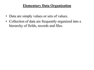
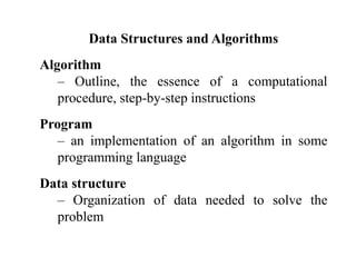
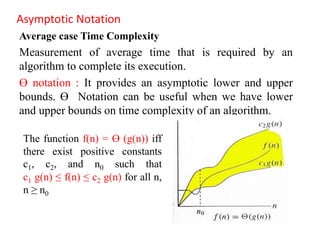
Algorithms
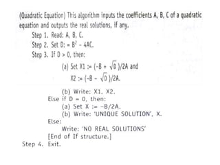
An algorithm is a well-defined set of instructions used to solve a particular
problem.
Example:
Write an algorithm for finding the location of the largest element of an array Data.
Largest-Item (Data, N, Loc)
1. set k:=1, Loc:=1 and Max:=Data[1]
2. while k<=N repeat steps 3, 4
3. If Max < Data[k] then Set Loc:=k and Max:=Data[k]
4. Set k:=k+1
5. write: Max and Loc
6. exit

6. Data Structures and Algorithms
Algorithm
– Outline, the essence of a computational
procedure, step-by-step instructions
Program
– an implementation of an algorithm in some
programming language
Data structure
– Organization of data needed to solve the
problem

7. 7
Complexity of Algorithms
• The complexity of an algorithm is the function f(n) which
gives the running time and/or storage space requirement of
the algorithm in terms of the size n of the input data.
• Two types of complexities
1. Time Complexity – running time of an algorithm
2. Space Complexity – space required by an algorithm
The choice of data structure involves a time-space trade-off:
by increasing the amount of space for storing the data one
may be able to reduce the time needed for processing of data
or vice versa.

8. Time Complexity
‐ The amount of time needed by a program to complete its
execution
‐ Measurement of time is done in terms of number of
instructions executed by the program
‐ Depends on the size of the program and type of the
algorithm used
Space Complexity
‐ The amount of memory needed by a program to complete
its execution
‐ Total memory space needed by the program is divided into
two parts
‐ Fixed size memory
‐ Variable size memory

9. Performance Analysis
 Space Complexity
 Time Complexity
Space Complexity
The amount of memory required by an
algorithm for its completion
Fixed part - independent of input & output
Variable part - dependent on particular problem
S(p) = c + Sp
c is constant, Sp is instance characteristics

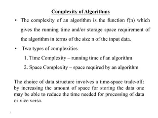
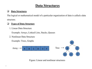
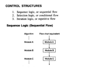
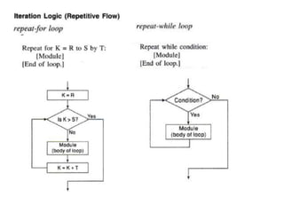
10. Time Complexity
The amount of computer time required by an
algorithm for its completion
Algorithm sum (a,n)
{
s := 0;
for i:= 1 to n do
s := s+a[i];
return s; Space : n+3
} Time : 2n+3

11. Complexity of an algorithm
 It is a measure that indicates the resource
requirement in terms of n to complete a
task
 Resources can be memory, time etc.
 Space is measured in terms of amount of
memory space required
 Time is measured in terms of no. of
computations required. We do not find
exact computations, but we find only
proportionality expressions in terms of n.

12.  The performance of an algorithm depends
on the input data
Best case complexity - Ω (omega)
Average case complexity - Ө (theta)
Worst case complexity - О (big oh)

13. Asymptotic Notation
Best case Time Complexity
Measurement of minimum time that is required by an
algorithm to complete its execution.
Ω notation : It provides an asymptotic lower bound. Ω
Notation can be useful when we have lower bound on time
complexity of an algorithm.
The function f(n) = Ω (g(n)) iff
there exist positive constants
c and n0 such that f(n) ≥ c * g(n)
for all n, n ≥ n0

14. Asymptotic Notation
Worst case Time Complexity
Measurement of maximum time that is required by an
algorithm to complete its execution.
O notation : It provides an asymptotic upper bound. O
Notation can be useful when we have upper bound on time
complexity of an algorithm.
The function f(n) = O (g(n)) iff
there exist positive constants
c and n0 such that f(n) ≤ c * g(n)
for all n, n ≥ n0

15. Asymptotic Notation
Average case Time Complexity
Measurement of average time that is required by an
algorithm to complete its execution.
Ө notation : It provides an asymptotic lower and upper
bounds. Ө Notation can be useful when we have lower
and upper bounds on time complexity of an algorithm.
The function f(n) = Ө (g(n)) iff
there exist positive constants
c1, c2, and n0 such that
c1 g(n) ≤ f(n) ≤ c2 g(n) for all n,
n ≥ n0

16. 16
Example:
(a) f(n) = 3n+2
Here f(n) <= 5n for n>=1
So, f(n) = O(n).
(b) f(n) = 3n2-2
Here f(n) < 3n2 for n>=1
So, f(n) = O(n2).

17. Function Name
c Constant
logn Logarithmic
log2n Log-squared
n Linear
nlogn nlogn
n2 Quadratic
n3 Cubic
2n Exponential
17
Typical Growth Rates

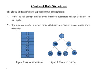
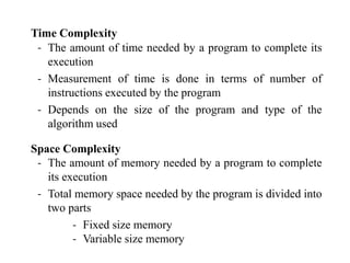
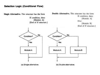
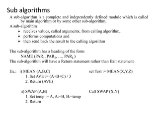
18. Comments:
‐ Each step may contain a comment in brackets [ ], indicates the
main purpose of the step.
‐ Usually appear at the beginning or the end of the step.
Variable names :
‐ Variable names will use capital letters. Ex.: MAX, DATA, SUM
‐ Single-letter names of variables used as counters or subscripts
will use capital letters. Ex. : I, K, N etc.
Assignment Statement :
‐ It uses the colon-equal notation (:=). Ex. : C := A + B
Input and output :
‐ Data may be input and assigned to variables using Read
statement
Read : Variable names
‐ Data in variables and messages (placed in quotation marks) may
be output by using Write or Print statement
Write : Messages and / or variable names

24. Sub algorithms
A sub-algorithm is a complete and independently defined module which is called
by main algorithm or by some other sub-algorithm.
A sub-algorithm
 receives values, called arguments, from calling algorithm,
 performs computations and
 then send back the result to the calling algorithm
The sub-algorithm has a heading of the form
NAME (PAR1, PAR2, …, PARk )
The sub-algorithm will have a Return statement rather than Exit statement
Ex.: i) MEAN (A,B,C) set Test := MEAN(X,Y,Z)
1. Set AVE := (A+B+C) / 3
2. Return (AVE)
ii) SWAP (A,B) Call SWAP (X,Y)
1. Set temp := A, A:=B, B:=temp
2. Return

25. Sub algorithms
 Function sub-algorithm returns only a single value to the
calling function
 Procedure sub-algorithm may send back more than one
value
Local and Global variables
Each module contains its own list of variables, called local variables, which
can be accessed only by the given module
Variables that can be accessed by all the program modules are called global
variables
In two ways modules can communicate
Directly : by way of well-defined parameters
Indirectly : by way of non-local and global variables

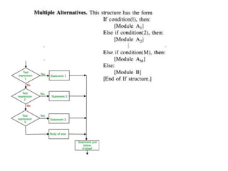
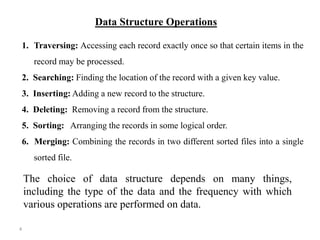
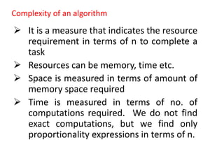
26. Procedure to find the locations of largest and second largest elements of array
FIND (DATA, N, LOC1, LOC2)
1) Set FIRST := DATA[1], SECOND := DATA [2]
LOC1 := 1, LOC2 := 2
2) If FIRST < SECOND, then
a) Interchange FIRST and SECOND
b) set LOC1 := 2, LOC2 := 1
3) Repeat for K = 3 to N
If FIRST < DATA[K], then
a) set SECOND := FIRST and FIRST := DATA[K]
b) set LOC2 := LOC1 and LOC1 := K
else if SECOND < DATA[K], then
set SECOND := DATA[K] and LOC2 := K
4) Return

27. Procedure to find prime numbers less than a given number m, using Sieve method
Algorithm:
1. Repeat for K = 1 to N :
Set A[K] := K
2. Repeat for K = 2 to √N:
Call CROSSOUT (A,N,K)
3. Repeat for K = 2 to N:
If A[K] ≠ 1, then : Write : A[K]
4. Exit
CROSSOUT(A,N,K)
1. If A[K] = 1, then : Return.
2. Repeat for L = 2K to N by K:
Set A[L] := 1.
3. Return