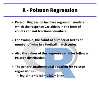
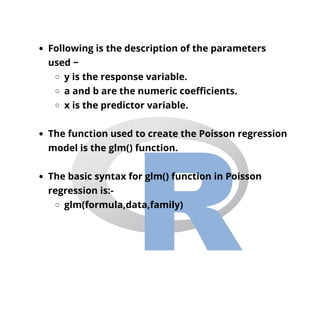
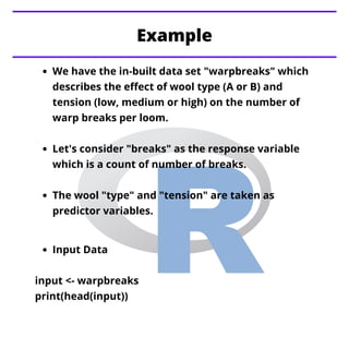
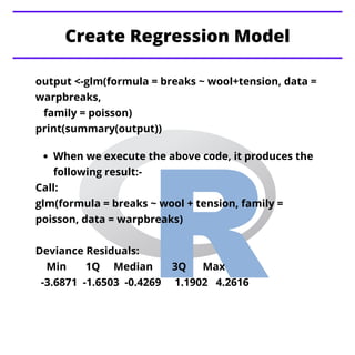
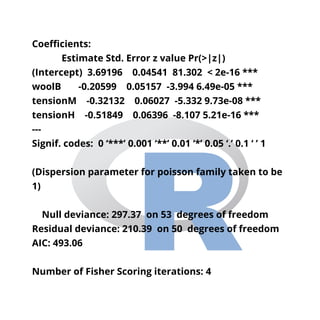
This document discusses Poisson regression in R. Poisson regression is a type of regression where the response variable is counts, like number of births or wins. The document shows how to create a Poisson regression model in R using the glm() function, specifying the Poisson family. It uses the built-in warpbreaks data to predict the number of warp breaks based on wool type and tension level, and the summary of the model shows that wool type B and higher tension levels have a significant impact on the number of breaks.

1. Swipe
R - Poisson Regression

2. Poisson Regression involves regression models in
which the response variable is in the form of
counts and not fractional numbers.
For example, the count of number of births or
number of wins in a football match series.
Also the values of the response variables follow a
Poisson distribution.
The general mathematical equation for Poisson
regression is:-
log(y) = a + b1x1 + b2x2 + bnxn
R - Poisson Regression

3. Following is the description of the parameters
used −
y is the response variable.
a and b are the numeric coefficients.
x is the predictor variable.
The function used to create the Poisson regression
model is the glm() function.
The basic syntax for glm() function in Poisson
regression is:-
glm(formula,data,family)

4. Following is the description of the parameters
used in above functions −
formula is the symbol presenting the
relationship between the variables.
data is the data set giving the values of these
variables.
family is R object to specify the details of the
model. It's value is 'Poisson' for Logistic
Regression.

5. Example
We have the in-built data set "warpbreaks" which
describes the effect of wool type (A or B) and
tension (low, medium or high) on the number of
warp breaks per loom.
Let's consider "breaks" as the response variable
which is a count of number of breaks.
The wool "type" and "tension" are taken as
predictor variables.
Input Data
input <- warpbreaks
print(head(input))

6. When we execute the above code, it produces the
following result:-
breaks wool tension
1 26 A L
2 30 A L
3 54 A L
4 25 A L
5 70 A L
6 52 A L

7. Create Regression Model
output <-glm(formula = breaks ~ wool+tension, data =
warpbreaks,
family = poisson)
print(summary(output))
When we execute the above code, it produces the
following result:-
Call:
glm(formula = breaks ~ wool + tension, family =
poisson, data = warpbreaks)
Deviance Residuals:
Min 1Q Median 3Q Max
-3.6871 -1.6503 -0.4269 1.1902 4.2616

8. Coefficients:
Estimate Std. Error z value Pr(>|z|)
(Intercept) 3.69196 0.04541 81.302 < 2e-16 ***
woolB -0.20599 0.05157 -3.994 6.49e-05 ***
tensionM -0.32132 0.06027 -5.332 9.73e-08 ***
tensionH -0.51849 0.06396 -8.107 5.21e-16 ***
---
Signif. codes: 0 ‘***’ 0.001 ‘**’ 0.01 ‘*’ 0.05 ‘.’ 0.1 ‘ ’ 1
(Dispersion parameter for poisson family taken to be
1)
Null deviance: 297.37 on 53 degrees of freedom
Residual deviance: 210.39 on 50 degrees of freedom
AIC: 493.06
Number of Fisher Scoring iterations: 4

9. In the summary we look for the p-value in the last
column to be less than 0.05 to consider an impact
of the predictor variable on the response variable.
As seen the wooltype B having tension type M and
H have impact on the count of breaks.

10. R - Time Series Analysis
R - Nonlinear Least Square
R - Decision Tree
Stay Tuned with
Topics for next Post