Download to read offline


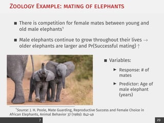


![Example: Poisson regression curve
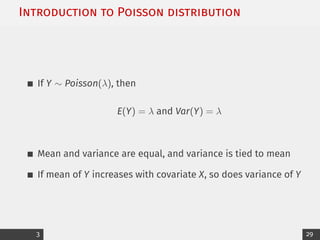
Add fitted curve to scatterplot:
1 coeffs <− coefficients (
elephant_poisson )
2 xvalues <− sort ( elephant$
Age )
3 means <− exp ( coeffs [ 1 ] +
coeffs [ 2 ] * xvalues )
4 lines ( xvalues , means , l t y
=2 , col = " red " )
30 35 40 45 50
0
2
4
6
8
Age
Number
of
Mates
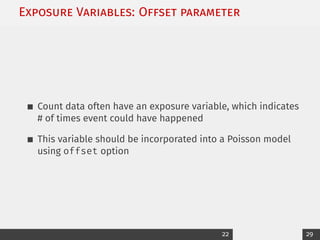
Poisson regression is a nonlinear model for E[Y]
10 29](https://image.slidesharecdn.com/9poissonprintable-230323163810-a0f27393/85/9_Poisson_printable-pdf-11-320.jpg)


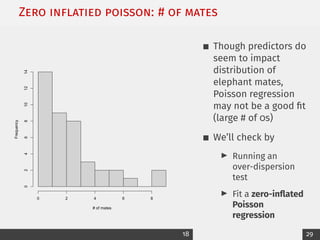


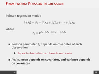
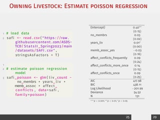
![What predicts owning more livestock?
Outcome: Livestock count [1-5]
Predictors:
I # of years lived in village
I # of people who live in household
I Whether they’re apart of a farmer cooperative
I Conflict with other farmers
24 29](https://image.slidesharecdn.com/9poissonprintable-230323163810-a0f27393/85/9_Poisson_printable-pdf-25-320.jpg)


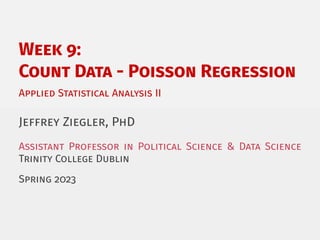
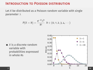
This document summarizes a lecture on Poisson regression for count data. It begins with an introduction to the Poisson distribution and its properties. It then discusses the framework of Poisson regression, using a log link function to model the Poisson parameter as a function of covariates. An example using elephant mating data is analyzed using Poisson regression. Model fitting, interpretation of coefficients, and obtaining fitted values are demonstrated. Finally, issues like overdispersion and zero-inflated models are discussed.


