Downloaded 12 times


![Quiz: What’s the Name of This Flower?
Oleg Yunakov [CC BY-SA 3.0 (https://creativecommons.org/licenses/by-sa/3.0)], from Wikimedia
Commons.
4 / 45](https://image.slidesharecdn.com/rdm-slides-data-exploration-visualisation-190703041148/85/RDataMining-slides-data-exploration-visualisation-4-320.jpg)
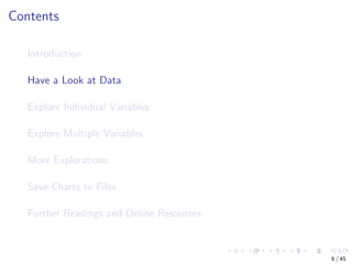
![The Iris Dataset
The iris dataset [Frank and Asuncion, 2010] consists of 50
samples from each of three classes of iris flowers. There are five
attributes in the dataset:
sepal length in cm,
sepal width in cm,
petal length in cm,
petal width in cm, and
class: Iris Setosa, Iris Versicolour, and Iris Virginica.
Detailed desription of the dataset can be found at the UCI
Machine Learning Repository †.
†
https://archive.ics.uci.edu/ml/datasets/Iris
5 / 45](https://image.slidesharecdn.com/rdm-slides-data-exploration-visualisation-190703041148/85/RDataMining-slides-data-exploration-visualisation-5-320.jpg)
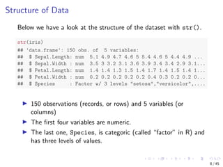
![Size and Variables Names of Data
# number of rows
nrow(iris)
## [1] 150
# number of columns
ncol(iris)
## [1] 5
# dimensionality
dim(iris)
## [1] 150 5
# column names
names(iris)
## [1] "Sepal.Length" "Sepal.Width" "Petal.Length" "Petal.Wid...
## [5] "Species"
7 / 45](https://image.slidesharecdn.com/rdm-slides-data-exploration-visualisation-190703041148/85/RDataMining-slides-data-exploration-visualisation-7-320.jpg)
![Attributes of Data
attributes(iris)
## $names
## [1] "Sepal.Length" "Sepal.Width" "Petal.Length" "Petal.Wid...
## [5] "Species"
##
## $class
## [1] "data.frame"
##
## $row.names
## [1] 1 2 3 4 5 6 7 8 9 10 11 12 13 ...
## [16] 16 17 18 19 20 21 22 23 24 25 26 27 28 ...
## [31] 31 32 33 34 35 36 37 38 39 40 41 42 43 ...
## [46] 46 47 48 49 50 51 52 53 54 55 56 57 58 ...
## [61] 61 62 63 64 65 66 67 68 69 70 71 72 73 ...
## [76] 76 77 78 79 80 81 82 83 84 85 86 87 88 ...
## [91] 91 92 93 94 95 96 97 98 99 100 101 102 103 1...
## [106] 106 107 108 109 110 111 112 113 114 115 116 117 118 1...
## [121] 121 122 123 124 125 126 127 128 129 130 131 132 133 1...
## [136] 136 137 138 139 140 141 142 143 144 145 146 147 148 1...
9 / 45](https://image.slidesharecdn.com/rdm-slides-data-exploration-visualisation-190703041148/85/RDataMining-slides-data-exploration-visualisation-9-320.jpg)
![First/Last Rows of Data
iris[1:3, ]
## Sepal.Length Sepal.Width Petal.Length Petal.Width Species
## 1 5.1 3.5 1.4 0.2 setosa
## 2 4.9 3.0 1.4 0.2 setosa
## 3 4.7 3.2 1.3 0.2 setosa
head(iris, 3)
## Sepal.Length Sepal.Width Petal.Length Petal.Width Species
## 1 5.1 3.5 1.4 0.2 setosa
## 2 4.9 3.0 1.4 0.2 setosa
## 3 4.7 3.2 1.3 0.2 setosa
tail(iris, 3)
## Sepal.Length Sepal.Width Petal.Length Petal.Width Spe...
## 148 6.5 3.0 5.2 2.0 virgi...
## 149 6.2 3.4 5.4 2.3 virgi...
## 150 5.9 3.0 5.1 1.8 virgi...
10 / 45](https://image.slidesharecdn.com/rdm-slides-data-exploration-visualisation-190703041148/85/RDataMining-slides-data-exploration-visualisation-10-320.jpg)
![A Single Column
The first 10 values of Sepal.Length
iris[1:10, "Sepal.Length"]
## [1] 5.1 4.9 4.7 4.6 5.0 5.4 4.6 5.0 4.4 4.9
iris$Sepal.Length[1:10]
## [1] 5.1 4.9 4.7 4.6 5.0 5.4 4.6 5.0 4.4 4.9
11 / 45](https://image.slidesharecdn.com/rdm-slides-data-exploration-visualisation-190703041148/85/RDataMining-slides-data-exploration-visualisation-11-320.jpg)
![library(Hmisc)
# describe(iris) # check all columns
describe(iris[, c(1, 5)]) # check columns 1 and 5
## iris[, c(1, 5)]
##
## 2 Variables 150 Observations
## -----------------------------------------------------------...
## Sepal.Length
## n missing distinct Info Mean Gmd ...
## 150 0 35 0.998 5.843 0.9462 4....
## .10 .25 .50 .75 .90 .95
## 4.800 5.100 5.800 6.400 6.900 7.255
##
## lowest : 4.3 4.4 4.5 4.6 4.7, highest: 7.3 7.4 7.6 7.7 7.9
## -----------------------------------------------------------...
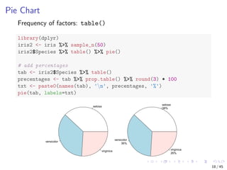
## Species
## n missing distinct
## 150 0 3
##
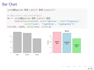
## Value setosa versicolor virginica
## Frequency 50 50 50
## Proportion 0.333 0.333 0.333
## -----------------------------------------------------------...
14 / 45](https://image.slidesharecdn.com/rdm-slides-data-exploration-visualisation-190703041148/85/RDataMining-slides-data-exploration-visualisation-14-320.jpg)
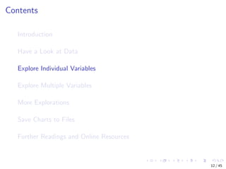
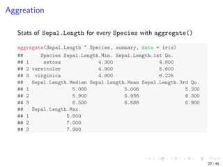
![Mean, Median, Range and Quartiles
Mean, median and range: mean(), median(), range()
Quartiles and percentiles: quantile()
range(iris$Sepal.Length)
## [1] 4.3 7.9
quantile(iris$Sepal.Length)
## 0% 25% 50% 75% 100%
## 4.3 5.1 5.8 6.4 7.9
quantile(iris$Sepal.Length, c(0.1, 0.3, 0.65))
## 10% 30% 65%
## 4.80 5.27 6.20
15 / 45](https://image.slidesharecdn.com/rdm-slides-data-exploration-visualisation-190703041148/85/RDataMining-slides-data-exploration-visualisation-15-320.jpg)
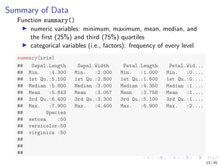
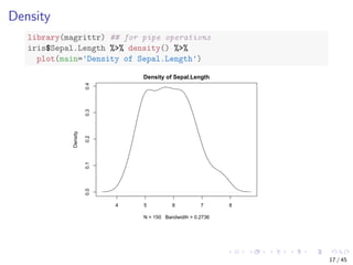
![Variance and Histogram
var(iris$Sepal.Length)
## [1] 0.6856935
hist(iris$Sepal.Length)
Histogram of iris$Sepal.Length
iris$Sepal.Length
Frequency
4 5 6 7 8
051015202530
16 / 45](https://image.slidesharecdn.com/rdm-slides-data-exploration-visualisation-190703041148/85/RDataMining-slides-data-exploration-visualisation-16-320.jpg)
![Correlation
Covariance and correlation: cov() and cor()
cov(iris$Sepal.Length, iris$Petal.Length)
## [1] 1.274315
cor(iris$Sepal.Length, iris$Petal.Length)
## [1] 0.8717538
cov(iris[, 1:4])
## Sepal.Length Sepal.Width Petal.Length Petal.Width
## Sepal.Length 0.6856935 -0.0424340 1.2743154 0.5162707
## Sepal.Width -0.0424340 0.1899794 -0.3296564 -0.1216394
## Petal.Length 1.2743154 -0.3296564 3.1162779 1.2956094
## Petal.Width 0.5162707 -0.1216394 1.2956094 0.5810063
# cor(iris[,1:4])
21 / 45](https://image.slidesharecdn.com/rdm-slides-data-exploration-visualisation-190703041148/85/RDataMining-slides-data-exploration-visualisation-21-320.jpg)
![Heat Map
Calculate the similarity between different flowers in the iris data
with dist() and then plot it with a heat map
dist.matrix <- as.matrix(dist(iris[, 1:4]))
heatmap(dist.matrix)
422314943394132463674831634154561921322425274417333749112247202631303510385411250284082918111910612313211813110811013613010312610114412114561999458658081826383936860709054107855667627291899796100955276665755598869987586797492641091371051251411461421401131041381171161491291331151351121111487853518777841501471241341271281397173120122114102143
422314943394132463674831634154561921322425274417333749112247202631303510385411250284082918111910612313211813110811013613010312610114412114561999458658081826383936860709054107855667627291899796100955276665755598869987586797492641091371051251411461421401131041381171161491291331151351121111487853518777841501471241341271281397173120122114102143
30 / 45](https://image.slidesharecdn.com/rdm-slides-data-exploration-visualisation-190703041148/85/RDataMining-slides-data-exploration-visualisation-30-320.jpg)
![Parallel Coordinates
Visualising multiple dimensions
library(MASS)
parcoord(iris[1:4], col = iris$Species)
Sepal.Length Sepal.Width Petal.Length Petal.Width
34 / 45](https://image.slidesharecdn.com/rdm-slides-data-exploration-visualisation-190703041148/85/RDataMining-slides-data-exploration-visualisation-34-320.jpg)
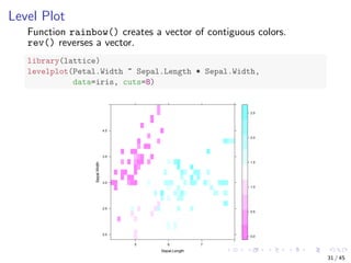
![Parallel Coordinates with Package lattice
library(lattice)
parallelplot(~iris[1:4] | Species, data = iris)
Sepal.Length
Sepal.Width
Petal.Length
Petal.Width
Min Max
setosa versicolor
Sepal.Length
Sepal.Width
Petal.Length
Petal.Width
virginica
35 / 45](https://image.slidesharecdn.com/rdm-slides-data-exploration-visualisation-190703041148/85/RDataMining-slides-data-exploration-visualisation-35-320.jpg)


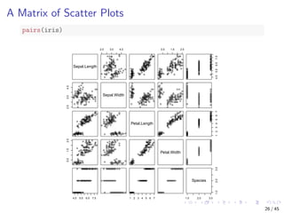
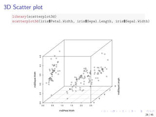
This document discusses exploring and visualizing data in R. It introduces the iris dataset and explores its structure and variables. Various summary statistics and charts are demonstrated, including histograms, density plots, scatter plots, boxplots and heat maps to explore individual and relationships between multiple variables. Multivariate exploration techniques like 3D scatter plots and pairwise plots are also covered. The document demonstrates how to save charts to files.


![[1062BPY12001] Data analysis with R / April 19](https://cdn.slidesharecdn.com/ss_thumbnails/dataanalyzer05control-180419065850-thumbnail.jpg?width=640&height=640&fit=bounds)